Analytic Planetary Transit Light Curves and Derivatives for Stars with Polynomial Limb Darkening

Abstract

We derive analytic, closed-form solutions for the light curve of a planet transiting a star with a limb darkening profile which is a polynomial function of the stellar elevation, up to arbitrary integer order. We provide improved analytic expressions for the uniform, linear, and quadratic limb-darkened cases, as well as novel expressions for higher order integer powers of limb darkening. The formulae are crafted to be numerically stable over the expected range of usage. We additionally present analytic formulae for the partial derivatives of instantaneous flux with respect to the radius ratio, impact parameter, and limb darkening coefficients. These expressions are rapid to evaluate, and compare quite favorably in speed and accuracy to existing transit light curve codes. We also use these expressions to numerically compute the first partial derivatives of exposure-time averaged transit light curves with respect to all model parameters. An additional application is modeling eclipsing binary or eclipsing multiple star systems in cases where the stars may be treated as spherically symmetric. We provide code which implements these formulae in C++, Python, IDL, and Julia, with tests and examples of usage.

1 Introduction

The precise measurement of the transits of an exoplanet offers a host of information about the planet’s properties (Charbonneau et al., 2007; Winn, 2008, 2010; Haswell, 2010). To start with, the times of transit give the planet’s orbital ephemeris. The depth of transit, corrected for stellar limb darkening, gives the planet’s radius relative to that of the star (Heller, 2019). The shape of the transit, especially the duration of ingress and egress relative to the full transit duration, yields the orbital impact parameter of the planet, which constrains the inclination of the orbit relative to the observer (Seager & Mallen-Ornelas, 2003). Beyond these basic properties, if the transit depth is seen to vary with wavelength, the presence of spectral features may be used to constrain the chemical composition of the planet’s atmosphere (Brown, 2001; Seager & Deming, 2010; Burrows, 2014; Crossfield, 2015; Madhusudhan, 2019). If the transit times are seen to vary, a dynamical model can constrain the masses of the planet companions, and vice versa (Agol et al., 2005; Holman, 2005). If the planet is seen in eclipse, its temperature, emission spectrum, and atmospheric circulation pattern can be constrained (Cowan & Fujii, 2017; Alonso, 2018). When combined with radial velocity measurements, the bulk density of a planet can be inferred, yielding constraints on its bulk composition (Udry et al., 2007).

And yet, all of these inferences are predicated on the precise computation of models of the planetary transit which may be used to infer the model parameters. Stars are non-uniform in brightness, with the general trend of growing dimmer towards the limb, and so limb darkening must be accounted for to accurately infer the planetary parameters (Csizmadia, 2018). Indeed, fast and accurate computation of limb-darkened transit light curve models has enabled the detection and characterization of thousands of transiting exoplanets (Mandel & Agol, 2002). The most important ingredient to these models has been a description of the limb darkening model which is flexible enough and accurate enough to describe the emission from a stellar photosphere. Linear and quadratic limb darkening laws were sufficient for lower-precision measurements; however, the measurement of transit light curves has steadily improved in precision. Higher order terms or non-linear laws have become necessary to describe higher precision measurements (Kopal, 1950; Claret, 2000; Giménez, 2006), which tend to involve more computational burden.

In addition to computing transit light curves, the derivatives of these light curves with respect to the model parameters are also beneficial for accurate characterization of exoplanets. The derivatives enable fast and stable optimization of the transit light curve parameters, which is critical for obtaining initial estimates for a Markov Chain Monte Carlo simulation (MCMC; e.g. Ford, 2005, 2006), for looking for multi-modal solutions, for initializing the multi-nest algorithm (Feroz & Hobson, 2008), or for computing the Fisher information matrix (Vallisneri, 2008). In some cases, MCMC can be slow to converge, and derivatives can accelerate convergence by adding an artificial momentum term to the log likelihood, and then allowing the sampler to follow contours of constant “energy.” This so-called “hybrid” or “Hamiltonian” MCMC approach holds great promise (Neal et al., 2011; Girolami & Calderhead, 2011; Betancourt, 2017), but its application has been hampered by the lack of models with derivatives, as derivatives are in general more difficult to compute.

Finally, the analytic computation of transit light curves with quadratic limb darkening has a precision which can be limited by numerical round-off error for parameters near some special cases. In particular, when the radius equals the impact-parameter, which corresponds to the edge of the planet crossing the center of the star, the computation of the elliptic integrals becomes unstable. At the second and third points of contact, when the radius of the planet plus the impact parameter equals the radius of the star, the elliptic integrals diverge logarithmically. In the limit that the impact parameter approaches zero, the equations can also diverge. All of these special cases are in principle encountered rarely, but in practice with thousand of planets with tens to thousands of transits each, along with hundreds to hundreds of thousands of light curves with time sub-sampled for each exposure, these rare cases can be encountered with some frequency.

Based on these considerations, the primary goals of the current paper are threefold:

1. To extend the analytic quadratic transit model to higher order limb darkening.

2. To compute the derivatives of the model analytically.

3. To stabilize the analytic light curve computation (and its derivatives) in all limits near special cases.

Secondary goals include modeling eclipsing binaries, for which the same considerations apply, and integrating the light curve model, and its derivatives, quickly and accurately over time to account for finite exposure times.

Some progress has been made already towards these goals. To describe this progress, we pause first to introduce some notation. Limb darkening models of spherical stars are parameterized with the cosine of the angle measured from the sub-stellar point, $\upmu=\cos{\theta}$, where $\theta$ is the polar angle on the photosphere, with $\theta=0$ at the center of the observed stellar disk, and $\theta=\pi/2$ at the limb. In a coordinate system in which the projected disk of the star lies in the $x-y$ plane, and the $z$ coordinate points towards the observer, then $\upmu=z$, where $x$, $y$, and $z$ are measured in units of the stellar radius. The variable $\upmu=z$ is then the elevation on the surface of the star, where the highest point is taken to be closest to the observer. In terms of $b=\sqrt{x^{2}+y^{2}}$, the normalized separation projected onto the sky, this parameter is given by $\upmu=\sqrt{1-b^{2}}$, where $0\leq b\leq 1$ within the stellar disk. We also introduce the radius ratio, $r$, which is the radius of the occultor divided by the radius of the source. In general, we will follow the notation introduced by Luger et al. (2019a) for the starry code package.

Uniform limb darkening scales as $I(\upmu)\propto\upmu^{0}$, first-order limb darkening as $I(\upmu)\propto\upmu^{1}$, and second-order limb darkening as $I(\upmu)\propto\upmu^{2}$; these are the three most commonly used terms that can be integrated analytically, which we describe in detail below in sections 3, 4, and 5. These are typically combined to yield the quadratic limb darkening law,

$$\frac{I(\upmu)}{I_{0}}=1-u_{1}(1-\upmu)-u_{2}(1-\upmu)^{2},$$ (1)

where $u_{1}$ and $u_{2}$ are the limb darkening parameters, and $I_{0}\equiv I(1)$ is a normalization constant, equal to the intensity at the center of the stellar disk. In this paper, we will show that higher order powers of $\upmu^{n}$ with integer $n$ can be integrated analytically for $n>2$ when expressed as recursion relations. Linear combinations of these laws can be constructed, with various parameterizations, to describe stellar limb darkening more precisely.

The first goal of modelling higher-order limb darkening was accomplished by Giménez (2006), who derived transit light curves for a limb darkening function

$$\frac{I(\upmu)}{I_{0}}=1-\sum_{n=1}^{N}a_{n}(1-\upmu^{n})\hskip 0.0pt,$$ (2)

where $a_{n}$ is a limb darkening coefficient. Giménez (2006) found an infinite series expansion for computing the limb-darkened light curve for each $a_{n}$ term. This algorithm is remarkable in that it allows for computation of limb-darkening to arbitrary polynomial order, and gives excellent single-precision accuracy and better speed than numerical integration approaches. Here we improve upon the pioneering work of Giménez (2006) by presenting closed-form expressions for these terms which can be easily computed with recursion relations, although for purposes of numerical stability we need to revert to series solutions in some limits which we find to be rapid to evaluate. In addition to being faster to evaluate and more accurate for low-order limb-darkening (§11.4), these new expressions also include derivatives with respect to the model parameters.

The second goal, of computing derivatives of the light curve with respect to the model parameters, was accomplished by Pál (2008) for the quadratic limb darkening case. Pál derived the partial derivatives of the quadratic limb darkening model with respect to $b$, $r$, and the two quadratic limb darkening coefficients. In this work, we give modified expressions for the quadratic limb-darkened flux and its derivatives which are more numerically stable, as well as extend the computation of derivatives to higher order limb darkening.

The third goal, of numerical stability, has yet to be addressed in the literature. Although some numerical approaches are numerically stable, such as Giménez (2006), Kreidberg (2015), and Parviainen & Aigrain (2015), these approaches tend to be slower, they have precisions which may depend upon the tolerance of the computation which is specified, and, in addition, they do not yield derivatives of the light curves. The expressions presented in this work were derived with numerical stability in mind, and we show that for low-order limb darkening our expressions are accurate to double precision in nearly all cases.

A disadvantage of our approach is that it requires integer powers of the limb darkening expansion. Claret (2000) has shown that a non-linear limb darkening law, with half-integer powers of $\upmu$, gives an accurate description of stellar limb darkening models. More recently, the power-law model, $I(\upmu)=1-c_{\alpha}(1-\upmu^{\alpha})$ (Hestroffer, 1997) was shown to be an accurate limb darkening law despite only using two parameters (Morello et al., 2017; Maxted, 2018). We were unable to find an analytic solution for these limb darkening laws, but we will compare with these models below in §11.

This paper is organized as follows. In §2 we introduce the general form for polynomial limb darkening and define the notation used throughout the paper. In §3–5 we derive updated equations for the well-known cases of uniform, linear, and quadratic limb darkening, and in §6 we generalize the expressions to limb darkening of arbitrary order. We discuss time integration of the equations (for finite exposure time) in §7, an application to modeling non-linear limb darkening in §8, and details on the implementation of the algorithm in §9. In §10 and §11 we discuss timing benchmarks and comparisons to existing codes. Finally, in §12–§14 we discuss our assumptions, caveats of our modeling, applications of our algorithm, and a summary of our results. Appendices A–C contain a list of errata for Mandel & Agol (2002), derivatives of the general complete elliptic integral, and a comprehensive list of symbols used in the paper.

Finally, as in Luger et al. (2019a) and Luger et al. (2019b), we embed links to Python code (  ) to reproduce all of the figures, as well as links to Jupyter notebooks (  ) containing proofs and derivations of the principal equations. We urge members of the community to do the same to improve the accessibility, transparency, and reproducibility of research in astronomy.

2 Polynomial Limb Darkening

In analogy with the quadratic limb darkening law (Equation 1), let us define the generalized polynomial limb darkening law of order $N$ as

$$\frac{I(\upmu)}{I_{0}} =1-u_{1}(1-\upmu)-u_{2}(1-\upmu)^{2}-...-u_{N}(1-\upmu)^{N}$$

$$=-\sum_{i=0}^{N}u_{i}(1-\upmu)^{i}$$ (3)

where we define $u_{0}\equiv-1$. In a right-handed Cartesian coordinate system centered on the body, with the $z$-axis pointing to the observer,

$$\upmu(x,y)=z(x,y)=\sqrt{1-x^{2}-y^{2}}.$$ (4)

If we let ${\mathbf{u}}$ be the column vector of limb darkening coefficients ${\mathbf{u}}\equiv(u_{0}\ u_{1}\ u_{2}\ ...\ u_{N})^{\mathsf{T}}$ and $\tilde{\mathbf{u}}$ be the limb darkening basis

$$\tilde{\mathbf{u}}=-\begin{pmatrix}1&&(1-z)&&(1-z)^{2}&&...&&(1-z)^{N}\end{pmatrix}^{\mathsf{T}}\hskip 0.0pt,$$ (5)

we may express Equation (2) more compactly as the dot product

$$\frac{I(z)}{I_{0}} =\tilde{\mathbf{u}}^{\mathsf{T}}{\mathbf{u}}\hskip 0.0pt.$$ (6)

In this paper, our task is to compute the flux, $F$, observed during a transit or occultation by integrating this function over the visible area of the disk:

$$F =\iint I(z)\,\mathrm{d}S\hskip 0.0pt.$$ (7)

In general, the surface integral in Equation (7) is difficult—if not impossible—to solve directly with $I(z)$ given by Equation (6). However, as in Luger et al. (2019a), we note that the problem is made significantly more tractable if we first perform two change of basis operations.

2.1 Change of basis

We wish to find a basis in which to express the limb darkening profile that makes evaluating Equation (7) easier. This section follows closely the discussion in Luger et al. (2019a), in which the authors first transform to a polynomial basis, whose terms are simple powers of the coordinates, and then to a Green’s basis, whose terms make application of Green’s theorem convenient in reducing the surface integral to a one-dimensional line integral.

Let us define the transformation to the polynomial basis by the linear equation

$$\mathfrak{p}=\mathcal{A}_{1}{\mathbf{u}}$$ (8)

where $\mathfrak{p}$ is the vector of limb darkening coefficients in the polynomial basis $\tilde{\mathfrak{p}}$ and $\mathcal{A}_{1}$ is a change of basis matrix. We define the polynomial basis to be the power series in $z$,

$$\tilde{\mathfrak{p}}=\begin{pmatrix}1&z&z^{2}&z^{3}&...&z^{N}\end{pmatrix}^{\mathsf{T}}\hskip 0.0pt,$$ (9)

so that $\tilde{\mathfrak{p}}^{T}\cdot\mathfrak{p}=\tilde{\mathbf{u}}^{T}\cdot{\mathbf{u}}$.

The transformation between vectors in $\tilde{\mathbf{u}}$ and vectors in $\tilde{\mathfrak{p}}$ is straightforward. By the binomial theorem, we may write the $i^{\mathrm{th}}$ coefficient of $\mathfrak{p}$ as

$$\mathfrak{p}_{i}=(-1)^{i+1}\sum_{j=0}^{N}\binom{j}{i}u_{j}.$$ (10)

The elements of the matrix $\mathcal{A}_{1}$ are thus given by

$$\mathcal{A}_{1_{i,j}}=(-1)^{i+1}\binom{j}{i}\hskip 0.0pt.$$ (11)

Note that, as with the limb darkening basis, the specific intensity at a point may be written

$$\frac{I(z)}{I_{0}} =\tilde{\mathfrak{p}}^{\mathsf{T}}\mathfrak{p}$$

$$=\tilde{\mathfrak{p}}^{\mathsf{T}}\mathcal{A}_{1}\mathbf{u}\hskip 0.0pt.$$ (12)

Next, we transform to the Green’s basis via the equation

$$\mathfrak{g}=\mathcal{A}_{2}\mathfrak{p}$$ (13)

where $\mathfrak{g}$ is the vector of limb darkening coefficients in the Green’s basis $\tilde{\mathfrak{g}}$ and $\mathcal{A}_{2}$ is another change of basis matrix. For reasons that will become clear later in this paper, we define the Green’s basis to be

$$\tilde{\mathfrak{g}}_{n} =\begin{dcases}1&\qquad n=0\\ z&\qquad n=1\\ (n+2)z^{n}-nz^{n-2}&\qquad n\geq 2\end{dcases}$$

$$\tilde{\mathfrak{g}} =\begin{pmatrix}1&&z&&4z^{2}-2&&5z^{3}-3z&&...\end{pmatrix}^{\mathsf{T}}\hskip 0.0pt,$$ (14)

Given this definition, the columns of the change of basis matrix $\mathcal{A}_{2}$ are the Green’s basis vectors corresponding to each of the polynomial terms in Equation (9). Note that in practice, it is more efficient to transform vectors in the $\tilde{\mathfrak{p}}$ basis to vectors in the $\tilde{\mathfrak{g}}$ basis via the downward recursion relation

$$\mathfrak{g}_{n}=\begin{dcases}\frac{\mathfrak{p}_{n}}{n+2}+\mathfrak{g}_{n+2}&\qquad N\geq n\geq 2\\ \mathfrak{p}_{n}+(n+2)\mathfrak{g}_{n+2}&\qquad n=1,0\end{dcases},$$ (15)

starting with $n=N$ and $\mathfrak{g}_{N+1}=\mathfrak{g}_{N+2}=0$.

As before, the specific intensity at a point may be written

$$\frac{I(z)}{I_{0}} =\tilde{\mathfrak{g}}^{\mathsf{T}}\mathfrak{g}$$

$$=\tilde{\mathfrak{g}}^{\mathsf{T}}\mathcal{A}_{2}\mathfrak{p}$$

$$=\tilde{\mathfrak{g}}^{\mathsf{T}}\mathcal{A}\ \mathbf{u}\hskip 0.0pt,$$ (16)

where we define the complete change of basis matrix from limb darkening coefficients to Green’s coefficients

$$\mathcal{A}\equiv\mathcal{A}_{2}\mathcal{A}_{1}\hskip 0.0pt.$$  (17)

As an example, the full change of basis matrix for $N=5$ is

$$\mathcal{A}=\left(\begin{matrix}-1&-1&-\frac{3}{2}&-\frac{5}{2}&-\frac{13}{3}&-\frac{23}{3}\\ 0&1&2&\frac{18}{5}&\frac{32}{5}&\frac{80}{7}\\ 0&0&-\frac{1}{4}&-\frac{3}{4}&-\frac{5}{3}&-\frac{10}{3}\\ 0&0&0&\frac{1}{5}&\frac{4}{5}&\frac{15}{7}\\ 0&0&0&0&-\frac{1}{6}&-\frac{5}{6}\\ 0&0&0&0&0&\frac{1}{7}\end{matrix}\right)\hskip 0.0pt.$$  (18)

The link next to Equation (18) provides code to compute $\mathcal{A}$ for any value of $N$. Finally, for future reference, for the common case of quadratic limb darkening, the Green’s vector is given by the dot product of $\mathcal{A}$ and the vector of limb darkening coefficients and is equal to

$$\mathfrak{g} =\mathcal{A}{\mathbf{u}}$$

$$=\left(1-u_{1}-\tfrac{3}{2}u_{2}\,\,\,\,\,\,\,\,\,u_{1}+2u_{2}\,\,\,\,\,\,\,\,\,-\tfrac{1}{4}u_{2}\right)^{\top}\hskip 0.0pt.$$  (19)

2.2 Computing the surface integral

Given our reparametrization in terms of Green’s polynomials, we may re-write Equation (7) as

$$F =\iint I(z)\,\mathrm{d}S$$

$$=I_{0}\iint\tilde{\mathfrak{g}}^{\mathsf{T}}\mathcal{A}\ {\mathbf{u}}\,\mathrm{d}S\,$$

$$=I_{0}\left(\iint\tilde{\mathfrak{g}}(z)\,\mathrm{d}S\right)^{\mathsf{T}}\mathcal{A}\ {\mathbf{u}}$$

$$=I_{0}\,\mathfrak{s}^{\mathsf{T}}\mathcal{A}{\mathbf{u}}\hskip 0.0pt,$$ (20)

where

$$\mathfrak{s}\equiv\iint\tilde{\mathfrak{g}}(z)\,\mathrm{d}S$$ (21)

is the solution vector. If we can find the general solution to the integral in Equation (21), we can compute the occultation flux for arbitrary order limb darkening. The solutions for the case of uniform ($\mathfrak{s}_{0}$), linear ($\mathfrak{s}_{1}$), and quadratic ($\mathfrak{s}_{2}$) limb darkening have been studied in the past, so we dedicate sections §3–5 to revisiting existing formulae and algorithms for computing them, with both speed and numerical accuracy in mind. The subsequent section (§6) tackles the case of higher order limb darkening.

2.3 Normalization

Before we discuss how to compute $\mathfrak{s}$, we turn our attention to the normalization constant $I_{0}$. It is convenient to choose a normalization such that the total unocculted flux is unity (for some choice of units), regardless of the value of the limb darkening coefficients. We therefore require that

$$F =\iint I(z)\,\mathrm{d}S$$

$$=I_{0}\,\mathfrak{s}^{\mathsf{T}}\mathcal{A}\mathbf{u}$$

$$=1$$ (22)

when the integral is taken over the entire disk of the body. We must thus have

$$I_{0} =\frac{1}{\mathfrak{s}^{\mathsf{T}}_{r=0}\mathcal{A}\mathbf{u}}$$

$$=\frac{1}{\mathfrak{s}^{\mathsf{T}}_{r=0}\mathfrak{g}}\hskip 0.0pt,$$ (23)

where $\mathfrak{s}^{\mathsf{T}}_{r=0}$ is the solution vector when there is no occultor (i.e., $r=0$). When there is no occultor, the $n^{\mathrm{th}}$ term of $\mathfrak{s}$ corresponds to the double integral in polar coordinates

$$\mathfrak{s}_{n,r=0} =\int_{0}^{2\pi}\int_{0}^{1}\tilde{\mathfrak{g}}_{n}(z)\,r^{\prime}\,\mathrm{d}r^{\prime}\,\mathrm{d}\theta$$

$$=2\pi\int_{0}^{1}\tilde{\mathfrak{g}}_{n}(z)\,r^{\prime}\,\mathrm{d}r^{\prime}\hskip 0.0pt,$$ (24)

From Equation (14), we may write

$$\mathfrak{s}_{n,r=0} =2\pi\begin{dcases}\int_{0}^{1}r\,\mathrm{d}r&\qquad n=0\\ \int_{0}^{1}z\,r\,\mathrm{d}r&\qquad n=1\\ (n+2)\int_{0}^{1}z^{n}\,r\,\mathrm{d}r-n\int_{0}^{1}z^{n-2}\,r\,\mathrm{d}r&\qquad n\geq 2\hskip 0.0pt.\end{dcases}$$ (25)

The first case is trivial and integrates to $\mathfrak{s}_{0,r=0}=\pi$. The remaining cases involve integrands of the form $z^{n}r$, where $z=\sqrt{1-r^{2}}$. We may evaluate these integrals by substituting $u=z^{2}=1-r^{2}$ and $\mathrm{d}u=-2r\,\mathrm{d}r$:

$$\int_{0}^{1}z^{n}\,r\,\mathrm{d}r =\frac{1}{2}\int_{0}^{1}u^{\frac{n}{2}}\,\mathrm{d}u$$

$$=\frac{1}{2+n}\hskip 0.0pt.$$ (26)

The solution vector then simplifies to

$$\mathfrak{s}_{n,r=0} =\begin{dcases}\pi&\qquad n=0\\ \frac{2\pi}{3}&\qquad n=1\\ 0&\qquad n\geq 2\hskip 0.0pt.\end{dcases}$$ (27)

Interestingly, the net flux contribution for all terms in the Green’s basis with $n\geq 2$ is exactly zero. We may finally evaluate our normalization constant:

$$I_{0} = \frac{1}{\pi(\mathfrak{g}_{0}+\tfrac{2}{3}\mathfrak{g}_{1})}.$$ (28)

3 Uniform brightness

Evaluation of the transit light curve of a uniformly bright star, $I(\upmu)=1$, amounts to computing the area of overlap of two disks (Mandel & Agol, 2002). This has a well-known analytic solution (e.g. Weisstein, 2018); however, we find that the standard formula leads to round-off error that is larger than necessary or desirable. In this section we present a new formula which we demonstrate yields double precision for the area of overlap, along with its derivatives.

Figure 1 shows how the area of overlap can be computed for two circles. The sums of the areas of the sectors of each circle which span the area of overlap, minus the area of a kite-shaped region which connects the centers of the circles with their points of intersection gives the area of the lens-shaped region of overlap of the two circles.

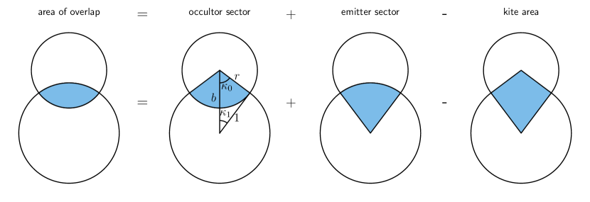
Figure 1: The area of overlap of two circles can be computed as the sum of the area of the sectors formed by the centers of each circle and the boundary between the points of intersection, minus the area of the kite-shaped region formed by the centers of the circles and the intersection points.   

Taking the radius of the larger circle to be unity, the standard formula for the lens-shaped overlap area is given by

$$A_{lens}=\pi\Lambda^{e}(r,b) =\begin{dcases}0&\qquad 1+r\leq b,\\ r^{2}\kappa_{0}+\kappa_{1}-\sqrt{\frac{4b^{2}-(1+b^{2}-r^{2})^{2}}{4}}&\qquad|1-r|<b<1+r,\\ \pi r^{2}&\qquad b\leq 1-r,\\ \pi&\qquad b\leq r-1,\\ \end{dcases}$$  (29)

(e.g. Mandel & Agol, 2002), where

$$\cos{\kappa_{0}} = \left(\frac{(r-1)(r+1)+b^{2}}{2br}\right),$$

$$\cos{\kappa_{1}} = \left(\frac{(1-r)(1+r)+b^{2}}{2b}\right),$$ (30)

and $\kappa_{0}$ and $\kappa_{1}$ are the angles defined in Figure 1. The second term in Equation (29) is the same as the standard formula for the area of overlap of two partially overlapping circles, with one of the circles scaled to a radius of unity (Weisstein, 2018). This term corresponds to ingress (and egress), it is the most expensive to compute, and it is most subject to numerical inaccuracy; we focus on this term in what follows.

We find that numerical round-off error limits the precision of the ingress formula when $b\approx 0$, $b+r\approx 1$, or $b\approx 1+r$; these are the cases in which the kite-shaped region becomes thin, in which the sum of two sides becomes similar in length to the spine of the kite. The square root term in this formula (Equation 29) computes the area of the kite-shaped region, which in this form causes round-off error when the kite is flattened. The same issue occurs when computing the area of a triangle in which two of the sides are of similar length; the kite has an area that is twice the area of the two mirror-image triangles connecting the centers of both circles and one of the intersection points. Goldberg (1991) gives a formula for precisely computing the area of a triangle, based on a method developed by William Kahan (later described in Kahan, 2000), which we use to compute the area of the kite-shaped region,

$$A_{kite} = \frac{1}{2}\sqrt{(A+(B+C))(C-(A-B))(C+(A-B))(A+(B-C))},$$ (31)

for $A\geq B\geq C$, where the tuple $\{A,B,C\}$ equals $\{1,r,b\}$ sorted from from greatest to least. Note that the order of operations needs to be carried out as specified by the series of parentheses in the entry to the square root; this sequence of operations preserves numerical precision. This formula is a novel implementation of Heron’s formula for a triangle for which loss of precision occurs due to subtracting quantities with similar numerical values which differ at high significant digits, and thus are more subject to round-off errors.

Next, the inverse cosine formulae are also imprecise when $\cos{\kappa_{0}}=x_{0}\approx 1$ or $\cos{\kappa_{1}}=x_{1}\approx 1$. The approximate solutions in this limit are $\kappa_{0}\approx[2(1-x_{0})]^{1/2}$ and $\kappa_{1}\approx[2(1-x_{1})]^{1/2}$, and so round-off error can occur both in taking the difference of two numbers close to unity, and in taking the square root.

Instead, we use the function $\theta=\mathrm{atan2}(y,x)$ with $y=\sin{\theta}$ and $x=\cos{\theta}$ to compute $\kappa_{0}$ and $\kappa_{1}$, which avoids the quadrant and division-by-zero problems of the $\theta=\tan^{-1}(y/x)$ function. In addition to the cosine values above, we require the sine terms, which are given by

$$\sin{\kappa_{0}} = \frac{A_{kite}}{br},$$

$$\sin{\kappa_{1}} = \frac{A_{kite}}{b},$$ (32)

which can be derived from the area of the triangles formed by the centers of the circles and one intersection point. Note that both $\sin{\kappa_{0}}$ and $\cos{\kappa_{0}}$ are divided by $br$, and $\sin{\kappa_{1}}$ and $\cos{\kappa_{1}}$ are divided by $b$, so that in the arctangent formula these denoninator terms cancel, which can improve numerical stability for small values of $b$ or $r$; this cancellation does not happen in the arccosine case given in Equation (3).

This results in the following equations for the overlap area, $A_{lens}$, of two partially overlapping circles:

$$A_{lens} =\kappa_{1}+r^{2}\kappa_{0}-A_{kite},$$

$$\kappa_{0} =\mathrm{atan2}(2A_{kite},(r-1)(r+1)+b^{2}),$$

$$\kappa_{1} =\mathrm{atan2}(2A_{kite},(1-r)(1+r)+b^{2}),$$  (33)

with $A_{kite}$ given in Equation (31).

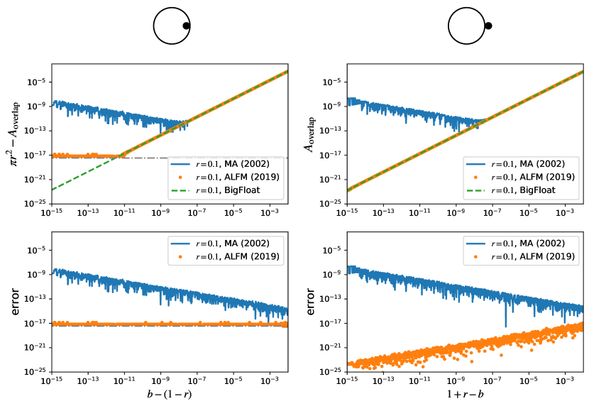
Figure 2: Precision of formulae for the area of overlap of two circles with radius ratio $r$. Plotted are the regions near $b=1-r$ (second and third points of contact) and $b=1+r$ (first and fourth points of contact) for the standard formula (Equation 29, blue) and our new formula (Equation 3, orange dots). The high-precision calculation is shown in green dashed for comparison; this is limited by the conversion of the result to double-precision. The solid and empty circles (top) indicate the positions of the circles at the left hand side of the axes. In the left panels the horizontal dash-dotted grey line indicates the limiting precision for representing $\pi r^{2}$.   

The performance of this formula relative to the standard formula is profiled in Figure 2 for $r=0.1$, a typical value for transiting exoplanets. We have carried out the computation in the Julia language, both in double-precision (Float64), and 256-bit precision (BigFloat), and subtracted the results to measure the numerical errors of the computation.

We find that the standard formula (Equation 29) approaches errors of $10^{-8}$ in the limit of $b\rightarrow 1-r$. This error exceeds the value of the area of the smaller circle minus the area of overlap for values of $1-r<b<1-r+10^{-8}$. Thus, even though this calculation is carried out in double precision, the precision achieved is of order single precision. Likewise, for $b\rightarrow 1+r$, the error of the standard formula approaches $10^{-8}$, with the error exceeding the value of the area of overlap for $1+r-10^{-8}<b<1+r$.

In contrast, Equation (3) gives a precision that is double-precision in both limits. Figure 2 shows that Equation (3) gives a precision of $\approx 10^{-17}$ in the limit $b\rightarrow 1-r$ for $r=0.1$; this limit is due to the limiting precision of representing $\pi r^{2}$ in double-precision, which in this case is $\pi r^{2}/2^{53}=10^{-17.4}$, indicated with a dash-dot grey line in the left hand panels of Figure 2. At the beginning of ingress/end of egress when $b\approx 1+r$, even higher precision is achieved since the area of overlap approaches zero, as shown in the right hand panels of Figure 2.

Finally, we compute the corresponding element of the solution vector $\mathfrak{s}_{0}$ as

$$\mathfrak{s}_{0}(r,b) = \pi-A_{lens}$$ (34)

$$= \pi-\kappa_{1}-r^{2}\kappa_{0}+A_{kite}.$$

We note that instead of computing $\kappa_{1}$, we compute $\pi-\kappa_{1}=-\mathrm{atan2}(\sin{\kappa_{1}},\cos{\kappa_{1}})$, which leads to double precision as well. Note also that $\mathfrak{s}_{0}$ is identical to the first basis function ($s_{0}$) in the starry implementation from Luger et al. (2019a).

3.1 Derivatives

The partial derivatives of this formula with respect to the radius ratio, $r$, and impact parameter, $b$, turn out to be straightforward:

$$\frac{\partial\mathfrak{s}_{0}(r,b)}{\partial r} =-2r\kappa_{0},$$

$$\frac{\partial\mathfrak{s}_{0}(r,b)}{\partial b} =\frac{2A_{kite}}{b},$$  (35)

which can be computed from the quantities already used in calculating $\mathfrak{s}_{0}$. At the contact points, when $b=|1\pm r|$, the derivatives are undefined. In practice this can be a problen when taking finite-differences across the discontinuous boundary, but with the analytic formulae, these points are a set of measure zero, and so we simply set the derivatives to zero at these points.

In the remainder of this paper we will need to use these formulae in computing the higher order limb-darkened light curves. In the next section, we revisit the formulae for linear limb darkening.

4 Linear limb darkening

We now turn to the case of linear limb darkening, $I(\upmu)/I_{0}=1-u_{1}(1-\upmu)$ (Russell & Shapley, 1912a, b). In this section we set $I_{0}=1$ and $u_{1}=1$, so that $I(\upmu)=\upmu$, which corresponds to the $n=1$ terms in both the polynomial and Green’s bases; the general linear limb-darkening case can be computed as a linear combination with the uniform case. Note that since $\upmu=\sqrt{1-x^{2}-y^{2}}$, this problem is equivalent to computing the volume of intersection between a sphere and a cylinder, which was solved in terms of elliptic integrals by Lamarche & Leroy (1990). A similar solution was found by Mandel & Agol (2002), who show that the total flux visible during the occultation of a body whose surface map is given by $I(x,y)=\sqrt{1-\mbox{$x$}^{2}-\mbox{$y$}^{2}}$ may be computed as

$$\mathfrak{s}_{1}=\frac{2\pi}{3}\left(1-\frac{3\Lambda(r,b)}{2}-\Theta(r-b)\right)$$ (36)

where $\Theta(\scaleto{\cdot}{6pt})$ is the Heaviside step function and

$$\Lambda(r,b) =\begin{dcases}\frac{1}{9\pi\sqrt{br}}\Bigg{[}\frac{(r+b)^{2}-1}{r+b}\Big{(}-2r\,\big{(}2(r+b)^{2}+(r+b)(r-b)-3\big{)}K(k^{2})&\\ \phantom{XXXX}+3(b-r)\,\Pi\big{(}k^{2}(b+r)^{2},\,k^{2}\big{)}\Big{)}-4br(4-7r^{2}-b^{2})E(k^{2})\Bigg{]}&\qquad k^{2}<1\\[15.00002pt] \frac{2}{9\pi}\Bigg{[}\big{(}1-(r+b)^{2}\big{)}\Bigg{(}\sqrt{1-(b-r)^{2}}\,K\left(\frac{1}{k^{2}}\right)+3\left(\frac{b-r}{(b+r)\sqrt{1-(b-r)^{2}}}\right)&\\ \phantom{XX}\times\Pi\left(\frac{1}{k^{2}(b+r)^{2}},\,\frac{1}{k^{2}}\right)\Bigg{)}-\sqrt{1-(b-r)^{2}}(4-7r^{2}-b^{2})E\left(\frac{1}{k^{2}}\right)\Bigg{]}&\qquad k^{2}\geq 1\end{dcases}$$  (37)

with

$$k^{2} =\frac{1-r^{2}-b^{2}+2br}{4br}\hskip 0.0pt.$$ (38)

Note that $\mathfrak{s}_{1}(r,b)=s_{2}(r,b)$ in the spherical harmonic expansion used in starry as described in Luger et al. (2019a). For the cases $b=r$, $b=1-r$, $b=0$, $r=0$, or $|r-b|\geq 1$, there are special expressions for $\Lambda(r,b)$ given below. In the expressions above, $K(\scaleto{\cdot}{6pt})$, $E(\scaleto{\cdot}{6pt})$, and $\Pi(\scaleto{\cdot}{6pt},\scaleto{\cdot}{6pt})$ are the complete elliptic integrals of the first, second kind, and third kind, respectively, defined as

$$K(k^{2}) \equiv\int_{0}^{\frac{\pi}{2}}\frac{\mathrm{d}\varphi}{\sqrt{1-k^{2}\sin^{2}\varphi}}$$

$$E(k^{2}) \equiv\int_{0}^{\frac{\pi}{2}}\sqrt{1-k^{2}\sin^{2}\varphi}\,\mathrm{d}\varphi$$

$$\Pi(n,k^{2}) \equiv\int_{0}^{\frac{\pi}{2}}\frac{\mathrm{d}\varphi}{(1-n\sin^{2}\varphi)\sqrt{1-k^{2}\sin^{2}\varphi}}\hskip 0.0pt.$$ (39)

In Equation (37) we have transformed the formulae from Mandel & Agol (2002) using Equation (17.7.17) from Abramowitz & Stegun (1970) which yields equations that are better behaved in the vicinity of $b=r$. However, these elliptic integrals are still subject to numerical instability as $r\rightarrow 1-b$ and $r\gg 1$. The main issue is the logarithmic divergence of $K$ and $\Pi$ as $k\rightarrow 1$, as well as numerical cancellations leading to round-off errors which occur in the limit $k\rightarrow 0$.

Through trial and error, we have found that these instabilities can be removed by combining elliptic integrals into a general complete elliptic integral defined by Bulirsch (1969) as

$$\mathrm{cel}(k_{c},p,a,b)=\int_{0}^{\pi/2}\frac{a\cos^{2}{\phi}+b\sin^{2}{\phi}}{\cos^{2}{\phi}+p\sin^{2}{\phi}}\frac{d\phi}{\sqrt{\cos^{2}{\phi}+k_{c}^{2}\sin^{2}{\phi}}},$$ (40)

where $k_{c}=\sqrt{1-m_{k}}$, and for $b+r\geq 1$, $m_{k}=k^{2}$, while for $b+r\leq 1$, $m_{k}=1/k^{2}$. The derivatives of $\mathrm{cel}$ with respect to the input parameters are given in Appendix B. Although $k_{c}$ can be computed from $m_{k}$, we have found better numerical stability in computing $k_{c}$ analytically from $b$ and $r$:

$$k_{c} =\begin{dcases}\sqrt{\frac{(b+r)^{2}-1}{4br}}&\qquad k^{2}\leq 1\\ \sqrt{\frac{1-(b+r)^{2}}{1-(b-r)^{2}}}&\qquad k^{2}>1.\end{dcases}$$ (41)

In practice, we let the subroutine that computes $\mathrm{cel}$ accept both $m_{k}$ and $k_{c}$ as input for numerical precision.

To transform the elliptic integrals in Equation (37) to $\mathrm{cel}$, we used the following relations from Bulirsch (1969):

$$\lambda K(m_{k})+qE(m_{k}) = {\rm cel}(k_{c},1,\lambda+q,\lambda+qk_{c}^{2})$$ (42)

$$\lambda K(m_{k})+q\Pi(n,m_{k}) = {\rm cel}(k_{c},1-n,\lambda+q,\lambda(1-n)+q)$$ (43)

$$E(m_{k}) = {\rm cel}(k_{c},1,1,1-m_{k})$$ (44)

$$E(m_{k})-(1-m_{k})K(m_{k}) = m_{k}\,{\rm cel}(k_{c},1,1,0)$$ (45)

$$\Pi(n,m_{k})-K(m_{k}) = n\,{\rm cel}(k_{c},1-n,0,1),$$ (46)

noting that Bulirsch (1969) uses a different sign convention for $\Pi(n,m_{k})$. In particular, the expressions for $\Pi(n,m_{k})-K(m_{k})$ and $E(m_{k})-(1-m_{k})K(m_{k})$ are useful for eliminating the singularities and cancellations which occur at $m_{k}=1$ when $b+r=1$ and $m_{k}=0$ when $r\rightarrow\infty$. The general complete elliptic integral is evaluated with the approach of Bartky (1938), which uses recursion to approximate the integral to a specified precision.

These elliptic integral transformations lead to the following numerically-stable expression for the linear limb darkening flux, $\mathfrak{s}_{1}(r,b)$, in which

$$\Lambda =\begin{dcases}0&\qquad r=0\\ 0&\qquad|r-b|\geq 1\\ -\tfrac{2}{3}(1-r^{2})^{3/2}&\qquad b=0\\ \tfrac{1}{3}-\tfrac{4}{9\pi}&\qquad b=r=\tfrac{1}{2}\\ \tfrac{1}{3}+\tfrac{2}{9\pi}{\rm cel}\left(k_{c},1,m_{k}-3,(1-m_{k})(2m_{k}-3)\right)&\qquad b=r<\tfrac{1}{2}\\ \tfrac{1}{3}+\tfrac{4r}{9\pi}{\rm cel}\left(k_{c},1,1-3m_{k},m_{k}-1\right)&\qquad b=r>\tfrac{1}{2}\\ \tfrac{2}{9\pi}\left[3\cos^{-1}(1-2r)-2(3+2r-8r^{2})\sqrt{rb}-3\pi\Theta(r-\tfrac{1}{2})\right]&\qquad b+r=1\\ \frac{1-(b-r)^{2}}{9\pi\sqrt{br}}\Bigg{[}\frac{(b+r)^{2}-1}{4br}(b^{2}-r^{2}){\rm cel}(k_{c},(b-r)^{2}(1-m_{k}),0,3)&\\ \phantom{XXXX}-(3-6r^{2}-2br){\rm cel}(k_{c},1,1,0)-4brE(m_{k})\Bigg{]}&\qquad k^{2}<1\\[15.00002pt] \frac{2\sqrt{1-(b-r)^{2}}}{9\pi}\Bigg{[}\big{(}1-(r+b)^{2}\big{)}{\rm cel}(k_{c},p,1+q,p+q)&\\ \phantom{XXXX}-(4-7r^{2}-b^{2})E\left(m_{k}\right)\Bigg{]}&\qquad k^{2}>1\\ \end{dcases}$$  (47)

where

$$q = 3\frac{b-r}{(b+r)(1-(b-r)^{2})}$$

$$p = \left(\frac{b-r}{b+r}\right)^{2}\frac{1-(b+r)^{2}}{1-(b-r)^{2}}$$ (48)

in the $k^{2}>1$ case. Note that in this equation the conditions should be evaluated in the order they appear.

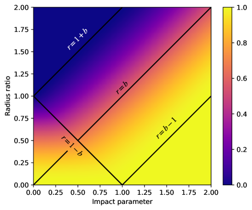
Figure 3: The flux of a linearly limb-darkened star being eclipsed, $F=\tfrac{3}{2\pi}\mathfrak{s}_{1}(r,b)$, with $u_{1}=1$ (all other $u_{n}$ zero), for which $I_{0}=3/(2\pi)$. In the limit $b>r+1$, no eclipse occurs, so $F=1$. For $b<r-1$, the star is completely eclipsed and $F=0$. In the limits $b=r$ and $b=1-r$, special expressions must be used.   

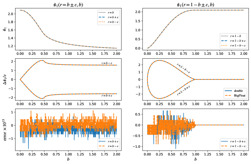
Figure 4: The accuracy of $\mathfrak{s}_{1}(r,b)$ near $b=r$ (left panels) and $b=1-r$ (right panels) for $\epsilon=10^{-8}$. The $x$-axes are impact parameter $b$, while the $y$ axes in the top panels show $\mathfrak{s}_{1}(r,b)$, with $r$ given in the legend of each panel. The middle panels plot the difference $(\mathfrak{s}_{1}(b\pm\epsilon,b)-\mathfrak{s}_{1}(b,b))/\epsilon$ and $(\mathfrak{s}_{1}(1-b\pm\epsilon,b)-\mathfrak{s}_{1}(1-b,b))/\epsilon$. The bottom panels show the numerical precision by the comparing double precision computation with BigFloat precision (256-bit).   

The $\mathfrak{s}_{1}(r,b)$ function is plotted in Figure 3. The function varies smoothly from the lower right where the disk is unocculted to the upper left where it is completely occulted. There are several points which need to be handled separately as the Equation (37) expressions become singular or are no longer valid; the solid lines in Figure 3 show these points. When $b=0$, the integral over the center of the disk simplifies greatly. When $b=r=1/2$, at the intersection of $b=r$ and $b=1-r$, another simplification occurs. For $b=r$, the disk of the occultor crosses the center of the source; this needs to be computed separately in the $r<1/2$, $r=1/2$, and $r>1/2$ limits. The first and fourth contacts occur at $b=1+r$, where $\mathfrak{s}_{1}=1$; this is the upper bound to the $k^{2}<1$ region for $b+r>1$. For $r\geq 1$, the second and third contacts (at the start and end of complete occultation) occur when $b=1-r$, which is the lower bound to the $k^{2}<1$ region when $b+r>1$. For $r<1$, the second and third contacts occur when $r=1-b$.

Near these boundaries, the standard Mandel & Agol (2002) expressions can become singular, and so we paid particular care to the accuracy of these new expressions in these regions. Figure 4 shows that Equation (47) is accurate to double precision in all of these regimes. We tested the accuracy by computing the equations with 256 bit arithmetic, which is much less subject to round-off error, and hence gives more precise expressions than double precision. We implemented the pseudocode from Bulirsch (1969) to compute ${\rm cel}(k_{c},p,a,b)$, which has a termination test that scales as the square root of the double precision. We find that the transformed expressions are accurate to $\sim 10^{-14}$ when computed in double precision within $\epsilon=10^{-8}$ of the vicinity of $b=r$ and $b=1-r$.

Finally, in Figures 5 and 6 we plot the relative numerical error in the flux of a linearly limb-darkened source when using the equations in Mandel & Agol (2002) and in this paper, respectively, over a portion of the $b-r$ plane. The former method (Figure 5) yields errors on the order of $10^{-7}$ over most of the domain, although the error approaches unity near the singular regions discussed above. In contrast, the method introduced in this paper (Figure 6; note the change in the color scale) yields errors close to double precision everywhere, including the vicinity of the singular points.

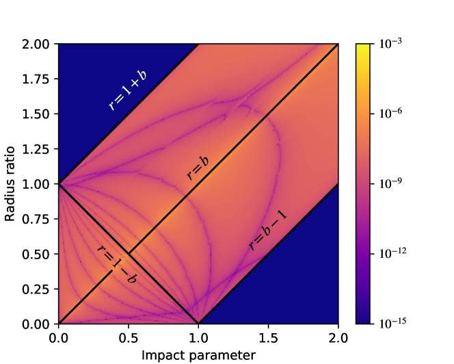
Figure 5: The numerical error in computing the flux of an eclipsed, linearly limb-darkened star ($u_{1}=1$) using the equations in Mandel & Agol (2002).   

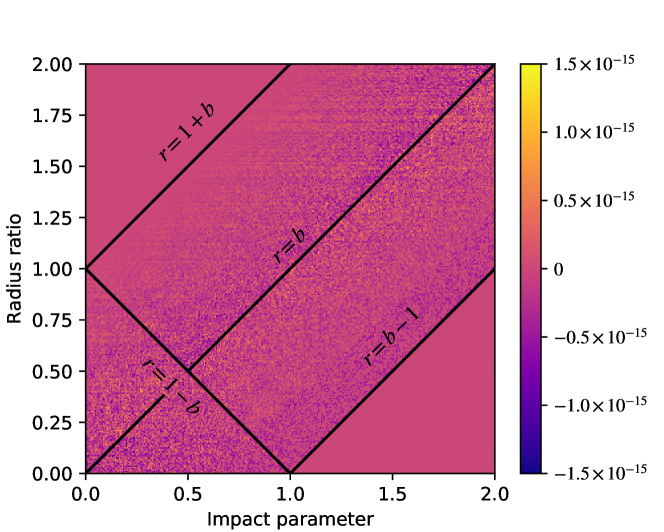
Figure 6: The numerical error in computing the flux of an eclipsed, linearly limb-darkened star ($u_{1}=1$) using the $\mathfrak{s}_{1}(r,b)$ formalism introduced in this paper. Compare to Figure 5, noting the change in the color scale. The new method is eight orders of magnitude more precise on average, approaching double precision accuracy everywhere in the domain.   

4.1 Derivatives

The derivatives of $\Lambda$ with respect to $r$ and $b$ are:

$$\frac{\partial\Lambda}{\partial r} =\begin{dcases}0\phantom{MMMMMMMMMMMMMMMMMMM}&\qquad r=0\\ 0&\qquad|r-b|\geq 1\\ 2r\sqrt{1-r^{2}}&\qquad b=0\\ \frac{2}{\pi}&\qquad b=r=\tfrac{1}{2}\\ \frac{4r}{\pi}E(4r^{2})&\qquad b=r<\tfrac{1}{2}\\ \frac{2}{\pi}\mathrm{cel}(k_{c},1,1,0)&\qquad b=r>\tfrac{1}{2}\\ \frac{8r}{\pi}\sqrt{r(1-r)}&\qquad b+r=1\\ \frac{8br^{2}E(k^{2})+2r(1-(b+r)^{2})K(k^{2})}{\pi\sqrt{br}}&\\ \phantom{XX}=\frac{1}{\pi\sqrt{br}}\mathrm{cel}(k_{c},1,2r(1-(b-r)^{2}),0)&\qquad k^{2}<1\\[15.00002pt] \frac{4r}{\pi}\sqrt{1-(b-r)^{2}}E(k^{-2})&\\ \phantom{XX}=\frac{4r}{\pi}\sqrt{1-(b-r)^{2}}\mathrm{cel}(k_{c},1,1,k_{c}^{2})&\qquad k^{2}>1\\ \end{dcases}$$  (49)

and

$$\frac{\partial\Lambda}{\partial b} =\begin{dcases}0&\qquad r=0\\ 0&\qquad|r-b|\geq 1\\ 0&\qquad b=0\\ -\frac{2}{3\pi}&\qquad b=r=\tfrac{1}{2}\\ \frac{4r}{3\pi}\mathrm{cel}(k_{c},1,-1,k_{c}^{2})&\qquad b=r<\tfrac{1}{2}\\ -\frac{2}{3\pi}\mathrm{cel}(k_{c},1,1,2k_{c}^{2})&\qquad b=r>\tfrac{1}{2}\\ -\frac{8r}{3\pi}\sqrt{r(1-r)}&\qquad b+r=1\\ \frac{4r(r^{2}+b^{2}-1)E(k^{2})+2r(1-(b+r)^{2})K(k^{2})}{3\pi\sqrt{br}}&\\ \phantom{XX}=\frac{1-(b-r)^{2}}{3\pi\sqrt{br}}\mathrm{cel}(k_{c},1,-2r,(1-(b+r)^{2})/b)&\qquad k^{2}<1\\[15.00002pt] \frac{2}{3b\pi}\sqrt{1-(b-r)^{2}}\left[(r^{2}+b^{2}-1)E(k^{-2})+(1-(b+r)^{2})K(k^{-2})\right]&\\ \phantom{XX}=\frac{4r}{3\pi}\sqrt{1-(b-r)^{2}}\mathrm{cel}(k_{c},1,-1,k_{c}^{2})&\qquad k^{2}>1,\\ \end{dcases}$$  (50)

where we have given some of the expressions in terms of both the standard elliptic integrals and the general elliptic integral.

From these expressions, the derivatives of $\mathfrak{s}_{1}$ are given by

$$\frac{\partial\mathfrak{s}_{1}}{\partial r} = -\pi\frac{\partial\Lambda}{\partial r},$$ (51)

$$\frac{\partial\mathfrak{s}_{1}}{\partial b} = -\pi\frac{\partial\Lambda}{\partial b}.$$ (52)

We have tested these formulae with finite-difference derivatives evaluated at 256-bit precision, and, as with the total flux term, we find that these are accurate to $\lesssim 2\times 10^{-15}$, close to double precision.

We next increase the power of limb darkening by one, $\upmu^{2}$.

5 Quadratic limb darkening

The next order of limb darkening has been widely studied due to its accurate description of stellar atmospheres (Claret, 2000; Mandel & Agol, 2002; Pál, 2008). We summarize here the formulae for quadratic limb darkening for $I(\upmu)=4\upmu^{2}-2$, along with the derivatives, using the transformed expressions described above. The general quadratic case may be computed as a linear combination with the foregoing uniform and linear cases.

We first give the formula for the function $\eta(r,b)$, which is the term appearing in the quadratic limb darkening model only when $u_{2}\neq 0$ (Mandel & Agol, 2002). In terms of quantities we have defined above for the uniform case:

$$\eta(r,b) =\begin{dcases}\frac{1}{2\pi}\left[\kappa_{1}+r^{2}(r^{2}+2b^{2})\kappa_{0}-\frac{1}{2}(1+5r^{2}+b^{2})A_{kite}\right]&\qquad k^{2}\leq 1\\[15.00002pt] \frac{r^{2}}{2}(r^{2}+2b^{2})&\qquad k^{2}>1\\ \end{dcases}$$  (53)

As $\kappa_{0}$, $\kappa_{1}$, and $A_{kite}$ were already computed in the uniform case, these quantities are reused in the quadratic computation.

With this definition, the quadratic term, $\mathfrak{s}_{2}(r,b)$ is given simply by

$$\mathfrak{s}_{2} = 2\mathfrak{s}_{0}+4\pi\eta-2\pi\hskip 0.0pt,$$ (54)

where $\mathfrak{s}_{0}$ is defined in Equation (34).

5.1 Derivatives

The derivatives of $\eta$ are given by:

$$\frac{\partial\eta}{\partial r} =\begin{dcases}\frac{2r}{\pi}\left[(r^{2}+b^{2})\kappa_{0}-2A_{kite}\right]&\qquad k^{2}\leq 1\\[15.00002pt] 2r(r^{2}+b^{2})&\qquad k^{2}>1\\ \end{dcases}$$  (55)

and

$$\frac{\partial\eta}{\partial b} =\begin{dcases}\frac{1}{2b\pi}\left[4r^{2}b^{2}\kappa_{0}-2(1+b^{2}+r^{2})A_{kite}\right]&\qquad k^{2}\leq 1\\[15.00002pt] 2br^{2}&\qquad k^{2}>1\\ \end{dcases}$$  (56)

where the derivatives of $\mathfrak{s}_{0}$ are defined in Equation (3.1). The derivatives of the $\mathfrak{s}_{2}$ term are thus

$$\frac{\partial\mathfrak{s}_{2}}{\partial r} = 2\frac{\partial\mathfrak{s}_{0}}{\partial r}+4\pi\frac{\partial\eta}{\partial r},$$

$$\frac{\partial\mathfrak{s}_{2}}{\partial b} = 2\frac{\partial\mathfrak{s}_{0}}{\partial b}+4\pi\frac{\partial\eta}{\partial b}\hskip 0.0pt.$$ (57)

In the following section we turn our attention to the general polynomial limb darkening case, $\upmu^{n}$ with $n>2$. As discussed in Luger et al. (2019a), these terms may be expressed exactly as the sum of spherical harmonics with $m=0$. However, it is possible to exploit the azimuthal symmetry of the limb darkening problem to derive far more efficient and accurate formulae, which we describe in the following section.

6 Higher Order Limb Darkening

Having computed $\mathfrak{s}_{0}$, $\mathfrak{s}_{1}$, and $\mathfrak{s}_{2}$, we now seek a general expression for $\mathfrak{s}_{n}$ for any $n>2$. Recalling our definition of $\mathfrak{s}$ as the surface integral of the terms in the Green’s basis,

$$\mathfrak{s}\equiv\iint\tilde{\mathfrak{g}}(z)\,\mathrm{d}S\hskip 0.0pt,$$ (58)

in this section we will use Green’s theorem to re-express this two-dimensional integral as a one-dimensional line integral over the boundary of the visible portion of the occulted body’s disk. This is the same procedure adopted by Luger et al. (2019a), albeit with different basis functions. Given ${\mathbf{r}}=x\mathbf{\hat{x}}+y\mathbf{\hat{y}}$, we may write

$$\mathfrak{s} =\oint{\mathbf{G}}(z)\cdot\mathrm{d}{\mathbf{r}}\hskip 0.0pt,$$ (59)

where ${\mathbf{G}}$ is a matrix whose $n^{\mathrm{th}}$ row is the vector

$${\mathbf{G}}_{n}(z)=G_{n,x}(z)\,\mathbf{\hat{x}}+G_{n,y}(z)\,\mathbf{\hat{y}}\hskip 0.0pt.$$ (60)

The components $G_{n,x}$ and $G_{n,y}$ are chosen such that

$${\mathbf{D}}\wedge{\mathbf{G}}_{n} \equiv\frac{\mathrm{d}G_{n,y}}{\mathrm{d}\mbox{$x$}}-\frac{\mathrm{d}G_{n,x}}{\mathrm{d}\mbox{$y$}}$$

$$=\tilde{\mathfrak{g}}_{n}(z)\hskip 0.0pt.$$ (61)

As in Pál (2012) and Luger et al. (2019a), the operation ${\mathbf{D}}\wedge{\mathbf{G}}_{n}$ denotes the exterior derivative of ${\mathbf{G}}_{n}$. Following Luger et al. (2019a), if we choose the following form for Equation (60),

$$\mathbf{G}_{n}(z)=z^{n}(-y\mathbf{\hat{x}}+x\mathbf{\hat{y}})\hskip 0.0pt,$$ (62)

we arrive at the expression presented in Equation (14) for the components of the Green’s basis:

$$\tilde{\mathfrak{g}}_{n}(z) =\frac{\mathrm{d}{G_{n}}_{y}}{\mathrm{d}\mbox{$x$}}-\frac{\mathrm{d}{G_{n}}_{x}}{\mathrm{d}\mbox{$y$}}$$

$$=(n+2)z^{n}-nz^{n-2}$$ (63)

for $2\leq n\leq N$. Note that we already introduced the first three terms, $\tilde{\mathfrak{g}}_{0}=1$ (uniform limb darkening), $\tilde{\mathfrak{g}}_{1}=z$ (linear limb darkening), and $\tilde{\mathfrak{g}}_{2}=4z^{2}-2$ (quadratic limb darkening). Since we already know how to integrate them (§3–5), we treat them separately from the higher order terms.

Returning to Equation ((LABEL:greens)), we note that the line integral consists of two arcs: an arc $\mathcal{P}$ along the boundary of the occulting body and an arc $\mathcal{Q}$ along the boundary of the occulted body. We may therefore write the $n^{\mathrm{th}}$ component of the solution vector as

$$\mathfrak{s}_{n} =\mathcal{Q}({\mathbf{G}}_{n})-\mathcal{P}({\mathbf{G}}_{n})\hskip 0.0pt,$$ (64)

where, as in Pál (2012) and Luger et al. (2019a), we define the primitive integrals

$$\mathcal{P}({\mathbf{G}}_{n}) \equiv\int\displaylimits_{\pi-\phi}^{2\pi+\phi}\big{[}G_{n,y}(rc_{\varphi},b+rs_{\varphi})c_{\varphi}-G_{n,x}(rc_{\varphi},b+rs_{\varphi})s_{\varphi}\big{]}r\mathrm{d}\varphi\hskip 0.0pt,$$ (65)

taken along the boundary of the occulting body of radius $$r$$, and

$$\mathcal{Q}({\mathbf{G}}_{n}) \equiv\int\displaylimits_{\pi-\lambda}^{2\pi+\lambda}\big{[}G_{n,y}(c_{\varphi},s_{\varphi})c_{\varphi}-G_{n,x}(c_{\varphi},s_{\varphi})s_{\varphi}\big{]}\mathrm{d}\varphi\hskip 0.0pt,$$ (66)

taken along the boundary of the occulted body of radius unity. For convenience, we defined $c_{\varphi}\equiv\cos\varphi$ and $s_{\varphi}\equiv\sin\varphi$ and we used the fact that along the arc of a circle,

$$\mathrm{d}{\mathbf{r}} =-rs_{\varphi}\,\mathrm{d}\varphi\,\mathbf{\hat{x}}+rc_{\varphi}\,\mathrm{d}\varphi\,\mathbf{\hat{y}}\hskip 0.0pt.$$ (67)

The angles $\phi$ and $\lambda$ are the same as those used in Luger et al. (2019a) (see their Figure 2) and are given by $\phi=\kappa_{0}-\pi/2$ and $\lambda=\pi/2-\kappa_{1}$ (c.f. Equation 3 and Figure 1).

Inserting our expression for $\mathbf{G}_{n}$ into Equations (65) and (66), we arrive at a fairly simple form for the primitive integrals:

$$\mathcal{P}({\mathbf{G}}_{n}) =\int\displaylimits_{\pi-\phi}^{2\pi+\phi}z^{n}(r+b\sin{\varphi})rd\varphi$$ (68)

and

$$\mathcal{Q}({\mathbf{G}}_{n}) =\int\displaylimits_{\pi-\lambda}^{2\pi+\lambda}z^{n}d\varphi\hskip 0.0pt.$$ (69)

Conveniently, the primitive integral $\mathcal{Q}({\mathbf{G}}_{n})=0$ for all $n>0$, since $z=0$ at the boundary of the star. Since we need not compute the integral for $n=0$, as we already found a solution for uniform limb darkening in §3, our final task is to find the solution to Equation (68).

6.1 Solving the $\mathcal{P}$ integral

The primitive integral $\mathcal{P}({\mathbf{G}}_{n})$ can be rewritten as

$$\mathcal{P}({\mathbf{G}}_{n})=\int_{\pi-\phi}^{2\pi+\phi}\left(1-r^{2}-b^{2}-2brs_{\varphi}\right)^{\frac{n}{2}}(r+bs_{\varphi})rd\varphi,$$ (70)

where $s_{\varphi}=\sin{\varphi}$. We make the transformation $\xi=\tfrac{1}{2}\left(\varphi-\tfrac{3\pi}{2}\right)$, yielding

$$\mathcal{P}({\mathbf{G}}_{n})=2r(4br)^{\frac{n}{2}}\int\displaylimits_{-\tfrac{\kappa_{0}}{2}}^{\tfrac{\kappa_{0}}{2}}(k^{2}-\sin^{2}\xi)^{\tfrac{n}{2}}(r-b+2b\sin^{2}\xi)d\xi,$$ (71)

for $2\leq n\leq N$, where $\kappa_{0}=2\sin^{-1}k$ for $k^{2}\leq 1$ and $\kappa_{0}=\pi$ for $k^{2}>1$. We reuse the value of $\kappa_{0}$ which was computed in the uniform limb darkening case (§3).

We can express $\mathcal{P}({\mathbf{G}}_{n})$ in terms of a sequence of integrals, $\mathcal{M}_{n}(r,b)$, given by:

$$\mathcal{M}_{n}(r,b)=(4br)^{n/2}\int_{-\kappa_{0}/2}^{\kappa_{0}/2}(k^{2}-\sin^{2}\xi)^{\tfrac{n}{2}}d\xi,$$ (72)

in terms of which the primitive integral takes the particulary simple form

$$\mathcal{P}({\mathbf{G}}_{n})=(1+r^{2}-b^{2})\mathcal{M}_{n}-\mathcal{M}_{n+2}.$$  (73)

The integrals $\mathcal{M}_{n}$ obey straightforward recursion relations

$$\mathcal{M}_{n} =\frac{1}{n}\left[2(n-1)(1-r^{2}-b^{2})\mathcal{M}_{n-2}\right.$$

$$+\left.(n-2)(1-(b-r)^{2})((b+r)^{2}-1)M_{n-4}\right],$$  (74)

$$\mathcal{M}_{n} =\frac{(n+4)\mathcal{M}_{n+4}-2(n+3)(1-r^{2}-b^{2})\mathcal{M}_{n+2}}{(n+2)(1-(b-r)^{2})((b+r)^{2}-1)},$$  (75)

where the first relation may be used for upwards recursion in $n$ for $k^{2}>\frac{1}{2}$, and the second for downward recursion in $n$ otherwise. In practice we replace $\mathcal{M}_{n+2}$ in Equation (73) with the recursion relation to obtain a more stable expression for $\mathcal{P}({\mathbf{G}}_{n})$:

$$\mathcal{P}({\mathbf{G}}_{n})=2r^{2}\mathcal{M}_{n}-\frac{n}{n+2}\left((1-r^{2}-b^{2})\mathcal{M}_{n}+(1-(b-r)^{2})((b+r)^{2}-1)\mathcal{M}_{n-2}\right).$$  (76)

Note that these recursion relations involve every fourth term, so we need to compute the first four terms analytically. These are given by:

$$\mathcal{M}_{0} =\kappa_{0},$$

$$\mathcal{M}_{1} =2(4br)^{1/2}\left[E(k^{2})-(1-k^{2})K(k^{2})\right],$$

$$\mathcal{M}_{2} =4br\left[(k^{2}-\tfrac{1}{2})\kappa_{0}+k\sqrt{1-k^{2}}\right],$$

$$\mathcal{M}_{3} =\tfrac{2}{3}(4br)^{3/2}\left[(4k^{2}-2)E(k^{2})+(3k^{2}-2)(k^{2}-1)K(k^{2})\right],$$  (77)

for $k^{2}\leq 1$, while for $k^{2}>1$,

$$\mathcal{M}_{0} =\pi,$$

$$\mathcal{M}_{1} =2(1-(r-b)^{2})^{1/2}E(k^{-2}),$$

$$\mathcal{M}_{2} =\pi(1-b^{2}-r^{2}),$$

$$\mathcal{M}_{3} =\tfrac{2}{3}(4br)^{3/2}k^{3}\left[2(2-k^{-2})E(k^{-2})-(1-k^{-2})K(k^{-2})\right].$$  (78)

We re-express the elliptic integrals for $n=1$ and $n=3$ in terms of the cel integrals which were already computed for the linear limb darkening case,

$$\mathcal{M}_{1} =2(4br)^{1/2}k^{2}\mathrm{cel}(k_{c},1,1,0),$$

$$\mathcal{M}_{3} =\tfrac{2}{3}(4br)^{3/2}k^{2}\left[\mathrm{cel}(k_{c},1,1,k_{c}^{2})+(3k^{2}-2)\mathrm{cel}(k_{c},1,1,0)\right],$$  (79)

for $k^{2}\leq 1$, while for $k^{2}>1$,

$$\mathcal{M}_{1} =2(1-(r-b)^{2})^{1/2}\mathrm{cel}(k_{c},1,1,k_{c}^{2}),$$

$$\mathcal{M}_{3} =\tfrac{2}{3}(1-(b-r)^{2})^{3/2}\left[(3-2k^{-2})\mathrm{cel}(k_{c},1,1,k_{c}^{2})+k^{-2}\mathrm{cel}(k_{c},1,1,0\right].$$  (80)

where, as before, $k_{c}=\sqrt{1-k^{2}}$ for $k^{2}\leq 1$, and $k_{c}=\sqrt{1-k^{-2}}$ for $k^{2}>1$.

For downward recursion, we compute the top four $\mathcal{M}_{n}$ expressions, $N-3\leq n\leq N$, in terms of series expansions. When $k^{2}\leq 1$, the integrals may be expressed in terms of the following Hypergeometric functions and infinite series,

$$\mathcal{M}_{n} =(4br)^{n/2}k^{n+1}\pi^{1/2}\frac{\Gamma{(1+\tfrac{n}{2})}}{\Gamma(\tfrac{3}{2}+\tfrac{n}{2})}\,_{2}F_{1}(\tfrac{1}{2},\tfrac{1}{2};\tfrac{3}{2}+\tfrac{n}{2};k^{2}),$$

$$=(1-(r-b)^{2})^{n/2}k\sum_{j=0}^{j_{max}}\alpha_{j}k^{2j},$$

$$\alpha_{0} =\sqrt{\pi}\frac{\Gamma(1+\tfrac{n}{2})}{\Gamma(\tfrac{3}{2}+\tfrac{n}{2})},$$

$$\alpha_{j} =\alpha_{j-1}\frac{(2j-1)^{2}}{2j(1+n+2j)}.$$  (81)

Although $j_{max}=\infty$, in practice we set $j_{max}=100$, and the series is truncated when a term goes below a tolerance specified by the numerical precision.

We find that upward recursion in $n$ is more stable for $k^{2}>\tfrac{1}{2}$, while downward recursion is more stable for $k^{2}<\tfrac{1}{2}$. Note that this differs from Luger et al. (2019a), for which downward recursion was also required for $k^{2}>2$.

6.2 Analytic derivatives

The derivatives of $\mathcal{P}({\mathbf{G}}_{n})$ may be expressed simply as functions of $\mathcal{M}_{n}$:

$$\frac{\partial\mathcal{P}}{\partial r} = 2r\left[(n+2)\mathcal{M}_{n}-n\mathcal{M}_{n-2}\right],$$ (82)

$$\frac{\partial\mathcal{P}}{\partial b} = \frac{n}{b}\left[(r^{2}+b^{2})(\mathcal{M}_{n}-\mathcal{M}_{n-2})+(r^{2}-b^{2})^{2}\mathcal{M}_{n-2}\right].$$ (83)

Since the $\mathcal{M}_{n}$ integrals are computed for the total flux case, there is little overhead for computing the derivatives.

For small values of $b$ we find that the derivative with respect to impact parameter becomes numerically unstable due to the near cancellation between the two terms, followed by division by $b$. To avoid this problem for small $b$, we have derived an alternative expression which avoids division by $b$ which we utilize when $b<b_{c}$, where $b_{c}$ is a (small) cutoff value:

$$\frac{\partial\mathcal{P}}{\partial b}=n\left[b\mathcal{M}_{n}+(2r^{3}+b^{3}-3r^{2}b-b-3)\mathcal{M}_{n-2}-4r^{3}\mathcal{N}_{n-2}\right],$$ (84)

where we have defined a new integral, $\mathcal{N}_{n}$,

$$\mathcal{N}_{n}(r,b)=(4br)^{n/2}\int_{-\kappa_{0}/2}^{\kappa_{0}/2}(k^{2}-\sin^{2}\xi)^{\tfrac{n}{2}}\sin^{2}{\xi}d\xi,$$ (85)

which obeys the recursion relation

$$\mathcal{N}_{n}=\frac{1}{n+2}\left[\mathcal{M}_{n}+n(1-(b+r)^{2})\mathcal{N}_{n-2}\right].$$  (86)

Since this recursion relation involves every other term, we only need the two lowest terms, which are given by:

$$\mathcal{N}_{0} =\tfrac{1}{2}\kappa_{0}-kk_{c},$$

$$\mathcal{N}_{1} =\tfrac{2}{3}(4br)^{1/2}k^{2}\left[-\mathrm{cel}(k_{c},1,1,k_{c}^{2})+2\mathrm{cel}(k_{c},1,1,0)\right],$$  (87)

for $k^{2}\leq 1$ and

$$\mathcal{N}_{0} =\frac{\pi}{2},$$

$$\mathcal{N}_{1} =\tfrac{2}{3}(4br)^{1/2}k\left[2\mathrm{cel}(k_{c},1,1,k_{c}^{2})-\mathrm{cel}(k_{c},1,1,0)\right],$$  (88)

for $k^{2}>1$.

For $k^{2}<\tfrac{1}{2}$, we find the upward recursion to be unstable, and so we evaluate the expressions for $\mathcal{N}_{N}$ and $\mathcal{N}_{N-1}$ with a series solution (as we did for $\mathcal{M}_{N-3}$,  …,  $\mathcal{M}_{N}$):

$$\mathcal{N}_{n} =(4br)^{n/2}k^{n+3}\frac{\pi^{1/2}}{2}\frac{\Gamma{(1+\tfrac{n}{2})}}{\Gamma(\tfrac{5}{2}+\tfrac{n}{2})}\,_{2}F_{1}(\tfrac{1}{2},\tfrac{3}{2};\tfrac{5}{2}+\tfrac{n}{2};k^{2})$$

$$=(1-(r-b)^{2})^{n/2}k^{3}\sum_{j=0}^{j_{max}}\gamma_{j}k^{2j},$$

$$\gamma_{0} =\frac{\sqrt{\pi}}{2}\frac{\Gamma(1+\tfrac{n}{2})}{\Gamma(\tfrac{5}{2}+\tfrac{n}{2})},$$

$$\gamma_{j} =\gamma_{j-1}\frac{(4j^{2}-1)}{2j(3+n+2j)}.$$  (89)

We then use downward recursion with the relation

$$\mathcal{N}_{n}=\frac{(n+4)\mathcal{N}_{n+2}-\mathcal{M}_{n+2}}{(n+2)(1-(b+r)^{2})}$$ (90)

to iterate down to $n=3$, while finally computing $n=1$ and $n=2$ exactly.

Evaluating this additional integral adds further computational expense, but in practice we only need to compute it for $b<b_{c}=10^{-3}$ to obtain similar accuracy to the other expressions. This is encountered rarely as it only applies when the occultor is nearly aligned with the source.

With the computation of $\mathfrak{s}_{n}=-\mathcal{P}({\mathbf{G}}_{n})$, we then compute the derivatives of the solution vector as

$$\frac{\partial\mathfrak{s}_{n}}{\partial r} = -\frac{\partial\mathcal{P}({\mathbf{G}}_{n})}{\partial r},$$ (91)

$$\frac{\partial\mathfrak{s}_{n}}{\partial b} = -\frac{\partial\mathcal{P}({\mathbf{G}}_{n})}{\partial b},$$ (92)

for $2\leq n\leq N$, while the $n=0$ and $n=1$ terms are handled separately as in section §4. The derivatives of the normalized flux, $F$, with respect to $r$ and $b$ are then computed as

$$\frac{\partial F}{\partial r} = I_{0}\sum_{n=0}^{N}\mathfrak{g}_{n}\frac{\partial\mathfrak{s}_{n}}{\partial r},$$ (93)

$$\frac{\partial F}{\partial b} = I_{0}\sum_{n=0}^{N}\mathfrak{g}_{n}\frac{\partial\mathfrak{s}_{n}}{\partial b}\hskip 0.0pt.$$ (94)

Since the normalization constant, $I_{0}$, is independent of $\mathfrak{g}_{n}$ for $n\geq 2$ (Equation 28), the derivative of $F$ with respect to $\mathfrak{g}_{n}$ is trivial:

$$\frac{\partial F}{\partial\mathfrak{g}_{n}} = I_{0}\mathfrak{s}_{n}$$ (95)

for $n\geq 2$. For the first two terms, we differentiate Equation (28) to obtain

$$\frac{\partial F}{\partial\mathfrak{g}_{0}} = I_{0}\mathfrak{s}_{0}-\pi I_{0}F,$$ (96)

$$\frac{\partial F}{\partial\mathfrak{g}_{1}} = I_{0}\mathfrak{s}_{1}-\frac{2\pi}{3}I_{0}F\hskip 0.0pt.$$ (97)

The derivatives of the light curve with respect to $\mathbf{u}$ are computed by applying the chain rule to the derivatives of the coefficients, $\frac{\partial\mathfrak{g}_{j}}{\partial u_{i}}=\mathcal{A}_{ji}$,

$$\frac{\partial F}{\partial u_{i}}=\sum_{j}\frac{\partial\mathfrak{g}_{j}}{\partial u_{i}}\frac{\partial F}{\partial\mathfrak{g}_{j}}.$$ (98)

6.3 Summary

In the last several sections, we showed that if we express the specific intensity distribution on the surface of a spherical body as the series

$$\frac{I(\upmu)}{I_{0}} =1-u_{1}(1-\upmu)-u_{2}(1-\upmu)^{2}-...-u_{N}(1-\upmu)^{N}\hskip 0.0pt,$$ (99)

(see Equation 2), the total flux observed during an occultation is given by the analytic and closed form expression

$$F =I_{0}\,\mathfrak{s}^{\mathsf{T}}\mathcal{A}{\mathbf{u}}\hskip 0.0pt,$$ (100)

where $I_{0}$ is a normalizing constant (Equation 28), $\mathfrak{s}^{\top}$ is the solution vector (Equation 64, with special cases given by Equations 34, 36, and 54), a function of only the impact parameter $b$ and radius $r$ of the occultor, $\mathcal{A}$ is a change of basis matrix (Equation 17), and $\mathbf{u}$ is the vector of limb darkening coefficients $(u_{0}\ u_{1}\ u_{2}\ ...\ u_{N})^{\mathsf{T}}$. Note that in general $\mathfrak{s}^{\top}$ is time-dependent, as it depends upon the relative positions of the bodies as a function of time, $b(t)$, while $\mathcal{A}\mathbf{u}$ is time-independent, and thus the matrix multiplication only needs to be computed once per light curve.

In addition to the flux, $F$, we give the partial derivatives of $F$ with respect to $r$, $b$, and $\{u_{i}\}$ (or alternatively $\{\mathfrak{g}_{n}\}$) in equations 93–98 which are efficient and accurate to evaluate.

Usually when fitting a light curve the unocculted flux is not equal to unity, but is some unknown value which needs to be fit for. So, the correct procedure is to multiply $F(t)$ by a parameter which represents the unocculted flux. In this case the derivative with respect to the flux constant is trivially equal to $F(t)$, and the derivatives with respect to the other parameters must be multiplied by the same factor.

With the description of the light curve computation complete, we next discuss the integration of the light curve over a finite time step.

7 Time integration

Given that most observations are made over a finite exposure time, the integration of the light curve over time is necessary to capture the change in brightness over the timestep with high fidelity (e.g., Kipping, 2010). When constructing a light curve, usually one divides the time integral of the flux (the fluence) by the integration time to obtain the time-averaged flux. For optimizing and inferring the posterior of model parameters, we would like to compute the derivatives of the time-averaged flux with respect to the model parameters.

The instantaneous flux is a function of $3+N$ parameters in the Green’s basis, $\{r,b,\mathfrak{g}_{n}\}$, or $2+N$ parameters in the polynomial in basis, and of these, only one varies with time, $b(t)$. Thus, we can compute the time-dependent flux with a model for $b(t)=b({\mathbf{x}},t)$, where $b({\mathbf{x}},t)$ is a model for the impact parameter as a function of time and model parameters ${\mathbf{x}}$. The set of model parameters need to be specified by a function, which, for example, might be a Keplerian orbit of the two bodies with respect to one another, or a full dynamical model of an $N$-body system. To compute the derivatives of the light curve with respect to ${\mathbf{x}}$, the derivatives of the dynamical model must be computed as well, $\partial{b}/\partial{{\mathbf{x}}}$.

The time-averaged flux, $\overline{F}$, and its derivatives, are given by

$$\overline{F} = \frac{1}{\Delta t}\int_{t-\tfrac{1}{2}\Delta t}^{t+\tfrac{1}{2}\Delta t}F(t^{\prime})dt^{\prime},$$ (101)

$$\frac{\partial\overline{F}}{\partial r} = \frac{1}{\Delta t}\int_{t-\tfrac{1}{2}\Delta t}^{t+\tfrac{1}{2}\Delta t}\frac{\partial F(t^{\prime})}{\partial r}dt^{\prime},$$ (102)

$$\frac{\partial\overline{F}}{\partial\mathfrak{g}_{i}} = \frac{1}{\Delta t}\int_{t-\tfrac{1}{2}\Delta t}^{t+\tfrac{1}{2}\Delta t}\frac{\partial F(t^{\prime})}{\partial\mathfrak{g}_{i}}dt^{\prime},$$ (103)

$$\frac{\partial\overline{F}}{\partial{\mathbf{x}}} = \frac{1}{\Delta t}\int_{t-\tfrac{1}{2}\Delta t}^{t+\tfrac{1}{2}\Delta t}\frac{\partial F}{\partial b}\frac{\partial b(t^{\prime})}{\partial{\mathbf{x}}}dt^{\prime},$$ (104)

where $t$ is taken to be the mid-point of the transit exposure time, and $\Delta t$ is the exposure time.

As an example, we choose the approximate transit model $b(t)=(b_{0}^{2}+v^{2}(t-t_{0})^{2})^{1/2}$, which ignores acceleration and curvature during a transit, and thus is valid in the limit of large orbital separation. We compute the time-averaged flux and derivatives with respect to ${\mathbf{x}}=\{t_{0},v,b_{0}\}$ for a length of integration time $\Delta t$. For exposures which contain a contact point, we break these up into sub-exposures between the start, end, and contact points within the exposure, and then separately carry out the integration over each sub-exposure. This is required due to the fact that the flux and derivatives are discontinuous at each of the contact points, and so the time-integration is most efficient when integrating up to, but not over, a contact point. For our simplified transit trajectory, $b(t)$, these contact points can be computed analytically; for an eccentric orbit, the contact points may require numerical methods to identify the times of contact before the sub-exposures can be specified.

The integration of each (sub-)exposure is carried out with an adaptive Simpson quadrature routine (Kuncir, 1962). Since at each point we compute the flux along with its derivatives, we have developed a vectorized version of this routine which keeps track of the quadrature separately for each component of the flux and its partial derivatives, Equations 101. The convergence check for the adaptive Simpson rule is applied to each component, and when all satisfy the convergence criterion, the adaptive refinement is terminated. In practice this algorithm requires specifying a convergence tolerance, $\epsilon_{tol}$, as well as a maximum number of depths, $D_{max}$, to allocate memory to store the intermediate results. Figure 7 shows a comparison of the derivatives of the time-integrated light curve for this impact parameter model.

The time-integration smooths both the features of the light curve, as well as the features of the derivative curves. The similarity of the shape of the derivative with respect to $v$ and $b_{0}$ makes it apparent that there may be partial degeneracies between the impact parameter and duration of a transit, which can make the impact parameter more difficult to measure, especially when the exposure time is longer than the time of ingress/egress. Likewise, the derivatives with respect to the two limb darkening parameters have a similar shape, which explains why in some cases it can be difficult to constrain both parameters.

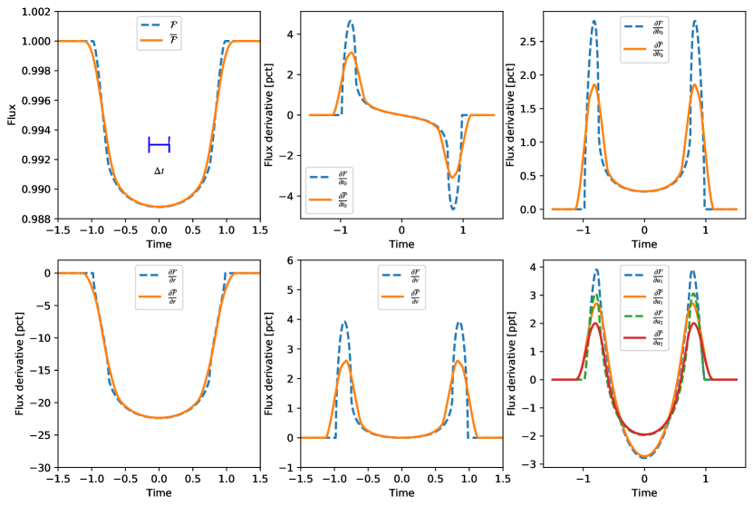
Figure 7: Comparison of the normalized flux and its derivatives with and without time-integration (see solid and dashed lines, respectively). The integration time, $\Delta t=0.3$, is indicated in the upper left panel with a horizontal blue line. The derivatives are computed with respect to $\{r,t_{0},v,b_{0},u_{1},u_{2}\}$. The parameters are given by $r=0.1$, $t_{0}=0$, $v=1$, $b_{0}=0.5$, and $u_{1}=u_{2}=0.3$.   

In practice the $\epsilon_{tol}$ parameter controls the average number of evaluations per exposure time, while the tolerance achieved is typically $<10\epsilon_{tol}$. Figure 8 shows the maximum numerical error achieved for computations with $\epsilon_{tol}=(10^{-4},10^{-6},10^{-8},10^{-10},10^{-12},10^{-14})$ relative to a precision of $\epsilon_{tol}=10^{-16}$. The computed model has $10^{4}$ exposures for quadratic limb-darkening with the same parameters as in Figure 7 (note that these exposures overlap in time; in practice many fewer exposures would be required to compute this light curve). In computing the time-integrated light curves, we integrate over the difference of the flux minus one, so that shallow transit depths will not lose precision. In Figure 8, the achieved precision is plotted versus the average number of evaluations per exposure for $\overline{F}(t)-1$ and for each of the derivatives. In all cases but the highest precision, the flux and all derivatives achieve a precision which is better than $10\epsilon_{tol}$. For the highest tolerance case, $\epsilon_{tol}=10^{-14}$, we find that the precision exceeds this value slightly; this is likely due to the model reaching the limit of double-precision.

Also plotted in Figure 8 is ten times the tolerance versus the evaluation time per exposure relative to the time for a single evaluation per exposure (dashed line). This curve falls to the right of the number ratio line (dotted line) by about a factor of $\sim 2$ for high tolerance ($\epsilon_{tol}=10^{-4}$), to about a factor of $1.3$ for low tolerance ($\epsilon_{tol}=10^{-14}$). Thus, the time per evaluation for the adaptive time-integrated flux and derivatives exceeds the expectation given a single evaluation per exposure. This is likely due to the fact that the model computation takes longer for some parameter values than others, while the adaptive integration tends to concentrate the evaluations at the parameters which are more expensive to evaluate. In addition there may be computation overhead from the adaptive Simpson integration function.

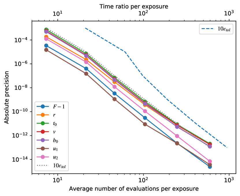
Figure 8: Precision achieved for the time-integrated flux (minus one) versus the average number of evaluations per exposure. The colored lines show the precision achieved for $\overline{F}(t)-1$ and for each of the derivatives. For comparison, the dotted line shows 10 times the tolerance, $\epsilon_{tol}$. The dashed line uses as the abscissa the ratio of the total light curve evaluation time per exposure relative to a single evaluation per exposure.   

8 Non-linear limb darkening

Claret (2000) introduced a “non-linear” limb darkening model which was found to be an effective model for describing the limb darkening functions which are produced by models of stellar atmospheres. Although we can only model limb darkening in integer powers of $\upmu$, we can use a high order polynomial model as an alternative limb darkening model.

We have computed an example non-linear light curve with $r=0.1$ and $c_{1}=c_{2}=c_{3}=c_{4}=0.2$, and then fit it with the polynomial limb-darkening model with increasing orders of the polynomial approximation. The non-linear light curve model we computed numerically as the analytic expressions in Mandel & Agol (2002) are in terms of hypergeometric functions which are expensive to evaluate. We numerically compute the non-linear light curve with a “layer-cake” model in which sums of layers of surface brightness with a grid of increasing radii are added together to approximate the lightcurve; this is the approach taken in the numerical model used to compute the non-linear limb darkening light curves in the code of Mandel & Agol (2002), and it is analogous to the approach taken by Kreidberg (2015) for computing models with arbitrary limb darkening profiles.

When fitting the non-linear lightcurve with the polynomial model, we find that the fit improves steadily up until $N=6$ (a sextic polynomial), while beyond sextic, the RMS improves imperceptibly. The RMS of the sextic fit for this example is $<5\times 10^{-7}$ relative to a depth of transit of about 1.4% (Figure 9).

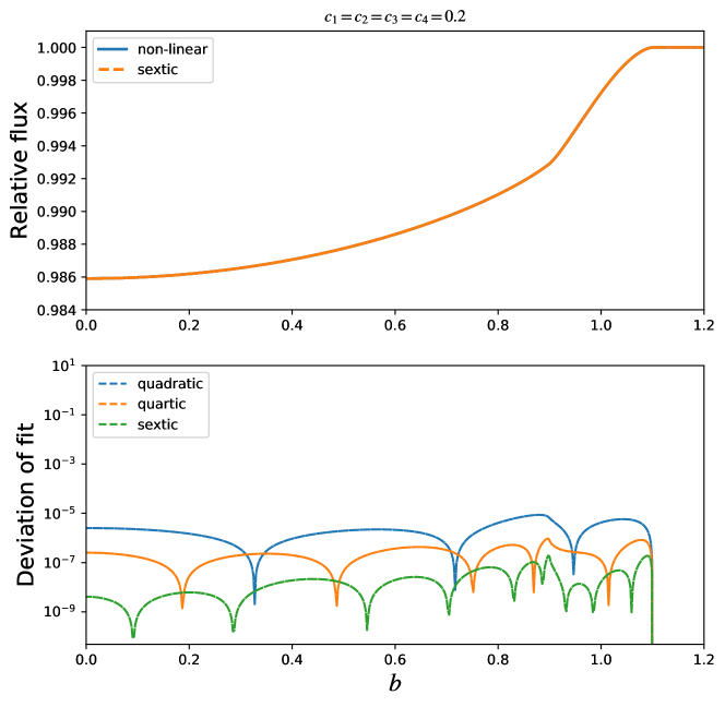
Figure 9: Comparison of the non-linear limb darkening with polynomial fits of various orders.   

This completes the description of the light curve computation, along with its derivatives. We now turn to discussing the implementation of the computation, followed by comparison with existing codes.

9 Implementation details

There are several details in our implementation of the foregoing equations which give further speedup of the computation, which we describe in this section.

When a light curve is computed, there are some computations which only need to be carried out once, and then can be reused at each time step in the light curve computation. We define a structure to hold these variables which are reused throughout the light curve; we also pre-allocate variables which are used throughout the computation to avoid the overhead of memory allocation and garbage collection. In addition, due to the greater computational expense of square-roots and divisions, where possible we try to only compute a square root or division once, storing these in a variable within the structure, and then reuse these with cheaper multiplication throughout the computation when needed. For instance, for many formulae we require the inverse of an integer, so an array of integer inverses is computed once and stored, and then accessed as required rather than recomputed.

Once the number of limb darkening terms, $N$, is specified, then the series coefficients for $\mathcal{M}_{n}$ and $\mathcal{N}_{n}$, $\alpha_{j}$ and $\gamma_{j}$, are a simple function of $j$ and $n$, and so we compute these coefficients once, and store them in a vector for $k^{2}\leq 1$, separately for $N-3$ to $N$ for $\mathcal{M}_{n}$, and for $N-1$ and $N$ for $\mathcal{N}_{n}$.

In addition, once $N$ is specified, then the transformation matrix for the Jacobian from $\mathfrak{g}_{i}$ to $u_{j}$, $\frac{\partial\mathfrak{g}_{i}}{\partial u_{j}}=\mathcal{A}$, remains the same throughout the light curve computation, so we compute this matrix only once, and then compute the flux derivative (Equation 98) with matrix multiplication. In fact, since the Jacobian matrix for transforming the derivatives from $\mathfrak{g}_{i}$ to $u_{j}$ can be expensive to apply, we can carry out the gradient of the likelihood function with respect to $\mathfrak{g}_{i}$, and then apply the Jacobian transformation from $\mathfrak{g}_{i}$ to $u_{j}$ only once to obtain the gradient of the likelihood with respect to the limb darkening parameterization. In practice, we are usually only concerned with optimizing a likelihood or computing gradients of a likelihood for Hamiltonian Markov Chain Monte Carlo, so the derivatives of the particular points in the light curve with respect to $u_{i}$ aren’t needed. This results in a significant computational savings, especially for large $N$. Transformation to other parameterizations, such as $q_{1}$ and $q_{2}$ defined by Kipping (2013) for quadratic limb-darkening, may also be accomplished after the fact by applying the Jacobian to compute the gradient of the likelihood in terms of these transformed parameters.

In computing the elliptic integrals, cel, we found that several terms which appear in the Bartky formalism are repeated amongst all three elliptic integrals which appear in the expressions for $\mathfrak{s}_{1}$. Consequently, we carry out a parallel computation of these elliptic integrals such that these repeated terms are only computed once; this improves the efficiency of the elliptic integral computations. Once these elliptic integrals are computed for $\mathfrak{s}_{1}$, the elliptic integrals $\mathrm{cel}(k_{c},1,1,k_{c}^{2})=E(m_{k})$ and $\mathrm{cel}(k_{c},1,1,0)=(E(m_{k})-(1-m_{k})K(m_{k}))/m_{k}$ are stored in the structure and reused for computing $\mathcal{M}_{n}$ and $\mathcal{N}_{n}$.

10 Benchmarking

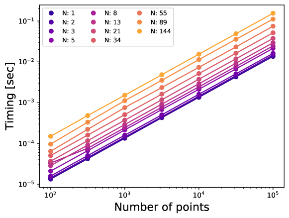
Figure 10: Scaling of the computation time in seconds with the number of data points in the light curve for $r=0.1$ with $b$ ranging from $0$ to $1.2$, and with the number of limb darkening coefficients, $N$.   

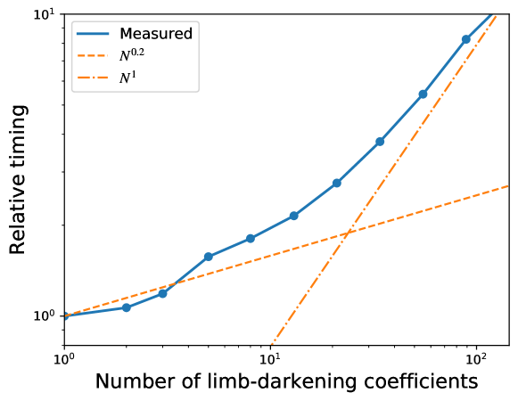
Figure 11: Scaling of the computation time with the number of limb darkening coeffients, $N$. The $y$-axis scales the timing with respect to the timing for a single limb darkening coefficient.   

We have measured the performance of the limb-darkened light curves with derivatives as a function of the number of computed data points and as a function of the number of limb darkening coefficients. We have computed the timing for $r=0.1$ and for a number of impact parameters ranging from $10^{2}$ to $10^{6}$, and the number of limb darkening coefficients ranging from $1$ to $144$. For each set of timing benchmark parameters, we carried out nine measurements of the timing, and we use the median of these for plotting purposes. The benchmarking for the Julia code was carried out with v0.7 of Julia on the trusty Ubuntu environment of Travis-CI on a 2.3 GHz 2-core machine with 7.5 GB of RAM. No time-integration/sub-sampling was carried out in this computation.

Figure 10 shows that the time dependence is linear with the number of $b$ values (which is equivalent to the number of data points in the light curve). The linear scaling with time holds for each value of the number of limb darkening coefficients.

Figure 11 shows that the time dependence scales approximately as $N^{0.2-1}$. As with the number of light-curve points, we have taken the median over nine measurements for each set of parameters. We then scaled the timing to the single-coefficient case, and took a second median over the number of light curve points.

10.1 Limitation of precision with order of limb-darkening

We find that the precision of the computation begins to degrade for $N\approx 25-30$. When computing limb-darkened light curves for very high order limb-darkening, we have found that the precision can be limited by cancellations which occur between different orders of the limb darkening. For standard polynomial limb-darkening, we find that the $\mathfrak{g}_{n}$ alternates between very large positive and negative values which can end up cancelling to produce a smaller amplitude light curve. These cancellations can lead to round-off and truncation errors which limit the precision of the computation.

Figure 12 shows the values of the $\mathfrak{g}_{n}$ coefficients for $u_{1}=u_{2}=...=u_{20}=0.05$ with $N=20$. Due to the alternating signs of coefficients in the binomial expansion, the $\mathfrak{g}_{n}$ values flip between large negative and large positive values, in this case varying in amplitude by about seven orders of magnitude from the smallest coefficient to the largest. Despite the large values of $\mathfrak{g}_{n}$, the light curve computed has a much smaller value with a depth of $\approx 1$% for a planet with a radius ratio of $r=0.1$ due to a fine-tuned cancellation between these large coefficients. This cancellation is precise for smaller values of $N$ and gradually increases with $N$.

Figure 13 shows the fractional error found by computing a light curve at double precision with a lightcurve computed at BigFloat versus the order of the limb darkening. Ten trials were made in which each of the limb-darkening coefficients was randomly chosen between zero and one, and the sum of their values was normalized to unity. In the figure the fractional error is computed relative to the transit depth for a planet-star radius ratio of $r=0.1$. For polynomial limb-darkening order of $N=30$ the fractional error can approach $10^{-6}$. Consequently we urge caution when using this model with large values of the polynomial order $N$; the light curve should be checked against a higher precision computation for some typical values of the parameters to gauge the accuracy of the model.

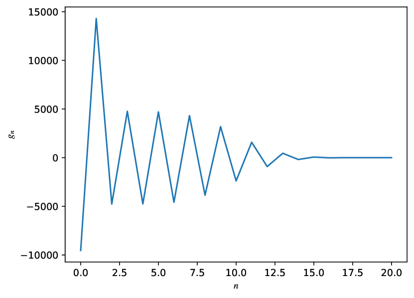
Figure 12: Values of the $\mathfrak{g}_{n}$ vector versus $n$ for $N=20$ and for uniform values of $u_{n}=1/20$.   

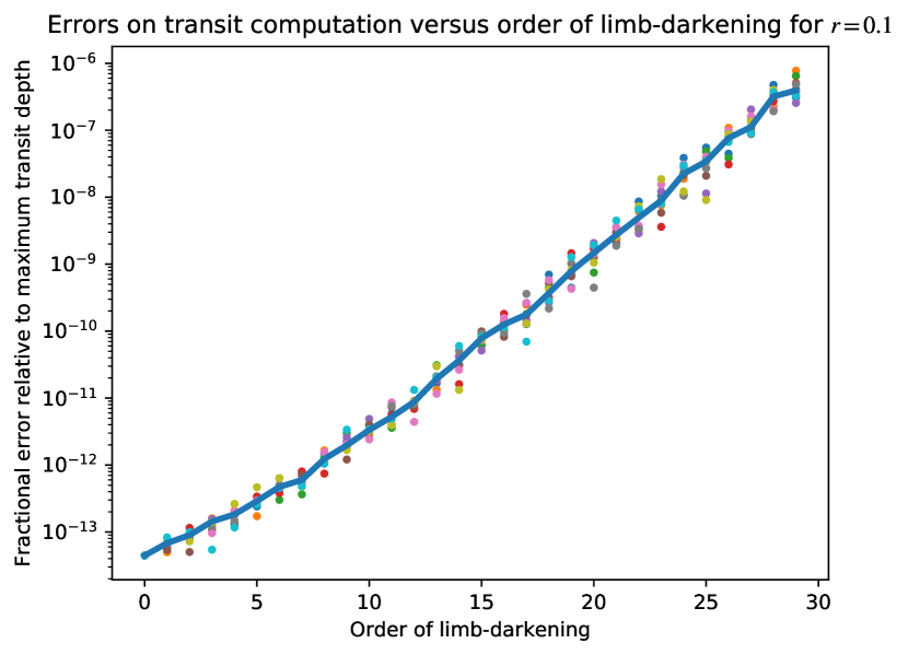
Figure 13: The fractional error on a light curve computed as a function of $N$, the order of the limb-darkening. The dotted points show the results of the maximum fractional error (relative to the depth of the transit) for ten different random realizations of the $u_{n}$ limb-darkening coefficients. The thick solid curve shows the median of these ten realizations.   

11 Comparison with prior work

In this section we compare our computations with existing code in terms of accuracy and speed. We compare both the Julia version of our code and an implementation of our algorithms in the starry package, with and without the computation of gradients. To ensure a fair comparison between the codes, we perform all calculations on a single core without multi-threading or interpolation over a pre-computed grid, which is an option in some codes.

11.1 Comparison with Mandel & Agol (2002)

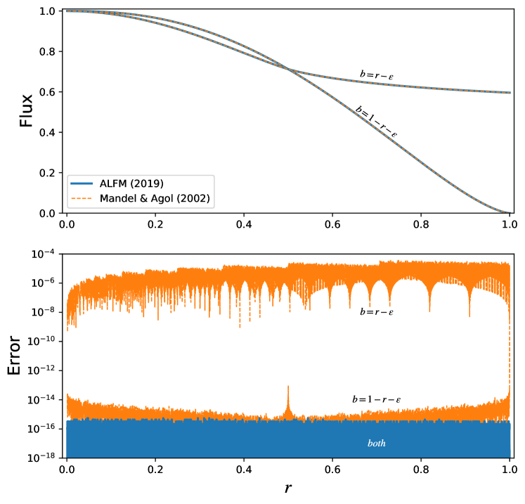
Figure 14: Comparison of Mandel & Agol (2002) with Agol, Luger, & Foreman-Mackey (2019).   

For uniform, linear or quadratic limb darkening, the IDL package EXOFAST improved upon the speed of the widely used computation by Mandel & Agol (2002) by utilizing the Bulirsch (1965a, b) expressions for the complete elliptic integral of the third kind which is needed for the linear case (Eastman et al., 2013). EXOFAST also uses a series approximation for the complete elliptic integrals of the first and second kind (Hastings, 1955). These three elliptic integrals, especially the third kind, are the bottleneck in the computation, and the Bulirsch version is faster than widely used Carlson implementation of elliptic integrals (Carlson, 1979).

We have carried out a numerical comparison of the EXOFAST implementation of the Mandel & Agol (2002) formulae for the linear case ($u_{1}=1$), and find that the most severe errors occur for $b=r\pm\epsilon$. Figure 14 shows the computed models and the errors as a function of $r$ for $b=1-r-\epsilon$ and $b=r-\epsilon$, with $\epsilon=10^{-12}$ (the results look very similar with $+\epsilon$, so we have only plotted one case for clarity). In the $b\approx 1-r$ case (near second and third contacts), the errors are larger than our new expression, reaching $\approx 10^{-10}$ for $r=1$. However, the errors become much more severe in the $b\approx r$ case. For $b=r\pm 10^{-12}$, the errors grow to $10^{-4}$, and continue to grow as $b$ gets closer to $r$. No such instability occurs for our new expressions, demonstrating their utility in all regions of parameter space.

A speed comparison for a transit computed with $10^{7}$ data points shows that the Julia implementation of these routines takes about 55% of the CPU time as the IDL EXOFAST implementation without derivatives, and about 65% of the computation time when including the derivatives. Consequently, we conclude that our new implementation is both faster (by 35-45%) and more accurate than the Mandel & Agol (2002) IDL implementation.

We note that EXOFAST v2.0 has now been updated to utilize the numerically-stable quadratic limb darkening expressions given above, albeit without the computed derivatives (Eastman et al., submitted).

11.2 Derivative comparison with Pál

We have computed the quadratic limb-darkened light curve using the F77 code written by András Pál, ntiq_fortran.f. Figure 15 shows the results of this comparison. The light curve models agree quite well, as do the derivatives, which is a good check on both codes. However, we find that the Pál model only achieves single precision for the computation, with errors reaching as much as a few $\times 10^{-8}$ for the flux and the derivatives with respect to the limb darkening parameters. One possible origin for this difference is that Pál (2008) uses the Carlson implementation of elliptic integrals (Carlson, 1979), which in this implementation may be be both less precise and slower to evaluate than our new implementation of the Bulirsch (1965a) code for computing elliptic integrals.

We have also compared the evaluation speed of our code with Pál’s. We compiled Pál’s code using gfortran -O3, and found that the computation of quadratic limb-darkened light curves and derivatives takes an average of 0.52 seconds to compute $10^{6}$ models, while the transit_poly_struct.jl takes an average of 0.16 seconds, giving our Julia code a 70% speed advantage over the Fortran code.

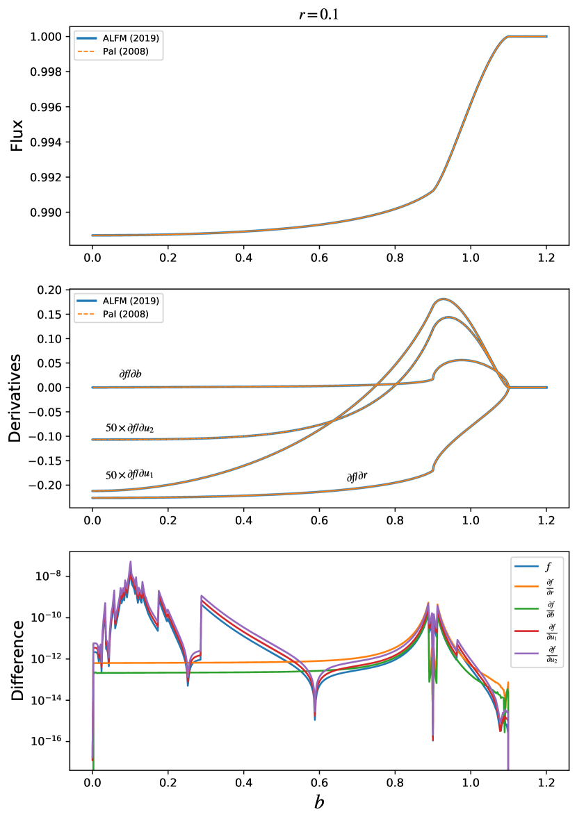
Figure 15: Comparison of Pál (2008) with Agol, Luger, & Foreman-Mackey (2019). The coefficients are $u_{1}=0.2$ and $u_{2}=0.3$.   

11.3 Comparison to batman

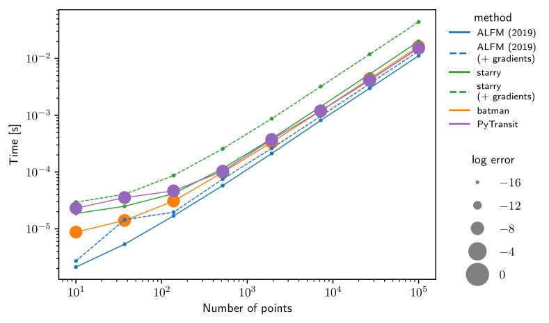
Figure 16: Comparison of Kreidberg (2015) (orange) with Agol, Luger, & Foreman-Mackey (2019) (Julia implementation in blue and starry implementation in green) for a transit across a quadratically limb-darkened star. Also shown are points corresponding to the computation using PyTransit (Parviainen, 2015). Dashed lines indicate computations including the gradients of the flux with respect to the radius, impact parameter, and all limb darkening coefficients. The $y$-axis corresponds to the evaluation time of the model in seconds and the size of the points is proportional to the log of the error in the computation relative to a calculation performed at 128-bit precision.   

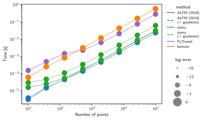
Figure 17: Similar to Figure 16, but this time comparing the computation of a transit across a nonlinearly limb-darkened star.   

A Python implementation of transit light curves which has been widely applied is the batman package (Kreidberg, 2015). This package implements a fast C version of the computation, called by Python for ease of use.

The batman package computes the quadratic limb darkening model of Mandel & Agol (2002), and uses the same approach for computing the complete elliptic integrals as EXOFAST. We have made a comparison of our implementation of quadratic limb darkening with batman, which is shown in Figure 16. Without computing derivatives, our approach (as implemented in Julia; blue) takes about 60% of the time of batman (orange); with derivatives, the two are comparable in speed. The implementation of our algorithm in starry (green) is similar in speed to batman without derivatives, and about a factor of 2 slower than batman when derivatives are computed. Both the Julia and starry implementations have errors close to double precision and are therefore many orders of magnitude more precise than batman.

Next, we ran a comparison with the non-linear limb darkening model which proves to be a better fit than the quadratic model to both simulated and observed stellar atmospheres. The batman code carries out a numerical integration over the surface brightness as a function of radius over the stellar disk, which requires additional computational time and limits the precision. We have carried out a fit to the non-linear limb darkening profile with $c_{1}=c_{2}=c_{3}=c_{4}=0.2$ with a polynomial limb darkening model with $N=15$ (§8). We then ran a timing comparison between the batman model and the polynomial model, and we find that the polynomial model is about 7 times more accurate and 25 times faster (Julia) and 20 times faster (starry) to evaluate compared with batman (Figure 17).

11.4 Comparison to PyTransit

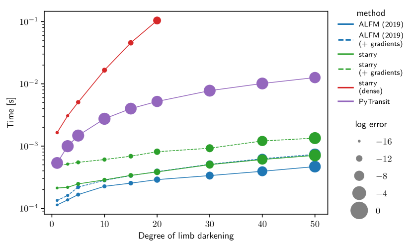
Figure 18: Comparison of the algorithm presented in this work (blue and green points) to that of Giménez (2006) for the computation of a transit across a star with polynomial limb darkening, as implemented in the PyTransit package (Parviainen, 2015) (purple points), as a function of the order of the polynomial. As before, the $y$-axis corresponds to the evaluation time and the size of the points to the log of the error in the computation. For reference, the red points correspond to the evaluation using a naive implementation of the full spherical harmonic formalism of Luger et al. (2019a), which this paper has improved upon.   

Another popular implementation of transit light curve computation is the PyTransit code (Parviainen, 2015). We have included points corresponding to this code in Figures 16 and 17, and in general find that it is comparable to batman in both evaluation time and accuracy. However, unlike batman, PyTransit implements the algorithm of Giménez (2006) for polynomial limb darkening (Equation 2).

In Figure 18 we therefore compare our implementation to the Giménez algorithm implementation in PyTransit as a function of the degree of limb darkening. We find our algorithm to be approximately between 5 (for low-order limb darkening) and 30 (for high-order limb darkening) times faster, and many orders of magnitude more precise for low order limb-darkening, while gradually degrading in precision to higher order limb-darkening to become comparable at very high orders ($N=50$). Even when computing derivatives, our Julia code is still faster by a about a factor of 2.5 for low-order limb-darkening, $N=0$, increasing in speed relative to the Giménez algorithm by about an order of magnitude at high-orders, $N=50$.

For reference, in Figure 18, we also plot the evaluation time when computing the light curve using the spherical harmonic formalism of Luger et al. (2019a). Because the algorithm presented in that paper computes surface integrals via recursions in both the spherical harmonic degree $l$ and the order $m$ (as it was designed to solve the occultation problem for arbitrary surface features), it scales super-quadratically with the degree of limb darkening. That algorithm is therefore orders of magnitude slower to evaluate in the case of pure limb darkening ($m=0$ modes only). We have modified the starry package to compute light curves using the formalism in this paper in the case of pure limb darkening.

12 Discussion

We have presented formulae for the transit (or occultation/eclipse) of a limb-darkened body with a limb darkening profile which is given by a polynomial in $\upmu$. These formulae have multiple assumptions built in: both bodies are treated as spherical (but see Seager & Hui, 2002; Hui & Seager, 2002), so that their projected sufaces are assumed to be circular (but see Barnes & Fortney, 2003, 2004; Barnes et al., 2009; Dobbs-Dixon et al., 2012); limb darkening is treated as azimuthally-symmetric (but see Barnes, 2009); refraction and any relativistic effects are ignored (but see Sidis & Sari, 2010); and the edges of both bodies are assumed to have a sharp boundary. All of these assumptions are violated in every transit event to some extent, but in the majority of cases these assumptions can yield a sufficiently precise model for a given signal-to-noise ratio.

Given these assumptions, generally one next assumes a particular functional form for the limb darkening law (Csizmadia, 2018). The parameterization of the limb darkening model can impact the precision of the computation of transit light curves. A common approach is to derive limb darkening coefficients for a particular limb darkening model from stellar atmosphere models, and to either fix these at the tabulated values given an observing band and an estimate of stellar parameters (Claret & Bloemen, 2011; Howarth, 2011), or at least to place a prior that the limb darkening parameters should nearly match these values. This approach can have several pitfalls: the limb darkening model may not be sufficiently precise, the stellar atmosphere model may not be accurate, and the stellar parameters may not be precise. In computing limb darkening from stellar atmosphere models, the spherical nature of limb darkening can affect the transit light curve (Neilson & Lester, 2013; Neilson et al., 2017), and thus the limb darkening coefficients must be fit with care (Claret, 2018). Even more importantly, full three dimensional stellar atmosphere models appear to give a more accurate description of stellar limb darkening by capturing the structure of the atmosphere under the influence of granulation (Hayek et al., 2012; Magic et al., 2015). However, any physical model for a stellar atmosphere has limitations in the fidelity at which it can model actual stellar atmospheres, and any modeler can only explore a finite set of parameters (effective temperature, metallicity, surface gravity, and magnetic field strength). In practice, then, it may be most robust simply to let the limb darkening parameters be free parameters, to let the limb darkening model be as flexible as possible, and to let the limb darkening model be fit along with the radius ratio and orbital parameters (Csizmadia et al., 2012; Espinoza & Jordán, 2015).

Even so, this approach still assumes azimuthal symmetry for the star, while any model for the surface brightness of a star can only be approximate: to some extent most stars are convective, rotationally-oblate, spotted, oscillating, flaring, etc. The model we have presented, then, will only resemble any given star to a precision which is limited by the lack of uniformity of the actual stellar surface. This begs the question of why a numerically precise model is required for modelling transit light curves. The answer is computational accuracy and stability: this more accurate model can be used over all of parameter space, without returning spurious results, and the high precision enables computation of derivatives which are beneficial when optimizing model parameters, computing the Fisher information matrix, or deriving parameter posteriors with MCMC.

Since we are limited in the knowledge of the properties of any given star, the discrepancies of an azimuthally-symmetric limb-darkened model can be treated as a source of noise. The deviation of the star from the model can be absorbed into noise models that account for outliers, account for correlations in the noise, or actually try to model the deviations of the star from azimuthal symmetry, such as induced by star spots (e.g. Sanchis-Ojeda & Winn, 2011).

One question is what order of the limb darkening model to choose to fit the data? Here we suggest several possibile solutions. The order of the limb darkening can be varied until the chi-square no longer improves (subject to a penalty for the greater freedom in the model, such as Bayesian Information Criterion). A high-order limb darkening model can be chosen, with the coefficients regularized to favor small values; should the data require a higher-order model, then the coefficients will increase to accommodate the data. The parameterization of the limb darkening with terms with $\mathfrak{g}_{n}((n+2)\upmu^{n}-\upmu^{n-2})$ for $2\leq n\leq N$ may be particularly convenient for this model in that these terms do not contribute to the total flux of the star. A third possibility is to fit stellar atmosphere models with the polynomial limb darkening model until a sufficient precision is reached given that warranted by the data, and then to place priors on the limb darkening parameters, informed by the stellar limb darkening models. A fourth approach might be to choose a parameterization with a small number of free parameters, such as the non-linear “power-2” law advocated by Maxted (2018), and fit this parameterized limb darkening model with a high-order polynomial for a given set. Then, only the non-linear parameters need to be varied, while the polynomial coefficients will be a simple function of these non-linear parameters. In this approach it should be straightforward to linearize the polynomial limb darkening model fitting, which ought to yield good computational efficiency. A limitation of our computational approach is that the precision begins to degrade significantly for $N\approx 25-30$; however, we anticipate that such a high order will rarely be required.

13 Applications

We envision that this code will be used for fits to higher precision transit data, such as gathered by the James Webb Space Telescope (JWST; Beichman et al., 2014), which require an improved model of stellar limb darkening. Here we discuss some potential avenues for application of this model.

The derivatives of the time-integrated light curves may be used to revisit the Fisher information analysis as carried out by Price & Rogers (2014), as originally investigated without time-integration by Carter et al. (2008). Accounting for correlated noise in this analysis will give more plausible estimates for the impact of stellar variability on the determination of transit transmission spectroscopy and transit-timing variations (Foreman-Mackey et al., 2017). This limit will be encountered as more precise measurements are made by gathering more photons during a transit. For example, for some targets, one can expect to obtain $\sim 10^{2}$ times as many photons with JWST as collected with Kepler. With such higher precision, as well as the wavelength-dependence afforded by several JWST observing modes, one can expect that high fidelity transit models will be required for making precise measurements of transit parameters.

The detection of transit-timing variations with low-amplitude sinusoidal variations can make use of the fact that small variations in transit time can be expanded as a Taylor series to linear order in time so that perturbations in the transit time are the sum of a periodic component and a constant times the derivative of the limb-darkened light curve (Ofir et al., 2018). This approach requires derivatives of the light curve with respect to time, for which the Mandel & Agol (2002) computation is too imprecise near the points of contact, $b\approx r$ and $b\approx 1-r$, within an impact parameter distance of $10^{-4}$, as shown by Ofir et al. (2018), who interpolated over these regions with polynomials. However, our new precise formulae, with derivatives, will be useful for the perturbative approach to the detection of transit timing variations, avoiding the numerical errors inherent in the Mandel & Agol (2002) model over a narrow range of parameter space.

14 Conclusions

We have presented an analytic model for the transits, occultations, and eclipses of limb-darkened bodies with a polynomial dependence of the limb darkening on the $z$ component of the stellar surface (or, alternatively, the cosine of the angle from the sub-stellar point, $\upmu$). The model is more precise and accurate than prior models that we have compared to, especially near special limits such as the points of contact and the coincidence of the edge of the occultor with the center of the source. The model also compares favorably in speed of evaluation, about a factor of three faster than the code of to Pál (2008), 5-30 faster than that of Gimenez, a factor of 2-25 faster than batman (depending on the order of the limb darkening), and 35-45% faster than EXOFAST.

We expect that this code may be used both as a workhorse model for general fitting of transit models, as well as a tool for more specialized applications, such as photodynamical modeling of interacting planets (Carter et al., 2012), triple stars (Carter et al., 2011), and transiting circumbinary planets (Doyle et al., 2011).

During the preparation of this paper, a related paper appeared on the mutual eclipse of multiple bodies (Short et al., 2018). Their approach is complementary to ours in that they utilize Green’s theorem to carry out a numerical quadrature for mulitiple limb darkening models using the approach of Pál (2012). Their approach does not yet include the computation of derivatives, but it does allows for a wider range of limb darkening models than polynomial, it allows for computation of the Rossiter-McLaughlin effect, and it carries out the computation for multiple overlapping bodies.

The code presented in this paper is open source and is implemented in three different ways: one of which is a part of the starry package, http://github.com/rodluger/starry/, written in a combination of C++ and Python, another of which is implemented as the default transit model in the Python-based exoplanet package, http://github.com/dfm/exoplanet/ (Foreman-Mackey et al., in preparation), and a new code written in Julia, http://github.com/rodluger/Limbdark.jl/. We have also implemented the quadratic limb-darkened flux model in IDL, without derivatives; this is also available within the GitHub repository. We welcome usage of these codes, and contributions to further develop and enhance their capabilities.

All figures in this paper were autogenerated on Travis-CI from the latest version of our repository. Clickable icons (  ) next to each figure link to the source code used to produce them, and icons (  ) next to the main equations link to derivations or numerical proofs. We encourage the community to adopt similar practices to bolster the accessibility, transparency, and reproducibility of research in the field.

Appendix A Errata for Mandel & Agol (2002)

Here are a list of errata for Mandel & Agol (2002):

1. In Equation (7), $\lambda_{3}$ and $\lambda_{4}$ should have $2k\rightarrow 2p$ in arguments of the elliptic integrals.

2. In Equation (7), $\lambda_{5}$ should have $-\frac{2}{3}\Theta(p-1/2)$ at the end.

3. For Case 11 in Table 1, $\eta^{d}$ should be 1/2, not 1, and $\lambda^{d}$ should be zero, not 1. This mistake affects the code, but it is never encountered for planets that transit main-sequence stars since $p<1$. This typo was discussed in Eastman et al. (2013).

4. The case $z=1-p$ is missing for $z<p$ (as pointed out by Pal 2008).

5. There is a $\pi$ missing in the denominator of the second term on the right hand side of Equation (8).

With the exception of 3, none of these errors affected the publicly available code.

Appendix B Derivatives of general complete elliptic integral

In this appendix, we give the derivatives of $cel$ with respect to the input parameters.

$$\frac{\partial\mathrm{cel}(k_{c},p,a,b)}{\partial k_{c}} = \frac{-k_{c}}{p-k_{c}^{2}}\left[\mathrm{cel}(k_{c},k_{c}^{2},a,b)-\mathrm{cel}(k_{c},p,a,b)\right],$$  (B1)

$$\frac{\partial\mathrm{cel}(k_{c},p,a,b)}{\partial p} = \frac{\mathrm{cel}(k_{c},p,0,\lambda)+(b-ap)\mathrm{cel}(k_{c},1,1-p,k_{c}^{2}-p)}{2p(1-p)(p-k_{c}^{2})},$$  (B2)

$$\lambda = k_{c}^{2}(b+ap-2bp)+p(3bp-ap^{2}-2b),$$  (B3)

$$\frac{\partial\mathrm{cel}(k_{c},p,a,b)}{\partial a} = \mathrm{cel}(k_{c},p,1,0),$$  (B4)

$$\frac{\partial\mathrm{cel}(k_{c},p,a,b)}{\partial b} = \mathrm{cel}(k_{c},p,0,1).$$  (B5)

Appendix C Listing of symbols and floating point precisions used in the paper and codebase

Table LABEL:tab:symbols gives a list of the notation used throughout the main paper. Table 2 lists the IEEE 754 interchange formats utilized in four versions of this code (Limbdark.jl and starry) written in Julia, IDL, Python and C++.

Table 1: Symbols used in this paper

Symbol	Definition	Reference
$a_{n}$	Giménez coefficients	Equation ((LABEL:gimenez))
$\mathcal{A}$	Change of basis matrix: $\mathbf{u}$ to Green’s polynomials	Equation ((LABEL:A))
$\mathcal{A}_{1}$	Change of basis matrix: $\mathbf{u}$ to polynomials	Equation ((LABEL:A1))
$\mathcal{A}_{2}$	Change of basis matrix: polynonials to Green’s polynomials	Equation ((LABEL:gbasis))
$A_{lens}$	Lens-shaped area of overlap of two circles	Equation ((LABEL:MAuniform))
$A_{kite}$	Kite-shaped area b/w center of circles and points of contact	Equation ((LABEL:Kite_area))
$b$	Impact parameter in units of occulted body’s radius
$b_{0}$	Minimum impact parameter in time-integrated model	§7
$b_{c}$	Cutoff for using alternative expression for $d\mathcal{P}/db$	§6.2
$c_{1}-c_{4}$	Non-linear limb darkening coefficients	§8
${\mathbf{D}}\,\wedge$	Exterior derivative	Equation ((LABEL:DGg))
$\mathrm{cel}(k_{c},p,a,b)$	General complete elliptic integral (Bulirsch, 1969)	Equation ((LABEL:cel))
$E(\scaleto{\cdot}{6pt})$	Complete elliptic integral of the second kind	Equation ((LABEL:elliptic))
$F$	Normalized flux seen by observer	Equation ((LABEL:occint))
$\overline{F}$	Time-averaged normalized flux	Equation ((LABEL:avg_flux))
${}_{2}F_{1}$	Generalized Hypergeometric function	Equation ((LABEL:Mn_series))
$\tilde{\mathfrak{g}}$	Green’s basis	Equation ((LABEL:greensbasis))
$\mathfrak{g}$	Vector in the basis $\tilde{\mathfrak{g}}$
${\mathbf{G}}_{n}$	Anti-exterior derivative of the $n^{\mathrm{th}}$ term in the Green’s basis	Equation ((LABEL:greens_n))
$i$	Dummy index
$I$	Specific intensity, $I(\mbox{$x$},\mbox{$y$})$
$I_{0}$	Intensity normalization constant	Equation ((LABEL:normalization))
$j$	Dummy index
$k$	Elliptic parameter	Equation ((LABEL:k2))
	Dummy index
$k_{c}$	$\sqrt{1-k^{2}}$	Equation ((LABEL:cel))
$K(\scaleto{\cdot}{6pt})$	Complete Elliptic integral of the first kind	Equation ((LABEL:elliptic))
$m_{k}$	Elliptic integral parameter	§4
$n$	Order of limb darkening/Green’s basis
$\mathcal{M}_{n}(r,b)$	Integral computed recursively	Equation ((LABEL:M_of_n))
$N$	Highest order of limb darkening polynomial
$\mathcal{N}_{n}(r,b)$	Integral computed recursively	Equation ((LABEL:N_of_n))
$p$	Cofficient of $cel$	Equation ((LABEL:cel))
$\tilde{\mathfrak{p}}$	Polynomial basis	Equation ((LABEL:polybasis))
$\mathfrak{p}$	Vector in the basis $\tilde{\mathfrak{p}}$
$q$	Term in cel identities	Equation ((LABEL:cel_identities))
	Term in cel $\Lambda$	Equation ((LABEL:biglam_stable))
$\mathcal{P}$	Primitive integral along perimiter of occultor	Equation ((LABEL:primitiveP))
$\mathcal{Q}$	Primitive integral along perimiter of occulted body	Equation ((LABEL:primitiveQ))
$r$	Occultor radius in units of occulted body’s radius	§1
${\mathbf{r}}$	Vector for integration over boundary of visible disk	Equation ((LABEL:greens))
$\mathfrak{s}$	Occultation light curve solution vector	Equation ((LABEL:greens))
$t$	Time variable	§7
$t_{0}$	Central time of transit	§7
$u_{1},u_{2}$	Quadratic limb darkening coefficients	Equation ((LABEL:quadraticld))
$\tilde{\mathbf{u}}$	Limb darkening basis	Equation ((LABEL:ldbasis))
${\mathbf{u}}$	Vector of limb darkening coefficients in the basis $\tilde{\mathbf{u}}$	§2
$v$	Velocity in time-integrated model	§7
${\mathbf{x}}$	Parameters used in time integration	§7
$x$	Cartesian coordinate	Equation ((LABEL:xyz))
$y$	Cartesian coordinate	Equation ((LABEL:xyz))
$z$	Cartesian coordinate, $z=\sqrt{1-\mbox{$x$}^{2}-\mbox{$y$}^{2}}$	Equation ((LABEL:xyz))
$\alpha_{j}$	Coefficient in series for $\mathcal{M}_{n}$	Equation ((LABEL:Mn_series))
$\gamma_{j}$	Coefficient in series for $\mathcal{N}_{n}$	Equation ((LABEL:Nn_series))
$\Gamma$	Gamma function
$\eta$	Parameter in quadratic limb darkening term	Equation ((LABEL:eta))
$\theta$	Polar angle on star with respect to observer
$\Theta$	Heaviside step function	Equation ((LABEL:biglam))
$\kappa_{0}$	Angular position of occultor/occulted intersection point	Equation ((LABEL:cosine_formulation))
$\kappa_{1}$	Angular position of occultor/occulted intersection point	Equation ((LABEL:cosine_formulation))
$\lambda$	Angular position of occultor/occulted intersection point	Equation ((LABEL:primitiveQdef))
	Term in cel identities	Equation ((LABEL:cel_identities))
$\Lambda^{e}$	Term in uniform transit expression	Equation ((LABEL:MAuniform))
$\Lambda$	Mandel & Agol (2002) function	Equation ((LABEL:biglam))
$\upmu$	Cosine of polar angle on star, $\upmu=z$	Equation ((LABEL:quadraticld))
$\Pi(\scaleto{\cdot}{6pt},\scaleto{\cdot}{6pt})$	Complete elliptic integral of the third kind	Equation ((LABEL:elliptic))
$\phi$	Angular position of occultor/occulted intersection point	Equation ((LABEL:primitivePdef))
$\varphi$	Dummy integration variable
$\xi$	Transformed integration variable	Equation ((LABEL:greens_transformed))

Table 2: Floating point standards used in implementations of code.

Language	Variable type	IEEE 754 interchange format	precision for 1.0
Julia	Float64	binary64	$2^{-52}=2.22\times 10^{-16}$
Julia	BigFloat	binary256	$2^{-255}=1.73\times 10^{-77}$
IDL	double	binary64	$2^{-52}=2.22\times 10^{-16}$
Python	double	binary64	$2^{-52}=2.22\times 10^{-16}$
C++	double	binary64	$2^{-52}=2.22\times 10^{-16}$

References

- Abramowitz & Stegun (1970) Abramowitz, M., & Stegun, I. A. 1970, Handbook of Mathematical Functions: With Formulas, Graphs, and Mathematical Tables (Washington, D.C.: U.S. Dept. of Commerce, National Bureau of Standards)
- Agol et al. (2005) Agol, E., et al. 2005, Monthly Notices of the Royal Astronomical Society, 359, 567. https://doi.org/10.1111/j.1365-2966.2005.08922.x
- Alonso (2018) Alonso, R. 2018, in Handbook of Exoplanets (Springer International Publishing), 1441–1467. https://doi.org/10.1007/978-3-319-55333-7_40
- Barnes (2009) Barnes, J. W. 2009, The Astrophysical Journal, 705, 683. https://doi.org/10.1088/0004-637x/705/1/683
- Barnes et al. (2009) Barnes, J. W., et al. 2009, The Astrophysical Journal, 706, 877. https://doi.org/10.1088/0004-637x/706/1/877
- Barnes & Fortney (2003) Barnes, J. W., & Fortney, J. J. 2003, The Astrophysical Journal, 588, 545. https://doi.org/10.1086/373893
- Barnes & Fortney (2004) —. 2004, The Astrophysical Journal, 616, 1193. https://doi.org/10.1086/425067
- Bartky (1938) Bartky, W. 1938, Reviews of Modern Physics, 10, 264. https://doi.org/10.1103/revmodphys.10.264
- Beichman et al. (2014) Beichman, C., et al. 2014, Publications of the Astronomical Society of the Pacific, 126, 1134. https://doi.org/10.1086/679566
- Betancourt (2017) Betancourt, M. 2017, arXiv preprint arXiv:1701.02434
- Brown (2001) Brown, T. M. 2001, The Astrophysical Journal, 553, 1006. https://doi.org/10.1086/320950
- Bulirsch (1965a) Bulirsch, R. 1965a, Numerische Mathematik, 7, 78. https://doi.org/10.1007/bf01397975
- Bulirsch (1965b) —. 1965b, Numerische Mathematik, 7, 353. https://doi.org/10.1007/bf01436529
- Bulirsch (1969) —. 1969, Numerische Mathematik, 13, 305. https://doi.org/10.1007/bf02165405
- Burrows (2014) Burrows, A. S. 2014, Nature, 513, 345. https://doi.org/10.1038/nature13782
- Carlson (1979) Carlson, B. C. 1979, Numerische Mathematik, 33, 1. https://doi.org/10.1007/bf01396491
- Carter et al. (2008) Carter, J. A., et al. 2008, The Astrophysical Journal, 689, 499. https://doi.org/10.1086/592321
- Carter et al. (2011) —. 2011, Science, 331, 562. https://doi.org/10.1126/science.1201274
- Carter et al. (2012) —. 2012, Science, 337, 556. https://doi.org/10.1126/science.1223269
- Charbonneau et al. (2007) Charbonneau, D., et al. 2007, Protostars and Planets V, 701
- Claret (2000) Claret, A. 2000, A&A, 363, 1081
- Claret (2018) —. 2018, ArXiv e-prints, arXiv:1804.10135
- Claret & Bloemen (2011) Claret, A., & Bloemen, S. 2011, Astronomy & Astrophysics, 529, A75. https://doi.org/10.1051/0004-6361/201116451
- Cowan & Fujii (2017) Cowan, N. B., & Fujii, Y. 2017, in Handbook of Exoplanets (Springer International Publishing), 1–16. https://doi.org/10.1007/978-3-319-30648-3_147-1
- Crossfield (2015) Crossfield, I. J. M. 2015, Publications of the Astronomical Society of the Pacific, 127, 941. https://doi.org/10.1086/683115
- Csizmadia (2018) Csizmadia, S. 2018, in Handbook of Exoplanets (Springer International Publishing), 1–15. https://doi.org/10.1007/978-3-319-30648-3_41-1
- Csizmadia et al. (2012) Csizmadia, S., et al. 2012, Astronomy & Astrophysics, 549, A9. https://doi.org/10.1051/0004-6361/201219888
- Dobbs-Dixon et al. (2012) Dobbs-Dixon, I., et al. 2012, The Astrophysical Journal, 751, 87. https://doi.org/10.1088/0004-637x/751/2/87
- Doyle et al. (2011) Doyle, L. R., et al. 2011, Science, 333, 1602. https://doi.org/10.1126/science.1210923
- Eastman et al. (2013) Eastman, J., et al. 2013, Publications of the Astronomical Society of the Pacific, 125, 83. https://doi.org/10.1086/669497
- Espinoza & Jordán (2015) Espinoza, N., & Jordán, A. 2015, Monthly Notices of the Royal Astronomical Society, 450, 1879. https://doi.org/10.1093/mnras/stv744
- Feroz & Hobson (2008) Feroz, F., & Hobson, M. P. 2008, Monthly Notices of the Royal Astronomical Society, 384, 449. https://doi.org/10.1111/j.1365-2966.2007.12353.x
- Ford (2005) Ford, E. B. 2005, The Astronomical Journal, 129, 1706. https://doi.org/10.1086/427962
- Ford (2006) —. 2006, The Astrophysical Journal, 642, 505. https://doi.org/10.1086/500802
- Foreman-Mackey et al. (2017) Foreman-Mackey, D., et al. 2017, The Astronomical Journal, 154, 220. https://doi.org/10.3847/1538-3881/aa9332
- Giménez (2006) Giménez, A. 2006, Astronomy & Astrophysics, 450, 1231. https://doi.org/10.1051/0004-6361:20054445
- Girolami & Calderhead (2011) Girolami, M., & Calderhead, B. 2011, Journal of the Royal Statistical Society: Series B (Statistical Methodology), 73, 123. https://doi.org/10.1111/j.1467-9868.2010.00765.x
- Goldberg (1991) Goldberg, D. 1991, ACM Computing Surveys, 23, 5. https://doi.org/10.1145/103162.103163
- Hastings (1955) Hastings, C. 1955, Approximations for digital computers,, Princeton, N.J.: Princeton University Press
- Haswell (2010) Haswell, C. A. 2010, Transiting Exoplanets
- Hayek et al. (2012) Hayek, W., et al. 2012, Astronomy & Astrophysics, 539, A102. https://doi.org/10.1051/0004-6361/201117868
- Heller (2019) Heller, R. 2019, Astronomy & Astrophysics, 623, A137. https://doi.org/10.1051/0004-6361/201834620
- Hestroffer (1997) Hestroffer, D. 1997, A&A, 327, 199
- Holman (2005) Holman, M. J. 2005, Science, 307, 1288. https://doi.org/10.1126/science.1107822
- Howarth (2011) Howarth, I. D. 2011, Monthly Notices of the Royal Astronomical Society, 413, 1515. https://doi.org/10.1111/j.1365-2966.2011.18122.x
- Hui & Seager (2002) Hui, L., & Seager, S. 2002, The Astrophysical Journal, 572, 540. https://doi.org/10.1086/340017
- Kahan (2000) Kahan, W. 2000, Technical report, University of California, Berkeley
- Kipping (2010) Kipping, D. M. 2010, Monthly Notices of the Royal Astronomical Society, 408, 1758. https://doi.org/10.1111/j.1365-2966.2010.17242.x
- Kipping (2013) —. 2013, Monthly Notices of the Royal Astronomical Society, 435, 2152. https://doi.org/10.1093/mnras/stt1435
- Kopal (1950) Kopal, Z. 1950, Harvard College Observatory Circular, 454, 1
- Kreidberg (2015) Kreidberg, L. 2015, PASP, 127, 1161
- Kuncir (1962) Kuncir, G. F. 1962, Communications of the ACM, 5, 347. https://doi.org/10.1145/367766.368179
- Lamarche & Leroy (1990) Lamarche, F., & Leroy, C. 1990, Computer Physics Communications, 59, 359. https://doi.org/10.1016/0010-4655(90)90184-3
- Luger et al. (2019a) Luger, R., et al. 2019a, AJ, 157, 64
- Luger et al. (2019b) —. 2019b, arXiv e-prints, arXiv:1903.12182
- Madhusudhan (2019) Madhusudhan, N. 2019, Annual Review of Astronomy and Astrophysics, 57, 617. https://doi.org/10.1146/annurev-astro-081817-051846
- Magic et al. (2015) Magic, Z., et al. 2015, Astronomy & Astrophysics, 573, A90
- Mandel & Agol (2002) Mandel, K., & Agol, E. 2002, ApJL, 580, L171
- Maxted (2018) Maxted, P. F. L. 2018, ArXiv e-prints, arXiv:1804.07943
- Morello et al. (2017) Morello, G., et al. 2017, The Astronomical Journal, 154, 111. https://doi.org/10.3847/1538-3881/aa8405
- Neal et al. (2011) Neal, R. M., et al. 2011, Handbook of markov chain monte carlo, 2, 2
- Neilson & Lester (2013) Neilson, H. R., & Lester, J. B. 2013, Astronomy & Astrophysics, 556, A86. https://doi.org/10.1051/0004-6361/201321888
- Neilson et al. (2017) Neilson, H. R., et al. 2017, The Astrophysical Journal, 845, 65. https://doi.org/10.3847/1538-4357/aa7edf
- Ofir et al. (2018) Ofir, A., et al. 2018, The Astrophysical Journal Supplement Series, 234, 9. https://doi.org/10.3847/1538-4365/aa9f2b
- Pál (2008) Pál, A. 2008, Monthly Notices of the Royal Astronomical Society, 390, 281. https://doi.org/10.1111/j.1365-2966.2008.13723.x
- Pál (2012) Pál, A. 2012, MNRAS, 420, 1630
- Parviainen (2015) Parviainen, H. 2015, Monthly Notices of the Royal Astronomical Society, 450, 3233. https://doi.org/10.1093/mnras/stv894
- Parviainen & Aigrain (2015) Parviainen, H., & Aigrain, S. 2015, Monthly Notices of the Royal Astronomical Society, 453, 3822. https://doi.org/10.1093/mnras/stv1857
- Price & Rogers (2014) Price, E. M., & Rogers, L. A. 2014, The Astrophysical Journal, 794, 92. https://doi.org/10.1088/0004-637x/794/1/92
- Russell & Shapley (1912a) Russell, H. N., & Shapley, H. 1912a, The Astrophysical Journal, 36, 239. https://doi.org/10.1086/141960
- Russell & Shapley (1912b) —. 1912b, The Astrophysical Journal, 36, 385. https://doi.org/10.1086/141972
- Sanchis-Ojeda & Winn (2011) Sanchis-Ojeda, R., & Winn, J. N. 2011, The Astrophysical Journal, 743, 61. https://doi.org/10.1088/0004-637x/743/1/61
- Seager & Deming (2010) Seager, S., & Deming, D. 2010, Annual Review of Astronomy and Astrophysics, 48, 631. https://doi.org/10.1146/annurev-astro-081309-130837
- Seager & Hui (2002) Seager, S., & Hui, L. 2002, The Astrophysical Journal, 574, 1004. https://doi.org/10.1086/340994
- Seager & Mallen-Ornelas (2003) Seager, S., & Mallen-Ornelas, G. 2003, The Astrophysical Journal, 585, 1038. https://doi.org/10.1086/346105
- Short et al. (2018) Short, D. R., et al. 2018, The Astronomical Journal, 156, 297. https://doi.org/10.3847/1538-3881/aae889
- Sidis & Sari (2010) Sidis, O., & Sari, R. 2010, The Astrophysical Journal, 720, 904. https://doi.org/10.1088/0004-637x/720/1/904
- Udry et al. (2007) Udry, S., et al. 2007, Protostars and Planets V, 685
- Vallisneri (2008) Vallisneri, M. 2008, Physical Review D, 77, doi:10.1103/physrevd.77.042001. https://doi.org/10.1103/physrevd.77.042001
- Weisstein (2018) Weisstein, E. W. 2018, “Circle-Circle Intersection." From MathWorld - A Wolfram Web Resource., http://mathworld.wolfram.com/Circle-CircleIntersection.html, , , accessed 2018-07-09
- Winn (2008) Winn, J. N. 2008, Proceedings of the International Astronomical Union, 4, 99. https://doi.org/10.1017/s174392130802629x
- Winn (2010) Winn, J. N. 2010, Exoplanet Transits and Occultations, ed. S. Seager (University of Arizona Press), 55–77