Remarks on the energy inequality of a global $L^{\infty}$ solution to the compressible Euler equations for the isentropic nozzle flow

Abstract.

We study the compressible Euler equations in the isentropic nozzle flow. The global existence of an $L^{\infty}$ solution has been proved in (Tsuge in Nonlinear Anal. Real World Appl. 209: 217-238 (2017)) for large data and general nozzle. However, unfortunately, this solution does not possess finiteness of energy. Although the modified Godunov scheme is introduced in this paper, we cannot deduce the energy inequality for the approximate solutions.

Therefore, our aim in the present paper is to derive the energy inequality for an $L^{\infty}$ solution. To do this, we introduce the modified Lax Friedrichs scheme, which has a recurrence formula consisting of discretized approximate solutions. We shall first deduce from the formula the energy inequality. Next, applying the compensated compactness method, the approximate solution converges to a weak solution. The energy inequality also holds for the solution as the limit. As a result, since our solutions are $L^{\infty}$, they possess finite energy and propagation, which are essential to physics.

1. Introduction

The present paper is concerned with isentropic gas flow in a nozzle. This motion is governed by the following compressible Euler equations:

$$\left\{\begin{array}[]{ll}\displaystyle{\rho_{t}+m_{x}=a(x)m,}\\ \displaystyle{m_{t}+\left(\frac{m^{2}}{\rho}+p(\rho)\right)_{x}=a(x)\frac{m^{2}}{\rho},\quad x\in{\bf R}},\end{array}\right.$$ (1.1)

where $\rho$, $m$ and $p$ are the density, the momentum and the pressure of the gas, respectively. If $\rho>0$, $v=m/\rho$ represents the velocity of the gas. For a barotropic gas, $p(\rho)=\rho^{\gamma}/\gamma$, where $\gamma\in(1,5/3]$ is the adiabatic exponent for usual gases. The given function $a(x)$ is represented by

$$a(x)=-A^{\prime}(x)/A(x)\quad\text{with}\quad A(x)=e^{-\int^{x}a(y)dy},$$

where $A\in C^{2}({\bf R})$ is a slowly variable cross section area at $x$ in the nozzle.

We consider the Cauchy problem (1.1) with the initial data

$$(\rho,m)|_{t=0}=(\rho_{0}(x),m_{0}(x)).$$ (1.2)

The above problem (1.1)–(1.2) can be written in the following form

$$\left\{\begin{array}[]{lll}u_{t}+f(u)_{x}=g(x,u),\quad{x}\in{\bf R},\\ u|_{t=0}=u_{0}(x),\end{array}\right.$$ (1.5)

by using $u={}^{t}(\rho,m)$, $\displaystyle f(u)={}^{t}\!\left(m,\frac{m^{2}}{\rho}+p(\rho)\right)$ and $\displaystyle{g(x,u)={}^{t}\!\left(a(x)m,a(x)\frac{m^{2}}{\rho}\right)}$. The nozzle flow is applied in the various area, engineering, physics. Moreover, it is known that it is closely related to the flow of the solar wind. The detail can be found in [T7].

In the present paper, we consider an unsteady isentropic gas flow in particular. Let us survey the related mathematical results for the nozzle flow. The pioneer work in this direction is Liu [L1]. In [L1], Liu proved the existence of global solutions coupled with steady states, by the Glimm scheme, provided that the initial data have small total variation and are away from the sonic state. Recently, the existence theorems that include the transonic state have been obtained. The author [T1] proved the global existence of solutions for the spherically symmetric case ($A(x)=x^{2}$ in (1.1)) by the compensated compactness framework. Lu [L2], Gu and Lu [LG] extended [T1] to the nozzle flow with a monotone cross section area and the general pressure by using the vanishing viscosity method. In addition, the author [T4] treated the Laval nozzle, which is a divergent and convergent nozzle. In these papers, the monotonicity of the cross section area plays an important role. For the general nozzle, the author [T4] and [T5] proved the global existence of a solution, provided that $a\in L^{1}({\bf R})$.

However, unfortunately, these solutions [T1], [T4], [T5] and [T6] do not possess finiteness of energy. Although the modified Godunov scheme is introduced in these paper, we cannot deduce the energy inequality for the corresponding approximate solution. Since our solutions are weak ones, which are defined almost everywhere, it is difficult to deduce the energy inequality for the weak solutions directly. Our main purpose of the present paper is to prove the inequality for solutions. Our strategy is as follows. We introduce the modified Lax Friedrichs scheme. By using the scheme, we can obtain the global existence of a solution in a similar manner to the modified Godunov scheme. Moreover, this has a recurrence formula consisting of discretized approximate solutions (see (4.1)). We shall first deduce from the formula the energy inequality. Since it consists of discretized values such as sequence, the treatment is comparetively easy. Next, applying the compensated compactness, the approximate solutions converge to a weak solution. As a result, the energy inequality also holds for the weak solution as the limit. This idea is employed in [T2] and [T3]. In this paper, we prove the energy inequality for [T6] in particular. However, we can similarly apply our method to the other cases [T1], [T4] and [T5].

The above finite energy solutions have recently received attention in [CS] and [LW]. In these results, solutions are constructed in $L^{p}$. On the other hand, our solution is $L^{\infty}$, which yields finite propagation. Therefore, our solution possesses finiteness of both energy and propagation, which are essential to physics.

To state our main theorem, we define the Riemann invariants $w,z$, which play important roles in this paper, as

Definition 1.1.

$$w:=\frac{m}{\rho}+\frac{\rho^{\theta}}{\theta}=v+\frac{\rho^{\theta}}{\theta},\quad{z}:=\frac{m}{\rho}-\frac{\rho^{\theta}}{\theta}=v-\frac{\rho^{\theta}}{\theta}\quad(\theta:=(\gamma-1)/2).$$

These Riemann invariants satisfy the following.

Remark 1.1.

$$|w|\geq|z|,\;w\geq 0,\;\mbox{\rm when}\;v\geq 0.\quad|w|\leq|z|,\;z\leq 0,\;\mbox{\rm when}\;v\leq 0.$$ (1.6)

$$v=\frac{w+z}{2},\;\rho=\left(\frac{\theta(w-z)}{2}\right)^{1/\theta},\;m=\rho v.$$ (1.7)

From the above, the lower bound of $z$ and the upper bound of $w$ yield the bound of $\rho$ and $|v|$.

Moreover, we define the entropy weak solution.

Definition 1.2.

A measurable function $u(x,t)$ is called a global entropy weak solution of the Cauchy problems (1.5) if

$$\int^{\infty}_{-\infty}\int^{\infty}_{0}u\phi_{t}+f(u)\phi_{x}+g(x,u)\phi dxdt+\int^{\infty}_{-\infty}u_{0}(x)\phi(x,0)dx=0$$

holds for any test function $\phi\in C^{1}_{0}({\bf R}\times{\bf R}_{+})$ and

$$\int^{\infty}_{-\infty}\int^{\infty}_{0}\eta(u)\psi_{t}+q(u)\psi_{x}+\nabla\eta(u)g(x,u)\psi dxdt+\int^{\infty}_{-\infty}\eta(u_{0}(x))\psi(x,0)dx\geq 0$$ (1.8)

holds for any non-negative test function $\psi\in C^{1}_{0}({\bf R}\times{\bf R}_{+})$, where $(\eta,q)$ is a pair of convex entropy–entropy flux of (1.1) (see Section 2).

We assume the following.
There exists a nonnegative function $b\in C^{1}({\bf R})$ such that

$$\begin{split}|a(x)|\leq\mu b(x),\quad\max\left\{\int^{\infty}_{0}b(x)dx,\;\int^{0}_{-\infty}b(x)dx\right\}\leq\frac{1}{2}\log\frac{1}{\sigma},\end{split}$$ (1.9)

where $\mu=\frac{(1-\theta)^{2}}{\theta(1+\theta-2\sqrt{\theta})},\;\sigma=\frac{1-\theta}{(1-\sqrt{\theta})(2\sqrt{\theta+1}+\sqrt{\theta}-1)}$. Here we notice that $0<\sigma<1$.

From the similar argument of [T6], we have

Theorem 1.1.

We assume that, for $b$ in (1.9) and any fixed nonnegative constant $M$, initial density and momentum data $u_{0}=({\rho}_{0},{m}_{0})\in{L}^{\infty}({\bf R})$ satisfy

$$0\leq\rho_{0}(x),\;\;-Me^{-\int^{x}_{0}b(y)dy}\leq{z}(u_{0}(x)),\;\;w(u_{0}(x))\leq Me^{\int^{x}_{0}b(y)dy}\quad\text{\rm a.\,e. }x\in{\bf R}.$$ (1.10)

Then the Cauchy problem $(\ref{eqn:IP})$ has a global entropy weak solution $u(x,t)$ satisfying the same inequalities as (1.10)

$$0\leq\rho(x,t),\;\;-Me^{-\int^{x}_{0}b(y)dy}\leq{z}(u(x,t)),\;\;w(u(x,t))\leq Me^{\int^{x}_{0}b(y)dy}$$

$$\text{\rm a.\,e. }(x,t)\in{\bf R}\times{\bf R}_{+}.$$

Remark 1.2.

In view of $\eqref{eqn:condition-M}_{2}$, (1.10) implies that we can supply arbitrary $L^{\infty}$ data.

Then, our main theorem is as follows.

Theorem 1.2.

If the energy of initial data $\int_{\bf R}A(x)\eta_{*}(u_{0}(x))dx$ is finite, for the solution of Theorem 1.1, the following energy inequality holds.

$$\int_{\bf R}A(x)\eta_{*}(u(x,t))dx\leq\int_{\bf R}A(x)\eta_{*}(u_{0}(x))dx\quad\text{\rm a.\,e. }t>0,$$ (1.11)

where $\eta^{*}$ is the mechanical energy defined as follows.

$$\eta_{*}:=\frac{1}{2}\frac{m^{2}}{\rho}+\frac{1}{\gamma(\gamma-1)}\rho^{\gamma}$$

The present paper is organized as follows. In Section 2, we review the Riemann problem and the properties of Riemann solutions. In Section 3, we construct approximate solutions by the modified Lax Friedrichs scheme. In Section 4, we drive the recurrence formula consisting of discretized approximate solutions. We shall deduce the energy inequality for the formula.

2. Preliminary

In this section, we first review some results of the Riemann solutions for the homogeneous system of gas dynamics. Consider the homogeneous system

$$\left\{\begin{array}[]{ll}\rho_{t}+m_{x}=0,\\ \displaystyle{m_{t}+\left(\frac{m^{2}}{\rho}+p(\rho)\right)_{x}=0,\quad{p}(\rho)=\rho^{\gamma}/\gamma.}\end{array}\right.$$ (2.1)

A pair of functions $(\eta,q):{\bf R}^{2}\rightarrow{\bf R}^{2}$ is called an entropy–entropy flux pair if it satisfies an identity

$$\nabla{q}=\nabla\eta\nabla{f}.$$ (2.2)

Furthermore, if, for any fixed ${m}/{\rho}\in(-\infty,\infty)$, $\eta$ vanishes on the vacuum $\rho=0$, then $\eta$ is called a weak entropy. For example, the mechanical energy–energy flux pair

$$\eta_{*}:=\frac{1}{2}\frac{m^{2}}{\rho}+\frac{1}{\gamma(\gamma-1)}\rho^{\gamma},\quad q_{*}:=m\left(\frac{1}{2}\frac{m^{2}}{\rho^{2}}+\frac{\rho^{\gamma-1}}{\gamma-1}\right)$$ (2.3)

should be a strictly convex weak entropy–entropy flux pair.

The jump discontinuity in a weak solutions to (2.1) must satisfy the following Rankine–Hugoniot condition

$$\lambda(u-u_{0})=f(u)-f(u_{0}),$$ (2.4)

where $\lambda$ is the propagation speed of the discontinuity, $u_{0}=(\rho_{0},m_{0})$ and $u=(\rho,m)$ are the corresponding left and right state, respectively. A jump discontinuity is called a shock if it satisfies the entropy condition

$$\lambda(\eta(u)-\eta(u_{0}))-(q(u)-q(u_{0}))\geq 0$$ (2.5)

for any convex entropy pair $(\eta,q)$.

There are two distinct types of rarefaction and shock curves in the isentropic gases. Given a left state $(\rho_{0},m_{0})$ or $(\rho_{0},v_{0})$, the possible states $(\rho,m)$ or $(\rho,v)$ that can be connected to $(\rho_{0},m_{0})$ or $(\rho_{0},v_{0})$ on the right by a rarefaction or a shock curve form a 1-rarefaction wave curve $R_{1}(u_{0})$, a 2-rarefaction wave curve $R_{2}(u_{0})$, a 1-shock curve $S_{1}(u_{0})$ and a 2-shock curve $S_{2}(u_{0})$:

$$R_{1}(u_{0}):w=w_{0},\;\rho<\rho_{0},\quad R_{2}(u_{0}):z=z_{0},\;\rho>\rho_{0},$$

$$S_{1}(u_{0}):\displaystyle{v-v_{0}=-\sqrt{\frac{1}{\rho\rho_{0}}\frac{p(\rho)-p(\rho_{0})}{\rho-\rho_{0}}}(\rho-\rho_{0})\quad\rho>\rho_{0}>0,}$$

$$S_{2}(u_{0}):\displaystyle{v-v_{0}=\sqrt{\frac{1}{\rho\rho_{0}}\frac{p(\rho)-p(\rho_{0})}{\rho-\rho_{0}}}(\rho-\rho_{0})\quad\rho<\rho_{0},}$$

respectively. Here we notice that shock wave curves are deduced from theRankine–Hugoniot condition (2.4).

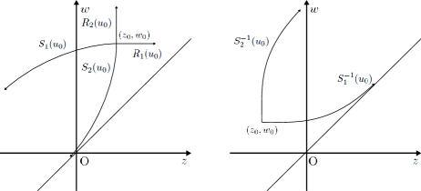
Figure 1. The rarefaction curves, the shock curves and the inverse rarefaction curves in $(z,w)$-plane

2.1. Riemann Solution

Given a right state $(\rho_{0},m_{0})$ or $(\rho_{0},v_{0})$, the possible states $(\rho,m)$ or $(\rho,v)$ that can be connected to $(\rho_{0},m_{0})$ or $(\rho_{0},v_{0})$ on the left by a shock curve constitute 1-inverse shock curve $S_{1}^{-1}(u_{0})$ and 2-inverse shock curve

$$S_{1}^{-1}(u_{0}):\displaystyle{v-v_{0}=-\sqrt{\frac{1}{\rho\rho_{0}}\frac{p(\rho)-p(\rho_{0})}{\rho-\rho_{0}}}(\rho-\rho_{0}),\quad\underline{\rho<\rho_{0}},}$$

$$S_{2}^{-1}(u_{0}):\displaystyle{v-v_{0}=\sqrt{\frac{1}{\rho\rho_{0}}\frac{p(\rho)-p(\rho_{0})}{\rho-\rho_{0}}}(\rho-\rho_{0}),\quad\underline{\rho>\rho_{0}>0},}$$

respectively.

Next we define a rarefaction shock. Given $u_{0},u$ on $S_{i}^{-1}(u_{0})\;(i=1,2)$, we call the piecewise constant solution to (2.1), which consists of the left and right states $u_{0},u$ a rarefaction shock. Here, notice the following: although the inverse shock curve has the same form as the shock curve, the underline expression in $S_{i}^{-1}(u_{0})$ is different from the corresponding part in $S_{i}(u_{0})$. Therefore the rarefaction shock does not satisfy the entropy condition.

We shall use a rarefaction shock in approximating a rarefaction wave. In particular, when we consider a rarefaction shock, we call the inverse shock curve connecting $u_{0}$ and $u$ a rarefaction shock curve.

From the properties of these curves in phase plane $(z,w)$, we can construct a unique solution for the Riemann problem

$$u|_{t=0}=\left\{\begin{array}[]{ll}u_{-},\quad{x}<x_{0},\\ u_{+},\quad{x}>x_{0},\end{array}\right.$$ (2.6)

where $x_{0}\in(-\infty,\infty)$, $\rho_{\pm}\geq 0$ and $m_{\pm}$ are constants satisfying $|m_{\pm}|\leq{C}\rho_{\pm}$. The Riemann solution consists of the following (see Fig. 2).

1. $(z_{+},w_{+})\in$ (I): 1-rarefaction curve and 2-rarefaction curve;

2. $(z_{+},w_{+})\in$ (II): 1-shock curve and 2-rarefaction curve;

3. $(z_{+},w_{+})\in$ (III): 1-shock curve and 2-shock curve;

4. $(z_{+},w_{+})\in$ (IV): 1-rarefaction curve and 2-shock curve,

where $z_{\pm}=m_{\pm}/\rho_{\pm}-(\rho_{\pm})^{\theta}/\theta,\;w_{\pm}=m_{\pm}/\rho_{\pm}+(\rho_{\pm})^{\theta}/\theta$ respectively.

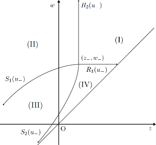
Figure 2. The elementary wave curves in $(z,w)$-plane

We denote the solution the Riemann solution $(u_{-},u_{+})$.

3. Construction of Approximate Solutions

In this section, we construct approximate solutions. In the strip $0\leq{t}\leq{T}$ for any fixed $T\in(0,\infty)$, we denote these approximate solutions by $u^{\varDelta}(x,t)=(\rho^{\varDelta}(x,t),m^{\varDelta}(x,t))$. Let ${\varDelta}x$ and ${\varDelta}{t}$ be the space and time mesh lengths, respectively. Moreover, for any fixed positive value $X$, we assume that

$$A(x)\text{ is a constant in }|x|>X.$$ (3.1)

Then we notice that $a(x)$ is bounded and has a compact support.

Let us define the approximate solutions by using the modified Lax Friedrichs scheme. We set

$$(j,n)\in\mbox{\bf Z}\times\mbox{\bf Z}_{\geq 0}.$$

In addition, using $M$ in (1.10), we take ${\varDelta}x$ and ${\varDelta}{t}$ such that

$$\frac{{\varDelta}x}{{\varDelta}{t}}=2Me^{\max\left\{\int^{\infty}_{0}b(x)dx,\;\int^{0}_{-\infty}b(x)dx\right\}}.$$

First we define $u^{\varDelta}(x,-0)$ by

$$u^{\varDelta}(x,-0)=u_{0}(x)$$

$$u^{\varDelta}(x,-0)=\chi_{\scriptscriptstyle{X}}(x)u_{0}(x),$$

where

$$\begin{split}\chi_{\scriptscriptstyle{X}}(x)=\left\{\begin{array}[]{ll}1,\quad x\leq X,\\ 0,\quad x\geq X\end{array}\right.\end{split}$$ (3.2)

and set

$$J_{n}=\{k;k+n=\text{even}\}.$$

Then, for $j\in J_{0}$, we define $E_{j}^{0}(u)$ by

$$E_{j}^{0}(u)=\frac{1}{2{\varDelta}x}\int_{{(j-1)}{\varDelta}x}^{(j+1){\varDelta}x}u^{\varDelta}(x,-0)dx.$$

Next, assume that $u^{\varDelta}(x,t)$ is defined for $t<n{\varDelta}{t}$. Then, for $j\in J_{n}$, we define $E^{n}_{j}(u)$ by

$$E^{n}_{j}(u)=\frac{1}{2{\varDelta}x}\int_{{(j-1)}{\varDelta}x}^{(j+1){\varDelta}x}u^{\varDelta}(x,n{\varDelta}{t}-0)dx.$$

Moreover, for $j\in J_{n}$, we define $u_{j}^{n}=(\rho_{j}^{n},m_{j}^{n})$ as follows.
We choose $\delta$ such that $1<\delta<1/(2\theta)$. If

$$E^{n}_{j}(\rho):=\frac{1}{2{\varDelta}x}\int_{{(j-1)}{\varDelta}x}^{(j+1){\varDelta}x}\rho^{\varDelta}(x,n{\varDelta}{t}-0)dx<({\varDelta}x)^{\delta},$$

we define $u_{j}^{n}$ by $u_{j}^{n}=(0,0)$; otherwise, setting

$$\begin{split}{z}_{j}^{n}:&=\max\left\{z(E_{j}^{n}(u)),\;-Me^{-\int^{j{\varDelta}x}_{0}b(x)dx}\right\}\\ &\hskip 100.0pt\mbox{and}\\ w_{j}^{n}:&=\min\left\{w(E_{j}^{n}(u)),\;Me^{\int^{j{\varDelta}x}_{0}b(x)dx}\right\},\end{split}$$ (3.3)

we define $u_{j}^{n}$ by

$$u_{j}^{n}:=(\rho_{j}^{n},m_{j}^{n}):=\left(\left\{\frac{\theta(w_{j}^{n}-z_{j}^{n})}{2}\right\}^{1/\theta},\left\{\frac{\theta(w_{j}^{n}-z_{j}^{n})}{2}\right\}^{1/\theta}\frac{w_{j}^{n}+z_{j}^{n}}{2}\right).$$

3.1. Construction of Approximate Solutions in the Cell

By using $u_{j}^{n}$ defined above, we construct the approximate solutions with $u^{\varDelta}((j-1){\varDelta}x,n{\varDelta}t+0)=u_{j-1}^{n}$ and $u^{\varDelta}((j+1){\varDelta}x,n{\varDelta}t+0)=u_{j+1}^{n}$in the cell $(j-1){\varDelta}x\leq{x}<(j+1){\varDelta}x,\;n{\varDelta}{t}\leq{t}<(n+1){\varDelta}{t}\quad(j\in J_{n+1},\;n\in{\bf Z}_{\geq 0})$.

We first solve a Riemann problem with initial data $(u_{j-1}^{n},u_{j+1}^{n})$. Call constants $u_{\rm L}(=u_{j-1}^{n}),u_{\rm M},u_{\rm R}(=u_{j+1}^{n})$ the left, middle and right states, respectively. Then the following four cases occur.

• Case 1 A 1-rarefaction wave and a 2-shock arise.

• Case 2 A 1-shock and a 2-rarefaction wave arise.

• Case 3 A 1-rarefaction wave and a 2-rarefaction arise.

• Case 4 A 1-shock and a 2-shock arise.

We then construct approximate solutions $u^{\varDelta}(x,t)$ by perturbing the above Riemann solutions. We consider only the case in which $u_{\rm M}$ is away from the vacuum. The other case (i.e., the case where $u_{\rm M}$ is near the vacuum) is a little technical. Therefore, we postpone the case near the vacuum to Appendix A.

The case where $u_{\rm M}$ is away from the vacuum

Let $\alpha$ be a constant satisfying $1/2<\alpha<1$. Then we can choose a positive value $\beta$ small enough such that $\beta<\alpha$, $1/2+\beta/2<\alpha<1-2\beta$, $\beta<2/(\gamma+5)$ and $(9-3\gamma)\beta/2<\alpha$.

We first consider the case where $\rho_{\rm M}>({\varDelta}x)^{\beta}$, which means $u_{\rm M}$ is away from the vacuum. In this step, we consider Case 1 in particular. The constructions of Cases 2–4 are similar to that of Case 1.

Consider the case where a 1-rarefaction wave and a 2-shock arise as a Riemann solution with initial data $(u_{j-1}^{n},u_{j+1}^{n})$. Assume that $u_{\rm L},u_{\rm M}$ and $u_{\rm M},u_{\rm R}$ are connected by a 1-rarefaction and a 2-shock curve, respectively.

Step 1.
In order to approximate a 1-rarefaction wave by a piecewise constant rarefaction fan, we introduce the integer

$$p:=\max\left\{[[(z_{\rm M}-z_{\rm L})/({\varDelta}x)^{\alpha}]]+1,2\right\},$$

where $z_{\rm L}=z(u_{\rm L}),z_{\rm M}=z(u_{\rm M})$ and $[[x]]$ is the greatest integer not greater than $x$. Notice that

$$p=O(({\varDelta}x)^{-\alpha}).$$ (3.4)

Define

$$z_{1}^{*}:=z_{\rm L},\;z_{p}^{*}:=z_{\rm M},\;w_{i}^{*}:=w_{\rm L}\;(i=1,\ldots,p),$$

and

$$z_{i}^{*}:=z_{\rm L}+(i-1)({\varDelta}x)^{\alpha}\;(i=1,\ldots,p-1).$$

We next introduce the rays $x=j{\varDelta}x+\lambda_{1}(z_{i}^{*},z_{i+1}^{*},w_{\rm L})(t-n{\varDelta}{t})$ separating finite constant states $(z_{i}^{*},w_{i}^{*})\;(i=1,\ldots,p)$, where

$$\lambda_{1}(z_{i}^{*},z_{i+1}^{*},w_{\rm L}):=v(z_{i}^{*},w_{\rm L})-S(\rho(z_{i+1}^{*},w_{\rm L}),\rho(z_{i}^{*},w_{\rm L})),$$

$$\rho_{i}^{*}:=\rho(z_{i}^{*},w_{\rm L}):=\left(\frac{\theta(w_{\rm L}-z_{i}^{*})}{2}\right)^{1/\theta}\;,\quad{v}_{i}^{*}:={v}(z_{i}^{*},w_{\rm L}):=\frac{w_{\rm L}+z_{i}^{*}}{2}$$

and

$$S(\rho,\rho_{0}):=\left\{\begin{array}[]{lll}\sqrt{\displaystyle{\frac{\rho(p(\rho)-p(\rho_{0}))}{\rho_{0}(\rho-\rho_{0})}}},\quad\mbox{if}\;\rho\neq\rho_{0},\\ \sqrt{p^{\prime}(\rho_{0})},\quad\mbox{if}\;\rho=\rho_{0}.\end{array}\right.$$ (3.7)

We call this approximated 1-rarefaction wave a 1-rarefaction fan.

Step 2.
In this step, we replace the above constant states with the following functions of $x$:

Definition 3.1.

For given constants $x_{d}$ satisfying $(j-1){\varDelta}x\leq{x_{d}}\leq(j+1){\varDelta}x$ and

$$\begin{split}(z_{d},w_{d}):=\left(\frac{m_{d}}{\rho_{d}}-\frac{(\rho_{d})^{\theta}}{\theta},\frac{m_{d}}{\rho_{d}}+\frac{(\rho_{d})^{\theta}}{\theta}\right)\quad\text{or}\quad u_{d}=(\rho_{d},m_{d})\end{split}$$ (3.8)

satisfying $|m_{d}|\leq{C}\rho_{d}$, we set

$$z(x)=z_{d}e^{-\int^{x}_{x_{d}}b(y)dy},\quad w(x)=w_{d}e^{\int^{x}_{x_{d}}b(y)dy}.$$

Using $z(x)$ and $w(x)$, we define

$$u(x)=(\rho(x),m(x))$$ (3.9)

by the relation (1.7) as follows.

$$v(x)=\frac{w(x)+z(x)}{2},\;\rho(x)=\left(\frac{\theta(w(x)-z(x))}{2}\right)^{1/\theta},\;m(x)=\rho(x)v(x).$$ (3.10)

We then define $\bar{\mathcal{U}}(x,x_{d},u_{d})$ with data $u_{d}$ at $x_{d}$ as (3.9) .

Moreover, for given functions $\bar{u}(x)$, we define $z(x,t)$ and $w(x,t)$ by

$$\begin{split}z(x,t)=&\bar{z}(x)-\left\{a(x)\bar{v}(x)(\bar{\rho}(x))^{\theta}-b(x)\lambda_{1}(\bar{u}(x))\bar{z}(x)\right\}(t-n{\varDelta{t}}),\\ w(x,t)=&\bar{w}(x)+\left\{a(x)\bar{v}(x)(\bar{\rho}(x))^{\theta}-b(x)\lambda_{2}(\bar{u}(x))\bar{w}(x)\right\}(t-n{\varDelta{t}}).\end{split}$$

Then, using $z(x,t)$ and $w(x,t)$, we define $u(x,t)=(\rho(x,t),m(x,t))$ in a similar manner to (3.10). We denote $u(x,t)$ by ${\mathcal{U}}(x,t;\bar{u})$

Let $\bar{u}_{\rm L}(x)$ and $\bar{u}_{\rm R}(x)$ be $\bar{\mathcal{U}}(x,(j-1){\varDelta}x,u_{\rm L})$ and $\bar{\mathcal{U}}(x,(j+1){\varDelta}x,u_{\rm R})$, respectively. Set $\bar{u}_{1}(x):=\bar{u}_{\rm L}(x),\;u_{1}(x,t)={\mathcal{U}}(x,t;\bar{u}_{1}),\;u_{\rm R}(x,t)={\mathcal{U}}(x,t;\bar{u}_{\rm R})$ and $x_{1}:=(j-1){\varDelta}x.$

First, by the implicit function theorem, we determine a propagation speed $\sigma_{2}$ and $u_{2}=(\rho_{2},m_{2})$ such that

• $z_{2}:=z(u_{2})=z^{*}_{2}$

• the speed $\sigma_{2}$, the left state ${u}_{1}(x_{2},(n+1/2){\varDelta}t)$ and the right state $u_{2}$ satisfy the Rankine–Hugoniot conditions, i.e.,

  $$f(u_{2})-f({u}_{1}(x_{2},(n+1/2){\varDelta}t))=\sigma_{2}(u_{2}-{u}_{1}(x_{2},(n+1/2){\varDelta}t)),$$

where $x_{2}:=j{\varDelta}x+\sigma_{2}{\varDelta}t/2$. Then we fill up by ${u}_{1}(x)$ the sector where $n{\varDelta}t\leq{t}<(n+1){\varDelta}t,(j-1){\varDelta}x\leq{x}<{j}{\varDelta}x+\sigma_{2}(t-n{\varDelta}t)$ (see Figure 3) and set $\bar{u}_{2}(x)=\bar{\mathcal{U}}(x,x_{2},u_{2})$ and $u_{2}(x,t)={\mathcal{U}}(x,t;\bar{u}_{2})$.

Assume that $u_{k}$, ${u}_{k}(x,t)$ and a propagation speed $\sigma_{k}$ with $\sigma_{k-1}<\sigma_{k}$ are defined. Then we similarly determine $\sigma_{k+1}$ and $u_{k+1}=(\rho_{k+1},m_{k+1})$ such that

• $z_{k+1}:=z(u_{k+1})=z^{*}_{k+1}$,

• $\sigma_{k}<\sigma_{k+1}$,

• the speed $\sigma_{k+1}$, the left state ${u}_{k}(x_{k+1},(n+1/2){\varDelta}t)$ and the right state $u_{k+1}$ satisfy the Rankine–Hugoniot conditions,

where $x_{k+1}:=j{\varDelta}x+\sigma_{k+1}{\varDelta}t/2$. Then we fill up by ${u}_{k}(x,t)$ the sector where $n{\varDelta}t\leq{t}<(n+1){\varDelta}t,{j}{\varDelta}x+\sigma_{k}(t-{\varDelta}t)\leq{x}<{j}{\varDelta}x+\sigma_{k+1}(t-n{\varDelta}t)$ (see Figure 3) and set $\bar{u}_{k+1}(x)=\bar{\mathcal{U}}(x,x_{k+1},u_{k+1})$ and $u_{k+1}(x,t)={\mathcal{U}}(x,t;\bar{u}_{k+1})$. By induction, we define $u_{i}$, ${u}_{i}(x,t)$ and $\sigma_{i}$ $(i=1,\ldots,p-1)$. Finally, we determine a propagation speed $\sigma_{p}$ and $u_{p}=(\rho_{p},m_{p})$ such that

• $z_{p}:=z(u_{p})=z^{*}_{p}$,

• the speed $\sigma_{p}$, and the left state ${u}_{p-1}(x_{p},(n+1/2){\varDelta}t)$ and the right state $u_{p}$ satisfy the Rankine–Hugoniot conditions,

where $x_{p}:=j{\varDelta}x+\sigma_{p}{\varDelta}t/2$. We then fill up by ${u}_{p-1}(x,t)$ and $u_{p}$ the sector where $n{\varDelta}t\leq{t}<(n+1){\varDelta}t,{j}{\varDelta}x+\sigma_{p-1}(t-n{\varDelta}t)\leq{x}<{j}{\varDelta}x+\sigma_{p}(t-n{\varDelta}t)$ and the line $n{\varDelta}t\leq{t}<(n+1){\varDelta}t,x={j}{\varDelta}x+\sigma_{p}(t-n{\varDelta}t)$, respectively.

Given $u_{\rm L}$ and $z_{\rm M}$ with $z_{\rm L}\leq{z}_{\rm M}$, we denote this piecewise functions of $x$ 1-rarefaction wave by $R_{1}^{\varDelta}(z_{\rm M})(u_{\rm L})$. Notice that from the construction $R^{\varDelta}_{1}(z_{\rm M})(u_{\rm L})$ connects $u_{\rm L}$ and $u_{p}$ with $z_{p}=z_{\rm M}$.

Now we fix ${u}_{\rm R}(x,t)$ and ${u}_{p-1}(x,t)$. Let $\sigma_{s}$ be the propagation speed of the 2-shock connecting $u_{\rm M}$ and $u_{\rm R}$. Choosing ${\sigma}^{\diamond}_{p}$ near to $\sigma_{p}$, ${\sigma}^{\diamond}_{s}$ near to $\sigma_{s}$ and $u^{\diamond}_{\rm M}$ near to $u_{\rm M}$, we fill up by ${u}^{\diamond}_{\rm M}(x,t)={\mathcal{U}}(x,t,\bar{u}^{\diamond}_{\rm M})$ the gap between $x=j{\varDelta}x+{\sigma}^{\diamond}_{p}(t-n{\varDelta}{t})$ and $x=j{\varDelta}x+{\sigma}^{\diamond}_{s}(t-n{\varDelta}{t})$, such that

• $\sigma_{p-1}<\sigma^{\diamond}_{p}<\sigma^{\diamond}_{s}$,

• the speed ${\sigma}^{\diamond}_{p}$, the left and right states ${u}_{p-1}(x^{\diamond}_{p},(n+1/2){\varDelta}t),{u}^{\diamond}_{\rm M}(x^{\diamond}_{p},(n+1/2){\varDelta}t)$ satisfy the Rankine–Hugoniot conditions,

• the speed ${\sigma}^{\diamond}_{s}$, the left and right states ${u}^{\diamond}_{\rm M}(x^{\diamond}_{s},(n+1/2){\varDelta}t),{u}_{\rm R}(x^{\diamond}_{s},(n+1/2){\varDelta}t)$ satisfy the Rankine–Hugoniot conditions,

where $\bar{u}^{\diamond}_{\rm M}(x)=\bar{\mathcal{U}}(x,j{\varDelta}x,u^{\diamond}_{\rm M})$, $x^{\diamond}_{p}:=j{\varDelta}x+\sigma^{\diamond}_{p}{\varDelta}/2$ and $x^{\diamond}_{s}:=j{\varDelta}x+\sigma^{\diamond}_{s}{\varDelta}/2$.

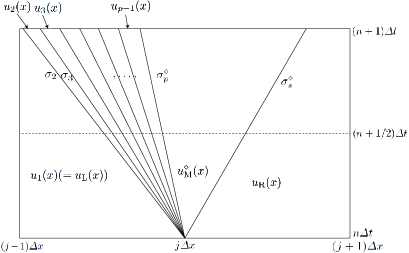
Figure 3. The approximate solution in the case where a 1-rarefaction and a 2-shock arise in the cell.

We denote this approximate Riemann solution, which consists of (3.9), by ${u}^{\varDelta}(x,t)$. The validity of the above construction is demonstrated in [T1, Appendix A].

Remark 3.1.

${u}^{\varDelta}(x,t)$ satisfies the Rankine–Hugoniot conditions at the middle time of the cell, $t_{\rm M}:=(n+1/2){\varDelta}t$.

Remark 3.2.

The approximate solution $u^{\varDelta}(x,t)$ is piecewise smooth in each of the divided parts of the cell. Then, in the divided part, $u^{\varDelta}(x,t)$ satisfies

$$(u^{\varDelta})_{t}+f(u^{\varDelta})_{x}-g(x,u^{\varDelta})=O(\varDelta x).$$

4. Energy inequality

In this section, we prove Theorem 1.2, i.e., we deduce an energy inequality for our solutions in Theorem 1.1. For any fixed $T>0$, we set $N=[T/\varDelta t]$, where $[x]$ is the greatest integer not greater than $x$. From (3.2) and finite propagation, we can choose ${R_{T}}$ large enough such that ${\rm Supp}\>u^{\varDelta}\subset[1,{R_{T}}]\times[0,T]$. Throughout this section, by Landau’s symbols such as $O({\varDelta}x)$, $O(({\varDelta}x)^{2})$ and $o({\varDelta}x)$, we denote quantities whose moduli satisfy a uniform bound depending only on $R_{T}$ and $M$ in (1.10).

From Remark 3.2, $u^{\varDelta}$ satisfy

$$\eta_{*}(u^{\varDelta})_{t}+q_{*}(u^{\varDelta})_{x}-a(x)q_{*}(u^{\varDelta})=O(\varDelta x)$$

on the divided part in the cell where $u^{\varDelta}$ are smooth. Moreover, $u^{\varDelta}$ satisfy an entropy condition (see [T1, Lemma 5.1–Lemma 5.4]) along discontinuous lines approximately. Then, applying the Green formula to $\eta_{*}(u^{\varDelta})_{t}+q_{*}(u^{\varDelta})_{x}-a(x)q_{*}(u^{\varDelta})$ in the cell $(j-1){\varDelta}x\leq{x}<(j+1){\varDelta}x,\;n{\varDelta}{t}\leq{t}<(n+1){\varDelta}{t}\quad(j\in J_{n+1},\;n\in{\bf Z}_{\geq 0},\;n\leq N)$, we have

$$\begin{split}\eta_{*}(u^{n+1}_{j})\leq&\frac{\eta_{*}(u^{n}_{j+1})+\eta_{*}(u^{n}_{j-1})}{2}-\frac{\varDelta t}{2\varDelta x}\left\{q(u^{n}_{j+1})-q(u^{n}_{j-1})\right\}\\ &+R(x^{n}_{j+1},u^{n}_{j+1}){\varDelta t}-R(x^{n}_{j-1},u^{n}_{j-1}){\varDelta t}\\ &+\frac{1}{2\varDelta x}\int^{t_{n+1}}_{t_{n}}\int^{x_{j+1}}_{x_{j-1}}\frac{A^{\prime}(x)}{A(x)}q(u^{\varDelta}(x,t))dxdt+o(\varDelta x),\end{split}$$ (4.1)

where $t_{n}=n{\varDelta t}$ and

$$R(x,u)= -\frac{\varDelta x}{4{\varDelta t}}b(x)\left(\frac{3}{\gamma-1}(\rho)^{\theta}m+\frac{m^{3}}{2(\rho)^{\theta+2}}\right)$$

$$+\frac{\varDelta t}{4\varDelta x}a(x)\left\{\frac{\gamma}{\gamma-1}\frac{\rho^{2\theta}m^{2}}{\rho}+\frac{1}{2}\frac{m^{4}}{\rho^{3}}\right\}$$

$$-\frac{\varDelta t}{4\varDelta x}b(x)\left\{\frac{\gamma+\theta+1}{(\gamma-1)\theta}m\rho^{3\theta}+\frac{\gamma+3\theta+4}{2\theta}\frac{m^{3}\rho^{\theta}}{\rho^{2}}+\frac{m^{5}}{2\rho^{\theta+4}}\right\}.$$

Multiplying the above inequality by $A(x)$, we obtain

$$\sum_{j\in J_{n+1}}\int_{I_{j}}A(x)\eta_{*}(u_{j}^{n+1})dx\leq A_{n}+B_{n}+C_{n}+o(\varDelta x),$$

where $I_{j}=[(j-1){\varDelta}x,(j+1){\varDelta}x]$ and

$$A_{n}= \sum_{j\in J_{n+1}}\int_{I_{j}}A(x)\frac{\eta_{*}(u^{n}_{j+1})+\eta_{*}(u^{n}_{j-1})}{2}dx-\sum_{j\in J_{n+1}}\int_{I_{j}}A(x)\frac{\varDelta t}{2\varDelta x}\left\{q(u^{n}_{j+1})-q(u^{n}_{j-1})\right\}dx,$$

$$B_{n}= -\frac{1}{2\varDelta x}\sum_{j\in J_{n+1}}\int_{I_{j}}A(x)\left\{\int^{t_{n+1}}_{t_{n}}\int^{x_{j+1}}_{x_{j-1}}\frac{A^{\prime}(y)}{A(y)}q(u^{\varDelta}(y,t))dydt\right\}dx,$$

$$C_{n}= \sum_{j\in J_{n+1}}\int_{I_{j}}A(x)\left\{R(x^{n}_{j+1},u^{n}_{j+1})-R(x^{n}_{j-1},u^{n}_{j-1})\right\}{\varDelta t}\>dx.$$

We first compute $A_{n}$.

$$A_{n}= \sum_{j\in J_{n+1}}\left\{\int_{I_{j+2}}A(x)dx+\int_{I_{j}}A(x)dx\right\}\frac{\eta_{*}(u^{n}_{j+1})}{2}$$

$$+\sum_{j\in J_{n+1}}\left\{\int_{I_{j+2}}A(x)dx-\int_{I_{j}}A(x)dx\right\}\frac{\varDelta t}{2\varDelta x}q(u_{j+1}^{n})$$

$$= \sum_{j\in J_{n}}\left\{\int_{I_{j+1}}A(x)dx+\int_{I_{j-1}}A(x)dx\right\}\frac{\eta_{*}(u^{n}_{j})}{2}dx$$

$$+\sum_{j\in J_{n}}\left\{\int_{I_{j+1}}A(x)dx-\int_{I_{j-1}}A(x)dx\right\}\frac{\varDelta t}{2\varDelta x}q(u_{j}^{n})$$

$$= \sum_{j\in J_{n}}\int_{I_{j}}A(x)\eta_{*}(u^{n}_{j})dx+{\varDelta t}\sum_{j\in J_{n}}\int_{I_{j}}A^{\prime}(x)q(u_{j}^{n})dx+O((\varDelta x)^{2}).$$

Next we compute $B_{n}$. Then we have

$$\begin{split}B_{n}=&-\frac{1}{2\varDelta x}\sum_{j\in J_{n+1}}\int_{I_{j}}A(x)\left\{\int^{t_{n+1}}_{t_{n}}\int_{I_{j}}\frac{A^{\prime}(y)}{A(y)}q(u^{\varDelta}(y,t))dydt\right\}dx\\ =&-\sum_{j\in J_{n+1}}\int^{t_{n+1}}_{t_{n}}\int_{I_{j}}A^{\prime}(x)q(u^{\varDelta}(x,t))dxdt+O((\varDelta x)^{2})\\ =&-{\varDelta t}\sum_{j\in J_{n+1}}\int_{I_{j}}A^{\prime}(x)q(u_{j}^{n+1})dx\\ &+\sum_{j\in J_{n+1}}\int^{t_{n+1}}_{t_{n}}\int_{I_{j}}A^{\prime}(x)\left\{q(u^{\varDelta}(x,t_{n+1}+0))-q(u^{\varDelta}(x,t_{n+1}-0))\right\}dxdt\\ &+\sum_{j\in J_{n+1}}\int^{t_{n+1}}_{t_{n}}\int_{I_{j}}A^{\prime}(x)\left\{q(u^{\varDelta}(x,t_{n+1}-0))-q(u^{\varDelta}(x,t))\right\}dxdt+O((\varDelta x)^{2})\\ :=&-{\varDelta t}\sum_{j\in J_{n+1}}\int_{I_{j}}A^{\prime}(x)q(u_{j}^{n+1})dx+D_{n}+E_{n}+O((\varDelta x)^{2}).\end{split}$$

Moreover, we find

$$C_{n}= -{\varDelta t}\sum_{j\in J_{n+1}}\left\{\int_{I_{j+2}}A(x)dx-\int_{I_{j}}A(x)dx\right\}R(x^{n}_{j+1},u^{n}_{j+1})$$

$$= -\varDelta x\>{\varDelta t}\sum_{j\in J_{n+1}}\int_{I_{j+1}}A^{\prime}(x)dxR(x^{n}_{j+1},u^{n}_{j+1})+O((\varDelta x)^{2})$$

$$= O((\varDelta x)^{2}).$$

Therefore, we have

$$\begin{split}\sum_{j\in J_{n+1}}\int_{I_{j}}A(x)\eta_{*}(u_{j}^{n+1})dx\leq&\sum_{j\in J_{n}}\int_{I_{j}}A(x)\eta_{*}(u_{j}^{n})dx-{\varDelta t}\sum_{j\in J_{n+1}}\int_{I_{j}}A^{\prime}(x)q(u_{j}^{n+1})dx\\ &+{\varDelta t}\sum_{j\in J_{n}}\int_{I_{j}}A^{\prime}(x)q(u_{j}^{n})dx+D_{n}+E_{n}+o(\varDelta x).\end{split}$$ (4.2)

Since $\eta_{*}$ is a convex function, from the Jensen inequality, we obtain

$$\begin{split}\sum_{j\in J_{n+1}}\int_{I_{j}}A(x)\eta_{*}(u_{j}^{n+1})dx&\leq\sum_{j\in J_{0}}\int_{I_{j}}A(x)\eta_{*}(u_{j}^{0})dx+\sum^{n}_{k=0}\left(D_{n}+E_{n}\right)+o(1)\\ &\leq\int_{\bf R}A(x)\eta_{*}(u_{0})dx+\sum^{n}_{k=0}\left(D_{n}+E_{n}\right)+o(1).\end{split}$$

Then, we introduce the following proposition:

Proposition 4.1.

$$\sum^{N-1}_{k=0}\int^{R_{T}}_{1}|\overline{u}^{\varDelta}(r,t_{k}-0)-\overline{u}^{\varDelta}(r,t_{k}+0)|^{2}dx\leq C,$$ (4.3)

$$\sum^{N}_{k=1}\int^{t_{k}}_{t_{k-1}}\int^{R_{T}}_{1}|\overline{u}^{\varDelta}(r,t_{k}-0)-\overline{u}^{\varDelta}(r,t)|^{2}dx=O(\varDelta x)$$ (4.4)

(4.3) and (4.4) can be obtained in a similar manner to [T1, (6.18)] and [T1, Lemma 7.1] respectively.

From the above propositions and the Schwarz inequality, we have

$$\sum^{n}_{k=0}\left(D_{n}+E_{n}\right)=O(\sqrt{\varDelta x}).$$

Therefore, it follows that

$$\sum_{j\in J_{n+1}}\int_{I_{j}}A(x)\eta_{*}(u_{j}^{n+1})dx\leq\int_{\bf R}A(x)\eta_{*}(u_{0})dx+o(1).$$

Next, let $s$ be any fixed positive value satisfying $t_{n}\leq s\leq\min\{t_{n+1},T\}$. Applying the Green formula to $\eta_{*}(u^{\varDelta})_{t}+q_{*}(u^{\varDelta})_{x}-a(x)q_{*}(u^{\varDelta})$ in the cell $(j-1){\varDelta}x\leq{x}<(j+1){\varDelta}x,\;{t}_{n}\leq{t}<{s}$, we have

$$\begin{split}\int_{I_{j}}\eta_{*}(u^{\varDelta}(x,s))dx\leq&\frac{\eta_{*}(u^{n}_{j+1})+\eta_{*}(u^{n}_{j-1})}{2}-\frac{s-t_{n}}{2\varDelta x}\left\{q(u^{n}_{j+1})-q(u^{n}_{j-1})\right\}\\ &+R(x^{n}_{j+1},u^{n}_{j+1})(s-t_{n})-R(x^{n}_{j-1},u^{n}_{j-1})(s-t_{n})\\ &+\frac{1}{2\varDelta x}\int^{s}_{t_{n}}\int^{x_{j+1}}_{x_{j-1}}\frac{A^{\prime}(x)}{A(x)}q(u^{\varDelta}(x,t))dxdt+o(\varDelta x).\end{split}$$

We deduce from the above inequality

$$\begin{split}\int_{\bf R}A(x)\eta_{*}(u^{\varDelta}(x,s))dx=&\sum_{j\in J_{n+1}}\int_{I_{j}}A(x)\eta_{*}(u^{\varDelta}(x,s))dx\\ \leq&\sum_{j\in J_{n}}\int_{I_{j}}A(x)\eta_{*}(u_{j}^{n})dx+O(\varDelta x)\end{split}$$ (4.6)

in a similar manner to (4.2).

Combining $(4.5)_{n}$ and (4.6), for $s\leq T$, we conclude

$$\begin{split}\int_{\bf R}A(x)\eta_{*}(u^{\varDelta}(x,s))dx\leq\int_{\bf R}A(x)\eta_{*}(u_{0})dx+o(1).\end{split}$$ (4.7)

Then, integrating (4.7) over the region $S\in{\bf R}_{+}$ with $0<\mu(S)<\infty$, we have

$$\begin{split}\int_{\bf R}\int_{S}A(x)\eta_{*}(u^{\varDelta}(x,s))dxds\leq\mu(S)\int_{\bf R}A(x)\eta_{*}(u_{0})dx+o(1),\end{split}$$ (4.8)

where $\mu$ is the one-dimensional Lebesgue measure.

By virtue of the methods of compensated compactness for the approximate solutions (see [T6]), there exists a subsequence $u^{\varDelta_{k}}$ such that $(\varDelta x)_{k}\rightarrow 0$ and $u^{\varDelta_{k}}$ tends to a weak solution to (1.1) almost everywhere $(x,t)\in{\bf R}_{+}\times{\bf R}$ as $k\rightarrow\infty$. Applying (4.8) to the above subsequence and taking the limit, we have

$$\begin{split}\frac{1}{\mu(S)}\int_{\bf R}\int_{S}A(x)\eta_{*}(u(x,s))dxds\leq\int_{\bf R}A(x)\eta_{*}(u_{0})dx.\end{split}$$ (4.9)

Recalling that $S$ are arbitrary, we have (1.11). Since we can obtain (1.11) for an arbitrary $X$ in (3.2), we conclude Theorem 1.2.

Appendix A Construction of Approximate Solutions near the vacuum

In this step, we consider the case where $\rho_{\rm M}\leq({\varDelta}x)^{\beta}$, which means that $u_{\rm M}$ is near the vacuum. In this case, we cannot construct approximate solutions in a similar fashion to Subsection 3.1. Therefore, we must define $u^{\varDelta}(x,t)$ in a different way.

In this appendix, we define our approximate solutions in the cell $(j-1){\varDelta}x\leq{x}<(j+1){\varDelta}x,\;n{\varDelta}{t}\leq{t}<(n+1){\varDelta}{t}\quad(j\in{\bf Z},\;n\in{\bf Z}_{\geq 0})$. We set $L_{j}:=-{M}e^{-\int^{(j+1){\varDelta}x}_{0}b(x)dx}$ and $U_{j}:={M}e^{\int^{j{\varDelta}x}_{0}b(x)dx}$.

Case 1 A 1-rarefaction wave and a 2-shock arise.

In this case, we notice that $\rho_{\rm R}\leq({\varDelta}x)^{\beta},\;z_{\rm R}\geq L_{j}$ and $w_{\rm R}\leq U_{j}$.

Definition of $\bar{u}^{\varDelta}$ in Case 1

Case 1.1 $\rho_{\rm L}>2({\varDelta}x)^{\beta}$

We denote $u^{(1)}_{\rm L}$ a state satisfying $w(u_{\rm L}^{(1)})=w(u_{\rm L})$ and $\rho^{(1)}_{\rm L}=2({\varDelta}x)^{\beta}$. Let $u^{(2)}_{\rm L}$ be a state connected to $u_{\rm L}$ on the right by $R_{1}^{\varDelta}(z^{(1)}_{\rm L})(u_{\rm L})$. We set

$$(z^{(3)}_{\rm L},w^{(3)}_{\rm L})=\begin{cases}(z^{(2)}_{\rm L},w(u_{\rm L})),\quad\text{if $z^{(2)}_{\rm L}\geq L_{j}$},\\ (L_{j},w(u_{\rm L})),\quad\text{if $z^{(2)}_{\rm L}<L_{j}$}.\end{cases}$$

Then, we define

$$\bar{u}^{\varDelta}(x,t)=\begin{cases}R_{1}^{\varDelta}(z^{(1)}_{\rm L})(u_{\rm L}),\quad\text{if $(j-1){\varDelta}x\leq{x}\leq{j}{\varDelta}x+\lambda_{1}(u^{(2)}_{\rm L})(t-n{\varDelta}t)$}\\ \text{and $n{\varDelta}t\leq{t}<(n+1){\varDelta}t$},\vspace*{2ex}\\ \text{a Riemann solution $(u^{(3)}_{\rm L}$, $u_{\rm R})$},\quad\text{if ${j}{\varDelta}x+\lambda_{1}(u^{(2)}_{\rm L})(t-n{\varDelta}t)$}\\ \text{$<x\leq(j+1){\varDelta}x$ and $n{\varDelta}t\leq{t}<(n+1){\varDelta}t$}.\end{cases}$$

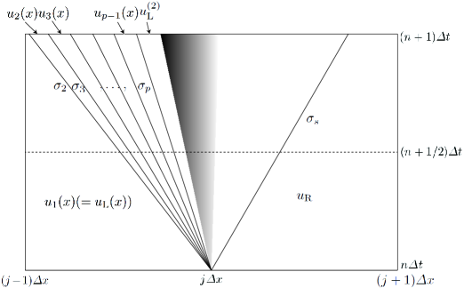
Figure 4. Case 1.1: The approximate solution $\bar{u}^{\varDelta}$ in the cell.

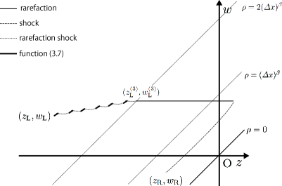
Figure 5. Case 1.1: The approximate solution $\bar{u}^{\varDelta}$ in $(z,w)-$plane.

Case 1.2 $\rho_{\rm L}\leq 2({\varDelta}x)^{\beta}$

(i) $z(u_{\rm L})\geq{L}_{j}$
In this case, we define $u^{\varDelta}(x,t)$ as a Riemann solution $(u_{\rm L},u_{\rm R})$.

(ii) $z(u_{\rm L})<L_{j}$
In this case, recalling $z(u_{\rm L})=z(u^{n}_{j})\geq-{M}e^{-\int^{j{\varDelta}x}_{0}b(x)dx}$, we can choose $x^{(4)}$ such that $(j-1){\varDelta}x\leq{x}^{(4)}\leq(j+1){\varDelta}x$ and $z(u_{\rm L})e^{-\int^{x^{(4)}}_{x_{\rm L}}b(x)dx}=L_{j},$ where $x_{\rm L}:=j{\varDelta}x$. We set

$$z^{(4)}_{\rm L}:=z_{\rm L}e^{-\int^{x^{(4)}}_{x_{\rm L}}b(x)dx},\quad{w}^{(4)}_{\rm L}:=w_{\rm L}e^{-\int^{x^{(4)}}_{x_{\rm L}}b(x)dx}.$$

In the region where $(j-1){\varDelta}x\leq{x}\leq{j}{\varDelta}x+\lambda_{1}(u^{(4)}_{\rm L})(t-n{\varDelta}t)$ and $n{\varDelta}t\leq{t}<(n+1){\varDelta}t$, we define $\bar{u}^{\varDelta}(x,t)$ as

$$\bar{z}^{\varDelta}(x,t)=z_{\rm L}e^{-\int^{x}_{x_{\rm L}}b(x)dx},\quad\bar{w}^{\varDelta}(x,t)=w_{\rm L}e^{-\int^{x}_{x_{\rm L}}b(x)dx}.$$ (A.1)

We next solve a Riemann problem $(u^{(4)}_{\rm L},u_{\rm R})$. In the region where ${j}{\varDelta}x+\lambda_{1}(u^{(4)}_{\rm L})(t-n{\varDelta}t)\leq{x}\leq(j+1){\varDelta}x$ and $n{\varDelta}t\leq{t}<(n+1){\varDelta}t$, we define $\bar{u}^{\varDelta}(x,t)$ as this Riemann solution.

We notice that the Riemann solutions in Case 1.2 are also contained in $\varDelta_{j}$.

Definition of ${u}^{\varDelta}$ in Case 1

In the region where $\bar{u}^{\varDelta}(x,t)$ is the Riemann solution, we define $u^{\varDelta}(x,t)$ by $u^{\varDelta}(x,t)=\bar{u}^{\varDelta}(x,t)$; in the region $\bar{u}^{\varDelta}(x,t)$ is (A.1), we define

$$\begin{split}z^{\varDelta}(x,t)=&\bar{z}^{\varDelta}(x)-\left\{a(x)\bar{v}^{\varDelta}(x)(\bar{\rho}^{\varDelta}(x))^{\theta}-b(x)\lambda_{1}(\bar{u}^{\varDelta}(x))\bar{z}^{\varDelta}(x)\right\}(t-n{\varDelta{t}}),\\ w^{\varDelta}(x,t)=&\bar{w}^{\varDelta}(x)+\left\{a(x)\bar{v}^{\varDelta}(x)(\bar{\rho}^{\varDelta}(x))^{\theta}+b(x)\lambda_{2}(\bar{u}^{\varDelta}(x))\bar{w}^{\varDelta}(x)\right\}(t-n{\varDelta{t}});\end{split}$$

otherwise, the definition of $u^{\varDelta}(x,t)$ is similar to Subsection 3.1. Thus, for a Riemann solution near the vacuum, we define our approximate solution as the Riemann solution itself.

Case 2 A 1-shock and a 2-rarefaction wave arise.

From symmetry, this case reduces to Case 1.

Case 3 A 1-rarefaction wave and a 2-rarefaction wave arise.

For $u_{\rm L}$ of Case 1, we define $u^{*}_{\rm L}$ and $\lambda^{*}_{\rm L}$ as follows.

$$u^{*}_{\rm L}=\begin{cases}u^{(3)}_{\rm L},\quad\text{Case 1.1},\\ u_{\rm L},\quad\text{Case 1.2 (i)},\\ u^{(4)}_{\rm L},\quad\text{Case 1.2 (ii)},\end{cases}\quad\lambda^{*}_{\rm L}=\begin{cases}\lambda_{1}(u^{(2)}_{\rm L}),\quad\text{Case 1.1},\\ \lambda_{1}(u_{\rm L}),\quad\text{Case 1.2 (i)},\\ \lambda_{1}(u^{(4)}_{\rm L}),\quad\text{Case 1.2 (ii)}.\end{cases}$$

where $\lambda_{1}(u)$ be the 1-characteristic speed of $u$. Then, for $u_{\rm L}$ of Case 3, we can determine $u^{*}_{\rm L}$ and $\lambda^{*}_{\rm L}$ in a similar manner to Case 1. From symmetry, for $u_{\rm R}$ of Case 3, we can also determine $u^{*}_{\rm R}$ and $\lambda^{*}_{\rm R}$.

In the region $(j-1){\varDelta}x\leq{x}\leq{j}{\varDelta}x+\lambda^{*}_{\rm L}(t-n{\varDelta}t),\;{j}{\varDelta}x+\lambda^{*}_{\rm R}(t-n{\varDelta}t)\leq{x}\leq(j+1){\varDelta}x$ and $n{\varDelta}t\leq{t}<(n+1){\varDelta}t$, we define $\bar{u}^{\varDelta}$ in a similar manner to Case 1. In the other region, we define $\bar{u}^{\varDelta}$ as the Riemann solution $(u^{*}_{\rm L},u^{*}_{\rm R})$.

We define ${u}^{\varDelta}$ in the same way as Case 1.

Case 4 A 1-shock and a 2-shock arise.

We notice that $z_{\rm L}\geq L_{j},\;w_{\rm L}\leq U_{j},\;z_{\rm R}\geq L_{j}$ and $w_{\rm R}\leq U_{j}$. In this case, we define $u^{\varDelta}(x,t)$ as the Riemann solution $(u_{\rm L},u_{\rm R})$. We notice that the Riemann solution is also contained in $\varDelta_{j}$.

We complete the construction of our approximate solutions.

References

- [CS] Chen G.-Q., Schrecker Matthew R. I.: Vanishing Viscosity Approach to the Compressible Euler Equations for Transonic Nozzle and Spherically Symmetric Flows. Arch. Ration. Mech. Anal. 229, 1239–1279 (2018)
- [L1] Liu, T.-P.: Quasilinear hyperbolic systems. Commun. Math. Phys. 68, 141–172 (1979)
- [L2] Lu, Y.-G.: Global existence of solutions to resonant system of isentropic gas dynamics. Nonlinear Anal. Real World Appl. 12, 2802–2810 (2011)
- [LG] Lu, Yun-guang, Gu, F.: Existence of global entropy solutions to the isentropic Euler equations with geometric effects. Nonlinear Anal. Real World Appl. 14, 990–996 (2013)
- [LW] Philippe G. LeFloch, Michael Westdickenberg: Finite energy solutions to the isentropic Euler equations with geometric effects. J. Math. Pures Appl. 88, 389-429 (2007)
- [MT] Makino, T. and Takeno,S.: Initial-boundary value problem for the spherical symmetric motion of isentropic gas. Jpn J. Ind. Appl. Math. 11, 171–183 (1994)
- [T1] Tsuge, N.: Global solutions of the compressible Euler equations with spherical symmetry. J. Math. Kyoto Univ. 46, 457–524 (2006)
- [T2] Tsuge, N.: Large time decay of solutions to isentropic gas dynamics. Quart. Appl. Math. 65, 135–143 (2007).
- [T3] Tsuge, N.: Large time decay of solutions to isentropic gas dynamics with spherical symmetry. J. Hyperbolic Differ. Equ. 6, 371–387 (2009).
- [T4] Tsuge, N.: Existence of global solutions for unsteady isentropic gas flow in a Laval nozzle. Arch. Ration. Mech. Anal. 205, 151–193 (2012)
- [T5] Tsuge, N.: Isentropic gas flow for the compressible Euler equation in a nozzle. Arch. Ration. Mech. Anal. 209, 365–400 (2013)
- [T6] Tsuge, N.: Global entropy solutions to the compressible Euler equations in the isentropic nozzle flow for large data: Application of the generalized invariant regions and the modified Godunov scheme. Nonlinear Anal. Real World Appl. 37, 217–238 (2017)
- [T7] Tsuge, N.: Isentropic Gas Flow in a Laval Nozzle: Physical Phenomena of Steady Flow and Time Global Existence of Solutions. RIMS Kôkyûroku 2070, 150–162 (2016) http://www.kurims.kyoto-u.ac.jp/ kyodo/kokyuroku/contents/2070.html