Dragging the roots of a polynomial to the unit circle

Abstract.

Several conditions are known for a self-inversive polynomial that ascertain the location of its roots, and we present a framework for comparison of those conditions. We associate a parametric family of polynomials $p_{\alpha}$ to each such polynomial $p$, and define $\text{c\!n}\!\mspace{-2.0mu}\left(p\right)$, $\text{i\!l}\!\mspace{-2.0mu}\left(p\right)$ to be the sharp threshold values of $\alpha$ that guarantee that, for all larger values of the parameter, $p_{\alpha}$ has, respectively, all roots in the unit circle and all roots interlacing the roots of unity of the same degree. Interlacing implies circle rootedness, hence $\text{i\!l}\!\mspace{-2.0mu}\left(p\right)\geq\text{c\!n}\!\mspace{-2.0mu}\left(p\right)$, and this inequality is often used for showing circle rootedness. Both $\text{c\!n}\!\mspace{-2.0mu}\left(p\right)$ and $\text{i\!l}\!\mspace{-2.0mu}\left(p\right)$ turn out to be semi-algebraic functions of the coefficients of $p$, and some useful bounds are also presented, entailing several known results about roots in the circle. The study of $\text{i\!l}\!\mspace{-2.0mu}\left(p\right)$ leads to a rich classification of real self-inversive polynomials of each degree, organizing them into a complete polyhedral fan. We have a close look at the class of polynomials for which $\text{i\!l}\!\mspace{-2.0mu}\left(p\right)=\text{c\!n}\!\mspace{-2.0mu}\left(p\right)$, whereas in general the quotient$\frac{\text{i\!l}\!\mspace{-2.0mu}\left(p\right)}{\text{c\!n}\!\mspace{-2.0mu}\left(p\right)}$ is shown to be unbounded as the degree grows. Several examples and open questions are presented.

1. Introduction

There is considerable interest in polynomials that have all of their roots on the real line (real rooted polynomials) or on the unit circle (circle rooted polynomials). From one perspective, the two classes are the same: a Möbius transformation mapping the real line to the circle minus a point essentially maps real rooted polynomials to circle rooted polynomials. This well-known connection will be explored further in section 6, but it is far from the whole story.

One can envision two classes of results in this theme of real and circle rootedness. In the first class, specific families of polynomials are considered, and then it is shown that some values of the parameters imply the desired root location. For real rooted polynomials there are many classical families of orthogonal polynomials and several polynomials arising in Combinatorics, either as counting functions or as generating functions ([11],[5], [34], [6]). For circle rooted polynomials, such families are somewhat less common (see [14], [27], [26], [1], [4], [28]).

In the second class, some conditions on the coefficients implying the root location are described. There are some results of this type for real rooted polynomials, as in [20]. For circle rooted polynomials, however, there are plenty of sufficient conditions of this kind on the coefficients ([24, 22, 25, 23], [10], [21]), and some of them have been used as tools for results in the first class. This paper lies in this second class, but has a thoroughly different viewpoint on circle rooted polynomials and a new perspective on the results in some of the cited papers. To present it, we discuss a little more some of those results.

Let us for a moment forbid $1$ as a root of a polynomial. The most basic necessary condition for a real degree $n$ polynomial

$$p(x)=a_{0}+a_{1}x+\cdots+a_{n}x^{n}$$

to be circle rooted is that $a_{k}=a_{n-k}$ for all $k$; equivalently, as rational functions, $p(x)=x^{n}p\left(\frac{1}{x}\right)$. Now we reinstate $1$ as a kosher root, but demand that it appears with even multiplicity; in this way, the necessary condition persists. Those polynomials have been called palindromic or reciprocal; we opt for palindromic.

Another motivation for this type of polynomials comes from the problem of counting the zeros of a given complex polynomial in the unit disk. It refers to an appropriate generalization of palindromic polynomial: a complex $p(x)$ is self-inversive if $p(x)=x^{n}\bar{p}\left(\frac{1}{x}\right)$. A symmetrization technique developed by Cohn (see [32, sect. 11.5], and a recent strengthening by [27]) essentially moves that counting problem to that of counting the number of roots of a self-inversive polynomial in the unit circle, and to being able to verify whether such a polynomial is circle rooted. [40] surveys self-inversive and palindromic polynomials from a viewpoint that is entirely germane to this paper, while [19] give some a priori reasons for considering these kinds of polynomials.

Many of the methods and results to be presented here work for self-inversive polynomials and will be shown as such. However, it is important to keep in mind that our focus in this paper is real palindromic polynomials (wich are the self-inversive ones with real coefficients), with self-inversive ones being taken along for the ride, and only so long as the additional generality comes at near zero cost. One can always multiply a palindromic polynomial by a scalar so that if becomes monic - and it keeps being palindromic; that is not true for self-inversive polynomials in general. So, for palindromic polynomials there is a natural special role for the polynomials $x^{n}+1$ and for the roots of unity; forcing them upon self-inversive ones is expedient and yields nontrivial results, but it is not exactly the “right” theory. So, the discussion that follows will concern real palindromic polynomials, but some of the main results in Sections 2, 4 and 6 are proved for self-inversive polynomials.

A very simple way of showing that a degree $n$ polynomial $p$ is real rooted is to present a sequence $a_{1}<a_{2}<\cdots<a_{n-1}$ such that the values $p(a_{i})$ alternate in sign; $p$ is said to sign-interlace the sequence. Provided $p(a_{n-1})$ has sign opposite to that of the leading term of $p$, the polynomial will have roots $x_{1}<x_{2}<\cdots<x_{n}$ such that $x_{1}<a_{1}<x_{2}<a_{2}<\cdots<a_{n-1}<x_{n}$, that is, the $x_{i}$’s and $a_{i}$’s interlace. Indeed, the main technique for proving that a polynomial is real rooted is to make it part of a recursive sequence, each member of it sign-interlacing the next one. As a general technique, see [16, 1.14 ], [41]. For any given polynomial, the Sturm sequence (see [3]) fulfills this role, if the polynomial is real rooted.

Moving now to the complex plane, there is a geometrically motivated notion: start with a set $A=\{a_{1},\ldots,a_{n}\}$ of points in the unit circle and divide the complex plane into $n$ open angular sectors by half-lines from the origin, which pass through each point in $A$. We say that the polynomial $p$ strictly angle-interlaces $A$ if it has one root in each of those sectors. These elementary concepts come together in:

Proposition 3.3.

If a degree $n$ self-inversive polynomial strictly angle-interlaces a set of size $n$, then the polynomial is circle rooted.

Angle-interlacing sets in the unit circle have also been said to be interspersed (as in [37]). Although any set of $n$ points in the unit circle works for the purpose of showing that the polynomial is circle-rooted, there is one that stands out, in the case of palindromic polynomials, namely the set $U_{n}$ of $n$th roots of unity, and we claim that this is because they are “exactly” angle interlaced by the roots of $x^{n}+1$. Most of the preceding references prove circle rootedness in tandem with angle-interlacing with $U_{n}$. This is not just a coincidence; we will present a fairly simple way of checking angle-interlacing with $U_{n}$ that touches on the polynomial’s Fourier transform.

Our main motivating question derives from the idea of giving interlacing the status of first-class target, instead of a happenstance bonus:

Is looking for good conditions for angle-interlacing with $U_{n}$ a good strategy for nailing down circle rootedness?

We introduce numerical tools that allow us to treat this question in quantitative terms.

Monic palindromic polynomials look like $x^{n}+1+p(x)$, and suggest the following idea. The palindromic polynomial $x^{n}+1$ is trivially circle rooted and strictly angle-interlaces $U_{n}$; the latter property is open, hence all “sufficiently close” polynomials will also have it. We can look at $p(x)$ as a perturbation of $x^{n}+1$, and consider, for real $\varepsilon$, the polynomial $x^{n}+1+\varepsilon p(x)$, asking how small $\varepsilon$ has to be for angle-interlacing and circle rootedness to set in. It turns out to be more convenient to scale the parametric polynomial by $\alpha=1/\varepsilon$, and define, for any complex polynomial $p$ of degree at most $n$, the family

(1) $$p_{\alpha}(x)=\alpha(x^{n}+1)+p(x),$$

where $\alpha$ is a positive real parameter. Then, for a sufficiently large $\alpha$, $p_{\alpha}$ angle-interlaces $U_{n}$. We actually like the image of $\alpha$ dragging the roots of $p_{\alpha}$ until they latch on the unit circle, and then spread out to the slots provided by the roots of unity.

Let $p(x)=a_{r}x^{r}+a_{r+1}x^{r+1}+\cdots+a_{s}x^{s}$ be a nonzero polynomial, with $a_{r},a_{s}\neq 0$. In order to also handle polynomials of this form with no constant term, we follow [42] and define the darga of $p$ to be

(2) $$\mathrm{dg}\!\left(p\right)=r+s.$$

We say that a complex polynomial $p$ of darga $n$ is self-inversive if $x^{n}p\left(\frac{1}{x}\right)=\bar{p}(x)$; that means <$p_{j}=\bar{p}_{n-j}$ for all coefficients $p_{j}$. For real polynomials that reads $p_{j}=p_{n-j}$, justifying the term palindromic. If the darga equals the degree, we say that $p$ is full; otherwise, we call $p$ a trim polynomial. Most of the concepts and results in this article revolve around trim polynomials. If $p$ is self-inversive, we define its trimmed part by $\operatorname{trim}p=p(x)-\bar{p}(0)x^{\mathrm{dg}\!\left(p\right)}-p(0)$. One simple property that is good to keep in mind is that $p$ is palindromic and $\omega$ is in the unit circle, then $p(\omega)$ is real; this is not generally true for self-inversive polynomials, but holds if $\omega\in U_{n}$.

Now we can present the two main quantities we will be exploring. We define, for a trim self-inversive polynomial $p$:

• interlace number
  $\text{i\!l}\!\mspace{-2.0mu}\left(p\right)=\inf\left\{\left.\alpha>0\,\right|\;p_{\alpha}(x)\,\text{angle interlaces $U_{n}$}\right\}\text{, and}$

• circle number
  $\text{c\!n}\!\mspace{-2.0mu}\left(p\right)=\inf\left\{\left.\alpha>0\,\right|\;p_{\beta}(x)\,\text{is circle rooted for all}\ \beta>\alpha\right\}.$

Note the discrepancy between the definitions. It turns out that if $p_{\alpha}$ angle interlaces $U_{n}$, then so does $p_{\beta}$ for all $\beta>\alpha$. The same does not happen for the property of being circle-rooted (Example 6.3), so the definition of circle number has to be formally more complicated, to capture what we want, foreshadowing its inherent complexity. We could write the definition of i​l to parallel that of c​n, but not the other way around.

Those quantities allows one to rewrite and compare previously published facts (see Theorems 4.6, 4.7 and 9.7). Many theorems about circle-rootedness have the following form (where we identify a trim polynomial $\sum_{j=1}^{n-1}p_{j}x^{j}$ with the vector $(p_{1},\ldots,p_{n-1})$):

A class $\mathscr{F}$ of full palindromic polynomials, and functions $h_{n}:\mathbb{R}^{n-1}\rightarrow\mathbb{R}_{+}$ for each $n$ are specified. It is asserted that if $p\in\mathscr{F}$ has degree $n$ and is such that its leading coefficient is real and at least $h_{n}(\operatorname{trim}p)$, then $p$ is circle-rooted. Some statements come with a proviso that the roots also angle-interlace $U_{n}$ (for self-inversive polynomials, an appropriate rotation of $U_{n}$, instead).

Such a fact can be restated, taking $\mathscr{F^{\prime}}=\left\{\left.\operatorname{trim}p\,\right|\;p\in\mathscr{F}\right\}$, as:

A class $\mathscr{F^{\prime}}$ of trim palindromic polynomials, and functions $h_{n}:\mathbb{R}^{n-1}\rightarrow\mathbb{R}_{+}$ for each $n$ are specified. It is asserted that if $p\in\mathscr{F^{\prime}}$ has darga $n$ then $\text{c\!n}\!\mspace{-2.0mu}\left(p\right)\leq h_{n}(p)$ (or the stronger conclusion $\text{i\!l}\!\mspace{-2.0mu}\left(p\right)\leq h_{n}(p)$).

The existence of $\text{i\!l}\!\mspace{-2.0mu}\left(p\right)$ follows from the topological argument about proximity to $x^{n}+1$. Proposition 3.3 trivially implies that $\text{c\!n}\!\mspace{-2.0mu}\left(p\right)$ also exists and that we have the following simple relation between them.

Proposition 3.4.

$\text{c\!n}\!\mspace{-2.0mu}\left(p\right)\leq\text{i\!l}\!\mspace{-2.0mu}\left(p\right)$.

Moreover, a simple argument (Proposition 6.1) shows that both numbers are strictly positive.

These concepts provide a unifying framework for many of the articles cited here; several known theorems about circle rootedness can be reinterpreted as giving an upper bound for the interlace number or for the circle number.

The paper proceeds as follows. In Section 2 we present a quick background on interlacing. This is continued in Section 3, where angle-interlacing and self-inversive polynomials are discussed. Theorem 3.7 shows that one can find out whether a full monic self-inversive polynomial angle interlaces $U_{n}$ by computing the discrete Fourier transform of its coefficients.

Theorem 3.7.

Let $p(x)$ be a full monic self-inversive polynomial of degree $n$, with $p(1)>0$. Then $p(x)$ strictly angle-interlaces $U_{n}$ if and only if

$$\quad p(\omega)>0\quad\text{for all}\quad\omega\in U_{n}.$$

Section 4 starts an account of the interlace number. The main result in this section is the following formulation for the interlace number, in terms of the finite Fourier transform of the coefficients of $p$.

Theorem 4.2 ( Interlace formula).

If $p$ is a trim self-inversive polynomial of darga $n$, then

$$\quad\text{i\!l}\!\mspace{-2.0mu}\left(p\right)=\frac{1}{2}\max\left\{\left.-p(\omega)\,\right|\;\omega\in U_{n}\right\}.$$

This result and some variations entail short proofs of some criteria for circle rootedness in the literature that also yielded interlacing with $U_{n}$. It turns out that, for several parameterized families of polynomials, we can provide simple formulas for the interlace number, based on the parameters.

For each trim palindromic polynomial $p$, the maximum that determines $\text{i\!l}\!\mspace{-2.0mu}\left(p\right)$ is attained at a root of unity in the closed upper half-plane. Such a root we call an interlace cert, and there may be many. The trim palindromic polynomials of darga $n$ form a vector space of dimension $\left\lfloor n/2\right\rfloor$; those with a given interlace cert form a convex simplex cone, and the collection of these cones comprises a complete polyhedral fan. That Fan of Interlace Certs is depicted in detail in Section 5, along with a full description of its very large group of isometries.

Section 6 discusses the circle number, which turns out to be a more elusive concept than the interlace number. In this section, we use a different mapping of the circle to the real line, namely a Möbius transformation, making the proofs fully algebraic.

Theorem 6.7 (Double-root formula).

For a trim self-inversive polynomial $p$ of darga $n$, $\text{c\!n}\!\mspace{-2.0mu}\left(p\right)$ is the largest value of $\alpha$ for which $\frac{p_{\alpha}(x)}{\gcd(p(x),x^{n}+1)}$ has a double root.

This implies that the circle root can be computed by first calculating the discriminant of a polynomial, and then finding its largest real root, as a polynomial in $\alpha$. This is indeed quite effective in practice, for any given numerical polynomial. However, in contrast with what was achieved for the interlace number, giving nontrivial bounds for the circle number of polynomial families is a hard challenge.

Section 7 is the culmination of this work, where we compare the two numbers and see more precisely to what extent the interlace number approximates the circle number, thus directly addressing our main question. On the one hand, we show several sufficient conditions for these two numbers to coincide, and argue that the so-called exact polynomials form a class worthy of further attention, in particular because for that class the strategy underlying the main question is indeed optimal. On the other hand, in Theorem 7.7 we show that the numbers can grow unboundedly apart. More precisely, we define the bounding error

$$\text{b\!e}\!\mspace{-1.5mu}\left(p\right)=\frac{\text{i\!l}\!\mspace{-2.0mu}\left(p\right)}{\text{c\!n}\!\mspace{-2.0mu}\left(p\right)}-1,$$

and show that, while it is bounded when restricted to polynomials of a fixed darga, it is unbounded overall.

Finally, in the last two sections we have a more specialized look at those numbers. In Section 8 we investigate polynomials of small degrees, giving a concrete feeling for how these numbers behave. And, in Section 9 we look at some parameterized families and at other circle rootedness results from the viewpoint raised in this article.

The research carried out here was enabled by the use of SageMath [33], which helped us in developing and testing all sorts of wild conjectures. A few of these conjectures just turned out to be true and are presented here as theorems. Many results presented here (like Theorems 4.2 and 6.9) lead to algorithms that are straightforward to implement in the standard SageMath environment.

In this text, “self-inversive” is code for polynomials with possibly complex coefficients, while “palindromic” implies real. It turns out that one could restrict everything to polynomials over the (real) algebraic numbers. Indeed, $\text{i\!l}\!\mspace{-2.0mu}\left(p\right)$ is a piecewise-linear function; $\text{c\!n}\!\mspace{-2.0mu}\left(p\right)$ is far from that, but still is a semi-algebraic function of the real and imaginary parts of the coefficients of $p$. Some other interesting sets of polynomials presented here are, like the exact polynomials, also semi-algebraic. We will not delve deeply into this aspect, which surely deserves a better and more knowledgeable attention, but will point out the connection here and there. We refer to the book by [3] for the relevant definitions and results.

Several concepts and some notation will be defined as depending on a parameter $n$. As a rule, whenever $n$ is understood from the context, it will be omitted both in terminology and notation, or added as a superscript as in $\mathscr{T}^{(n)}$. Three frequently used symbols will always carry their $n$:

$$\theta_{n} =\IfSubStr{;n}{;}{\text{e}^{\frac{2\pi i\StrBefore{;n}{;}}{\raisebox{2.0pt}{$\scriptscriptstyle\StrBehind{;n}{;}$}}}}{\text{e}^{2i\pi;n}},$$

$$U_{n} =\left\{\left.{\theta_{n}\!}^{k}\,\right|\;0\leq k<n\right\}, n 1$$ the set of th roots of ,

$$V_{n} =\left\{\left.{\theta_{n}\!}^{k}\,\right|\;0\leq k\leq n/2\right\},$$ the roots with non negative imaginary part.

Also, in many statements there will appear an unqualified entity $p$; that will always be a trim polynomial of darga $n$. Repetition of this is too soporific, so we only do it in the more important statements.

2. Interlacing

There is a vast literature on interlacing polynomials, much of which has been collected by [16], in a book which was, unfortunately, unfinished. We present some notions here.

Let $A=\{a_{1}\leq a_{2}\leq\cdots\leq a_{n}\}$ and $B=\{b_{1}\leq b_{2}\leq\cdots\leq b_{m}\}$ be non decreasing sequences of real numbers; they interlace if they can be merged into $\{c_{1}\leq c_{2}\leq\cdots\leq c_{n+m}\}$, where the $c_{j}$’s alternate between $a$’s and $b$’s. In particular, $A$ interlaces itself. Notice that this requires that $n$ and $m$ differ by at most $1$; also, if a value appears twice in one sequence, it must also appear in the other one. If all those $n+m$ numbers are distinct, we say that $A$ and $B$ strictly interlace; alternatively, two sequences strictly interlace if they are both strictly increasing and between each pair of successive members of each there lies exactly one of the other.

A polynomial is said to be real rooted if its coefficients and all its roots are real; such a polynomial will be taken as a proxy for the ordered sequence of its roots with multiplicity. So, we will talk about polynomials interlacing, or a polynomial interlacing a sequence, keeping in mind that the zeros of the polynomial(s) are the issue.

A real polynomial $f(x)$ is said to sign-interlace a sequence of real numbers $A$ if the values $f(a_{j})$ are nonzero and alternate in sign.

The following are easy exercises:

Proposition 2.1.

(see [16, Lemma 1.9]) If $f(x)$ is a degree $n\geq 2$ real polynomial, and $A$ is a set of real numbers of size $n$, then $f(x)$ has $n$ real roots strictly interlacing $A$ if and only if it sign-interlaces $A$.

Proposition 2.2.

A real polynomial strictly interlaces a sequence $A$ of $n$ distinct real numbers if and only if it sign-interlaces $A$ and has at most $n+1$ real zeros.

This motivates the following definition that will be useful: a continuous function sign-interlaces $A$ if its values on $A$ alternates in sign. Clearly, such a function has at least $n-1$ zeros. We will use this exactly once.

A sequence $C$ is a common interlace to sequences $A$ and $B$ if it interlaces with both of them. The following is a simplified version of Prop. 1.35 in [16], also slightly generalized so that is applies to some polynomials with multiple roots:

Proposition 2.3.

Let $p,q$ be coprime polynomials of degree $n$ and positive leading coefficient; suppose also that $q$ has $n$ distinct real roots. Then $p_{\lambda}=(1-\lambda)p+\lambda q$ is real rooted for all $0<\lambda\leq 1$ if and only if $p$ is real rooted, and $p$ and $q$ have a common interlace. In this case, $p_{\lambda}$ has $n$ distinct roots for $0<\lambda<1$.

Proof.

Let us notice first that if $p$ has a nonreal root, then, by continuity of roots, so does $p_{\lambda}$ for $\lambda$ close to 0. So, real rootedness of $p$ is necessary for the whole setup.

We consider first the simpler case where $p$ also has $n$ real roots. Suppose that $C=\{c_{1}<\ldots<c_{n-1}\}$ is a common interlace to $p$ and $q$. Since the polynomials have positive leading coefficients, they are negative on $c_{n-1}$, so they have the same sign on all $c_{j}$. It follows that all convex combinations of $p$ and $q$ sign-interlace $C$ and have positive leading coefficient, therefore have $n$ real roots.

In general, let $A=\{a_{1}\leq a_{2}\leq\cdots\leq a_{n}\}$ be the roots of $p$, and $B=\{b_{1}<b_{2}<\cdots<b_{n}\}$ be the roots of $q$, and, for convenience, define $a_{n+1}=b_{n+1}=\infty$. The coprime hypothesis implies that $A$ and $B$ have no element in common. If $a_{j}=a_{j+1}$, then $c_{j}=a_{j}$; as $C$ interlaces $B$, it follows that $c_{j}<c_{j+1}\leq a_{j+2}$, implying that no root of $p$ has multiplicity higher than $2$. Also, if some $c_{k}$ is not a double root of $p$, we can move it a bit so as not to coincide with either $a_{i}$ or $b_{i}$, maintaining that $C$ still interlaces both polynomials; so, we may assume that unless $c_{k}$ is a double root of $p$, both $p(c_{k})$ and $q(c_{k})$ are nonzero. Now, $q$ has constant sign on each open interval between successive roots, and these signs alternate. The same happens to $p$, except in the degenerate case of a double root, but in this case $p$ has the same sign in the two adjacent intervals.

Let us show that they have the same sign. We do it by induction, descending from $n-1$. Since $p$ and $q$ have positive leading coefficients, they are both positive on the intervals $(a_{n},a_{n+1})$, $(b_{n},b_{n+1})$, respectively. It follows from the preceding paragraph that for every $k$, either $p$ and $q$ have the same sign in the intervals $(a_{k},a_{k+1})$, $(b_{k},b_{k+1})$, or $b_{k}$ is a double root of $p$. Since $c_{k}\in[a_{k},a_{k+1}]\cap[b_{k},b_{k+1}]$, it follows that, for $0<\lambda<1$, $p_{\lambda}$ sign-interlaces $C$, so it has $n$ distinct real roots.

Conversely, suppose $p_{\lambda}$ has $n$ real roots for all $0\leq\lambda\leq 1$. We claim that for $0<\lambda<1$, no root of $p$ or $q$ is a root $p_{\lambda}$. Indeed, if it was not the case, that root would be a common root of $p$ and $q$, contradicting the hypothesis that they are coprime. Now, it is well known that the roots of $p_{\lambda}$ depend continuously on $\lambda$, so each root of $q$ starts a path in the real line that ends on a root of $p$. Since that path contains no root of $p$ or $q$, it must be a segment, and by the same argument, these segments are interiorly disjoint. Any choice of points separating these segments will be a common interlace. ∎

Whereas the convex combination form is more convenient for the proof, the following will be more convenient for our purposes:

Proposition 2.4.

Let $p,q$ be coprime polynomials of degree $n$ and positive leading coefficient; suppose also that $q$ has $n$ distinct real roots. Then $p+\alpha q$ is real rooted for all $\alpha>0$ if and only if $p$ is real rooted, and $p$ and $q$ have a common interlace. In this case, then $p+\alpha q$ has $n$ distinct roots for all $\alpha>0$.

Proof.

Defining $\lambda=\frac{\alpha}{1+\alpha}$ land us back in Proposition 2.3. ∎

The following nonconstructive existence result is immediate:

Corollary 2.5.

Let $p,q$ be coprime real polynomials of degree $n$ and positive leading coefficient, each with $n$ real roots. If they have no common interlace, then there is a positive real $\alpha$ such that $p+\alpha q$ has a complex, nonreal root.

We will be interested on the dynamics of the set of real roots of $p_{\alpha}$, viewing $\alpha$ as the time variable. There is a ready tool for that, at least for counting those roots, using the classical subresultants. We refer the reader to [3, Chapter 4] for a full account and the definitions we use here; they are not going to be used beyond this paragraph, and are certainly not central to this paper. Consider a two variable polynomial $p(\alpha,x)\in\mathbb{R}[\alpha][x]$ as a family of polynomials on $x$ of generic degree $n$ parameterized by $\alpha$. Let $\text{sDisc}(p)=\left(\text{sDisc}_{0}(p),\ldots,\text{sDisc}_{n-1}(p)\right)$ be the sequence of subdiscriminants of $p$, each one a polynomial on $\alpha$. It follows from [3, Thm. 4.33] that, given $\alpha_{0}$, the number of real roots of $p(\alpha_{0},x)$ can be gleaned from the sequence of signs of the sequence $(\text{sDisc}_{0}(p)(\alpha_{0}),\ldots,\text{sDisc}_{n-1}(p)(\alpha_{0}))$. As the sign of a polynomial only changes around a zero of odd multiplicity, we can observe how the number of real roots of $p(\alpha,x)$ changes by the following procedure, which can be easily implemented, modulo the usual difficulties of representing real numbers:

1. Compute the sequence $\text{sDisc}(p)$. All terms are determinants of matrices which can be simply written given $p$.

2. Let $\alpha_{0}<\alpha_{1}<\ldots<\alpha_{m}$ be the collection of all roots of odd multiplicity of members $\text{sDisc}(p)$. Let $\alpha_{-1}=-\infty$, $\alpha_{m+1}=\infty$.

3. Within successive $\alpha_{j}$, all $p(\alpha,x)$ have the same number of real roots.

3. Palindromic polynomials

We recall some definitions. Let $p(x)=p_{r}x^{r}+p_{r+1}x^{r+1}+\cdots+p_{s}x^{s}$ be a nonzero polynomial, with $p_{r},p_{s}\neq 0$; the darga of $p$ is $\mathrm{dg}\!\left(p\right)=r+s$. We say that a polynomial $p$ of darga $n$ is self-inversive if $x^{n}\bar{p}(\frac{1}{x})=p(x)$; equivalently, if for all $j$, $p_{j}=\overline{p_{n-j}}$. If $p$ is self-inversive and has real coefficients, $p_{j}=p_{n-j}$ for all $j$, and we prefer the term palindromic. If the darga equals the degree, we say that $p$ is full, and it is trim otherwise. We denote the set of real palindromic polynomials of darga $n$ by $\mathscr{P}^{(n)}$, and the trim ones by $\mathscr{T}^{(n)}$; the corresponding sets of self-inversive polynomials will be $C\!\mathscr{P}^{(n)}$ and $C\!\mathscr{T}^{(n)}$. Note that all those sets are just short the zero polynomial of being real vector spaces, and it is convenient to complete them so, with a $0$ vector of each darga.

Proposition 3.1.

Let $p(x)$ be a full palindromic polynomial of degree $n$. Then:

1. If $p(x)=q(x)r(x)$ and $q(x)$ is palindromic, then so is $r(x)$.

2. If $\theta$ is a root of $p$, so are $\bar{\theta}$, $1/\theta$, $1/\bar{\theta}$. These four roots are distinct, unless $\theta$ lies in the circle or is real.

3. If $p$ is circle rooted, the only possible real roots are $1$, with even multiplicity, and $-1$, whose multiplicity has the same parity as $n$.

Proof.

This is mostly immediate from the definition. We only comment about the multiplicities of $\pm 1$. We can write $p(x)=(x-1)^{a}(x+1)^{b}q(x)$, where $q$ has no real roots. By part (2), $q$ is palindromic, and by part (1), so is $(x-1)^{a}(x+1)^{b}$; this clearly requires that $a$ be even. Also by part (2), $q$ has even degree, so the assertion about $b$ follows. ∎

For self-inversive polynomials we can say slightly less, but part (b) is the main reson for concentrating on self-inversive polynomials.

Proposition 3.2.

Let $p(x)$ be a full self-inversive polynomial of degree $n$. Then:

1. If $p(x)=q(x)r(x)$ and $q(x)$ is self-inversive, then so is $r(x)$.

2. If $\theta$ is a root of $p$, so is $1/\bar{\theta}$. These two roots are distinct, unless $\theta$ lies in the circle.

3. If $n$ is odd, -1 is a root of $p$.

4. If $\theta\in U_{n}$, then $p(\theta x)$ is self-inversive.

Proof.

Parts (a),(b) and (c) follow easily from the algebraic definition of self-inversive, while (d) comes from looking at coefficients. ∎

Darga $n$ palindromic polynomials form a subspace of the much larger space of polynomials of degree at most $n$, and, in this sense, the coefficients are the coordinates in the canonical basis of the large space, which is isomorphic to $\mathbb{R}^{n+1}$. The space $\mathscr{P}^{(n)}$ is much smaller, and it will be useful to use the $\sigma\!$-basis

(3) $$\left\{\left.\sigma\!_{n,j}(x)\,\right|\;j=0,1,\ldots,\left\lfloor n/2\right\rfloor\right\},$$

where

(4) $$\sigma\!_{n,j}(x):=x^{j}+x^{n-j}.$$

Notice that $\sigma\!_{2n,n}(x)=2x^{n}$. To summarize, if $p(x)=\sum_{j=0}^{n}p_{j}x^{j}$, then we define its $\sigma\!$-representation to be

(5) $$p(x)=\sum_{j=0}^{\left\lfloor n/2\right\rfloor}\tilde{p}_{j}\sigma\!_{n,j}(x),$$

where each $\sigma\!$-coefficient $\tilde{p}_{j}$ equals $a_{j}$, except if $n=2j$, in which case $\tilde{p}_{j}=p_{j}/2$. The space $\mathscr{T}^{(n)}$ of trim polynomials is spanned by $\sigma\!_{n,1},\ldots,\sigma\!_{n,\lfloor n/2\rfloor}$. The parity of $n$ will be of relevance in many results yet to appear; as above, the middle coefficient, for even $n$, often deserves special attention. So, to simplify some statements, we will adopt the convention

• any condition involving the middle coefficient $p_{n/2}$ implicitly carries the proviso “if $n$ is even”, and is vacuously true for odd $n$.

For instance, we can simply write $\tilde{p}_{n/2}=\frac{1}{2}p_{n/2}$.

Any complex polynomial can be written as $p(x)=p^{R}(x)+ip^{I}(x)$, where $p^{R}$ and $p^{I}$ are real polynomials. If $p$ is self-inversive, then $p^{R}$ is palindromic, while $p^{I}(x)=-x^{n}\bar{p}^{I}(1/x)$, that is, $p^{I}$ is anti-palindromic. A natural basis for anti-palindromic polynomials is

(6) $$\left\{\left.\hat{}\sigma\!_{n,j}(x)\,\right|\;0\leq j<n/2\right\},$$

where

(7) $$\hat{}\sigma\!_{n,j}(x):=x^{j}-x^{n-j}.$$

We extend the $\sigma\!$-representation to self-inversive polynomials, writing

(8) $$p(x)=\sum_{j=0}^{\left\lfloor n/2\right\rfloor}\tilde{p}_{j}\sigma\!_{n,j}(x)+i\!\!\!\!\!\sum_{j=0}^{\left\lfloor(n-1)/2\right\rfloor}\hat{p}_{j}\hat{}\sigma\!_{n,j}(x).$$

The notion of angle-interlacing will allow us to transfer some of the results from Section 2 to $C\!\mathscr{P}^{(n)}$. Given sequences of nonzero complex numbers, with nondecreasing arguments in the interval $[0,2\pi)$, $A=\{a_{1},a_{2},\cdots,$ $a_{n}\}$ and $B=\{b_{1},b_{2},\cdots,b_{n}\}$ of same length, we say that they angle-interlace if they can be merged into $\{c_{1},c_{2},\cdots,c_{n+m}\}$, where the $c_{j}$’s alternate between $a$’s and $b$’s and arguments are still nondecreasing; if all arguments are different, the sequences strictly angle-interlace. Geometrically, in the strict case, we think of the rays emanating from the origin through the points in $A$ and dividing the complex plane into $n$ sectors, with one element of $B$ in each sector. In the context of angle-interlacing, a polynomial will be considered a proxy for the adequate sequence of its roots with multiplicity, so we may speak about polynomials angle-interlacing.

We will use the exponential map $\exp(x)=\IfSubStr{x}{;}{\text{e}^{\frac{2\pi i\StrBefore{x}{;}}{\raisebox{2.0pt}{$\scriptscriptstyle\StrBehind{x}{;}$}}}}{\text{e}^{2i\pi x}}$, from the real interval $[0,1)$ to the unit circle $\mathbb{T}=\left\{\left.z\in\mathbb{C}\,\right|\;|z|=1\right\}$. Note that for every $x$, $\exp(-x)$ is the conjugate of $\exp(x)$. For the remaining of this section, let $\mathbb{I}_{n}=\{0,\frac{1}{n},\frac{2}{n},\ldots,\frac{n-1}{n},1\}$, so $U_{n}=\exp(\mathbb{I}_{n})$.

Example 3.1:

For any $n\geq 2$, $x^{n}+1$ angle-interlaces $U_{n}$. Indeed, its roots are $\left\{\left.\exp\left(\frac{2j+1}{2n}\right)\,\right|\;j=0,1,\ldots,n-1\right\}$.

Interlace and circle roots come together in:

Proposition 3.3.

If a full self-inversive polynomial strictly angle-interlaces a set of $n$ points, then it is circle rooted.

Proof.

If $\omega$ is a root not in the circle, then, by Proposition 3.2 so is $1/\bar{\omega}$, which has the same argument. So, the polynomial cannot strictly angle-interlace anything. ∎

Recalling the definitions of interlace and circle number, we have the following consequence.

Proposition 3.4.

$\text{c\!n}\!\mspace{-2.0mu}\left(p\right)\leq\text{i\!l}\!\mspace{-2.0mu}\left(p\right)$.

Among the sets of $n$ complex numbers, it is fair to say that the $n$th roots of unity stand out, for many reasons. Here they play a special role from the outset, as shown in the following two simple facts:

Proposition 3.5.

If $p(x)$ is self-inversive, of darga $n$, then for every $\omega\in U_{n}$, $p(\omega)\in\mathbb{R}$.

Proof.

Indeed, as $p(\omega)=\omega^{n}\bar{p}(1/\omega)=\bar{p}(\bar{\omega})$, $p(\omega)\in\mathbb{R}$. ∎

It is worthwhile to register that most work can be cut by half in the real case:

Proposition 3.6.

If $p(x)$ is palindromic of darga $n$, then

$$\left\{\left.p(\omega)\,\right|\;\omega\in U_{n}\right\}=\left\{\left.p(\omega)\,\right|\;\omega\in V_{n}\right\}.$$

Proof.

If $\omega\in U_{n}\backslash V_{n}$, then $\omega^{-1}\in V_{n}$ and $p(\omega^{-1})=p(\omega)$. ∎

The following is an outgrowth of an idea used in [14].

Theorem 3.7.

Let $p(x)$ be a full self-inversive polynomial of degree $n$. Then, $p(x)$ strictly angle-interlaces $U_{n}$ if and only if all $p(\omega)$, $\omega\in U_{n}$, have the same sign (and it is enough to consider $\omega\in V_{n}$ if $p$ is palindromic).

Proof.

Looking at $p(x)$ as a function, we can rewrite self-inversiveness as $x^{-n/2}p(x)=x^{n/2}\bar{p}\left(\frac{1}{x}\right)$. Hence, for every real $t$,

$$\exp\left(-\frac{nt}{2}\right)p(\exp{t})=\exp\left(\frac{nt}{2}\right)\bar{p}(\exp(-t)).$$

As the two sides are conjugate, the function $f(t)=\exp\left(-\frac{nt}{2}\right)p(\exp(t))$ is real valued. Moreover, for $0\leq t<1$, $f(t)$ is zero if and only if $t$ is the argument of a zero of $p$ in the unit circle, so $f(t)$ has at most $n$ zeros in the unit interval.

In particular, we have, for $0\leq j\leq n$,

$$p\left(\exp\left(\frac{j}{n}\right)\right)=(-1)^{j}f\left(\frac{j}{n}\right).$$

This shows that $p\left(\exp\left(j/n\right)\right)$ is real (as expected), and $f(x)$ sign-interlaces $\mathbb{I}_{n}$ if and only if all $p(\omega)$, with $\omega\in U_{n}$, have the same sign.

So, if the latter condition holds, as $f(x)$ has at most $n$ zeros in the interval, by Proposition 2.2, $f(x)$ interlaces $\mathbb{I}_{n}$, hence $p(x)$ angle-interlaces $U_{n}$.

On the other hand, if $p(x)$ strictly angle-interlaces $U_{n}$, $f(x)$ strictly interlaces $\mathbb{I}_{n}$, so, $p(\omega)$ has one fixed sign for every $\omega\in U_{n}$. ∎

Corollary 3.8.

Let $p(x)$ be a full palindromic polynomial of degree $n$, with $\sigma\!$-coefficients $\tilde{p}_{0},\tilde{p}_{1},\ldots$, and suppose that $p(1)>0$. Then $p$ angle-interlaces $U_{n}$ if and only if

$$\text{for every}\ 0\leq j\leq\left\lfloor n/2\right\rfloor,\quad\sum_{k=0}^{\left\lfloor\frac{n}{2}\right\rfloor}\tilde{p}_{k}\cos\frac{2\pi jk}{n}\geq 0.$$

Proof.

Just notice that $\sigma\!_{n,k}\left(\IfSubStr{jk;n}{;}{\text{e}^{\frac{2\pi i\StrBefore{jk;n}{;}}{\raisebox{2.0pt}{$\scriptscriptstyle\StrBehind{jk;n}{;}$}}}}{\text{e}^{2i\pi jk;n}}\right)=2\cos\frac{2\pi jk}{n}\cdot$ ∎

A similar statement for self-inversive polynomials, derived from the $\sigma\!$-representation, will find its way in Theorem 4.3, and is left for the reader.

4. The interlace number

Recall that for a trim polynomial $p$ of darga $n$ and $\alpha\in\mathbb{R}$, we define

$$p_{\alpha}(x)=\alpha\sigma\!_{0}+p=\alpha(x^{n}+1)+p(x).$$

The coefficients of $p$ will generally be $p_{0},p_{1},\ldots$; either the presence or absence of a variable or the context will hint on how to interpret the subscript. The interlace number of a trim self-inversive polynomial $p$ is

$$\text{i\!l}\!\mspace{-2.0mu}\left(p\right)=\inf\left\{\left.\alpha>0\,\right|\;p_{\alpha}(x)\ \text{strictly angle-interlaces $U_{n}$}\right\}.$$

Proposition 4.1.

Let $p$ be a trim self-inversive polynomial. Then

1. (Linear Scaling) For every real $\lambda>0$, $\text{i\!l}\!\mspace{-2.0mu}\left(\lambda\,p\right)=\lambda\,\text{i\!l}\!\mspace{-2.0mu}\left(p\right)$.

2. (Exponent Scaling) For every positive integer $r$, $\text{i\!l}\!\mspace{-2.0mu}\left(p(x^{r})\right)\!=\!\text{i\!l}\!\mspace{-2.0mu}\left(p(x)\right)$.

3. If $\theta\in U_{n}$, $\text{i\!l}\!\mspace{-2.0mu}\left(p(\theta x)\right)=\text{i\!l}\!\mspace{-2.0mu}\left(p(x)\right)$. In particular, if $p$ has even darga, then $\text{i\!l}\!\mspace{-2.0mu}\left(p(-x)\right)=\text{i\!l}\!\mspace{-2.0mu}\left(p(x)\right)$.

Proof.

Part (a) is immediate from the definition. For part (b), although a direct argument is not hard, we use Theorem 4.2. Let $n=\mathrm{dg}\!\left(p\right)$ and let $q(x)=p(x^{r})$. Note that a complex $\omega\in U_{rn}$ if and only if $\omega^{r}\in U_{n}$, and in that case, $\left\{\left.q(\omega)\,\right|\;\omega\in U_{rn}\right\}=\left\{\left.p(\omega)\,\right|\;\omega\in U_{n}\right\}$. It follows from Theorem 4.2(a) that $\text{i\!l}\!\mspace{-2.0mu}\left(q\right)=\text{i\!l}\!\mspace{-2.0mu}\left(p\right)$. For part (c), notice that $U_{n}=\theta U_{n}$ for $\theta\in U_{n}$, so $p_{\alpha}(\theta x)$ interlaces $U_{n}$ if and only if so does $p_{\alpha}(x)$; the result follows from the fact that $(p(\theta x))_{\alpha}=p_{\alpha}(\theta x)$. ∎

The linear scaling suggests that maybe the interlace number should be replaced by a normalized version, dividing it by another function of $p$ that scales linearly. Indeed, Theorem 4.6 suggests the use of $\frac{1}{2}||p||_{1}$ as normalizing function, which would restrict the interlace number to the interval $(0,\!1]$. At this point, a normalization looks more like a nuisance than an advantage (introducing annoying denominators when dealing with integer polynomials, for instance), so we will keep the interlace number as is.

The interlace number can be described precisely:

Theorem 4.2.

[Interlace formula] If $p$ is a trim palindromic polynomial of darga $n$, then

1. $\quad\text{i\!l}\!\mspace{-2.0mu}\left(p\right)=\frac{1}{2}\max\left\{\left.-p\left(\omega\right)\,\right|\;\omega\in V_{n}\right\}$.
   

2. $\quad\text{i\!l}\!\mspace{-2.0mu}\left(p\right)=\max\left\{\left.\sum_{k=1}^{\left\lfloor n/2\right\rfloor}-\cos\frac{2\pi jk}{n}\cdot\tilde{p}_{k}\,\right|\;j=0,1,\ldots,\left\lfloor\frac{n}{2}\right\rfloor\right\}\mathbin{\raisebox{2.15277pt}{,}}$ where the $\tilde{p}_{j}$ are the $\sigma\!$-coefficients of $p$.

Proof.

Let $\mu=\min\left\{\left.p(\omega)\,\right|\;\omega\in V_{n}\right\}$, and let $\alpha=-\frac{1}{2}\mu$. Then, for any $\omega\in U_{n}$, $p_{\alpha}(\omega)=\alpha(\omega^{n}+1)+p(\omega)=-\mu+p(\omega)\geq 0$. In particular, if $\omega_{0}\in V_{n}$ is such that $p(\omega_{0})=\mu$, then $p_{\alpha}(\omega_{0})=0$, which shows that $p_{\alpha}$ does not strictly angle-interlace $U_{n}$, hence $\text{i\!l}\!\mspace{-2.0mu}\left(p\right)\geq\alpha$. To show equality, consider any $\beta>\alpha$. Then, for $\omega\in V_{n}$ $p_{\beta}(\omega)=(\beta-\alpha)\sigma\!_{n,0}(\omega)+p_{\alpha}(\omega)\geq 2(\beta-\alpha)>0$, so, by Theorem 3.7, $p_{\beta}$ strictly angle-interlaces $U_{n}$.

The cosine formula follows in the same way as Corollary 3.8. ∎

For self-inversive polynomials, we do not have the convenience of checking just half the roots. The preceding argument also yields:

Theorem 4.3.

[Interlace formula] If $p$ is a trim self-inversive of darga $n$, then

1. $\quad\text{i\!l}\!\mspace{-2.0mu}\left(p\right)=\frac{1}{2}\max\left\{\left.-p\left(\omega\right)\,\right|\;\omega\in U_{n}\right\}$
   

2. $\quad\text{i\!l}\!\mspace{-2.0mu}\left(p\right)=\max_{0\leq j<n}-\left(\sum_{k=1}^{\left\lfloor n/2\right\rfloor}\cos\frac{2\pi jk}{n}\cdot\tilde{p}_{k}+\sum_{k=1}^{\left\lfloor(n-1)/2\right\rfloor}\sin\frac{2\pi jk}{n}\cdot\hat{p}_{k}\right).$

As we will quote Theorem 4.2 and Theorem 4.3 extensively in what follows, we will just remember them as the Interlace Formula.

A $\omega\in U_{n}$ which yields the maximum in the Interlace Formula will be called an interlace cert. For a palindromic polynomial, we will restrict the term interlace certs to refer only to those in $V_{n}$. We will see several examples of polynomials for which one can precisely pinpoint an interlace cert (all certs, in some cases). Moreover, the next section shows a geometrical classification of polynomials by their set of interlace certs.

The ineffable ugliness of the formula in Theorem 4.3.(b) is one good reason for us to forego presenting things in full for self-inversive polynomials. So, as mentioned in the Introduction, we will stick mostly to palindromic polynomials and invite the reader to restate the simpler results ahead for self-inversive ones - usually, substituting $U_{n}$ for $V_{n}$ works.

Proposition 4.4.

Given a palindromic $p$, let $\alpha$ be a positive real and $\theta\in V_{n}$. Then, $\alpha=\text{i\!l}\!\mspace{-2.0mu}\left(p\right)$ and $\theta$ is an interlace cert if and only if

1. $p_{\alpha}(\omega)\geq 0$ for all $\omega\in V_{n}$, and

2. $p_{\alpha}(\theta)=0$.

Proof.

Clearly, we have that $p_{\alpha}(\omega)=2(\alpha+\frac{1}{2}p(\omega))$. If $\alpha=\text{i\!l}\!\mspace{-2.0mu}\left(p\right)$ and $\theta$ is an interlace cert, then (1) is immediate from the Interlace Formula, and (2) just restates the definition of interlace cert. For the converse, just observe that (1) implies, via the Interlace Formula, that $\alpha\geq\text{i\!l}\!\mspace{-2.0mu}\left(p\right)$, and on the other hand, (2) implies that $\alpha\leq\text{i\!l}\!\mspace{-2.0mu}\left(p\right)$. ∎

Substituting the definition of the interlace number, the Interlace Formula can be restated as a minimax expression:

Corollary 4.5.

If $p$ is a trim palindromic polynomial of darga $n$, then

$$\min\left\{\left.\beta\,\right|\;p_{\alpha}\ \text{angle-interlaces $U_{n}$ for all}\ \alpha\geq\beta\right\}=\max\left\{\left.-\raisebox{2.0pt}{$\scriptscriptstyle\frac{1}{2}$}p\left(\omega\right)\,\right|\;\omega\in V_{n}\right\}\cdot$$

The discrete Fourier transform of degree $n$ of the sequence of coefficients of $p$ is the sequence $p\left({\theta_{n}\!}^{j}\right)_{j=0,\ldots,n-1}$, just a listing of $\left\{\left.p\left(\omega\right)\,\right|\;\omega\in U_{n}\right\}$. So, the Interlace Formula says that for any self-inversive polynomial,$\text{i\!l}\!\mspace{-2.0mu}\left(p\right)$ is the largest coefficient of the discrete Fourier transform of degree $\mathrm{dg}\!\left(p\right)$ of $-p$. One interesting consequence of the Interlace Formula is that, provided that $p$ has integer $\sigma\!$-coefficients, $\text{i\!l}\!\mspace{-2.0mu}\left(p\right)$ is an algebraic integer; polynomials for which it is a rational integer, as well as some more relations with the Fourier transform are explored in Section 9.2.

The Interlace Formula gives several lower bounds for the interlace number of a polynomial as linear combinations of its coefficients. Those combinations use multipliers which are usually irrational and may be unwieldy in an abstract setting. Proposition 9.2 gives lower bounds with integer multipliers; we postpone its presentation, as it is not needed in the sequel and it requires the introduction of some specific tools.

The literature provides a considerable list of statements of conditions on the coefficients of a full palindromic polynomial that imply it interlaces $U_{n}$. In many cases, they can be rewritten as a bound for the leading coefficient, in terms of the other ones. Then it is routine to reinterpret the statement as a bound for the interlace number for the trimmed polynomial. We present a couple of these.

Theorem 4.6.

([25]) If $p$ is self-inversive, then

$$\text{i\!l}\!\mspace{-2.0mu}\left(p\right)\leq\frac{1}{2}\sum_{j=1}^{n-1}|p_{j}|=\sum_{j=1}^{\left\lfloor n/2\right\rfloor}|\tilde{p}_{j}|,$$

where the last equality is for palindromic $p$.

Proof.

As $|-p(\omega)|\leq\sum_{j=1}^{n-1}|p_{j}|$ for every $\omega\in U_{n}$, the result follows from the Interlace Formula. ∎

The same authors extended that result [22],[24], which were further generalized by [21], in the real case. In what follows, the median of a sequence of real numbers is the element that would be in position $\left\lfloor\frac{n}{2}\right\rfloor$ if the elements were ordered as $a_{1},\ldots,a_{n}$.

Theorem 4.7.

([21]) Suppose that $p\in\mathscr{T}^{(n)}$, and denote by $m(p)$ the median of the sequence of coefficients of $p$. Then, if $p(1)\geq 0$,

(9) $$\text{i\!l}\!\mspace{-2.0mu}\left(p\right)\leq\frac{1}{2}\left(m(p)+\sum_{j=1}^{n-1}\left|p_{j}-m(p)\right|\right).$$

The proof of this and of the following corollary will follow shortly. Notice that the condition $p(1)\geq 0$ cannot be entirely dispensed with, as witnessed by Proposition 7.1. The following special case, while more cumbersome, occasionally simplifies evaluating the upper bound (see Proposition 9.6 for an application):

Corollary 4.8.

Denote by $m(p)$ the median of the sequence of coefficients of $p\in\mathscr{T}^{(n)}$. Let $M=\left\{\left.j\,\right|\;1\leq j<\frac{n}{2},p_{j}<m(p)\right\}$. Then, provided $p(1)\geq 0$, and $p_{n/2}\geq m(p)$, then

(10) $$\text{i\!l}\!\mspace{-2.0mu}\left(p\right)\leq\frac{1}{2}p(1)-2\sum_{j\in M}p_{j}-\left(\left\lfloor\frac{n-1}{2}\right\rfloor-2|M|\right)m(p).$$

We will provide a simple proof of Theorem 4.7. On the way, we show the following formalization (in a sense) of Joyner’s “metatheorem” [18]:

Lemma 4.9.

Suppose that $1$ is not an interlace cert of $p(x)\in\mathscr{T}^{(n)}$. Then, for any real $a$,

$$\text{i\!l}\!\mspace{-2.0mu}\left(p(x)+a(x+x^{2}+\cdots+x^{n-1})\right)\geq\text{i\!l}\!\mspace{-2.0mu}\left(p\right)+\frac{a}{2},$$

with equality if $a\geq-\frac{2\,\text{i\!l}\!\mspace{-2.0mu}\left(p\right)+p(1)}{n-1}\cdot$

Proof.

Let $r(x)=x+x^{2}+\cdots+x^{n-1}$ and $q(x)=p(x)+a\,r(x)$. For every $\gamma\in V_{n},\gamma\neq 1$, $r(\gamma)=-1$, so $q(\gamma)=p(\gamma)-a$; on the other hand, $q(1)=p(1)+(n-2)a$. By hypothesis, $\text{i\!l}\!\mspace{-2.0mu}\left(p\right)=-\frac{1}{2}p(\omega)$ for some $\omega\in V_{n},\omega\neq 1$, and it follows that $\text{i\!l}\!\mspace{-2.0mu}\left(q\right)=\max\left\{-\frac{1}{2}q(\omega),-\frac{1}{2}q(1)\right\}$. Hence, $\text{i\!l}\!\mspace{-2.0mu}\left(q\right)\geq-\frac{1}{2}q(\omega)=-\frac{1}{2}\left(p\left(\omega\right)-a\right)=\text{i\!l}\!\mspace{-2.0mu}\left(p\right)+\frac{a}{2}$. The last condition on $a$ is sufficient to guarantee that $q(\omega)\leq q(1)$, whence the equality. ∎

Proof of Theorem 4.7.

For any real $a$, let $q(x)=p(x)-a(x+x^{2}+\cdots+x^{n-1})$. By Lemma 4.9, $\text{i\!l}\!\mspace{-2.0mu}\left(q\right)\geq\text{i\!l}\!\mspace{-2.0mu}\left(p\right)-\frac{a}{2}$, hence $\text{i\!l}\!\mspace{-2.0mu}\left(p\right)\leq\frac{a}{2}+\text{i\!l}\!\mspace{-2.0mu}\left(q\right)$, which, by Theorem 4.6, is bounded above by $f(a)=\frac{1}{2}\left(a+\sum_{j=1}^{n-1}|p_{j}-a|\right)$. It follows that $\text{i\!l}\!\mspace{-2.0mu}\left(p\right)\leq\inf_{a\in\mathbb{R}}f(a)$. Since $f$ is a piecewise linear function, it actually attains a minimum, at a breakpoint. That is, the point of minimum is $a=p_{j}$, for some $j$, and it is an easy exercise to show that $a=m(p)$. ∎

Proof of Corollary 4.8.

We introduce some additional notation. Let $\mu=m(p)$, $P=\left\{\left.j\,\right|\;1\leq j<\frac{n}{2},p_{j}>\mu\right\}$, $s_{-}=\sum_{j\in M}p_{j}$, $s_{+}=\sum_{j\in P}p_{j}$ and let $e(n)$ be $1$ if $n$ is even, $0$ otherwise. Just from those definitions, we note:

(11) $$p(1)=2s_{+}+2s_{-}+e(n)p_{n/2}+(n-1-e(n)-2|P|-2|M|)\mu.$$

We can rewrite (9) as

$\displaystyle\text{i\!l}\!\mspace{-2.0mu}\left(p\right)\leq\frac{1}{2}\left(\mu+2\sum_{j\in P}(p_{j}-\mu)+2\sum_{j\in M}(\mu-p_{j})+e(n)|p_{n/2}-\mu|\right)$

$$=s_{+}-s_{-}+\frac{1}{2}e(n)p_{n/2}+(|M|-|P|)\mu p_{n/2}\geq\mu$$ with

$$=\frac{1}{2}p(1)-2s_{-}-\left(\frac{n-e(n)-1}{2}-2|M|\right)\mu s_{+}$$ substitute from (11)

$$=\frac{1}{2}p(1)-2s_{-}-\left(\left\lfloor\frac{n-1}{2}\right\rfloor-2|M|\right)\mu,$$

whence the result follows. ∎

If one wants to consider a structured or parameterized family of polynomials to obtain a general estimate for the interlace number, the exact formulas may be hard to apply. The bounds derived from Lakatos, Lozonczi and Kwon’s results are useful for this purpose. However, they have a feature that is, at the same time, elegant and a weakness: they only depend on the multiset of coefficients of the given polynomial. In some cases, that yields a weak bound.

Example 4.1:

Let us consider the interlace number for the basis polynomial $\sigma\!_{n,k}=x^{k}+x^{n-k}$. Theorems 4.6 and 4.7 coincide in giving the bound 1 for all cases. Now we compute the precise value. Let $d=\gcd(n,k)$; by Proposition 4.1(b), $\text{i\!l}\!\mspace{-2.0mu}\left(\sigma\!_{n,k}\right)=\text{i\!l}\!\mspace{-2.0mu}\left(\sigma\!_{n/d,k/d}\right)$, so we need only consider the case $\gcd(n,k)=1$. By Theorem 4.2(b), we need to find $j$ such that $\cos\frac{2\pi jk}{n}$ is minimal. If $n$ is even (and $k$ odd), $j=\frac{n}{2}$ works, yielding $\text{i\!l}\!\mspace{-2.0mu}\left(\sigma\!_{n,k}\right)=1$, so the bound is tight; moreover, $-1$ is an interlace cert of $\sigma\!_{n,k}$. If $n$ is odd, we choose $j$ such that $jk\equiv\pm\lfloor n/2\rfloor\mod n$. It follows that $\text{i\!l}\!\mspace{-2.0mu}\left(\sigma\!_{n,k}\right)=-\cos\frac{2\pi\lfloor n/2\rfloor}{n}=\cos\frac{\pi}{n}$. So, the bound is best possible for large $n$, but not attained. The smallest interlace number for those polynomials is attained with $n=3$, so we have that for all positive $k$, $\text{i\!l}\!\mspace{-2.0mu}\left(\sigma\!_{3k,k}\right)=\frac{1}{2}$.

Example 4.2:

For $n\geq 2$ we define the geometric polynomial $\operatorname{ge}_{n}(x)=x+x^{2}+\cdots+x^{n-1}$. It will occur quite often later, either as part of a construction or as a member of some class, so we give it some attention. The argument of Lemma 4.9 works with $p=0$, so we get $\text{i\!l}\!\mspace{-2.0mu}\left(\text{ge}_{n}(x)\right)=\frac{1}{2}\cdot$.

Example 4.3:

Let $n=6$, and consider the polynomial $q(x)=172\sigma\!_{1}+100\sigma\!_{2}+198\sigma\!_{3}$. Here all linear forms in Theorem 4.2(b) have coefficients $\pm\frac{1}{2},\pm 1$, and we easily compute $\text{i\!l}\!\mspace{-2.0mu}\left(q\right)=171$. On the other hand, $p(x)=100\sigma\!_{1}+172\sigma\!_{2}+198\sigma\!_{3}$ has the same multiset, but $\text{i\!l}\!\mspace{-2.0mu}\left(p\right)=135$. The bound given by Theorem 4.7 is 171, exact for $q$. It gets worse: as per Proposition 4.1, $\text{i\!l}\!\mspace{-2.0mu}\left(p(x^{2})\right)=\text{i\!l}\!\mspace{-2.0mu}\left(p(x)\right)$, but for $p(x^{2})$ the the median coefficient is 0, and the bound of Theorem 4.7 coincides with that of Theorem 4.6, which is 371 – more than twice the actual value.

5. The Fan of Interlace Certs

The Interlace Formula (b) for real palindromic polynomials leads to a geometric classification of those polynomials into a complete simplicial fan. In order to describe it, we present in the first part of this section some general facts about the normal fan and the polar of a simplex. These are bespoke versions of general constructions in the theory of convex polyhedra; [9, 15, 43] are useful references. The second part is the specific study of the fan implicitly described in Theorem 4.2; the focus is on palindromic polynomials. The denouement in the third part explains why the whole space of self-inversive polynomials is less interesting from the viewpoint of this section.

5.1. Fans and their automorphisms

It will be convenient to distinguish between a $d$-dimensional real vector space $V$ and its dual $V^{\ast}$; the usual treatment fixes a basis of $V$ and identifies $V$ and $V^{\ast}$ using the dual basis. It will be convenient to start with a simplex in dual space: let $L=\{\ell_{0},\ell_{1},\ldots,\ell_{d}\}$ be dual points (that is, linear functionals on $V$) whose convex hull $\hat{L}$ is a $d$-simplex, with $0$ in its interior. That means that $\{\ell_{1},\dots,\ell_{d}\}$ are linearly independent and there exists a convex linear combination $\lambda_{0}\ell_{0}+\lambda_{1}\ell_{1}+\ldots+\lambda_{d}\ell_{d}=0$ with all positive coefficients; this clearly implies that any $d$-subset of $L$ is linearly independent and the $(d+1)$-tuple $(\lambda_{0},\lambda_{1},\ldots,\lambda_{d})$ is unique.

The polar of $\hat{L}$ is $\hat{L}^{\ast}=\left\{\left.x\in V\,\right|\;\ell(x)\leq 1,\ \text{for all}\ \ell\in\hat{L}\right\}$, and it is a simplex with half-space description $\left\{\left.x\in V\,\right|\;\ell_{i}(x)\leq 1,i=0,1,\ldots,d\right\}$. Its vertices are $r_{0},\ldots,r_{d}$, where $r_{i}$ is the unique solution of the linear system $\{\ell_{j}(x)=1,\text{all}\ j\neq i\}$. Another view of the polar is that $\left\{\left.\ell\in V^{\ast}\,\right|\;\!\ell(r_{i})\leq 1,i=0,\ldots,d\right\}$ is the half-space description of $\hat{L}$, where $r_{i}$ is used to describe the unique facet not containing $\ell_{i}$.

A  fan (in $V$) is a collection $\mathscr{F}$ of polyhedral cones, such that any face of a cone in $\mathscr{F}$ is also in $\mathscr{F}$, and the intersection of any two cones in $\mathscr{F}$ is a face of both. A fan is complete if the union of its cones is $V$, pointed if $0$ is in it, and simplicial if each of its members is a cone over a simplex. A simplex fan is the collection of cones over the proper faces of a full-dimensional simplex containing the origin in its interior, the face-fan of the simplex.

To present the normal fan, we momentarily switch the viewpoint and consider each point of $V$ as a linear functional on $V^{\ast}$, in the natural way. The normal cone of a face $F$ of $\hat{L}$ is the set of linear functionals whose maximum over $\hat{L}$ is attained at $F$. The collection $\mathscr{L}$ of normal cones of the faces of $\hat{L}$ is the normal fan of $\hat{L}$. This is face fan of the polar simplex $\hat{L}^{\ast}$. Switching back to the original setting, the normal cone of a face $F$ has the half-space description $\left\{\left.x\in V\,\right|\;\ell_{i}(x)-\ell_{j}(x)\geq 0,\ \text{for all}\ \ell_{i}\in f,j\neq i\right\}$ (the inequalities with both sides in $F$ are actually equalities). In particular, the normal cone of a vertex $\ell_{i}$ is $\left\{(\ell_{i}-\ell_{j})(x)\geq 0,\text{all}\ j\neq i\right\}$; these are the maximal cones of the fan.

The level function of $\mathscr{L}$ is defined on $V$ by $f_{L}(x)\!=\!\max\{\ell_{i}(x)\,|\,i\!=\!0,\ldots,d\}$. One easily verifies that it equals $\ell_{i}$ on the normal cone of vertex $\ell_{i}$, and it is continuous over $V$. Moreover, $\hat{L}^{\ast}=\left\{\left.x\in V\,\right|\;f_{L}(x)\leq 1\right\}$, just from the definition. For every $i$, the set $\left\{\left.x\in\hat{L}^{\ast}\,\right|\;\ell_{i}(x)=1\right\}$ is a facet of $\hat{L}^{\ast}$, and the cone over it is the normal cone of $\ell_{i}$.

We will be interested in the symmetries of the whole structure, the simplex, the polar and the normal fan. It is natural to look at linear maps, and we simply observe:

Proposition 5.1.

Let $L$ be the set of vertices of the simplex $\hat{L}\in V^{\ast}$, and let $T\in GL(V)$. Then, $\hat{L}$ is invariant under $T^{t}$ if and only if $\hat{L}^{\ast}$ is invariant under $T$ (and, a fortiori, so is the normal fan $\mathscr{L}$).

Let $\Delta_{d}$ be a simplex in a $d$-dimensional space with vertices $v_{0},v_{1},\ldots,v_{d}$, and $0$ in its interior; it will stand both for $\hat{L}$ and $\hat{L}^{\ast}$.

The 1-skeleton of $\Delta_{d}$ is isomorphic (as a graph) to the complete graph $K_{d+1}$ on vertices $\{0,1,\dots,d\}$. Any automorphism $T$ of $\Delta_{d}$ will induce an automorphism of the 1-skeleton, hence it will permute the vertices, inducing a permutation $\pi\in S_{d+1}$ on the indices. So, we are led to defining an automorphism of $\Delta_{d}$ as a permutation $\pi$ on the indices such that there exists $T\in GL(V)$ such that for all $i$, $T(v_{i})=v_{\pi(i)}$. This is a minor variation on the definition of linear automorphism in [7]; so is the following description of automorphisms using colored graphs. We permute indices, as $T$ will effect the same permutation on the simplex, its polar, and the maximal cones of the normal fan. Actually, given $\pi$, there is only one corresponding $T$, as the vertices span the space. Indeed, if $\pi$ is any permutation, define the linear map $T^{\pi}$ on a basis by $T^{\pi}(v_{i})=v_{\pi(i)}$, $i=1,\ldots,d$. Then, $\pi$ is an automorphism if and only if $T^{\pi}(v_{0})=v_{\pi(0)}$. The group of automorphisms of $\Delta_{d}$ will be denoted $\operatorname{Aut}(\Delta_{d})$.

Further, if $\sum_{j}\lambda_{j}v_{j}=0$ denotes the only convex combination of vertices expressing $0$, an application of $T$ yields $\sum_{j}\lambda_{j}v_{\pi(j)}=0$, and the uniqueness implies $\lambda_{\pi(j)}=\lambda_{j}$.

Proposition 5.2.

Let $L=\{v_{0},v_{1},\dots,v_{d}\}$ be the set of vertices of a simplex, and suppose that $\sum_{j}\lambda_{j}v_{j}=0$, where the $\lambda_{j}>0$. Color vertex $j$ of $K_{d+1}$ with color $\lambda_{j}$. Then, a permutation is an automorphism of $\Delta_{d}$ if and only if it preserves colors (that is, it is an automorphism of the colored graph).

Proof.

The comments preceding the statement of the theorem imply that any automorphism preserves colors. Let us show that preserving colors is enough.

Let $\pi$ be a color preserving permutation, and let us show that $T^{\pi}(v_{0})=v_{\pi(0)}$, which will prove that $\pi\in\operatorname{Aut}(\hat{L})$.

For every color $\lambda$, let $L_{\lambda}$ be the set of vertices with index colored $\lambda$. This is invariant under $T^{\pi}$, so, the vector $\sum_{j\in L_{\lambda}}v_{j}$ is fixed by $T^{\pi}$. The definition of $\Lambda$ implies that

$$\sum_{\lambda\in\Lambda}\lambda\cdot\sum_{j\in L_{\lambda}}v_{j}=0,$$

and applying $T^{\pi}$ it follows that $\sum_{j\in L_{\lambda_{0}}}v_{j}$ is also fixed. Since $T^{\pi}(v_{j})=v_{\pi(j)}$ for $j\in L_{\lambda_{0}}\backslash\{0\}$, it follows that $T^{\pi}(v_{0})=v_{\pi(0)}$, as required. ∎

Endow now $V$ with an inner product $\langle,\!\rangle$, and identify $V$ and $V^{\ast}$ via the isomorphism $f$ such that $f(v)(x)=\langle v,\!x\rangle$. Say that an automorphism of a simplex is an isometry if the corresponding linear map is an isometry. Since $L$ spans $V^{\ast}$, an automorphism is an isometry if and only if it preserves all pairwise inner products of vertices.

The isometry graph of $\Delta_{d}$ is the complete graph on the vertices of $\Delta_{d}$ with vertices and edges colored as follows: color vertex $v_{j}$ with $\langle v_{j},\!v_{j}\rangle$, and edge $v_{i}\!-\!v_{j}$ with color $\langle v_{i},\!v_{j}\rangle$.

Proposition 5.3.

An automorphism of $\Delta_{d}$ is an isometry if and only if it is an automorphism of its isometry graph.

Proof.

Let $\pi$ be an automorphism of $\Delta_{d}$. If it is an isometry, then $T^{\pi}$ will preserve all inner products, hence $\pi$ will be an automorphism of the graph. Conversely, if $\pi$ is an automorphism of the graph, $T^{\pi}$ preserves all inner products, and, as the vertices of $\Delta_{d}$ span the space, $T^{\pi}$ is an isometry. ∎

Example 5.1:

Let $e_{1},\ldots,e_{d}$ be the canonical basis for $\mathbb{R}^{d}$, let $v_{i}=e_{1}+\cdots+e_{i}$, , $i=1,\ldots,d$, and $v_{0}=-(v_{1}+\cdots+v_{d})$. Those $v_{j}$ span a simplex, and $v_{0}+\cdots+v_{d}=0$, hence its group of automorphisms is $S_{d+1}$. However, no nontrivial automorphism is an isometry, as the vertices are at distinct distances from the origin (so, each vertex of $K_{d+1}$ is a different color, never mind the edges).

5.2. The FOIC

We will fix $n$ here throughout; several entities will be introduced depending on $n$, and use Eq. 12 as a paradigm for extending the notation to show that dependency, when needed. Let us interpret the Interlace Formula (b) in light of the preceding material. Denote $V=\mathbb{R}^{\left\lfloor n/2\right\rfloor}$, and for $j=0,1,\ldots,\left\lfloor n/2\right\rfloor$, define the functional

(12) $$I_{j}^{(n)}(x)=I_{j}(x)=\sum_{k=1}^{\left\lfloor n/2\right\rfloor}-\cos\frac{2\pi jk}{n}\cdot x_{k},$$

and let $I=\{I_{0},I_{1},\ldots,I_{\left\lfloor n/2\right\rfloor}\}$. The Interlace Formula says that the interlace number of $p(x)=\sum_{k=1}^{\left\lfloor n/2\right\rfloor}\tilde{p}_{k}\sigma\!_{n,k}$ is $\text{i\!l}\!\mspace{-2.0mu}\left(p\right)=\max_{j}I_{j}(\tilde{p}_{1},\ldots,\tilde{p}_{\left\lfloor n/2\right\rfloor})$.

Example 5.2:

We will use the case $n=6$ to illustrate our notation, here and later in this section; as $(\cos 2\pi j/n)_{j=0,\ldots,5}=(1,1/2,-1/2,-1,-1/2,1/2)$, all numbers involved are rational, and the examples look uncomplicated. Of course, for higher values of $n$, the cosines are messier algebraic numbers.

In this case, the four functionals in Eq. 12 are:

$$\begin{array}[]{lrrr}I_{0}(x)=&-x_{1}&-x_{2}&-x_{3}\\ I_{1}(x)=&-\raisebox{2.0pt}{$\scriptscriptstyle\frac{1}{2}$}x_{1}&+\raisebox{2.0pt}{$\scriptscriptstyle\frac{1}{2}$}x_{2}&+x_{3}\\ I_{2}(x)=&\raisebox{2.0pt}{$\scriptscriptstyle\frac{1}{2}$}x_{1}&+\raisebox{2.0pt}{$\scriptscriptstyle\frac{1}{2}$}x_{2}&-x_{3}\\ I_{3}(x)=&x_{1}&-x_{2}&+x_{3}.\end{array}$$

On the space of trim darga $n$ polynomials we define the complex valued maps $J_{j}(p)=-\frac{1}{2}p({\theta_{n}\!}^{j})$; then, if $p(x)\in\mathscr{T}^{(n)}$,

(13) $$I_{j}(\tilde{p})=J_{j}(p).$$

That means that $I_{j}$ and $J_{j}$ describe the same linear functional on $\mathscr{T}^{(n)}$, on different bases. So we do away with $J_{j}$ and write just $I_{j}(p)$, using whatever basis is convenient.

Expressing $I_{j}$ in terms of the canonical basis for polynomials, the submatrix whose rows are $I_{1},\ldots,I_{\left\lfloor n/2\right\rfloor}$, restricted to columns $1,\ldots,\left\lfloor n/2\right\rfloor$ is a row Vandermonde matrix, and this shows that the corresponding functionals are linearly independent.

In what follows ahead, we will have to argue separately according to the parity of $n$. Some case analysis will be finessed by defining:

(14) $$m=\left\lfloor\frac{n-1}{2}\right\rfloor\quad\text{and}\quad\delta(n)=\begin{cases}-1&\text{if $n$ is even,}\\ \hfill 0&\text{if $n$ is odd.}\end{cases}$$

Proposition 5.4.

The functionals in $I$ are the vertices of a simplex, containing the origin. Moreover,

$$\begin{array}[]{lll}I_{0}+2\sum_{j=1}^{m}I_{j}+I_{\frac{n}{2}}&=0&\text{if $n$ is even,}\\ I_{0}+2\sum_{j=1}^{m}I_{j}&=0&\text{if $n$ is odd.}\end{array}$$

Proof.

Since $I_{1},I_{2},\ldots$ are linearly independent, it is enough to show the two linear relations. It follows from the properties of roots of unity that $\sum_{j=0}^{n-1}J_{j}=0$. However, for $j=1,\ldots,m$, $J_{n-j}=J_{j}$ on $\mathscr{T}^{(n)}$, hence the previous sum becomes $J_{0}+2\sum_{j=1}^{m}J_{j}=0$ if $n$ is odd, and $J_{0}+2\sum_{j=1}^{m}J_{j}+J_{\frac{n}{2}}=0$ if $n$ is even. The result follows from Eq. 13. ∎

We call $\hat{I}^{(n)}$ the interlace simplex; its normal is the fan of interlace certs, or simply the FOIC, denoted by $\mathscr{C}^{(n)}$; these superscripts, as usual, are omitted. Both $\mathscr{C}^{(2m)}$ and $\mathscr{C}^{(2m+1)}$ live in $\mathbb{R}^{m}$, but there are notable geometric differences, which can be seen in Theorem 5.14 (and exemplified in Section 8). In view of the Interlace Formula, the interlace number, viewed as a function on $\mathscr{T}^{(n)}$ is the level function of the interlace fan. We will denote by $C_{j}$ the normal cone of $I_{j}$. So,

$C_{j}$ is the set of trim polynomials that have ${\theta_{n}\!}^{j}$ as an interlace cert.

As with $p_{n/2}$, writing $C_{n/2}$, or $I_{n/2}$ implicitly carries the proviso “in case $n$ is even”.

The simplex structure trivially implies:

Proposition 5.5.

For every proper $A\subset V_{n}$, the polynomials whose set of interlace certs is precisely $A$ comprise a nonempty face of the fan $\mathscr{C}$.

Also, it follows that $C_{j}$ has the half-space description

(15) $$I_{j}(p)-I_{r}(p)\geq 0,\qquad 0\leq r\leq\left\lfloor n/2\right\rfloor,r\neq j.$$

Example 5.3:

Going back to $n=6$, we recall Example 5.2, and compute the descriptions of all four $C_{j}^{(6)}$. As all inequalities are homogeneous, we present each conveniently scaled by a positive rational, so that all coefficients are integers.

$C_{0}$ is given by the three inequalities:

$$\begin{array}[]{lr@{}r@{}r}I_{0}(\tilde{p})-I_{1}(\tilde{p})=&\tilde{p}_{1}&-3\tilde{p}_{2}&-4\tilde{p}_{3}\geq 0,\\ I_{0}(\tilde{p})-I_{2}(\tilde{p})=&-3\tilde{p}_{1}&-3\tilde{p}_{2}&\geq 0,\\ I_{0}(\tilde{p})-I_{3}(\tilde{p})=&-\tilde{p}_{1}&&-\tilde{p}_{3}\geq 0.\end{array}$$

Similarly, we obtain:

$$\begin{array}[]{lr@{}r@{}r@{\quad}r@{}r@{}r@{\quad}r@{}r@{}rrr}C_{1}:&\tilde{p}_{1}&+3\tilde{p}_{2}&+4\tilde{p}_{3}\geq 0,&-\tilde{p}_{1}&&+2\tilde{p}_{3}\geq 0,&\tilde{p}_{1}&+\phantom{3}\tilde{p}_{2}&\geq 0.\\ C_{2}:&\tilde{p}_{1}&+\phantom{3}\tilde{p}_{2}&\geq 0,&\tilde{p}_{1}&&-2\tilde{p}_{3}\geq 0,&-\tilde{p}_{1}&+3\tilde{p}_{2}&-4\tilde{p}_{3}\geq 0.\\ C_{3}:&\tilde{p}_{1}&&+\tilde{p}_{3}\geq 0,&\tilde{p}_{1}&-\tilde{p}_{2}&\geq 0,&\tilde{p}_{1}&-3\tilde{p}_{2}&+4\tilde{p}_{3}\geq 0.\end{array}$$

All coefficients of the linear forms $I_{j}(p)$ are real algebraic numbers, as all involved cosines are zeros of $T_{n}(x)-1$, where $T_{n}$ is the $n$th Chebyshev polynomial of the first kind. Moreover, the interlace number is linear in each of the domains $C_{j}$. This implies:

Proposition 5.6.

The map $p\mapsto\text{i\!l}\!\mspace{-2.0mu}\left(p\right)$ is a piecewise-linear, semi-algebraic function on $\mathscr{T}^{(n)}$.

The semi-algebraic character of i​l is, at this point, a mere curiosity. The discussion preceding Corollary 6.10 should clarify this.

We can also exhibit the vertices of $\hat{I}^{\ast}$, thus explicitly describing the rays corresponding to polynomials with maximum number of interlace certs.

Proposition 5.7.

The vertices of $\hat{I}^{\ast}$ are $p^{(j)}(x)=\sum_{k=1}^{n-1}({\theta_{n}\!}^{jk}+{\theta_{n}\!}^{-jk})x^{k}$, with $\sigma\!$-representation $\tilde{p}_{k}^{(j)}=4\cos\frac{2\pi jk}{n},1\leq k\leq m$, and $\tilde{p}_{n/2}^{(j)}=2(-1)^{j}$.

Proof.

Notice that if $r\neq j$ and both lie in $[0,\left\lfloor n/2\right\rfloor]$, then ${\theta_{n}\!}^{j+r}$ and ${\theta_{n}\!}^{j-r}$ are $n$th roots of 1, and neither is 1, so they are zeros of $\sum_{k=0}^{n-1}x^{k}$. We compute

$$I_{r}((p^{(j)}) =-\raisebox{2.0pt}{$\scriptscriptstyle\frac{1}{2}$}p^{(j)}({\theta_{n}\!}^{r})$$

$$=-\raisebox{2.0pt}{$\scriptscriptstyle\frac{1}{2}$}\left(\sum_{k=1}^{n-1}{\theta_{n}\!}^{(j+r)k}+\sum_{k=1}^{n-1}{\theta_{n}\!}^{(r-j)k}\right)$$

$$=-\raisebox{2.0pt}{$\scriptscriptstyle\frac{1}{2}$}(-1-1)$$

$$=1,$$

which shows that $p^{(j)}$ is indeed the solution defining the facet of $\hat{I}$ opposite $I_{j}$. ∎

Example 5.4:

As a special case, we have $p^{(0)}(x)=\operatorname{ge}_{n}(x)$. Indeed, for any $\omega\in V_{n}\backslash\{1\}$, $\operatorname{ge}_{n}(\omega)=-1$, so all those $\omega$ are interlace certs.

A somewhat surprising conclusion from this is that $p^{(j)}=-2I_{j}$, if we identify $V$ and $V^{\ast}$ using the canonical basis, hence $\hat{I}^{\ast}=-2\hat{I}$.

Polynomials that have a real interlace cert are quite special with respect to the circle number, as we will see in Proposition 7.1. So, it seems interesting to dedicate further study to $C_{0}$ and $C_{n/2}$. It would be nice to have easily checkable sufficient conditions implying $p$ is in either of those. For instance:

Proposition 5.8.

If $p(x)$ has nonpositive coefficients, then $p\in C_{0}$. If $n=\mathrm{dg}\!\left(p\right)$ is even, and $p(-x)$ has nonpositive coefficients (in particular, if $p$ is an odd polynomial with nonnegative coefficients), then $p\in C_{n/2}$.

Proof.

Suppose that all coefficients of $p$ are nonpositive. Write $p(x)=\sum_{j}a_{j}x^{j}$. For every $w\in\mathbb{T}$,

$$-p(w)=\sum_{j}(-a_{j})w^{j}\leq\sum_{j}(-a_{j})|w^{j}|=-p(1),$$

hence $1$ is an interlace cert. The $p(-x)$ case is similar. ∎

Preparing for the next result and for Example 6.2, we note the following fact that is easily proved by induction:

Proposition 5.9.

For all real $x$ and integer $n\geq 0$, $|\!\sin nx|\leq n\,|\!\sin x|$, with equality only if either both sides are $0$ or $n=1$.

In Section 9.5 we will see a “natural” family satisfying the following conditions:

Proposition 5.10.

If

$$p_{1}\geq\sum_{k=2}^{\left\lfloor n/2\right\rfloor}k^{2}|\tilde{p}_{k}|$$

then $p\in C_{\left\lfloor n/2\right\rfloor}$.

Proof.

Consider the real function $f(t)=-\sum_{k=1}^{\left\lfloor n/2\right\rfloor}\tilde{p}_{k}\cos kt$; we will show that $f(t)$ is nondecreasing in the interval $[0,\pi]$, whence the result will follow immediately from the Interlace Formula. We take the derivative and show it is nonnegative in the interior of that interval, then use Proposition 5.9. So,

$$f^{\prime}(t) =\sum_{k=1}^{\left\lfloor n/2\right\rfloor}k\tilde{p}_{k}\sin kt$$

$$=\left(p_{1}+\sum_{k=2}^{\left\lfloor n/2\right\rfloor}k\tilde{p}_{k}\frac{\sin kt}{\sin t}\right)\sin t$$

$$\geq\left(p_{1}-\sum_{k=2}^{\left\lfloor n/2\right\rfloor}k|\tilde{p}_{k}|\frac{|\sin kt|}{|\sin t|}\right)\sin t$$

$$\geq\left(p_{1}-\sum_{k=2}^{\left\lfloor n/2\right\rfloor}k^{2}|\tilde{p}_{k}|\right)\sin t$$

$$\geq\sin t\geq 0$$

for $0\leq t\leq\pi$. ∎

It is clear that the basic idea in the proof above should work under less restrictive hypotheses on the coefficients.

Another way in which $C_{0}$ and $C_{n/2}$ differ from the other roots is reflected in the symmetries of $\mathscr{C}$. Recall, from Section 5.1, that $\operatorname{Aut}(\mathscr{C})$ is the group of permutations of indices that can be realized as linear transformations of the whole space.

Immediately from Propositions 5.4 and 5.2 we have:

Proposition 5.11.

The automorphism group of $\mathscr{C}$ is isomorphic to $S_{1}\times S_{m}$ if $n$ is odd, $S_{2}\times S_{m}$ if $n$ is even. In both cases, the cones $C_{j}$ fall in two orbits: one is $\{C_{1},\ldots,C_{m}\}$, the other is $\{C_{0}\}$ or $\{C_{0},C_{n/2}\}$, according with $n$ being odd or even.

Let us endow $V$ and $V^{*}$ with the usual inner product, and consider the isometries of the fan, as defined in Section 5.1. We describe the isometry group of the fan.

Before that, we prepare a little tool. Recall that $\delta$ was defined in 14.

Lemma 5.12.

Define, for any integer $r$, $S(r,n)=\sum_{k=1}^{m}({\theta_{n}\!}^{rk}+{\theta_{n}\!}^{-rk})$. Then,

$$S(r,n)=\begin{cases}-1-\delta(n)^{r}&n\nmid r,\\ 2m&n|r.\end{cases}$$

Proof.

If $n|r$, all terms are $1$ and the result is clear. Otherwise, $\omega={\theta_{n}\!}^{r}$ is a zero of $f(x)=\sum_{k=0}^{n-1}x^{k}$. But $f(\omega)=1+S(r,n)+\delta(n)^{r}$, where, in the $n$ even case we substitute $\delta(n)$ for $\omega^{n/2}$. The result follows. ∎

Recall that the isometry graph of a simplex is the complete graph on the vertices of the simplex, with each vertex colored with its norm squared and each edge colored with the inner product of its extremities.

Proposition 5.13.

The isometry graph of the interlace simplex has two vertex colors, one for $I_{0}$ and $I_{n/2}$, the second for all other vertices. If $n$ is odd, all edges have the same color; if $n$ is even there are two edge colors, the color of an edge depending only on whether its vertices have indices of the same parity or not.

Proof.

Let us define vectors $H_{j}\in\mathbb{R}^{m+1}$, $0\leq k\leq\left\lfloor n/2\right\rfloor$, by $H_{j,k}={\theta_{n}\!}^{jk}+{\theta_{n}\!}^{-jk}$ if $1\leq k\leq m$, $H_{j,m+1}=2\delta(n)^{j}$. Thus, $H_{j}=-2I_{j}$, except that, in the $n$ odd case , we isometrically identify $\mathbb{R}^{m}$ with $\mathbb{R}^{m}\times\{0\}$. A simple computation shows that

$$\langle H_{r},\!H_{s}\rangle=S(r+s,n)+S(r-s,n)+4\delta(n)^{r+s}.$$

If $r\neq s$, Lemma 5.12 implies that

$$4\langle I_{r},\!I_{s}\rangle=\langle H_{r},\!H_{s}\rangle=-1-\delta(n)^{r+s}-1-\delta(n)^{r-s}+4\delta(n)^{r+s}=-2+2\delta(n)^{r+s}.$$

For each $r$,

$$4\langle I_{r},\!I_{r}\rangle=\langle H_{r},\!H_{r}\rangle =S(2r,n)+S(0,n)+4\delta(n)^{2r}$$

$$=S(2r,n)+2m+4\delta(n)^{2}$$

$$=\begin{cases}4m+4\delta(n)^{2}&\text{if $r=0$ or $r=n/2$}\\ 2m-1+3\delta(n)^{2}&\text{otherwise}.\end{cases}$$

Summarizing these formulas:

• If $n$ is odd, $\parallel\!I_{0}\!\parallel^{2}=\frac{n-1}{2}$ and for $1\leq r\leq m$, $\parallel\!I_{r}\!\parallel^{2}=\frac{n-2}{4}$. Further, if $r\neq s$, $\langle I_{r},\!I_{s}\rangle\!=\!-\frac{1}{2}$.

• If $n$ is even, $\parallel\!I_{0}\!\parallel^{2}=\parallel\!I_{n/2}\!\parallel^{2}=\frac{n}{2}$ and for $1\leq r\leq m$, $\parallel\!I_{r}\!\parallel^{2}=\frac{n}{4}$. Further if $r\neq s$, $\langle I_{r},\!I_{s}\rangle=0$ if $r$ and $s$ have the same parity, $=-1$ if they have opposite parity.

From this, all the statements about coloring follow. ∎

Now we can describe:

Theorem 5.14.

The group of isometries of $\mathscr{C}$ is isomorphic to

$S_{m}\times S_{1}$	if $n$ is odd
$S_{\left\lfloor m/2\right\rfloor}\times S_{\left\lceil m/2\right\rceil}\times S_{2}$	if $n\equiv 0\pmod{4}$,
$S_{1}\times S_{m/2}\wr S_{2}$	if $n\equiv 2\pmod{4}$,

where $\wr$ stands for the wreath product.

Proof.

If $n$ is odd, the isometry graph described in Proposition 5.13 has just the vertex $0$ singled out, no colors distinguishing otherwise betweeen vertices or between edges. So, a permutation is an automorphism if and only if it fixes $0$.

Now we move to $n$ even. Denote $d=\left\lfloor n/2\right\rfloor$, and $O$, $E$ the sets of odd and even members of $\{1,2,\ldots,m\}$; note that $|E|\!=\!\left\lfloor m/2\right\rfloor$, $|O|\!=\!\left\lceil m/2\right\rceil$. Let $S_{E},S_{O}$ be the full group of permutations of each set, also acting as automorphisms of $K_{d+1}$ leaving the other vertices fixed. Those permutations are clearly automorphisms of the isometry graph. As $E\cap O=\emptyset$, the subgroup of $\operatorname{Aut}{K_{d+1}}$ generated by their union is the product $S_{E}\times S_{O}$.

If $n\equiv 0\pmod{4}$, $\frac{n}{2}$ is even. That implies that for every vertex $j$ of $K_{d+1}$, the edges joining $j$ to $0$ and to $\frac{n}{2}$ have the same color, describing whether $j\in E$ or $j\in O$; so the transposition $(0\;\frac{n}{2})$ is an automorphism of the isometry graph. Putting everything together, we have $\operatorname{Aut}{K_{d+1}}=S_{E}\times S_{O}\times S_{\{0,\,n/2\}}$.

The case $n\equiv 2\pmod{4}$ is more interesting. Here, $m$ is even and $|E|=|O|=m/2$. The involution $\tau(j)=d-j$ of $K_{d+1}$ is an automorphism of the colored graph. It exchanges $0$ with $n/2$, $E$ with $O$. Consider any $\pi\in\operatorname{Aut}{K_{d+1}}$. If $\pi(0)=0$, then $\pi$ fixes $n/2$ and leaves $E$ and $O$ invariant, so $\pi\in S_{E}\times S_{O}\times S_{\{0\}}\times S_{\{n/2\}}$. If $\pi(0)=n/2$, then $\pi\tau$ is an automorphism that fixes $0$. This shows that $\pi\in S_{E}\times S_{\{0\}}\wr\langle\tau\rangle$. On the other hand, any permutation in $S_{E}\times S_{\{0\}}\wr\langle\tau\rangle$ is easily seen to be an automorphism of $K_{d+1}$. ∎

5.3. The self-inversive FOIC

In the same way that the FOIC was inspired by the Interlace Formula (b), Theorem 4.3(b) leads to a fan classifying self-inversive polynomials into a simplex fan in $\mathbb{R}^{n-1}$, with faces indexed by subsets of $U_{n}$. However, some of the interesting structure uncovered in the previous section fades away, muddled by excessive symmetry. We just state what happens.

Proposition 5.15.

If $\omega\in U_{n}$, the map $p(x)\mapsto p(\omega x)$ is a unitary transformation of $C\!\mathscr{T}^{(n)}$ preserving interlace number; further, if $\theta$ is an interlace cert of $p(x)$, $\omega^{-1}\theta$ is an interlace cert of $p(\omega x)$.

Proposition 5.16.

Identify $C\!\mathscr{T}^{(n)}$ with $\mathbb{R}^{n-1}$ using the $\sigma\!$-representation. For each $j=0,1,\ldots,n-1$, let $CC_{j}$ denote the set of self-inversive polynomials of darga $n$ with interlace cert ${\theta_{n}\!}^{j}$. Then the cyclic group $U_{n}$ acts isometrically and transitively on the family $CC_{j}$.

Which means that for self-inversive polynomials, “you are in a maze of simplicial little cones, all alike”.

6. The circle number

We recall that the circle-number of a self-inversive polynomial $p$ is

$$\text{c\!n}\!\mspace{-2.0mu}\left(p\right)=\inf\left\{\left.\beta>0\,\right|\;p_{\alpha}\ \text{is circle rooted for all}\ \alpha\geq\beta\right\}.$$

In fact, as the following results show, $\inf$ can be rightfully substituted by $\min$ in the definition above.

We start by guaranteeing that the circle number is positive.

Proposition 6.1.

$\text{c\!n}\!\mspace{-2.0mu}\left(p\right)\geq\max_{k}\frac{|p_{k}|}{\binom{n}{k}}\cdot$

Proof.

Let $\alpha>0$ be such that $p_{\alpha}$ is circle rooted. Then, the monic polynomial $p_{\alpha}/\alpha=x^{n}+1+\frac{1}{\alpha}\sum_{k=1}^{n-1}p_{k}x^{k}$ has as coefficients the elementary symmetric polynomials of the roots. The $k$’th symmetric polynomial has $\binom{n}{k}$ terms, and since all roots have norm one, it is bounded in absolute value, by the number of terms. That is, $\left|\frac{p_{k}}{\alpha}\right|\leq\binom{n}{k}$. ∎

The following is a companion to Proposition 4.1; the same discussion about normalization applies:

Proposition 6.2.

Let $p$ be a trim self-inversive polynomial. Then

1. For every real $\lambda>0$, $\text{c\!n}\!\mspace{-2.0mu}\left(\lambda\,p\right)=\lambda\,\text{c\!n}\!\mspace{-2.0mu}\left(p\right)$.

2. For every positive integer $r$, $\text{c\!n}\!\mspace{-2.0mu}\left(p(x^{r})\right)=\text{c\!n}\!\mspace{-2.0mu}\left(p(x)\right)$.

3. If $\theta\in U_{n}$, $\text{c\!n}\!\mspace{-2.0mu}\left(p(\theta x)\right)=\text{c\!n}\!\mspace{-2.0mu}\left(p(x)\right)$. In particular, if $p$ has even darga, then $\text{c\!n}\!\mspace{-2.0mu}\left(p(-x)\right)=\text{c\!n}\!\mspace{-2.0mu}\left(p(x)\right)$.

Proof.

Linear scaling is quite obvious. For exponent scaling, let $q(x)=p(x^{k})$, and note that $\mathrm{dg}\!\left(q)\right)=k\,\mathrm{dg}\!\left(p\right)$. For any $\alpha$, the roots of $q_{\alpha}$ are the $k$-th roots of zeros of $p_{\alpha}$. So, $q_{\alpha}$ is circle rooted if and only if $p_{\alpha}$ is. Part (c): for any $\alpha\in\mathbb{R}$, $p_{\alpha}(x)$ is circle rooted if and only if so is $p_{\alpha}(\theta x)$. ∎

A marked difference between interlace number and circle number is that the former concerned interlacing a specific set of points, while the latter, as we will see, concerns finding a common interlace between two polynomials. As before, we will translate between angle interlace and interlace in the real line, but instead of the exponential map, we use a Möbius transformation, sometimes called the Cayley map. This is well explained in an expository text by [13] (and is a minor variation of a technique presented in [30] and hinted in [32, Sect. 11.5]); moreover the recent article by [39] uses the Cayley map as a tool for the purpose of counting roots in the circle. Some properties of that map we present here also appear in that article, in particular “root correspondence”, but we have kept our narrowly focused presentation. Given $\omega\in\mathbb{T}$, define, for $p\in\mathbb{C}[x]$

$$\mathrm{S}_{\omega}\!\left(p\right)(x)=(x+i)^{\mathrm{dg}\!\left(p\right)}p\left(\frac{\omega x-\omega i}{x+i}\right).$$

Note that this map is multiplicative, $\mathrm{S}_{\omega}\!\left(pq\right)=\mathrm{S}_{\omega}\!\left(p\right)\mathrm{S}_{\omega}\!\left(q\right)$. The idea is that the Möbius transformation $\mu(z)=\frac{\omega z-\omega i}{z+i}$ is a homeomorphism from the real line to the unit circle minus the point $\omega$. This implies a dictionary between things happening on the circle and things on the line (see [39, Thm. 3] for a similar statement):

Proposition 6.3 (Root correspondence).

The map $x\mapsto\mu(x)$ is a multiplicity preserving bijection between the real roots of $\mathrm{S}_{\omega}\!\left(p\right)$ and the roots of $p$ in $\mathbb{T}\backslash\{\omega\}$. Further, two $k$-subsets of $\mathbb{R}$ interlace if and only if their images by $\mu$ angle-interlace.

Usually, $\mathrm{S}_{\omega}\!\left(p\right)$ will have non-real coefficients, but not in the cases we are interested in:

Proposition 6.4.

Suppose that $p$ is self-inversive of darga $n$ and $\omega\in U_{n}$. Then,

1. $\mathrm{S}_{\omega}\!\left(p\right)\in\mathbb{R}[x]$.

2. Provided $p(\omega)\neq 0$, $\mathrm{S}_{\omega}\!\left(p\right)$ has degree $n$.

3. $p$ is circle rooted if and only if $\mathrm{S}_{\omega}\!\left(p\right)$ is real rooted.

Proof.

For the first part, we use the definition of $S$ and of self-inversive: xxxxxx$\mathrm{S}_{\omega}\!\left(p\right)(x)=(x+i)^{n}p\left(\frac{\omega(x-i)}{x+i}\right)=(x+i)^{n}\left(\frac{\omega(x-i)}{x+i}\right)^{n}\bar{p}\left(\frac{x+i}{\omega(x-i)}\right)$
xxxxxx$\phantom{\mathrm{S}_{\omega}\!\left(p\right)(x)}=(x-i)^{n}\bar{p}\left(\overline{\left(\frac{\omega(x-i)}{x+i}\right)}\right)=\overline{\mathrm{S}_{\omega}\!\left(p\right)(x)}.$

The degree follows from the observation that the coefficient of $x^{n}$ in $\mathrm{S}_{\omega}\!\left(p\right)$ is precisely $p(w)$.

The last part follows from the earlier ones and root correspondence. ∎

Lemma 6.5.

Let $p$ be a trim self-inversive polynomial of darga $n$. Then, there exists $\omega\in U_{n}$ such that $\mathrm{S}_{\omega}\!\left(p_{\alpha}\right)$ has degree $n$ for every $\alpha>0$.

Proof.

Let $\omega$ be an interlace cert of $-p$; hence $p(\omega)>0$. It follows that for any $\alpha>0$, $p_{\alpha}(\omega)=p(\omega)+2\alpha>0$, so, by Proposition 6.4, $\mathrm{S}_{\omega}\!\left(p_{\alpha}\right)$ has degree $n$. ∎

This gives a further characterization of the circle number and is a prelude to the proof of Theorem 6.7:

Proposition 6.6.

Let $p$ be a trim self-inversive polynomial of darga $n$. Then

$$\text{c\!n}\!\mspace{-2.0mu}\left(p\right)=\min\{\,\beta\mid\, p_{\alpha}\ \text{and}\ x^{n}+1\ \text{have a common angle interlace}$$

$$\text{for every}\ \alpha\geq\beta\}.$$

Proof.

We will assume that $p$ and $x^{n}+1$ are coprime; the case where there exists a nontrivial common factor can be handled as in the proof of Theorem 6.7. Choose $\omega$ as in Lemma 6.5. Let $\beta$ be such that $p_{\alpha}(x)$ is circle rooted for every $\alpha\geq\beta$; equivalently, $p_{\beta}(x)+\alpha(x^{n}+1)$ is circle rooted for every $\alpha\geq 0$.

By root correspondence, that is equivalent to say that for every $\alpha\geq 0$ $\mathrm{S}_{\omega}\!\left(p_{\beta}\right)(x)+\alpha\mathrm{S}_{\omega}\!\left(x^{n}+1\right)$ is real rooted . This, in turn, happens, by Proposition 2.4, if and only if $\mathrm{S}_{\omega}\!\left(p_{\beta}\right)(x)$ and $\mathrm{S}_{\omega}\!\left(x^{n}+1\right)$ have a common interlace.

If $A$ is a common interlace for these polynomials, then $\mu(A)$ is a common angle interlace for their pre-images. Reciprocally, if $A$ is a common angle interlace of $p_{\beta}(x)$ and $x^{n}+1$ not containing $\omega$, $\mu^{-1}(A)$ is a common interlace for the mapped polynomials. The assumption that $\omega\not\in A$ is harmless; if it fails for a given $A$, we substitute in it $\omega$ by some point nearby in $\mathbb{T}$, and as $\omega$ is not a root of $p$ or of $x^{n}+1$, the new $A$ is still a common angle interlace. ∎

An aside for some R&R. The definition of interlace number $\text{i\!l}\!\mspace{-2.0mu}\left(p\right)$ can be rephrased as “the least $\beta$ such that $x^{n}-1$ angle interlaces both $p_{\alpha}(x)$ and $x^{n}+1$, for every $\alpha\geq\beta$”. This, combined with the preceding result, yields a very complicated and long proof of Proposition 3.4.

We are ready for the main result about the circle number:

Theorem 6.7.

For a trim self-inversive polynomial $p$ of darga n, $\text{c\!n}\!\mspace{-2.0mu}\left(p\right)$ is the largest value of $\alpha$ for which $\frac{p_{\alpha}(x)}{\gcd(p(x),x^{n}+1)}$ has a double root.

Proof.

Choose $\omega\in U_{n}$ as in Lemma 6.5. Let $g=\gcd(p,x^{n}+1)$, $P=\mathrm{S}_{\omega}\!\left(\frac{p}{g}\right)$, $X=\mathrm{S}_{\omega}\!\left(\frac{x^{n}+1}{g}\right)$, $G(x)=\mathrm{S}_{\omega}\!\left(g\right)$, $Q(\alpha,x)=\mathrm{S}_{\omega}\!\left(\frac{p_{\alpha}}{g}\right)$, so that $\mathrm{S}_{\omega}\!\left(p_{\alpha}\right)=G(x)Q(\alpha,x)$. Since $\omega\in U_{n}$, $\omega^{n}+1\neq 0$, so $G$ and $Q$ have the same degree in $x$; further, as $X$ is circle rooted, $G$ is real rooted, so $\mathrm{S}_{\omega}\!\left(p_{\alpha}\right)$ is real rooted if and only if so is $Q(\alpha,x)$. Notice also that, as all roots of $X$ are distinct, the same happens to the roots of $G$.

Let $\gamma=\text{c\!n}\!\mspace{-2.0mu}\left(p\right)$; then, for all $\alpha>\gamma$, $Q(\alpha,x)=Q(\gamma,x)+(\alpha-\gamma)X(x)$ is real rooted, hence so is $Q(\gamma,x)$, by Proposition 2.4. We claim that $Q(\gamma,x)$ has a double root. Otherwise, both $Q(\gamma,x)$ and $X$ have a common sign interlace, and that would also sign interlace $Q(\gamma-\varepsilon,x)$ for any sufficiently small $\varepsilon>0$, implying that $Q(\gamma-\varepsilon,x)$ is real rooted. That contradicts the choice of $\gamma$.

Finally, also from Proposition 2.4, $Q(\alpha,x)$ has $n$ distinct roots for every $\alpha>\gamma$, and this shows that $\gamma$ is largest value of $\alpha$ such that $Q(\alpha,x)$ has a double root. That is, $\gamma$ is the largest real root of $\operatorname{Disc}(Q(\alpha,x))$. The result now follows from root correspondence. ∎

Our definition of interlacing has carefully allowed for the possibility that a polynomial interlaces itself, and that entails the following useful result:

Corollary 6.8.

Let $p(x)$ be a degree $n$ full self-inversive polynomial with real constant term. If $p$ angle interlaces $x^{n}+1$, then $\text{c\!n}\!\mspace{-2.0mu}\left(\operatorname{trim}p\right)\leq p(0)$, with equality if and only if $p$ has a double root.

The classical discriminant $\operatorname{Disc}(p)$ (see [3],[12]) of a polynomial $p$ can be expressed as the determinant of the Sylvester matrix, whose entries are integer multiples of the coefficients of the polynomial. It is well known that a polynomial has a null discriminant if and only if it has a double root. So, we have the following corollary of Theorem 6.7, whose importance is pointing to an algorithm for computing the circle number.

Theorem 6.9.

For a trim self-inversive polynomial $p$ of darga n, $\text{c\!n}\!\mspace{-2.0mu}\left(p\right)$ equals the largest real root of $\operatorname{Disc}\left(\frac{p_{\alpha}(x)}{\gcd(p(x),x^{n}+1)}\right)\cdot$

Or, in short (provided $\gcd(p(x),x^{n}+1)=1$), we have an analogue of Corollary 4.5:

$$\min\left\{\left.\beta\phantom{\big{|}}\,\right|\;p_{\alpha}\ \text{is circle rooted for all}\ \alpha\geq\beta\right\}=\max\left\{\left.\beta\phantom{\big{|}}\,\right|\;\operatorname{Disc}(p_{\alpha})(\beta)=0\right\}.$$

In this statement, the polynomial has to be thought of as being in $\mathbb{R}[\alpha][x]$, so the discriminant is a polynomial in $\alpha$, of degree $2\left(\mathrm{dg}\!\left(p\right)-1-k\right)$, where $k=\mathrm{dg}\!\left(\gcd(p(x),x^{n}+1)\right)$.

In what follows we will mention semi-algebraic sets and functions a few times; that will be only in recognizing that some relevant sets and functions have this property, and will not be used later. We point the reader to [3] for an in-depth treatment of the subject, and for filling the gaps in our proof sketches. As an aid in understanding the statements, we recall that a set in $\mathbb{R}^{n}$ is semi-algebraic if it can be expressed as a finite boolean combination of solution sets of polynomial inequalities, and a function $\mathbb{R}^{n}\rightarrow\mathbb{R}^{m}$ is semi-algebraic if its graph is a semi-algebraic set.

Corollary 6.10.

The map $p\mapsto\text{c\!n}\!\mspace{-2.0mu}\left(p\right)$ is a semi-algebraic function on $\mathscr{T}^{(n)}$.

Proof.

(Sketch) For any given $m$, identify $\mathbb{R}^{m}$ with the set of monic polynomials of degree $m$. The set $S$ of polynomials with at least one real root is semi-algebraic, and the graph of the map $D\mapsto$the largest real root of $p$ can be described, in the notation of [3], as

$$\left\{\left.(f,\alpha)\,\right|\;f(\alpha)=0\wedge\forall x(f(x)=0\Rightarrow x\leq\alpha)\right\},$$

hence it is semi-algebraic, by quantifier elimination. The map $p\mapsto\operatorname{Disc}(p_{\alpha})$ on $\mathscr{T}^{(n)}$ is also semi-algebraic, and we are almost done, by Theorem 6.9, but for a little correction. It remains to notice that, for each factor $q\in\mathbb{R}[x]$ of $x^{n}+1$, its multiples in $\mathscr{T}^{(n)}$ form a semi-algebraic set; an inclusion-exclusion argument then shows that the set $\left\{\left.p\in\mathscr{T}^{(n)}\,\right|\;\gcd(p,x^{n}+1)=q\right\}$ is semi-algebraic, and these sets partition $\mathscr{T}^{(n)}$. Now we can actually apply the expression in Theorem 6.9 to each block of the partition. ∎

A similar result holds for $C\!\mathscr{T}^{(n)}$, viewed as a real vector space.

The image of palindromic polynomials by the Cayley map $S_{1}$ is special, and yields a considerable speedup in the algorithm for computing the circle number. The following rewrites [39, T. 4], where an even (odd) polynomial is a sum of terms of even (odd) degree:

Proposition 6.11.

If $p$ is a palindromic polynomial, then $S_{1}(p)(x)$ is an even polynomial if $\mathrm{dg}\!\left(p\right)$ is even, an odd polynomial if $\mathrm{dg}\!\left(p\right)$ is odd.

Proof.

Denote $n=\mathrm{dg}\!\left(p\right)$, and let $q(x)=S_{1}(p)(x)=(x+i)^{n}p\left(\frac{x-i}{x+i}\right)$. We compute $q(-x)=(-1)^{n}(x-i)^{n}p\left(\frac{x-i}{x+i}\right)=(-1)^{n}(x-i)^{n}p\left(\frac{x+i}{x-i}\right)=(-1)^{n}q(x).$ ∎

In preparation for the next theorem:

Proposition 6.12.

Let $F$ be a field, and let $f(x)=\sum_{j=0}^{n}f_{j}x^{j}\in F[x]$ have degree $n$. Then, $\operatorname{Disc}(p(x^{2}))=4^{n}f_{n}^{3}f_{0}\operatorname{Disc}(p)^{2}$.

Proof.

Let $r_{1},\ldots,r_{n}$ be the roots of $f$ in the algebraic closure of $F$. Then, by definition, $\operatorname{Disc}(f)=f_{n}^{2n-2}\prod_{i\neq j}(r_{i}-r_{j})$. Let the two square roots of $r_{j}$ be $s_{j},t_{j}$; then, $s_{j}^{2}=t_{j}^{2}=r_{j}$ and $t_{j}=-s_{j}$, and the roots of $f(x^{2})$ are all the $s_{j},t_{j}$. It follows that

$$\operatorname{Disc}(f(x^{2})) =f_{n}^{4n-2}\prod_{i\neq j}(s_{i}\!-\!s_{j})(t_{i}\!-\!t_{j})\prod_{i\neq j}(s_{i}\!-\!t_{j})(t_{i}\!-\!s_{j})\prod_{i}(s_{i}\!-\!t_{i})(t_{i}\!-\!s_{i})$$

$$=f_{n}^{4n-2}\prod_{i\neq j}(s_{i}\!-\!s_{j})^{2}\prod_{i\neq j}(s_{i}\!+\!s_{j})^{2}\prod_{i}(-4s_{i}^{2})$$

$$=f_{n}^{4n-2}\prod_{i\neq j}(r_{i}\!-\!r_{j})^{2}.4^{n}\prod_{i}(-r_{i})$$

$$=4^{n}f_{n}^{2}\operatorname{Disc}(f)^{2}f_{0}/f_{n}.$$

∎

Let us define on $\mathbb{R}[x]$ the linear operator $H:\sum_{j\geq 0}a_{j}x^{j}\mapsto\sum_{j\geq 0}a_{2j}x^{j}$ (this is an instance of a Hecke operator, as in [17]).

Theorem 6.13.

Suppose that $p$ is trim palindromic of darga $n$, and let $q(x)=\frac{p_{\alpha}(x)}{\gcd(p(x),x^{n}+1)}$. Define

• $r_{1}=\frac{p(-1)}{2}$.

• $r_{2}=\frac{p(-1)}{2}$ if $n$ is even, $=\frac{p^{\prime}(-1)}{n}$ if $n$ is odd,

• $r_{3}=$ the largest real root of $\operatorname{Disc}\left(H\left(S_{1}\left(q\right)\right)\right)$ (if there is any).

Then,

$$\text{c\!n}\!\mspace{-2.0mu}\left(p\right)=\max\{r_{1},r_{2},r_{3}\}.$$

Proof.

First notice that $\mathrm{dg}\!\left(q\right)$ is even, so that $s(x)=S_{1}\left(q\right)$ is an even polynomial, by Proposition 6.11. Indeed, if $n$ is even, all real irreducible factors of $x^{n}+1$ have even degree, so $q$ is the quotient of two polynomials of even degree. If $n$ is odd, the only odd degree factor of $x^{n}+1$ is $x+1$, which is a factor of any palindromic polynomial of odd degree, $p_{\alpha}$ in particular; so, $q$ is the quotient of two odd degree polynomials.

Denote $h=H(s(x))$; as $s$ is an even polynomial, $s(x)=h(x^{2})$. From Theorem 6.9, we know that $\text{c\!n}\!\mspace{-2.0mu}\left(p\right)$ is the largest real root of $\operatorname{Disc}(s)$, and from Proposition 6.12, the roots of $\operatorname{Disc}(s)$ consist of the roots of $\operatorname{Disc}(h)$ and the roots of the leading and constant coefficients of $h$ (of $s$ as well). As in the proof of Proposition 6.4, the leading coefficient is $q(1)$, which is a constant multiple of $p_{\alpha}(1)=2\alpha+p(1)$; for $\alpha=-p(1)/2$ root correspondence breaks down, but in this case, 1 is a root of $p_{\alpha}$, hence a double root, so this makes $-p(1)/2$ one of the candidates for $\text{c\!n}\!\mspace{-2.0mu}\left(p\right)$. For the constant term, we evaluate $s(0)$, and we have to account for the parity of $n$. If $n$ is even, then we immediately get that $s(0)$ is a constant multiple of $p_{\alpha}(-1)=2\alpha+p(-1)$, hence $-p(-1)/2$ is a candidate. If $n$ is odd, $p_{\alpha}(x)=(x+1)t(x)q(x)$ for some divisor $t(x)$ of $x^{n}+1$. So, $p_{\alpha}^{\prime}(-1)=t(-1)q(-1)$, and $t(-1)$ is a nonzero constant. Since $p_{\alpha}^{\prime}(x)=n\alpha x^{n-1}+p^{\prime}(x)$, $\alpha=-p^{\prime}(-1)/n$ is the only root of $s(0)=q(-1)$. ∎

While Proposition 6.12 looks more cumbersome than Theorem 6.9, it is a significant simplification, computationally, analogous to the “cutting the work by half” in Proposition 3.6. Computing $H\left(S_{1}\left(q\right)\right)$ takes negligible time; the bulk of the computation lies in finding the discriminant of a polynomial with polynomial coefficients. To simplify the analysis, suppose $n$ is even and coprime with $x^{n}+1$. To compute $\operatorname{Disc}(p_{\alpha})$ entails evaluating a $(2n-1)\times(2n-1)$ determinant, and the result is a polynomial in $\alpha$ of degree $2n-2$. On the other hand, $H$ divides the degree by 2, hence to compute $\operatorname{Disc}(H\left(S_{1}\left(q\right)\right))$ requires only a $(n-1)\times(n-1)$ determinant, resulting in a polynomial of degree $n-2$. As the computation of of an $N\times N$ determinant takes roughly $N^{3}$ arithmetic operations, and here these operations are on polynomials in $\mathbb{R}[\alpha]$ of degree near $N$, which take time superlinear on $N$, one can expect a speedup of at least 16 in general. We have leisurely implemented those in SageMath with integer polynomials and observed even greater speedups.

In parallel to the interlace cert, we call each double root of $p_{\text{c\!n}\!\mspace{-2.0mu}\left(p\right)}(x)$ a circle cert of $p$ (for palindromic polynomials, we only consider the double roots with nonnegative imaginary part). In contrast with an interlace cert, which can be completely specified by a pair $(n,j)$ of integers (as $\theta_{n}^{j}$), a circle cert is almost unrestricted, and it is a rare case in which it can be expressed in a more illuminating way than just the definition.

Proposition 6.14.

If $\omega$ is a circle cert of $p$, then $\omega\in\mathbb{T}$ and it is a root of

$$R(p)=nx^{n-1}p(x)-(x^{n}+1)p^{\prime}(x).$$

Proof.

Let $\alpha=\text{c\!n}\!\mspace{-2.0mu}\left(p\right)$; then, by continuity of roots, $p_{\alpha}$ is circle rooted. and that implies $\omega\in\mathbb{T}$. Furthermore, $\omega$ is a root of both $p_{\alpha}(x)$ and $p^{\prime}_{\alpha}(x)$; eliminating $\alpha$ between them yields $R(p)$. ∎

It is usually hard to bound the circle number, but here is an occasionally useful result. It is implicit in Theorem 6.13, but here is a short direct proof.

Proposition 6.15.

For all $p$, $\text{c\!n}\!\mspace{-2.0mu}\left(p\right)\geq-\frac{1}{2}p(1)$. If $n$ is even, $\text{c\!n}\!\mspace{-2.0mu}\left(p\right)\geq-\frac{1}{2}p(-1)$. If $n$ is odd, then $\text{c\!n}\!\mspace{-2.0mu}\left(p\right)\geq-\frac{p^{\prime}(-1)}{n}=\frac{1}{n}\sum_{j=1}^{\left\lfloor n/2\right\rfloor}(-1)^{j-1}(n-2j)p_{j}$.

Proof.

For the first two assertions, let $c=\pm 1$, $\alpha=-\frac{1}{2}p(c)$. Then, $p_{\alpha}(c)=0$, and Proposition 3.1 implies that $c$ is a double root, hence $\text{c\!n}\!\mspace{-2.0mu}\left(p\right)\geq\alpha$. For the third, there is nothing to do unless $p^{\prime}(-1)<0$. In this case, let $\alpha=-\frac{p^{\prime}(-1)}{n}$. Clearly $p^{\prime}_{\alpha}(-1)=0$, hence $-1$ is a double root of $p_{\alpha}$. ∎

Example 6.1:

Let us compute the circle number of the geometric polynomials. If $n$ is even, Proposition 7.1 gives us $\text{c\!n}\!\mspace{-2.0mu}\left(\operatorname{ge}_{n}\right)\geq\frac{1}{2}$; on the other hand, Example 4.2 yields $\text{i\!l}\!\mspace{-2.0mu}\left(\operatorname{ge}_{n}\right)=\frac{1}{2}$, so this is $\text{c\!n}\!\mspace{-2.0mu}\left(\operatorname{ge}_{n}\right)$. If $n$ is odd, Proposition 6.15 yields $\text{c\!n}\!\mspace{-2.0mu}\left(\operatorname{ge}_{n}\right)\geq\frac{n-1}{2n}$. This bound is exact; we will prove directly that $-1$ is the only circle cert, by computing $R(\operatorname{ge}_{n})$, as in Proposition 6.14. As $\operatorname{ge}_{n}(x)=\frac{x^{n}-x}{x-1}$, $R(\operatorname{ge}_{n})(x)=\frac{n(x^{n-1}-x^{n+1})+x^{2n}-1}{(x-1)^{2}}=\frac{x^{n}}{(x-1)^{2}}(x^{n}-x^{-n}-n(x-x^{-1}))$. If $x=\text{e}^{it}\in\mathbb{T}$ is a root of $R(\operatorname{ge}_{n})(x)$, then $\sin nt-n\sin t=0$, and by Proposition 5.9 this implies $\sin t=0$. So we must have $x=1$ or $x=-1$; but $1$ cannot be a circle cert of a polynomial with nonnegative coefficients, so $-1$ is the only circle cert. The two parity cases can be coalesced in the expression $\text{c\!n}\!\mspace{-2.0mu}\left(\operatorname{ge}_{n}\right)=\frac{\left\lfloor n/2\right\rfloor}{n}\cdot$

Example 6.2:

[4] studied for which real values of $\lambda$ the polynomial $f_{\lambda}(x)=1+\lambda(x+\cdots+x^{n-1})+x^{n}$, $n\geq 2$, is circle rooted. We show how our general results here can be leveraged to obtain part of theirs. In our terms, we want to know for which values of $\alpha$=$1/\lambda$  $p_{\alpha}$ is circle rooted, both for $p=\operatorname{ge}_{n}$ and for $p=-\operatorname{ge}_{n}$. We have just determined $\text{c\!n}\!\mspace{-2.0mu}\left(\operatorname{ge}_{n}\right)$; on the other hand Proposition 7.1 immediately yields $\text{c\!n}\!\mspace{-2.0mu}\left(-\operatorname{ge}_{n}\right)=\frac{n-1}{2}$. So, in terms of the original question, $f_{\lambda}(x)$ is circle rooted provided that $\frac{2}{n-1}\leq\lambda\leq\frac{n}{\left\lfloor n/2\right\rfloor}$. In [4] it is also shown that no $\lambda$ outside this interval will do.

In some cases, a full determination of the values of $\alpha$ for which $p_{\alpha}$ is circle rooted can be made (see Example 6.2). One source of difficulty is that this set is a collection of disjoint intervals including $[\text{c\!n}\!\mspace{-2.0mu}\left(p\right)\!,\!\infty)$, as can be inferred from the discussion after Corollary 2.5, using root correspondence. We have not been able to produce polynomials for which the number of intervals grows unboundedly (neither did we try hard), but at least we can present examples with more than one interval:

Example 6.3:

Take $0<b<a$, and consider $f_{a,b}(x)=ax^{2}+2bx+a$; it has two roots in the circle, with negative real part. Let $q$ be a product of $k\geq 3$ of those (with possibly different parameters), and $p=\operatorname{trim}q$. If $\alpha=q(0)$, $p_{\alpha}=q$ so $p_{\alpha}$ is circle rooted. However, as all roots of $q$ have negative real part, there is no common angle interlace between $q$ and $x^{2k}+1$; so, from Corollary 2.5 and root correspondence, there is a larger value of $\alpha$ for which $p_{\alpha}$ is not circle rooted. And then it becomes circle rooted again at $\alpha=\text{c\!n}\!\mspace{-2.0mu}\left(p\right)$.

In Section 9.5 we present other such examples.

The circle number is just one way of approaching circle rooted polynomials. [31] have taken a very different route from ours, describing the set of monic self-inversive circle-rooted polynomials, topologically and geometrically; that properly contains the set of self-inversive polynomials with circle number at most 1. Our focus on $p_{\alpha}$ can be seen as the study of the maximal radial segments from the origin within that set (which is not star-shaped, as they noted and Example 6.3 shows); that is, $p/\text{c\!n}\!\mspace{-2.0mu}\left(p\right)$ is the furthest point from the origin in the corresponding segment of the ray through $p$.

7. Comparing the two

In this section, we fall back into working with palindromic polynomials, only. As before, some concepts and results here can be judiciously extended to self-inversive ones.

The interlace number was created as a way of relating some known theorems to each other, being also a convenient upper bound for the circle number. It is natural to wonder how good of an upper bound it really is and that was our main driving question. In many cases, the bound is actually tight, and we will say that $p$ is exact if

$$\text{i\!l}\!\mspace{-2.0mu}\left(p\right)=\text{c\!n}\!\mspace{-2.0mu}\left(p\right).$$

Here is a criterion that can be combined with Proposition 5.8 to provide explicit examples of exact polynomials.

Proposition 7.1.

If either $1$ or $-1$ is an interlace cert of $p$, then $p$ is exact. That is, $C_{0}$ and $C_{n/2}$ contain only exact polynomials.

Proof.

Proposition 6.15 implies $\text{c\!n}\!\mspace{-2.0mu}\left(p\right)\geq\text{i\!l}\!\mspace{-2.0mu}\left(p\right)$, hence equal. ∎

A special case of this is:

Proposition 7.2.

If all coefficients of $p$ are nonpositive, then $p$ is exact.

Proof.

The interlace number is at least $-\frac{1}{2}p(1)$, but this attains the upper bound given by Theorem 4.6, hence $1$ is an interlace cert. ∎

This is in stark contrast with nonnegative polynomials, which can be as far from exact as one can think of, as we show later in this section.

As the interlace number and the circle number are both computable, exactness can be decided, provided equality can be accessed from those computations. Actually, there is a better way to decide exactness.

Theorem 7.3.

A trim palindromic $p$ is exact if and only if $p_{\text{i\!l}\!\mspace{-2.0mu}\left(p\right)}(x)$ has a double root.

Proof.

Just combine Propositions 3.4 and 6.7. ∎

So, for instance, if $p$ has integer coefficients, almost all the computations necessary to decide whether $p$ is exact can be carried out symbolically over a cyclotomic field.

Theorem 7.3 immediately leads to a semi-algebraic characterization of exact polynomials: for each cone $C_{j}$, $0<j<n/2$, of the FOIC, the exact polynomials lie in a single algebraic surface. We refer to the description of the FOIC, in particular to $I_{j}$ and $C_{j}$, as in Eqs. 12 and 15:

Theorem 7.4.

If $p\in C_{j}$, then it is exact if and only if

$$\operatorname{Disc}\left(I_{j}(p)(x^{n}+1)+p\right)=0.$$

One wonders, where is that double root of Theorem 7.3? Any interlace cert is a natural candidate, since it is a root of $p_{\text{i\!l}\!\mspace{-2.0mu}\left(p\right)}(x)$, and there are ways of detecting whether that is the case:

Theorem 7.5.

Suppose that $p\in C_{j}$. The following are equivalent:

1. $\omega=\theta_{n}^{j}$ is a circle cert for $p$ (hence $p$ is exact).

2. $\omega p^{\prime}(\omega)=\frac{n}{2}p(\omega)$.

3. $\sum_{k=1}^{\left\lfloor n/2\right\rfloor}\tilde{p}_{k}(n-2k)\sin\frac{2\pi jk}{n}=0.$

Proof.

Let $\alpha=\text{i\!l}\!\mspace{-2.0mu}\left(p\right)$; since $p\in C_{j}$, $\omega$ is an interlace cert of $p$, hence $p_{\alpha}(\omega)=0$. We refer to Proposition 6.14: since $\omega^{n}=1$, the condition $\omega p^{\prime}(\omega)=\frac{n}{2}p(\omega)$ is equivalent to $R(p)(\omega)=0$, which, in turn, is equivalent to $p^{\prime}_{\alpha}(\omega)=0$. That is, the condition is equivalent to $\omega$ being a double root of $p_{\alpha}$. This shows that (a) and (b) are equivalent.

Part (b) can be restated as saying that $\omega$ is a zero of $q(x)=2xp^{\prime}(x)-np(x)$. The $\sigma\!$-representation quickly yields $q(x)=\sum_{k=1}^{\left\lfloor n/2\right\rfloor}\tilde{p}_{k}(n-2k)(x^{n-k}-x^{k})$. As $\omega\in U_{n}$, $\omega^{n-k}-\omega^{k}=-2\sin\frac{2\pi jk}{n}$, hence $q(\omega)=0$ if and only if (c) holds. ∎

All polynomials in $C_{0}$ and $C_{n/2}$ exact. Apart from these, there is only one of darga 5, shown next, and it lies in $C_{1}$. It was found in an entirely ad hoc manner (see Section 8.4). For darga 6, Theorem 7.4 enabled a systematic search using SageMath and QepCAD [8]; we describe some of the results in Section 8.5.

Example 7.1:

Let $p(x)=(1-\sqrt{5})(x^{4}+x)+6(x^{3}+x^{2})$. It is well known that $\cos\frac{2\pi}{5}=\frac{\sqrt{5}-1}{4}$, and $\cos\frac{4\pi}{5}=\frac{-\sqrt{5}-1}{4}$, so, from the Interlace Formula, $\text{i\!l}\!\mspace{-2.0mu}\left(p\right)=3+\sqrt{5}$, and the only interlace cert is $\theta_{5}$. It follows that $p_{\text{i\!l}\!\mspace{-2.0mu}\left(p\right)}(x)=(3+\sqrt{5})(x^{5}+1)+p(x)=(3+\sqrt{5})(x+1)(x^{2}+\frac{1-\sqrt{5}}{2}x+1)^{2}$. So, the two roots of the trinomial are double roots, and by Theorem 7.3 $p$ is exact. Moreover, one of the double roots is the interlace cert.

Here is a family of exact polynomials in which nether 1 or $-1$ is an interlace cert.

Example 7.2:

Let us fix an odd number $n\geq 5$; we will present a family on exact darga $2n$ polynomials which are neither in $C_{0}$ nor in $C_{n}$. Choose $0<a<\frac{9}{n^{2}}$, let $f(x)=\left((1-x)^{2}+ax\right)\left(\frac{1-x^{n}}{1-x\phantom{n}}\right)^{2}$, and let $p(x)=\operatorname{trim}f$. Every $\omega\in V_{n}$, $\omega\neq 1$ is a double root of $f(x)$, which is monic; hence, $\text{c\!n}\!\mspace{-2.0mu}\left(p\right)\geq 1$. We will show that $\text{i\!l}\!\mspace{-2.0mu}\left(p\right)=1$ using Proposition 4.4, that is, by showing that $f$ is nonnegative at the remaining $2n^{\text{th}}$-roots of unity. Clearly, $f(1)=an^{2}>0$, as $a>0$. It remains to consider now $\omega\in V_{2n}\backslash V_{n}$; as $\omega^{2n}-1=0$ and $\omega^{n}-1\neq 0$, we know that $\omega^{n}=-1$. It follows that $f(\omega)=4\left(1+\frac{a\omega}{(1-\omega)^{2}}\right)=4\left(1+\frac{a}{2(\operatorname{Re}\omega-1)}\right)$. So, proving that $f(\omega)\geq 0$ is equivalent to showing that $a\leq 2(1-\operatorname{Re}\omega)$. We want this for all $\omega$; the minimum on the right hand side is attained for $\omega=\theta_{2n}=\text{e}^{\frac{\pi i}{n}}$, so, it is $2(1-\cos\frac{\pi}{n})$. This, by choice, is $>a$ if $n=3$; for $n\geq 5$, from the MacLaurin series, that expression is bounded below by $\frac{\pi^{2}}{n^{2}}-\frac{\pi^{4}}{12n^{4}}\geq\frac{9}{n^{2}}>a$. So, $p$ is indeed exact, and it belongs to $C_{2}\cap C_{4}\cap\ldots\cap C_{n-1}$ but not to $C_{0}$ nor to $C_{n}$. From this we also get for free the exact polynomial $p(-x))$, which belongs to $C_{1}\cap C_{3}\cap\ldots\cap C_{n-2}$.

Given the examples we have seen so far, one would think that a trim polynomial $p$ is exact only if some interlace cert is a double root of $p_{\text{i\!l}\!\mspace{-2.0mu}\left(p\right)}(x)$. However, this cannot be true, as Theorem 7.4 implies that the set of exact polynomials in some $C_{j}$’s is not contained in a hyperplane.

The main question driving this paper is how bad the interlace number can be as a bound for the circle number. As both numbers scale linearly, their quotient is invariant under linear scaling, and they can be thus compared without questions of normalization. Any monotonic function of their quotient could naturally be used to quantify the quality of the approximation; the jury is still out on what is the “best” function.

We chose to define the bounding error of a trim palindromic $p$ by:

$$\text{b\!e}\!\mspace{-1.5mu}\left(p\right)=\frac{\text{i\!l}\!\mspace{-2.0mu}\left(p\right)}{\text{c\!n}\!\mspace{-2.0mu}\left(p\right)}-1.$$

Since $0<\text{c\!n}\!\mspace{-2.0mu}\left(p\right)\leq\text{i\!l}\!\mspace{-2.0mu}\left(p\right)$, $\text{b\!e}\!\mspace{-1.5mu}\left(p\right)$ is nonnegative; the $-1$ term is added so that $\text{b\!e}\!\mspace{-1.5mu}\left(p\right)=0$ if and only if $p$ is exact.

It follows immediately from Propositions 4.1 and 6.2 that, for every real $\lambda>0$ and positive integer $k$, that $\text{b\!e}\!\mspace{-1.5mu}\left(\lambda p(x^{k})\right)=\text{b\!e}\!\mspace{-1.5mu}\left(p\right)$, and for even darga, $\text{b\!e}\!\mspace{-1.5mu}\left(-p\right)=\text{b\!e}\!\mspace{-1.5mu}\left(p\right)$.

Proposition 7.6.

For a nonzero $p\in\mathscr{T}^{(n)}$,

$$\text{b\!e}\!\mspace{-1.5mu}\left(p\right)\leq\frac{n-1}{2}\binom{n}{\left\lfloor n/2\right\rfloor}-1.$$

Proof.

Let $a$ be the largest absolute value of a coefficient of $p$. From Theorem 4.6 we get $\text{i\!l}\!\mspace{-2.0mu}\left(p\right)\leq\frac{n-1}{2}a$; Proposition 6.1 yields $\text{c\!n}\!\mspace{-2.0mu}\left(p\right)\geq a\big{/}\binom{n}{\left\lfloor n/2\right\rfloor}$. The result follows now from the definition of b​e. ∎

Example 7.3:

Let us go back to Example 4.1, and compute $\text{b\!e}\!\mspace{-1.5mu}\left(\sigma\!_{n,k}\right)$ where possible; as noted there, it is enough to consider the cases where $n$ and $k$ are coprime. If $n$ is even (and $k$ odd), Proposition 7.1 applies, and $\text{b\!e}\!\mspace{-1.5mu}\left(\sigma\!_{n,k}\right)=0$. If $n$ is odd, we have not been able to get a simple expression for the circle number, but Proposition 6.15 yields $\text{c\!n}\!\mspace{-2.0mu}\left(\sigma\!_{n,k}\right)\geq 1-\frac{2k}{n}$. Since $\text{i\!l}\!\mspace{-2.0mu}\left(\sigma\!_{n,k}\right)<1$, this shows that the bounding error approaches $0$ as $n$ increases.

Example 7.4:

Consider now the geometric polynomials, where the work has already been done in Examples 4.2 and 6.1. So, for $n$ even, $\operatorname{ge}_{n}$ is exact, whereas for odd $n$, we get $\text{b\!e}\!\mspace{-1.5mu}\left(\operatorname{ge}_{n}\right)=\frac{1}{n-1}\mathbin{\raisebox{2.15277pt}{,}}$ so $\operatorname{ge}_{n}$ is never exact, but gets close.

How bad can b​e be? Let us define:

$$\text{BE}(n)=\sup\left\{\left.\text{b\!e}\!\mspace{-1.5mu}\left(p\right)\,\right|\;\mathrm{dg}\!\left(p\right)=n\right\}.$$

It follows from Proposition 7.6 that $\text{BE}(n)$ is finite. Also, as we will see in Section 8, the restriction of b​e to $\mathscr{T}^{(n)}$ has some discontinuities, and the $\sup$ cannot be substituted by $\max$; indeed, $\text{BE}(4)$ and $\text{BE}(5)$ are not attained by any polynomial. That section determines the value of $\text{BE}(n)$ for $n\leq 5$.

Notice that exponent scaling implies $\text{BE}(n)\leq\text{BE}(m)$ if $n|m$. Is there an interesting expression or tight estimate for $\text{BE}(n)$? We do not know one, neither do we know if $\text{BE}(n)$ is increasing, although of course (wink) it is. Still, it is natural to ask what is the order of growth of $\text{BE}(n)$. There is some wiggle room: Proposition 7.6 shows an exponential upper bound, while the proof of Theorem 7.7 yields an $\omega(n)$ lower bound (and another, more elaborate, shows $\Omega(n)$. Most likely, the very rough upper bound is wrong, and the true growth is close to the proven lower bound.

Theorem 7.7.

$\limsup_{n\rightarrow\infty}\text{BE}(n)=\infty$.

Proof.

This is a direct consequence of Proposition 7.8, which implicitly gives increasing lower bounds for $\text{BE}(4n)$. ∎

We will prove the theorem by producing polynomials with fixed circle number and providing estimates for their interlace number.

Let $n=4m$, $\theta=\frac{\pi}{2n}$ and $\omega=\text{e}^{i\theta}$; notice that $\omega^{2n}=-1$. For $0<k<n$, let $F_{k}=(x-\omega^{2k})(x-\omega^{-2k})=x^{2}-2x\cos{2k\theta}+1$. Define $Q_{n}(x)=\prod_{0\leq j\leq m-1}F_{4j+1}$ and $P_{n}(x)=\operatorname{trim}Q_{n}^{2}(x)$.

Proposition 7.8.

$\text{b\!e}\!\mspace{-1.5mu}\left(P_{n}(x)\right)=\Omega(n^{1-\varepsilon})$, for any $\varepsilon>0$.

Proof.

For each $k\equiv 1\pmod{4}$, $\omega^{2k}$ is a double root of $P_{n}+x^{n}+1=Q_{n}^{2}$. The roots of $x^{n}+1$ are $\omega^{2},\omega^{4},\omega^{6},\ldots,\omega^{2n}$; those of $Q_{n}^{2}$ are $\omega^{2},\omega^{6},\ldots,\omega^{2n-2}$, all of them double. It follows that $P_{n}+x^{n}+1$ angle interlaces $x^{n}+1$; hence, by Corollary 6.8, $\text{c\!n}\!\mspace{-2.0mu}\left(P_{n}\right)=1$.

The result now is equivalent to showing that $\text{i\!l}\!\mspace{-2.0mu}\left(P_{n}(x)\right)=\Omega(n^{1-\varepsilon})$ for any $\varepsilon>0$. If $\zeta\in V_{n}$, then by the Interlace Formula $\text{i\!l}\!\mspace{-2.0mu}\left(P_{n}\right)\geq-\frac{1}{2}P_{n}(\zeta)=-\frac{1}{2}(Q_{n}(x)^{2}-x^{n}-1)(\zeta)=-\frac{1}{2}Q_{n}(\zeta)^{2}+1$.

In what follows, we will take $\zeta=\omega^{4}$.

Substituting, $F_{k}(\omega^{4})=\omega^{4}(\omega^{4}+\omega^{-4}-2\cos{2k\theta})=2\omega^{4}(\cos 4\theta-\cos{2k\theta})=\\ 4\omega^{4}\sin(k-2)\theta\cdot\sin(k+2)\theta$. Hence

$$Q_{n}(\omega^{4}) =4^{m}\omega^{4m}\prod_{0\leq j\leq m-1}\sin(4j+1)\theta\prod_{0\leq j\leq m-1}\sin(4j+5)\theta$$

$$=2^{2m}i\prod_{0\leq j\leq m-1}\sin(4j+1)\theta\prod_{0\leq j\leq m-2}\sin(4j+5)\theta\cdot\sin(4m-1)\theta,$$

where in the last line we used the fact that $\sin(4m+1)\theta=\sin(\pi/2+\theta)=\sin(\pi/2-\theta)=\sin(4m-1)\theta$. We now introduce the missing odd multiples of $\theta$. Defining

$$D_{n}=\prod_{0\leq j\leq m-2}\frac{\sin(4j+5)\theta}{\sin(4j+3)\theta},$$

we can write

$$Q_{n}(\omega^{4})=2^{2m}i\prod_{1\leq j\leq 2m}\sin(2j-1)\theta\cdot D_{n}.$$

As a sanity check, observe that $Q_{n}(\omega^{4})^{2}$ is a negative real number, so it will indeed give us a bound for $\text{i\!l}\!\mspace{-2.0mu}\left(P_{n}\right)$.

Let $S(n)=\prod_{k=1}^{n-1}\sin\frac{k\pi}{n}$; it is well known and easily proved that $S(n)=\frac{n}{2^{n-1}}\cdot$ It follows that

$$\prod_{\begin{subarray}{c}1\leq k\leq 2n-1\\ k\ \text{odd}\end{subarray}}\sin k\theta=S(2n)/S(n)=1/2^{n-1}=2/2^{4m}.$$

But the product on the left is $\left(\prod_{1\leq j\leq 2m}\sin(2j-1)\theta\right)^{2}$, so, substituting the product in the last expression for $Q_{n}(\omega^{4})$, we obtain:

$$Q_{n}(\omega^{4})=\sqrt{2}iD_{n},$$

whence

$$\text{i\!l}\!\mspace{-2.0mu}\left(P_{n}\right)\geq 2D_{n}^{2}+1.$$

The result will now follow from Lemma 7.10.

∎

We will show that $D_{n}$ grows a tad slower than $\sqrt{n}$. A more elaborate proof (and a lot more generality) in [29] implies that actually $D_{n}$ is asymptotic to $c\sqrt{n}$ for some constant $c$.

As a technical ingredient, we will need the following well known asymptotics for the Gamma function:

Lemma 7.9.

For $0<\alpha<1$, and positive integer $n$,

$$\prod_{j=1}^{n}\left(1+\frac{\alpha}{j}\right)\sim\frac{n^{\alpha}}{\Gamma(\alpha)}.$$

Lemma 7.10.

$D_{n}=\Omega\left(n^{\frac{1}{2}-\varepsilon}\right)$, for any $\varepsilon>0$.

Proof.

In what follows, we take care that all arguments to the sine function to be in the interval $[0,\pi/2]$, where the function is strictly increasing.

For a real parameter $a$, let $f(x)=\frac{\sin(a+x)}{\sin(a-x)}$; using the sine addition formula it follows that $f^{\prime}(x)=\frac{\sin(2a)}{\sin^{2}(a-x)}$. Let us verify that the first-order term of the MacLaurin series gives a lower bound for $f(x)$ when $0\leq x\leq a$, that is,

$$f(x)\geq 1+\frac{\sin(2a)}{\sin^{2}(a)}x=1+\frac{2}{\tan a}x.$$

Indeed, this holds for $x=0$, and the difference $f(x)-1-\frac{\sin(2a)}{\sin^{2}(a)}x$ has positive derivative in the interval.

Now we fix $\varepsilon>0$. Let $0<h<\frac{\pi}{2}$ be such that $\frac{\tan h}{h}=1+2\varepsilon$, and let $M=\left\lfloor\frac{nh}{2\pi}\right\rfloor$. For $0\leq j\leq M-1$, let $a=\frac{2(j+1)\pi}{n}$, $x=\theta$.

Then,

$$f(\theta) =\frac{\sin(4j+5)\theta}{\sin(4j+3)\theta}\geq 1+\frac{2}{\tan\frac{2(j+1)\pi}{n}}\frac{\pi}{2n}$$

$$=1+\left(\frac{\tan 2(j+1)\pi/n}{2(j+1)\pi/n}\right)^{-1}\!\!\!\cdot\frac{1}{2(j+1)}$$

$$\geq 1+\frac{1}{2(1+2\varepsilon)(j+1)}\mathbin{\raisebox{2.15277pt}{,}}$$

where we used that $\frac{\tan x}{x}$ is increasing, so $\frac{\tan 2(j+1)\pi/n}{2(j+1)\pi/n}\leq\frac{\tan h}{h}\cdot$

Finally, using Lemma 7.9,

$$D_{n}\geq\prod_{1\leq j\leq M}\left(1+\frac{1}{2(1+2\varepsilon)j}\right)=\Omega\left(M^{\frac{1}{2(1+2\varepsilon)}}\right)=\Omega\left(M^{\frac{1}{2}-\varepsilon}\right),$$

from which we conclude the desired result. ∎

One easily sees from the construction that $P_{n}(-x)$ has nonnegative coefficients. Since those polynomials have even darga, this change does not modify the bounding error. Incorporating to this the result in [29] we have

Proposition 7.11.

$\text{BE}(n)=\Omega(n)$ even if we restrict its definition to nonnegative polynomials.

A couple of comments about the proof of Proposition 7.8: it looks like (experimentally, we have not proved it) that the $\zeta$ we chose is indeed an interlace cert; that being true, $\text{i\!l}\!\mspace{-2.0mu}\left(P_{n}\right)$ grows linearly in $n$, while the upper bounds in Theorem 4.6 and the like are exponential.

8. Small dargas

Here we look at palindromic polynomials of darga up to 6. A detailed analysis (including pretty pictures) is possible, due to the low dimension of the spaces involved; for self-inversive, the dimensions double, and everything becomes unmanageable rather quickly.

8.1. Darga 2

Here $p$ is just a monomial of degree 1, and, up to scaling, it is either $2x$ or $-2x$, both exact by Proposition 7.1, hence $\text{BE}(2)=0$. It is, however, instructive to appreciate the dynamics of $p_{\alpha}$. We just do it for the $-2$ case. Since $p_{\alpha}(x)=\alpha x^{2}-2x+\alpha$, its roots are $(1\pm\sqrt{1-\alpha^{2}})/\alpha$. As $\alpha>0$ increases, one can see, while $\alpha<1$, two real roots, straddling 1; for $\alpha=1$ the roots have converged to a double root, and, for $\alpha>1$ we have two roots in the circle, $\frac{1}{\alpha}\pm i\sqrt{1-\frac{1}{\alpha^{2}}}$, approaching $\pm i$ as $\alpha$ increases.

8.2. Darga 3

Up to scaling, $p(x)=\pm 2(x^{2}+x)$. The minus sign case is covered by Proposition 7.1, the polynomial is exact, and $1$ is the only interlace cert. For the plus sign, we work directly.

To compute $\text{i\!l}\!\mspace{-2.0mu}\left(p\right)$ using the Interlace Formula, we need to evaluate $p$ at the cubic roots of unity, namely $1,\omega,\omega^{2}$, where $\omega+\omega^{2}=-1$. It is immediate that $p(1)=4$, $p(\omega)=p(\omega^{2})=-2$, whence, $\text{i\!l}\!\mspace{-2.0mu}\left(p\right)=1$. To compute $\text{c\!n}\!\mspace{-2.0mu}\left(p\right)$, we factor $p_{\alpha}(x)=(x+1)f(x)$, where $f(x)=\alpha x^{2}-(\alpha-2)x+\alpha$, and seek $\alpha$ such that $f(x)$ has a double root. $\operatorname{Disc}f(x)=(\alpha-2)^{2}-4\alpha^{2}$, so a double root requires $\alpha-2=\pm 2\alpha$. The only positive solution to that is $\alpha=\frac{2}{3}$, so that $\text{c\!n}\!\mspace{-2.0mu}\left(p\right)=\frac{2}{3}$, witnessed by the circle cert $-1$, and showing that $\text{BE}(3)=\frac{1}{2}\cdot$

8.3. Darga 4

Here things start to look interesting. The $\sigma\!$-representation is $p(x)=b\sigma\!_{1}+c\sigma\!_{2}$.

The FOIC here will be defined based on the functionals $I_{0}(p)=-b-c,I_{1}(p)=c,I_{2}(p)=b-c$, and the three cones are given by:

$$\begin{array}[]{ll@{\,}ll@{\,}l}C_{0}:&-b-2c&\geq 0,&-b&\geq 0,\\ C_{1}:&\phantom{-}b+2c&\geq 0,&-b+2c&\geq 0,\\ C_{2}:&\phantom{-}b&\geq 0,&\phantom{-}b-2c&\geq 0.\end{array}$$

(a) All numbers, darga 4

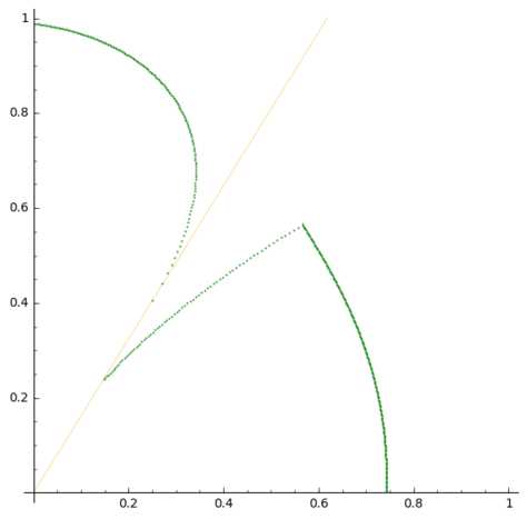
(b) Darga 4, $\text{c\!n}/\text{i\!l}$

Axes: $b$ — horizontal, $c$ — vertical. Black rays are facets of the interlace fan. The polar simplex $\hat{I}^{\ast}$ is yellow; i​l, c​n and b​e are computed on $\hat{I}^{\ast}$ simplex, on each ray. As $\text{i\!l}=1$ on $\hat{I}^{\ast}$, there is a blue circle, while the green curve also represents $\text{c\!n}/\text{i\!l}$ on each ray. The figure on the right is a piece of the green curve.

Figure 1. Darga 4 polynomials

By Proposition 7.1, in $C_{0}$ and $C_{2}$ the polynomials are all exact. We concentrate on $C_{1}$.

Here, the inequality $c>0$ is valid if $p\neq 0$, and we will scale $p$ so that $c=1$, that is $p(x)=bx^{3}+2x^{2}+bx$; as a bonus, $\text{i\!l}\!\mspace{-2.0mu}\left(p\right)=I_{1}(p)=1$. Also, the defining inequalities of $C_{1}$ can be abridged as $|b|\leq 2$.

In order to compute $\text{c\!n}\!\mspace{-2.0mu}\left(p\right)$ and $\text{b\!e}\!\mspace{-1.5mu}\left(p\right)$, we use Theorem 6.13. Up to a constant factor, $H\left(S_{1}\left(p_{\alpha}\right)\right)=(\alpha+b+c)*x^{2}+(-6*\alpha+2*c)*x+\alpha-b+c$, its discriminant (ditto) is $8*\alpha^{2}-8*\alpha+b^{2}$, and $\text{c\!n}\!\mspace{-2.0mu}\left(p\right)$ is the largest of

$$r_{1}=-b-1,\quad r_{2}=b-1,\quad r_{3}={\scriptstyle\frac{1+\sqrt{1-\frac{1}{2}b^{2}}}{2}}.$$

More simply, $\text{c\!n}\!\mspace{-2.0mu}\left(p\right)=\max\{|b|-1,r_{3}\}$, where $r_{3}$ is only considered for $|b|\leq\sqrt{2}/2$.

Since $|b|\leq 2$, there are two separate cases:

1. $|b|\leq\sqrt{2}$. Since $|b|-1\leq\sqrt{2}-1<\frac{1}{2}<r_{3}$, $\text{c\!n}\!\mspace{-2.0mu}\left(p\right)=r_{3}$. It follows that $\text{b\!e}\!\mspace{-1.5mu}\left(p\right)=\frac{2}{\scriptstyle\left(1+\sqrt{1-\frac{\text{\phantom{i}}b^{2}}{2}}\right)}-1\leq 1$, and the bound is attained for $b=\pm\sqrt{2}$. Also, in this interval there is a single exact polynomial, specified by $b=0$, namely $p(x)=2x^{2}$.

2. $\sqrt{2}<|b|\leq 2$. In this case, there is no $r_{3}$ to consider, so $\text{c\!n}\!\mspace{-2.0mu}\left(p\right)=|b|-1$, and $\text{b\!e}\!\mspace{-1.5mu}\left(p\right)=\frac{1}{|b|-1}-1<\sqrt{2}$. As $|b|\rightarrow\sqrt{2}$, $\text{c\!n}\!\mspace{-2.0mu}\left(p\right)\rightarrow\sqrt{2}-1$ and $\text{b\!e}\!\mspace{-1.5mu}\left(p\right)\rightarrow\sqrt{2}$, but not attained.

The previous paragraphs show that c​n and b​e, are discontinuous at the rays $b=\pm\sqrt{2}c$, and this is illustrated in Fig. 1(b).

It follows that $\text{BE}(4)=\sqrt{2}$.

8.4. Darga 5

The general form is $p(x)=b\sigma\!_{5,1}+c\sigma\!_{5,2}$.

It is well known that $\cos\frac{2\pi}{5}=\frac{\sqrt{5}-1}{4}$, and $\cos\frac{4\pi}{5}=\frac{-\sqrt{5}-1}{4}$. So, from Eq. 15, defining $\gamma=\frac{3+\sqrt{5}}{2}$, we find that the interlace fan comprises the cones:

$$\begin{array}[]{l@{\,}r@{\,}r@{\;}l}C_{0}\!\!:&-b-\gamma c\geq 0,&-\gamma b-c\geq 0,&\text{on which}\ \text{i\!l}\!\mspace{-2.0mu}\left(p\right)=-(b+c).\\ C_{1}\!\!:&b+\gamma c\geq 0,&-b+c\geq 0,&\text{on which}\ \text{i\!l}\!\mspace{-2.0mu}\left(p\right)=\left((b+c)+\sqrt{5}(c-b)\right)/4.\\ C_{2}\!\!:&\gamma b+c\geq 0,&b-c\geq 0,&\text{on which}\ \text{i\!l}\!\mspace{-2.0mu}\left(p\right)=\left((b+c)+\sqrt{5}(b-c)\right)/4.\end{array}$$

In order to compute $\text{c\!n}\!\mspace{-2.0mu}\left(p\right)$ and $\text{b\!e}\!\mspace{-1.5mu}\left(p\right)$, we use Theorem 6.13. Up to a constant factor, $H\left(S_{1}\left(\frac{p_{\alpha}}{x+1}\right)\right)=(\alpha+b+c)x^{2}+(-10\alpha-2b+2c)x+5\alpha-3b+c$, its discriminant (ditto) is $5\alpha^{2}-(4c-2b)\alpha+b^{2}$, and $\text{c\!n}\!\mspace{-2.0mu}\left(p\right)$ is the largest of

$$r_{1}=-b-c,\quad r_{2}=\frac{3b-c}{5},\quad r_{3}=\frac{1}{5}\left(2c-b+2\sqrt{c^{2}-bc-b^{2}}\right),$$

where $r_{3}$ can only contribute to the circle number if $c^{2}-bc-b^{2}\geq 0$.

We analyze each cone separately:

$C_{0}:$ Here all polynomials are exact, so there is nothing interesting to be said.

$C_{2}:$ Here, $b>0$ is a valid inequality for all nonzero polynomials, so we scale, making $b=1$. Hence, we have $p(x)=\sigma\!_{5,1}+c\sigma\!_{5,2}$, $-\frac{3+\sqrt{5}}{2}\leq c\leq 1$, and $\text{i\!l}\!\mspace{-2.0mu}\left(p\right)=\frac{1}{4}\left((1-\sqrt{5})c+1+\sqrt{5}\right)$. Also, $r_{3}$ exists either for $c\geq(1+\sqrt{5})/2$, which is out of $C_{2}$, or for $c\leq(1-\sqrt{5})/2$, on which $r_{3}<0$. So, it turns out that $\text{c\!n}\!\mspace{-2.0mu}\left(p\right)=\max\{r_{1},r_{2}\}$. Each of them can be the largest, so we have:

$$\text{c\!n}\!\mspace{-2.0mu}\left(p\right)=\begin{cases}{\scriptstyle-1-c}&\text{if}\quad\;\,c\leq-2\\ \phantom{.}\frac{3-c}{5}&\text{if}\ -2\leq\phantom{-}c,\end{cases}$$

and it happens to be continuous. Computing $\text{b\!e}\!\mspace{-1.5mu}\left(p\right)$ in each case, we find that its maximum in $C_{2}$ is attained at $c=-2$ and its value is $\frac{3\sqrt{5}-5}{4}\cdot$

$C_{1}:$ Here, $c>0$ is a valid inequality for all nonzero polynomials, so we scale, making $=1$. Hence, we have $p(x)=b\sigma\!_{5,1}+\sigma\!_{5,2}$, $-\frac{3+\sqrt{5}}{2}\leq b\leq 1$, and $\text{i\!l}\!\mspace{-2.0mu}\left(p\right)=\frac{1}{4}((1-\sqrt{5})b+1+\sqrt{5})$. There exists an $r_{3}$ in the interval $\left[-\frac{3+\sqrt{5}}{2},-\frac{1+\sqrt{5}}{2}\right]$, and this splits the interval $[-({3+\sqrt{5}})/{2},1]$ into three parts, as follows:

• $-\frac{3+\sqrt{5}}{2}\leq b<-\frac{1+\sqrt{5}}{2}$: $r_{1}=-b-1$ is the largest root; so, as $b\rightarrow-\frac{1+\sqrt{5}}{2}$, $\text{c\!n}\!\mspace{-2.0mu}\left(p\right)\rightarrow\frac{\sqrt{5}-1}{2}$ and $\text{b\!e}\rightarrow\sqrt{5}+1$; further, b​e is increasing and bounded above by the value shown.

• $-\frac{1+\sqrt{5}}{2}\leq b\leq\frac{\sqrt{5}-1}{2}$: in this interval $r_{3}$ exists, and it is the largest root. Note that for $b=-\frac{1+\sqrt{5}}{2}$, $\text{c\!n}\!\mspace{-2.0mu}\left(p\right)=\frac{5+\sqrt{5}}{10}$ and $\text{b\!e}\!\mspace{-1.5mu}\left(p\right)=\frac{1+\sqrt{5}}{4}$; for $b=\frac{\sqrt{5}-1}{2}$, $\text{c\!n}\!\mspace{-2.0mu}\left(p\right)=\frac{5-\sqrt{5}}{10}$ and $\text{b\!e}\!\mspace{-1.5mu}\left(p\right)=\sqrt{5}-1$, which is maximum in the interval.

  Also, in this interval, there exists a single exact polynomial (just find $b$ such that $\text{i\!l}\!\mspace{-2.0mu}\left(p\right)=r_{3}$), specified by $b=\frac{1-\sqrt{5}}{6}$ (see Example 7.1).

• $\frac{\sqrt{5}-1}{2}<b\leq 1$: here $r_{2}=\frac{3b-1}{5}$ is largest; as $b\rightarrow\frac{\sqrt{5}-1}{2}$, $\text{c\!n}\!\mspace{-2.0mu}\left(p\right)\rightarrow\frac{3\sqrt{5}-5}{10}$ and $\text{b\!e}\rightarrow\frac{3+\sqrt{5}}{2}$, which is an upper bound for b​e, but not attained.

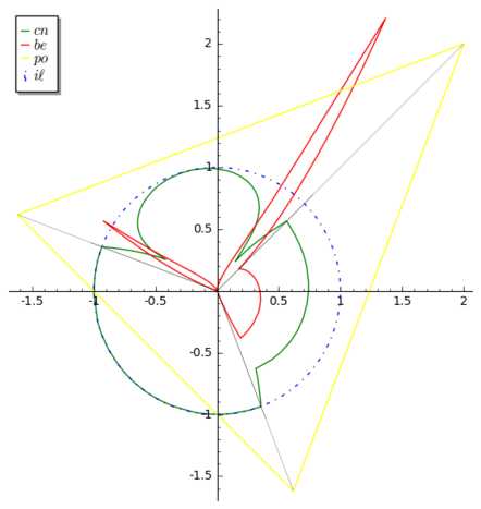
(a) All numbers, darga 5

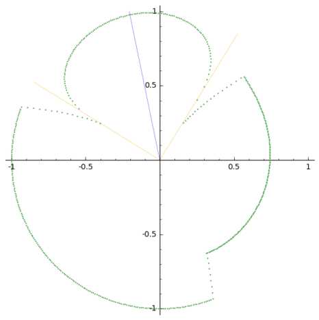
(b) Darga 5, $\text{c\!n}/\text{i\!l}$

Figure 2. Darga 5 polynomials

So, we note that c​n and b​e have two rays of discontinuity, spanned by $\frac{-1\pm\sqrt{5}}{2}\sigma\!_{5,1}+\sigma\!_{5,2}$. Figure 2(a) follows the same conventions as Figure 1(a). Figure 2(b) shows $\text{c\!n}/\text{i\!l}$, along with the fan rays, discontinuity rays and the exceptional exact polynomial.

The whole analysis also implies that $\text{BE}(5)=\frac{3+\sqrt{5}}{2}\cdot$

8.5. Darga 6

The FOIC corresponding to darga 6 has been explicitly described in Example 5.3, and it happens to be a rational cone. Unfortunately, a general study of the circle number seems to be too complicated to be worth it. We just recall our recurring example $p(x)=50x^{5}+86x^{4}+99x^{3}+86x^{2}+50x$, which lies in $C_{1}$ and has bounding error exactly $4$. It would be really nice if it was maximum, but numerical experimentation led to $23p-x^{3}$, whose bounding error yields: $\text{BE}(6)\geq 4.00645161290323$. We also used SageMath and QepCAD [8] to find out about the exact polynomials in cones $C_{1}$ and $C_{2}$, using the characterization in Theorem 7.4. The result was two components on each cone, with rather complicated descriptions.

9. Some interesting families

Here we present some families of polynomials for which something nontrivial can be said about interlace or circle numbers. The first three sections have a number-theoretic flavor, the other ones are more analytic.

9.1. Gcd polynomials

This family of polynomials was the starting point for the research being presented here. [14] studied the following family of polynomials

$$\text{gcd}_{n}^{(k)}(x)=\sum_{j=0}^{n}\gcd(n,j)^{k}x^{j}.$$

At that time, the notions of interlace and circle numbers had not yet come up; the main result there can be stated as

$$\text{i\!l}\!\mspace{-2.0mu}\left(\text{tgcd}_{n}^{(k)}(x)\right)\leq n^{k},$$

where $\text{tgcd}_{n}^{(k)}(x)=\operatorname{trim}{\text{gcd}_{n}^{(k)}(x)}$, but one can extract a more precise result from what is proved there.

Jordan’s totient function is

$$J_{k}(n)=n^{k}\!\!\!\!\prod_{\begin{subarray}{c}p|n\\ p\ \text{prime}\end{subarray}}\left(1-\frac{1}{p^{k}}\right),$$

and, in particular, $J_{1}(n)=\varphi(n)$.

It is stated as Prop.1 of [14] that for every $m$

$$n^{k}+\text{tgcd}_{n}^{(k)}\left(\IfSubStr{m;n}{;}{\text{e}^{\frac{2\pi i\StrBefore{m;n}{;}}{\raisebox{2.0pt}{$\scriptscriptstyle\StrBehind{m;n}{;}$}}}}{\text{e}^{2i\pi m;n}}\right)=\sum_{d|\gcd(m,n)}dJ_{k}\left(\frac{n}{d}\right).$$

It is easy to see that the sum on the right is minimized if $\gcd(m,n)=1$, where its value is simply $J_{k}(n)$. It follows that

(16) $$\text{i\!l}\!\mspace{-2.0mu}\left(\text{tgcd}_{n}^{(k)}(x)\right)=\frac{n^{k}-J_{k}(n)}{2}\mathbin{\raisebox{2.15277pt}{,}}$$

and the interlace certs are precisely the elements of $V_{n}$ that generate the group $U_{n}$. Notice that the interlace number is an integer if $n$ is even. Moreover, this value is generally much smaller than the upper bounds provided in Section 4. Also, if $n$ is prime, $\text{tgcd}_{n}^{(k)}(x)=\operatorname{ge}_{n}(x)$, and indeed Eq. 16 yields the value $\frac{1}{2}$ for the interlace number, as expected. The next result ties in with the following section.

Proposition 9.1.

Let $a(x)=\sum_{k=0}^{m}a_{k}x^{k}$ be a polynomial with nonnegative real coefficients. Then,

$$\text{i\!l}\!\mspace{-2.0mu}\left(\sum_{j=0}^{n}a(\gcd(n,j))x^{j}\right)=\frac{1}{2}\left(a(n)-\sum_{k=0}^{m}a_{k}J_{k}(n)\right).$$

Proof.

First, note that $J_{0}(n)=0$ if $n>1$, and Eq. 16 holds true if $k=0$. Furthermore, $\IfSubStr{;n}{;}{\text{e}^{\frac{2\pi i\StrBefore{;n}{;}}{\raisebox{2.0pt}{$\scriptscriptstyle\StrBehind{;n}{;}$}}}}{\text{e}^{2i\pi;n}}$ is an interlace cert for all $\text{tgcd}_{n}^{(k)}$, so all these polynomials are in the cone $C_{1}$ of the interlace fan. So are all nonnegative linear combinations of those polynomials, and, as the interlace number is linear on $C_{1}$, the result follows from Eq. 16. ∎

We have no idea on how to express $\text{c\!n}\!\mspace{-2.0mu}\left(\text{tgcd}_{n}(x)\right)$, but experiments suggest that $\text{b\!e}\!\mspace{-1.5mu}\left(\text{tgcd}_{n}(x)\right)$ is always positive, and goes to 0 with $n$.

9.2. Interlace rational polynomials

We will use, exclusively in this section, the notation $(r,k)$ to stand for $\gcd(r,k)$; $n$ will be fixed throughout. Recall that for every $1\leq r<n$, ${\theta_{n}\!}^{r}$ is a primitive $\frac{n}{d}$th root of unity, where $d=(r,n)$, and its conjugates over $\mathbb{Q}$ are $\left\{\left.{\theta_{n}\!}^{kd}\,\right|\;(k,n/d)=1\right\}$. We refer to those sets as conjugate classes of roots of unity; these classes can be indexed by the divisors of $n$, the $d$-class being $\left\{\left.{\theta_{n}\!}^{k}\,\right|\;(k,n)=d\right\}$.

The coprime-support polynomials are the stars of this section and are defined as:

$$R_{n}(x)=\sum_{\begin{subarray}{c}0<k<n\\ (k,n)=1\end{subarray}}x^{k}.$$

Clearly, $R_{n}(1)=\varphi(n)$. More generally, for every $j$, $c_{n}(j)=R_{n}({\theta_{n}\!}^{j})$ is called a Ramanujan sum [36]. This is known to be integer, and indeed

(17) $$c_{n}(j)=\mu\left(\frac{n}{(n,j)}\right)\frac{\varphi(n)}{\varphi\left(\frac{n}{(n,j)}\right)}\cdot$$

The following lower bound for the interlace number turns out to be racional if the polynomial has racional coefficients.

Proposition 9.2.

Let $p$ be a darga $n$ trim palindromic polynomial. Then,

(18) $$\text{i\!l}\!\mspace{-2.0mu}\left(p\right)\geq\max_{d|n}\frac{-1}{\varphi(d)}\sum_{j=1}^{\lfloor n/2\rfloor}\tilde{p}_{j}c_{d}(j).$$

Proof.

We know, by the Interlace Formula, that $\text{i\!l}\!\mspace{-2.0mu}\left(p\right)\geq-\frac{1}{2}p(\omega)$ for every $\omega\in U_{n}$. For each $d$, consider the class of primitive $d$-roots of unity; averaging those inequalities over the class gives $-\frac{1}{2\varphi(d)}\sum_{j=1}^{n-1}p_{j}c_{d}(j)$. Noticing that $c_{d}(n-j)=c_{d}(j)$, the last step (to the $\sigma\!$-representation) follows. ∎

A trim palindromic polynomial with rational coefficients will be said to be interlace rational provided its interlace number is rational. If such a polynomial has integer $\sigma\!$-coefficients, $\text{i\!l}\!\mspace{-2.0mu}\left(p\right)$ is an algebraic integer, hence, an integer. Clearly, any rational polynomial in $C_{0}$ or $C_{n/2}$ is interlace rational. More generally:

Proposition 9.3.

If $p$ is interlace rational of darga $n$, then the set of interlace certs of $p$ is a union of conjugate classes. Furthermore,

(19) $$\text{i\!l}\!\mspace{-2.0mu}\left(p\right)=\max_{d|n}\frac{-1}{\varphi(d)}\sum_{j=1}^{\lfloor n/2\rfloor}\tilde{p}_{j}c_{d}(j).$$

Proof.

Lemma 9.4 implies that if $\omega$ is an interlace cert, so are all its conjugates. Proposition 9.2 tells us that the right hand side is a lower bound. Now, choose $d|n$ such that $\text{i\!l}\!\mspace{-2.0mu}\left(p\right)=-\frac{1}{2}p({\theta_{n}\!}^{n/d})$ and apply Eq. 20 to see that it is attained. ∎

Lemma 9.4.

Let $p$ be a polynomial of with rational coefficients. If for some $r$, $p({\theta_{n}\!}^{r})\in\mathbb{Q}$, then $p({\theta_{n}\!}^{kd})=p({\theta_{n}\!}^{r})$ for all $k$ such that $(k,n/d)=1$, where $d=(n,r)$. Moreover,

(20) $$p({\theta_{n}\!}^{d})=\frac{1}{\varphi\left(n/d\right)}\sum_{j}p_{j}c_{n/d}(j).$$

Proof.

Since ${\theta_{n}\!}^{r}$ is a root of $p(x)-p({\theta_{n}\!}^{r})$, so are all its conjugates, hence $p(\omega)=p({\theta_{n}\!}^{d})$ for all $\omega$ in the conjugate class of ${\theta_{n}\!}^{d}$. Averaging this equation over the conjugate class, we get Eq. 20. ∎

Coprime-support polynomials afford a simple formula for the interlace number:

Proposition 9.5.

Let $q$ be the smallest prime factor of $n$. Then $\text{i\!l}\!\mspace{-2.0mu}\left(R_{n}\right)=\frac{\varphi(n)}{2(q-1)}=\frac{R_{n}(1)}{2(q-1)}$, and its interlace certs are the primitive $q$-roots of unity.

Proof.

From the Interlace Formula, $\text{i\!l}\!\mspace{-2.0mu}\left(R_{n}\right)\!=\!-\frac{1}{2}\min_{j}c_{n}(j)\!=\!-\frac{1}{2}\min_{j|n}c_{n}(j)$. The last equality follows from Eq. 17, which implies $c_{n}(j)=c_{n}((n,j))$, so the values of $c_{n}$ are attained at divisors of $n$. If $j$ is such that $c_{n}(j)$ is minimum, one must have $\mu(n/j)=-1$, so $n/j$ is a product of an odd number of distinct primes; also, $\varphi(n/j)$ must be minimum. Those two conditions imply that $n/j=q$, and the result follows from the fact that $\varphi(q)=q-1$, and that the interlace certs are the proper powers of ${\theta_{n}\!}^{j}$. ∎

Here, again, $n$ prime get us back to the geometric polynomial, with the expected result.

Let $p$ be a trim darga $n$ polynomial. Trivially,

$$p(x)=\sum_{d|n}\sum_{\begin{subarray}{c}d\leq j<n\\ (j,n)=d\end{subarray}}p_{j}x^{j}=\sum_{d|n}\sum_{\begin{subarray}{c}1\leq j<n/d\\ (j,n/d)=1\end{subarray}}p_{jd}x^{jd}.$$

An arithmetic function $f:\mathbb{N}\rightarrow\mathbb{C}$ is said to be $n$-even ([36],[38]) if for all $j$, $f(j)=f((j,n))$. We attach the same name to polynomials $p$ of degree $\leq n$ such that for all $j$, $p_{j}=p_{(j,n)}$. Then, we can write

(21) $$p(x) =\sum_{d|n}\>p_{d}\!\!\!\!\sum_{\begin{subarray}{c}d\leq j<n\\ (j,n)=d\end{subarray}}x^{j}$$

(22) $$=\sum_{d|n}\>p_{d}\!\!\!\!\!\sum_{\begin{subarray}{c}1\leq j<n/d\\ (j,n/d)=1\end{subarray}}x^{jd}$$

(23) $$=\sum_{d|n}p_{d}R_{n/d}(x^{d}).$$

So, for every $k$,

(24) $$p({\theta_{n}\!}^{k})=\sum_{d|n}p_{d}c_{n/d}(k),$$

which is the main result in [35].

It follows from Theorem 4.2 and Eq. 24 that rational $n$-even polynomials are interlace rational. The converse is not true. On one hand, $n$-even polynomials lie in a rational linear subspace of dimension equal to the number of divisors of $n$; on the other hand, $C_{0}$ and $C_{n/2}$ are $\left\lfloor n/2\right\rfloor$-dimensional cones whose rational points are all interlace rational. However, those cones are quite special, and Proposition 9.3 restricts the faces of the FOIC that contain interlace rational polynomials. We show next how to construct some of those polynomials in thinner faces.

Example 9.1:

Let $n$ be an odd number and $q$ be its smallest prime factor. Let $g$ be any rational darga $n/q$ trim palindromic polynomial such that $q(1)=0$. Consider now $p(x)=R_{n}(x)+\lambda g(x^{q})$, where $\lambda$ is a positive rational. Proposition 9.5 tells us that any primitive $q$-root of unity $\omega$ is an interlace cert for $R_{n}(x)$. The choice of $g$ implies that $p(\omega)=R_{n}(\omega)$, and with $\lambda$ small enough we can guarantee that $p(\omega)=\min_{r}p({\theta_{n}\!}^{r})$, so it follows that $\text{i\!l}\!\mspace{-2.0mu}\left(p\right)=\text{i\!l}\!\mspace{-2.0mu}\left(R_{n}\right)$, with the same interlace certs. For concreteness, choose an odd prime $q$ and an integer $n$ such that $q$ is the smallest prime factor of $qn$ and let $p(x)=R_{qn}(x)+\sigma\!_{n,1}(x^{q})-\sigma\!_{n,2}(x^{q})$. One can show (exercise for the reader) that, provided $\varphi(n)-\varphi(q)\geq 4$, $p(x)$ is interlace rational; also, the same construction, but violating the inequality, yields polynomials which are not interlace rational.

A further consequence of Eq. 24 is that if the coefficients of $p$ are integers, so are the coefficients of $\hat{p}$, hence $2\text{i\!l}\!\mspace{-2.0mu}\left(p\right)$ is an integer.

Example 9.2:

The geometric polynomial is is trivially $n$-even, and $\operatorname{ge}_{n}(x)=\sum_{d|n}R_{n/d}(x^{d})$. It follows that

$$R_{n}(x)=\sum_{d|n}\mu(d)\operatorname{ge}_{n/d}(x^{d}).$$

Example 9.3:

The trimmed gcd polynomials are $n$-even, and can be simply written as

$$\text{tgcd}_{n}^{(k)}(x)=\sum_{d|n}d^{k}R_{n/d}(x^{d}).$$

Example 9.4:

Suppose $n=q^{m}$, with $q$ prime, and that $p$ is $n$-even; write $a_{j}=p_{q^{j}}$. Then from Eq. 23

$$p(x)=\sum_{j=1}^{m}a_{j}R_{q^{m-j}}(x^{q^{j}}).$$

From Proposition 9.5, $\text{i\!l}\!\mspace{-2.0mu}\left(R_{n}\right)=\frac{1}{2}q^{m-1}$, and its interlace certs are the $q$-th roots of unity. Exponent scaling implies that $\text{i\!l}\!\mspace{-2.0mu}\left(R_{q^{m-j}}(x^{q^{j}})\right)\!=\frac{1}{2}q^{m-j-1}$, and, further, the $q$-th roots of unity are also interlace certs of all those polynomials. Hence the polynomials are all in the face of the interlace fan corresponding to all those roots, so that, provided the $a_{j}$ are nonnegative,

$$\text{i\!l}\!\mspace{-2.0mu}\left(p\right)=\frac{1}{2}\sum_{j=1}^{m}a_{j}q^{m-j-1}.$$

Example 9.5:

This is a more general form of the previous example. Start with a positive integer $n$, and denote by $q$ its smallest prime divisor. Let reals $a_{d}\geq 0$ be given for every $d$ such that $q|d$ and $d|n$. Then, if $p(x)=\sum_{q|d|n}a_{d}R_{\frac{n}{d}}(x^{d})$, its interlace number is $\text{i\!l}\!\mspace{-2.0mu}\left(p\right)=\frac{1}{2(q-1)}p(1)$.

Given the special role of the coprime-support polynomials, one are tempted to ask about their circle number. Half of the task is easy: if $n$ is even, $R_{n}(x)$ is an odd polynomial, so $-1$ is an interlace cert and $p$ is exact, with $\text{c\!n}\!\mspace{-2.0mu}\left(p\right)=\text{i\!l}\!\mspace{-2.0mu}\left(p\right)=\frac{\varphi(n)}{2}\cdot$ The other half we cannot do, and is left to the reader. Computations up to $n=40$ suggest that $\text{b\!e}\!\mspace{-1.5mu}\left(R_{n}\right)$ is positive, but vanishingly small.

9.3. Fekete polynomials

For prime $n$, $n$-even polynomials are just geometric polynomials and give us nothing new. Fekete polynomials are interesting examples of prime degree polynomials whose interlace number and certs have a nice description; they are defined by

(25) $$f_{n}(x):=\sum_{j=1}^{n-1}\left(\frac{j}{n}\right)x^{j},$$

for each prime $n$, and we note that the darga of $f_{n}(x)$ is equal to $n$. Here $\left(\frac{j}{n}\right)$ is the usual Legendre symbol, defined to be equal to $+1$ when $j$ is a quadratic residue mod $n$, and $-1$ when $j$ is a non-quadratic residue mod $n$. We recall that Gauss proved (in his 1811 paper) the following closed form for the Gauss sum, which is by definition equal to $f_{n}(\IfSubStr{k;n}{;}{\text{e}^{\frac{2\pi i\StrBefore{k;n}{;}}{\raisebox{2.0pt}{$\scriptscriptstyle\StrBehind{k;n}{;}$}}}}{\text{e}^{2i\pi k;n}})$

(26) $$f_{n}(\IfSubStr{k;n}{;}{\text{e}^{\frac{2\pi i\StrBefore{k;n}{;}}{\raisebox{2.0pt}{$\scriptscriptstyle\StrBehind{k;n}{;}$}}}}{\text{e}^{2i\pi k;n}})=\epsilon_{n}\sqrt{n}\left(\frac{k}{n}\right),$$

for all $k=0,1,2,\dots,n-1$, where

$$\epsilon_{n}:=\begin{cases}1,\text{ if }n\equiv 1\text{ mod }4,\\ i,\text{ if }n\equiv 3\text{ mod }4.\end{cases}$$

The polynomials $f_{n}(x)$ are trim, palindromic polynomials provided $n\equiv 1\mod 4$. In that case, it follows from (26) that $\left|f_{n}(x)\left(\IfSubStr{k;n}{;}{\text{e}^{\frac{2\pi i\StrBefore{k;n}{;}}{\raisebox{2.0pt}{$\scriptscriptstyle\StrBehind{k;n}{;}$}}}}{\text{e}^{2i\pi k;n}}\right)\right|=\sqrt{n}$, for all $k=0,1,\dots,n-1$, and we may therefore read from the latter identity the interlace number of the Fekete polynomials, by using the Interlace Formula:

(27) $$\text{i\!l}\!\mspace{-2.0mu}\left(f_{n}(x)\right)=\frac{\sqrt{n}}{2}\cdot$$

It follows from Proposition 5.5 that, as every primitive $n$th root of unity is a cert for $f_{n}(x)$, it lives in the same face of the FOIC as $\text{tgcd}_{n}(x)$.

9.4. Half monotonic polynomials

Consider a trim palindromic polynomial $p$ of darga $n$. If the sequence $p_{1},p_{2},\ldots,p_{\left\lfloor n/2\right\rfloor}$ is monotonic, increasing or decreasing, we say that the polynomial is half monotonic, increasing or decreasing, respectively, and strictly so if all those coefficients are distinct.

Proposition 9.6.

If $p$ is strictly increasing, then

$$\text{i\!l}\!\mspace{-2.0mu}\left(p\right)\leq\frac{1}{2}p(1)-2\sum_{j=1}^{\lfloor n/4\rfloor-1}p_{j}-c(n)p_{\left\lfloor\frac{n}{4}\right\rfloor},$$

where $c(n)=1,2,2,3$ according to $n$ being $\equiv 0,1,2,3\mod 4$.

Proof.

We refer to Corollary 4.8, and notice that $m(p)=p_{\left\lfloor\frac{n}{4}\right\rfloor}$, $|M|=\left\lfloor\frac{n}{4}\right\rfloor-1$. Hence,

$$\text{i\!l}\!\mspace{-2.0mu}\left(p\right)\leq\frac{1}{2}p(1)-2\sum_{j=1}^{\lfloor n/4\rfloor-1}p_{j}-\left(\left\lfloor\frac{n-1}{2}\right\rfloor-2\left\lfloor\frac{n}{4}\right\rfloor+2\right)p_{\left\lfloor\frac{n}{4}\right\rfloor}.$$

The result now follows from a case analysis. ∎

A theorem of [10], extended by [18, Theorem 7 ], can be stated as:

Theorem 9.7.

If $p$ is decreasing and has nonnegative coefficients, then $cn(p)\leq p_{1}$.

A natural conjecture was that actually $\text{i\!l}\!\mspace{-2.0mu}\left(p\right)\leq p_{1}$, at least when the coefficients are nonnegative. Alas, this is false, in general. A brute force search using SageMath produced several counterexamples. Here are two examples, of odd and even dargas:

$$15x^{8}+14x^{7}+12x^{6}+2x^{5}+2x^{4}+12x^{3}+14x^{2}+15x,$$

$$80x^{9}+75x^{8}+73x^{7}+11x^{6}+2x^{5}+11x^{4}+73x^{3}+75x^{2}+80x.$$

For the first one, the interlace number is $15.018885\ldots$ and the circle number is $\frac{23}{3}$; for the second one, the values are $90.6139\ldots$ and $68$.

In spite of these examples, there is something positive that can be said. Proposition 5.10 implies that if $p_{1}$ is sufficiently larger than the remaining coefficients, $\text{i\!l}\!\mspace{-2.0mu}\left(p\right)=-\frac{1}{2}p(-1)<\frac{1}{2}p_{1}$.

In Joyner’s article [18], the author asks about nonnegative increasing polynomials; that is, for which values of $\alpha\in[0,p_{1}]$ $p_{\alpha}$ is circle rooted.

We do not expect the concepts of circle and interlace number to be of help here. Experiments show that $\text{c\!n}\!\mspace{-2.0mu}\left(p\right)$ is much larger than $p_{1}$, and we can actually prove that for $\text{i\!l}\!\mspace{-2.0mu}\left(p\right)$:

Proposition 9.8.

Suppose that $p\in\mathscr{T}^{(n)}$ is monotonic increasing, and let $m=\lfloor\frac{n}{2}\rfloor$. Then

$$\text{i\!l}\!\mspace{-2.0mu}\left(p\right)\geq \;\tilde{p}_{m}+(\tilde{p}_{m-1}-\tilde{p}_{1})(1-5m^{-2}) \text{if $n$ is even},$$

$$\text{i\!l}\!\mspace{-2.0mu}\left(p\right)\geq \;(\tilde{p}_{m}-\tilde{p}_{1})(1-5n^{-2}) \text{if $n$ is odd}.$$

Proof.

Let us write $s_{j}=\sum_{k=1}^{m}-\tilde{p}_{k}\cos\frac{2\pi jk}{n}$, for $j=0,1,\ldots,m$. The Interlace Formula says that $\text{i\!l}\!\mspace{-2.0mu}\left(p\right)=\max_{j}s_{j}$, so, for any $j$, $\text{i\!l}\!\mspace{-2.0mu}\left(p\right)\geq s_{j}$. We will compute lower bounds for $s_{1}$.

Case 1: $n=2m$ is even. We can rewrite $s_{1}=\sum_{k=1}^{m}-\tilde{p}_{k}\cos\frac{\pi k}{m}$. Noticing that $\cos\frac{\pi k}{m}=-\cos\frac{\pi(m-k)}{m}$ is positive for $k\leq\frac{m}{2}$, we can rewrite: $s_{1}=\tilde{p}_{m}+\sum_{1\leq k\leq\frac{m}{2}}(\tilde{p}_{m-k}-\tilde{p}_{k})\cos\frac{\pi k}{m}$, and, since $p$ is increasing, all terms in the sum are nonnegative. So, $s_{1}\geq\tilde{p}_{m}+(\tilde{p}_{m-1}-\tilde{p}_{1})\cos\frac{\pi}{m}$. From the Taylor series, $\cos x\geq 1-x^{2}/2$, so $\cos\frac{\pi}{m}\geq 1-\pi^{2}/{2m^{2}}\geq 1-5/m^{2}$, and this case is done.

Case 2: $n=2m+1$ is odd. Notice that for $1\leq k\leq\frac{m}{2}$ we have
$\cos 2\pi(m-k+1)/n\leq 0$ , and $-\cos 2\pi(m-k+1)/n\geq\cos 2\pi k/n$. Rewrite $s_{1}=\sum_{1\leq k\leq\frac{m}{2}}\big{(}-\tilde{p}_{m-k+1}\cos 2\pi(m-k+1)/n-\tilde{p}_{k}\cos 2\pi k/n\big{)}$ (actually, if $m$ is odd, there is an additional negative term). Using the inequalities on cosines at the beginning of the paragraph, we can bound $s_{1}\geq\sum_{1\leq k\leq\frac{m}{2}}(\tilde{p}_{m-k+1}-\tilde{p}_{k})(-\cos 2\pi(m-k+1)/n)$, and, as all summands are nonnegative, we can bound $s_{1}\geq(\tilde{p}_{m}-\tilde{p}_{1})\cos 2\pi/n$. We bound $\cos 2\pi/n$ as in Case 1 to get the result. ∎

9.5. Binomial polynomials

An interesting case study of half-monotonic increasing polynomial is that of $B_{n}(x)=(1+x)^{n}-(1+x^{n})$, trimmed binomial polynomials, which will also be relevant in the next subsection. Here we can calculate the exact value

(28) $$\text{i\!l}\!\mspace{-2.0mu}\left(B_{n}\right)=2^{n-1}\cos^{n}\frac{\pi}{n}-1.$$

Since $\cos\frac{\pi}{n}=1-O(1/n^{2})$, we have the asymptotics $\text{i\!l}\!\mspace{-2.0mu}\left(B_{n}\right)=2^{n-1}(1-O(1/n))$.

Proof of (28).

We show that $\min_{\omega\in V_{n}}(1+\omega)^{n}=-(2\cos\frac{\pi}{n})^{n}$, and then apply the Interlace Formula. Let $\omega\in V_{n}\backslash\{1\}$, and let $\zeta\in V_{2n}$ be such that $\zeta^{2}=\omega$. Then, $(1+\omega)^{n}=(1+\zeta^{2})^{n}=2^{n}\zeta^{n}\Re(\zeta)^{n}$. Since $\zeta^{n}=\pm 1$, the last value is minimized at $\zeta=\IfSubStr{;n}{;}{\text{e}^{\frac{2\pi i\StrBefore{;n}{;}}{\raisebox{2.0pt}{$\scriptscriptstyle\StrBehind{;n}{;}$}}}}{\text{e}^{2i\pi;n}}$, as $\zeta^{n}=-1$ and it has the largest real part, attaining the value $-2^{n}\cos^{n}\frac{\pi}{n}\cdot$ ∎

Computation up to $n=40$ suggests that $\text{c\!n}\!\mspace{-2.0mu}\left(B_{n}\right)$ is just above $2^{n-1}\cos^{n+3}\frac{\pi}{n}$, so $\text{b\!e}\!\mspace{-1.5mu}\left(B_{n}\right)<\frac{1}{\cos^{3}\frac{\pi}{n}}-1=O(\frac{1}{n^{2}})$.

The “Hadamard inverse” $B_{n}^{H}=\sum_{k=1}^{n-1}\binom{n}{k}^{-1}x^{k}$ is decreasing, so we have some information provided at the previous section; actually, a much more precise results follow from Proposition 5.10. Writing $p_{k}=\binom{n}{k}^{-1}$, one can show that for $k\geq 3$, $k^{2}\tilde{p}_{k}<3^{2}\tilde{p}_{3}$; one way to verify this is to note that $(k-1)^{2}\tilde{p}_{k-1}<k^{2}\tilde{p}_{k}$ for $k\leq n/2$ (the case $k=n/2$ requires special attention). Now,

(29) $$\tilde{p}_{1}-\sum_{k=2}^{\left\lfloor n/2\right\rfloor}k^{2}|\tilde{p}_{k}| \geq p_{1}-4p_{2}-(\left\lfloor n/2\right\rfloor-2)\cdot 3^{2}p_{3}$$

(30) $$=\frac{1}{n}-\frac{8}{n(n-1)}-\frac{27(n-4)}{n(n-1)(n-2)}$$

(31) $$\geq\frac{1}{n}\left(1-\frac{35}{n-1}\right)$$

and this is positive if $n\geq 36$. So, by Proposition 5.10, for those $n$, $-1$ is an interlace cert of $B_{n}^{H}$ if $n$ is even, so $B_{n}^{H}$ is exact. For $n$ odd, ${\theta_{n}\!}^{\left\lfloor n/2\right\rfloor}$ is an interlace cert and it looks like $-1$ is a circle cert. Computer verification extends the same conclusions to $2\leq n\leq 35$. Curiously, the expression on the left of Eq. 29 is negative for $6\leq n\leq 17$, so Proposition 5.10 cannot be applied to handle these cases.

9.6. Cut polynomials

Let $A$ be an $n\times n$ Hermitian matrix, define its cut polynomial (see [2]) by

$$\text{Cut}_{A}(x)=\sum_{S\subseteq\{1,\ldots,n\}}x^{|S|}\prod_{\begin{subarray}{c}i\in S\\ j\not\in S\end{subarray}}a_{ij},$$

and let $\text{TCut}_{A}(x)=\operatorname{trim}\text{Cut}_{A}(x)$.

The celebrated Lee-Yang Theorem [28] states that

if $|a_{ij}|\leq 1$ for all $i,j$, then $\text{Cut}_{A}(x)$ is circle rooted.

One easily sees that the cut polynomial is self-inversive, hence the question comes to mind as whether the Lee-Yang Theorem has any relation to either interlace number or circle number.

The answer is, nothing much, in general. Consider, for instance, the matrix $J$ of all 1’s. It is easy to see that $\text{Cut}_{J}(x)=(1+x)^{n}$, so $\text{TCut}_{J}(x)=B_{n}(x$). As we have seen, both $\text{i\!l}\!\mspace{-2.0mu}\left(B_{n}\right)$ and $\text{c\!n}\!\mspace{-2.0mu}\left(B_{n}\right)$ are very large, and say nothing about the monic cut polynomial.

But all is not lost. Suppose we restrict a little the set of matrices, requiring that all $|a_{ij}|\leq\lambda$, for some $0<\lambda(n)<1$. Then, each product in the definition of $\text{Cut}_{A}(x)$ has absolute value at most $\lambda^{k(n-k)}$, where $k=|S|$, and we can apply Theorem 4.6 to conclude that

$$\text{i\!l}\!\mspace{-2.0mu}\left(\text{TCut}_{A}\right)\leq\frac{1}{2}\sum_{k=1}^{n-1}\binom{n}{k}\lambda^{k(n-k)}\leq\sum_{k=1}^{\lfloor n/2\rfloor}\binom{n}{k}\lambda^{k(n-k)}$$

Denote $LY(x)=\sum_{k=1}^{\lfloor n/2\rfloor}\binom{n}{k}x^{k(n-k)}$; if $LY(\lambda)\leq 1$, then it follows that $\text{Cut}_{A}(x)$ angle interlaces $U_{n}$, so in this case we have a stronger conclusion than in Lee-Yang. For $n>2$, $LY(1)>0$, $LY(0)=-1$, and $LY(x)$ is increasing for positive $x$. So, the best possible value for $\lambda$ is the only positive root of $LY(x)-1$, which probably does not have a neat closed form.

Let us show that $\lambda=1/(cen)^{2/n}$ is a lower bound for the root, for some $c>1$.

Indeed, for $1\leq k\leq n/2$,

$$\binom{n}{k}\lambda^{k(n-k)}\leq\binom{n}{k}\lambda^{kn/2}\leq\left(\frac{ne}{k}\right)^{k}(cen)^{-k}=\frac{1}{c^{k}k^{k}}\cdot$$

Hence, $LY(\lambda)\leq\sum_{k\geq 1}\frac{1}{(ck)^{k}}\leq\frac{1}{c}\sum_{k\geq 1}\frac{1}{k^{k}}\leq\frac{1}{c}\sum_{k\geq 1}\frac{1}{4^{k-1}}\leq 1$ for $c\geq 4/3$ (although $5/4$ seems to be more accurate); that is, $\lambda=\text{e}^{-2\frac{\log n}{n}-h}$, where $h$ is a constant, slightly larger than 1.

Anyway, we have shown that $\text{i\!l}\!\mspace{-2.0mu}\left(\text{TCut}_{A}\right)\leq 1$ if $|a_{ij}|\leq\text{e}^{-2\frac{\log n}{n}-h}$. The actual root of $LY(x)-1$ seems to grow as $\text{e}^{-\alpha\frac{\log n}{n}}$, where $1<\alpha<2$.

10. Open problems

Here we delve into some open questions that are scattered throughout the paper, and we present future research directions in which we hope more people can join us.

The general theory of the interlace number seems quite satisfactory at this point. The circle number is a different ball game. There is some hope that a concerted attack on the semi-algebraic side will yield new insights. The same comments hold for exact polynomials.

Problem 1.

What is the geometry (maybe just the topology) of the set of exact polynomials, for each darga $\geq 6$? Is it connected? In particular, what happens within each $C_{j}$, where the exact polynomials fall into distinct components; can these polynomials be parameterized?

Problem 2.

What about the growth of $\text{BE}(n)$? We have shown a linear lower bound, and the construction used for it is intuitively (for us) best possible, but we have no proof of that. In Section 8 we have shown that BE(4) and BE(5) are not attained by any polynomial. Does this happen for all larger values of $n$?

Polynomials with rational coefficients give rise to several questions; in most of them, there is no loss of generality in considering only integer polynomials.

Problem 3.

What are the minimal faces of the FOIC that contain rational points? Most rays clearly do not (except in darga 6). On the other hand, Section 9.2 gives several examples of faces that do. Are there interlace rational polynomials in those minimal faces?

Problem 4.

We repeat the same question as above, but for exact polynomials. Outside of the polyhedral cones $C_{0}$ and $C_{n/2}$ in the FOIC, what do exact rational polynomials look like? In Example 7.1, we present a family of exact rational polynomials. Does every component of the set of exact polynomial contain a rational point? Are there interlace rational exact polynomials?

Problem 5.

Proposition 5.10 can be unwound into an inequalities description of a rational cones contained in the cone $C_{n/2}$. Can we get, for each $j$, interesting rational cones contained in $C_{j}$?

Problem 6.

Is there an algorithm involving only rational arithmetic for finding out all the interlace certs of a given rational polynomial, describing them as appropriate powers of $\theta_{n}$ ?

Problem 7.

What are the ranges of i​l, c​n and b​e, computed over integer polynomials? Are all nonnegative real algebraic numbers attainable? For i​l, there is already a restriction: it must belong to a cyclotomic field.

Problem 8.

The gcd polynomials empirically share the following properties: they are never exact, but their bounding error is $O(1/n)$ for darga $n$. In particular, this includes the geometric polynomials of prime darga, for which this is a known fact (Example 7.4). Is it always true?

Problem 9.

A global view of rational polynomials could be provided by the development of Erhart theory for the interlace simplex, and for the cones in the FOIC. That is highly developed and well understood in case of rational polyhedral cones, but little is known for cones that are not rational. The FOIC cones are, in a sense, just shy of being rational, and may be still treatable.

Finally, here is a different type of question, which was already hinted at in Example 6.3:

Problem 10.

Is there a family polynomials $p$ for which the set of values $\alpha$ for which $p_{\alpha}$ is circle rooted fall into increasingly many disjoint intervals?

Glossary

circle-number

for $p$ trim self-inversive,
$\text{c\!n}\!\mspace{-2.0mu}\left(p\right)=\inf\left\{\left.\beta\,\right|\;p_{\alpha}\ \text{is circle rooted for all}\ \alpha\geq\beta\right\}$

References

- [1] I. Area, E. Godoy, R.. Lamblém and A. Sri Ranga “Basic hypergeometric polynomials with zeros on the unit circle” In Appl. Math. Comput. 225, 2013, pp. 622–630 DOI: 10.1016/j.amc.2013.09.060
- [2] Alexander Barvinok “Combinatorics and complexity of partition functions” 30, Algorithms and Combinatorics Springer, Cham, 2016, pp. vi+303 DOI: 10.1007/978-3-319-51829-9
- [3] Saugata Basu, Richard Pollack and Marie-Françoise Roy “Algorithms in real algebraic geometry” 10, Algorithms and Computation in Mathematics Springer-Verlag, Berlin, 2006, pp. x+662
- [4] V. Botta, L.. Marques and M. Meneguette “Palindromic and perturbed polynomials: zeros location” In Acta Math. Hungar. 143.1, 2014, pp. 81–87 DOI: 10.1007/s10474-013-0382-0
- [5] Petter Brändén “Unimodality, log-concavity, real-rootedness and beyond” In Handbook of enumerative combinatorics, Discrete Math. Appl. (Boca Raton) CRC Press, Boca Raton, FL, 2015, pp. 437–483
- [6] Petter Brändén, James Haglund, Mirkó Visontai and David G. Wagner “Proof of the monotone column permanent conjecture” In Notions of positivity and the geometry of polynomials, Trends Math. Birkhäuser/Springer Basel AG, Basel, 2011, pp. 63–78 DOI: 10.1007/978-3-0348-0142-3_5
- [7] David Bremner et al. “Computing symmetry groups of polyhedra” In LMS J. Comput. Math. 17.1, 2014, pp. 565–581 DOI: 10.1112/S1461157014000400
- [8] Christopher W. Brown “QEPCAD B: a program for computing with semi-algebraic sets using CADs” In ACM SIGSAM Bulletin 37, 2002, pp. 97–108
- [9] Winfried Bruns and Joseph Gubeladze “Polytopes, rings, and -theory”, Springer Monographs in Mathematics Springer, Dordrecht, 2009, pp. xiv+461 DOI: 10.1007/b105283
- [10] Weiyu Chen “On the polynomials with all their zeros on the unit circle” In J. Math. Anal. Appl. 190.3, 1995, pp. 714–724 DOI: 10.1006/jmaa.1995.1105
- [11] Maria Chudnovsky and Paul Seymour “The roots of the independence polynomial of a clawfree graph” In J. Combin. Theory Ser. B 97.3, 2007, pp. 350–357 DOI: 10.1016/j.jctb.2006.06.001
- [12] Henri Cohen “A course in computational algebraic number theory” 138, Graduate Texts in Mathematics Springer-Verlag, Berlin, 1993, pp. xii+534 DOI: 10.1007/978-3-662-02945-9
- [13] K. Conrad “Roots on a Circle” URL: http://www.math.uconn.edu/~kconrad/blurbs/galoistheory/numbersoncircle.pdf
- [14] Karl Dilcher and Sinai Robins “Zeros and irreducibility of polynomials with gcd powers as coefficients” In Ramanujan J. 36.1-2, 2015, pp. 227–236 DOI: 10.1007/s11139-014-9579-2
- [15] Günter Ewald “Combinatorial convexity and algebraic geometry” 168, Graduate Texts in Mathematics Springer-Verlag, New York, 1996, pp. xiv+372 DOI: 10.1007/978-1-4612-4044-0
- [16] Steve Fisk “Polynomials, roots, and interlacing” In arXiv Mathematics e-prints, 2006, pp. math/0612833 arXiv:math/0612833 [math.CA]
- [17] Juan B. Gil and Sinai Robins “Hecke operators on rational functions. I” In Forum Math. 17.4, 2005, pp. 519–554 DOI: 10.1515/form.2005.17.4.519
- [18] David Joyner “Zeros of some self-reciprocal polynomials” In Excursions in harmonic analysis. Volume 1, Appl. Numer. Harmon. Anal. Birkhäuser/Springer, New York, 2013, pp. 329–348 DOI: 10.1007/978-0-8176-8376-4_17
- [19] David Joyner and Tony Shaska “Self-inversive polynomials, curves, and codes” In Higher genus curves in mathematical physics and arithmetic geometry 703, Contemp. Math. Amer. Math. Soc., Providence, RI, 2018, pp. 189–208 DOI: 10.1090/conm/703/14138
- [20] David C. Kurtz “A sufficient condition for all the roots of a polynomial to be real” In Amer. Math. Monthly 99.3, 1992, pp. 259–263 DOI: 10.2307/2325063
- [21] D.. Kwon “Reciprocal polynomials with all zeros on the unit circle” In Acta Math. Hungar. 131.3, 2011, pp. 285–294 DOI: 10.1007/s10474-011-0090-6
- [22] Piroska Lakatos and László Losonczi “Circular interlacing with reciprocal polynomials” In Math. Inequal. Appl. 10.4, 2007, pp. 761–769 DOI: 10.7153/mia-10-71
- [23] Piroska Lakatos and László Losonczi “On zeros of reciprocal polynomials of odd degree” In JIPAM. J. Inequal. Pure Appl. Math. 4.3, 2003, pp. Article 60\bibrangessep8 pp. (electronic)
- [24] Piroska Lakatos and László Losonczi “Polynomials with all zeros on the unit circle” In Acta Math. Hungar. 125.4, 2009, pp. 341–356 DOI: 10.1007/s10474-009-9028-7
- [25] Piroska Lakatos and László Losonczi “Self-inversive polynomials whose zeros are on the unit circle” In Publ. Math. Debrecen 65.3-4, 2004, pp. 409–420
- [26] Matilde N. Lalín and Mathew D. Rogers “Variations of the Ramanujan polynomials and remarks on ” In Funct. Approx. Comment. Math. 48.part 1, 2013, pp. 91–111 DOI: 10.7169/facm/2013.48.1.8
- [27] Matilde N. Lalín and C.. Smyth “Unimodularity of zeros of self-inversive polynomials” In Acta Math. Hungar. 138.1-2, 2013, pp. 85–101 DOI: 10.1007/s10474-012-0225-4
- [28] T.. Lee and C.. Yang “Statistical theory of equations of state and phase transitions. II. Lattice gas and Ising model” In Physical Rev. (2) 87, 1952, pp. 410–419
- [29] Arnaldo Mandel “Large finite products of small fractions” In arXiv e-prints, 2019, pp. arXiv:1908.00839 arXiv:1902.04231 [math.CA]
- [30] Morris Marden “Geometry of polynomials”, Second edition. Mathematical Surveys, No. 3 American Mathematical Society, Providence, R.I., 1966, pp. xiii+243
- [31] Kathleen L. Petersen and Christopher D. Sinclair “Conjugate reciprocal polynomials with all roots on the unit circle” In Canad. J. Math. 60.5, 2008, pp. 1149–1167 DOI: 10.4153/CJM-2008-050-8
- [32] Q.. Rahman and G. Schmeisser “Analytic theory of polynomials” 26, London Mathematical Society Monographs. New Series The Clarendon Press, Oxford University Press, Oxford, 2002, pp. xiv+742
- [33] The Sage Developers “SageMath, the Sage Mathematics Software System (Version 8.2)” http://www.sagemath.org, 2018
- [34] Carla D. Savage and Mirkó Visontai “The -Eulerian polynomials have only real roots” In Trans. Amer. Math. Soc. 367.2, 2015, pp. 1441–1466 DOI: 10.1090/S0002-9947-2014-06256-9
- [35] Wolfgang Schramm “The Fourier transform of functions of the greatest common divisor” In Integers 8, 2008, pp. A50\bibrangessep7
- [36] Wolfgang Schwarz and Jürgen Spilker “Arithmetical functions” An introduction to elementary and analytic properties of arithmetic functions and to some of their almost-periodic properties 184, London Mathematical Society Lecture Note Series Cambridge University Press, Cambridge, 1994, pp. xx+367 DOI: 10.1017/CBO9781107359963.014
- [37] T. Sheil-Small “Complex polynomials” 75, Cambridge Studies in Advanced Mathematics Cambridge University Press, Cambridge, 2002, pp. xx+428 DOI: 10.1017/CBO9780511543074
- [38] László Tóth and Pentti Haukkanen “The discrete Fourier transform of -even functions” In Acta Univ. Sapientiae Math. 3.1, 2011, pp. 5–25
- [39] Ricardo S. Vieira “How to count the number of zeros that a polynomial has on the unit circle?” In arXiv e-prints, 2019, pp. arXiv:1902.04231 arXiv:1902.04231 [math.CV]
- [40] Ricardo S. Vieira “Polynomials with Symmetric Zeros” In Polynomials - Theory and Application IntechOpen, 2019 DOI: 10.5772/intechopen.82728
- [41] Yi Wang and Yeong-Nan Yeh “Polynomials with real zeros and Pólya frequency sequences” In J. Combin. Theory Ser. A 109.1, 2005, pp. 63–74 DOI: 10.1016/j.jcta.2004.07.008
- [42] Doron Zeilberger “A one-line high school algebra proof of the unimodality of the Gaussian polynomials for ” In -series and partitions (Minneapolis, MN, 1988) 18, IMA Vol. Math. Appl. Springer, New York, 1989, pp. 67–72 DOI: 10.1007/978-1-4684-0637-5_6
- [43] Günter M. Ziegler “Lectures on polytopes” 152, Graduate Texts in Mathematics Springer-Verlag, New York, 1995, pp. x+370 DOI: 10.1007/978-1-4613-8431-1