Fast Pricing of Energy Derivatives
with Mean-reverting Jump-diffusion Processes

Abstract

Most energy and commodity markets exhibit mean-reversion and occasional distinctive price spikes, which results in demand for derivative products which protect the holder against high prices.

To this end, in this paper we present exact and fast methodologies for the simulation of the spot price dynamics modeled as the exponential of the sum of an Ornstein- Uhlenbeck and an independent pure jump process, where the latter one is driven by a compound Poisson process with (bilateral) exponentially distributed jumps. These methodologies are finally applied to the pricing of Asian options, gas storages and swings under different combinations of jump-diffusion market models, and the apparent computational advantages of the proposed procedures are emphasized.

1 Introduction and Motivation

The mathematical modeling of the day-ahead price in commodity and energy markets is supposed to capture some peculiarities like mean-reversion, seasonality and jumps. A typical approach consists in resorting to price processes driven either by a generalized Ornstein-Uhlenbeck (OU) process, or by a regime switching process. The current literature is very rich of model suggestions: Lucia and Schwartz [23], for instance, propose a one-factor Gaussian-OU with application to the Nordic Power Exchange, whereas a two factor version can be found in Schwartz and Smith [31] with an additional Brownian Motion (BM). Models that go beyond the Gaussian world can be found among others in Benth et al.[5], Meyer-Brandis and Tankov [25] and Cartea and Figueroa [8]. The first two papers investigate the use of generalized OU processes, while the last one studies the modeling with a jump-diffusion OU process and a regime switching. In the present paper we first analyze the properties of a mean-reverting OU process driven by a compound Poisson process with exponential jumps superposed to a standard Gaussian OU process. This combination has been investigated also by other authors: for instance Deng [15], Kluge [18] and Kjaer [17], or even Benth and Pircalabu [4] in the context of modeling wind power futures.

Having selected a market model driven by a mean-reverting jump-diffusion dynamics, it is quite common to use Monte Carlo methods to price derivative contracts. To this end, it is quite important to design fast and efficient simulation procedures particularly for real-time pricing. Indeed, risk management and trading units have to deal with a large number of contracts whose prices and sensitivities have to be evaluated regularly and, of course, the computational time may become an issue. The simulation of the skeleton of a Gaussian-driven OU process is standard and efficient, whereas the generation of the path of a OU process with exponential jumps deserves particular attention. The simulation of this latter process can be based on the process definition itself, for example using a modified version of the Algorithm 6.2 page 174 in Cont and Tankov [9]. Although sometime referred with different naming convention, a mean-reverting compound Poisson process with exponential jumps is known in the literature as Gamma-OU process ($\Gamma$-OU) because it can be proven that its marginal law is a gamma law (see Barndorff-Nielsen and Shephard [2]).

Recently, two different approaches have been proposed to address the simulation of a $\Gamma$-OU process. Based on the decomposition of the OU process into simple components, Qu et al. [27] propose an exact simulation procedure that has the advantage of avoiding the simulation of the jump times. On the other hand, in Cufaro Petroni and Sabino [13] we have studied the distributional properties of a $\Gamma$-OU and bilateral-$\Gamma$-OU process ($\mathrm{bi}\Gamma$-OU) and found the density and characteristic function in close form. In particular, we have proven that such a law can be seen as a mixture of well-known laws giving, as a side-product, very fast and efficient simulation algorithms.

In this work we compare the computational performance of the new and traditional algorithms in the context of pricing complex energy derivatives, namely Asian options, gas storages and swings, that normally require a high computational effort. We consider three types of market models via the superposition of a Gaussian-driven OU process to three different combination of $\Gamma$-OU and $\mathrm{bi}\Gamma$-OU processes. The numerical experiments that we have conducted show that our algorithms outperform any other approaches and can provide a remarkable advantage in terms of computational time which constitute the main contribution of this paper. In the worst case, it is thirty times faster for the pricing of Asian options and “only” forty percent faster for storages and swings using a Monte Carlo based stochastic optimization. Our results demonstrate that our methodology is by far the best performing and is suitable for real-time pricing.

The paper is structured as follows: in Section 2 we introduce the three market models driven by a mean-reverting jump-diffusion dynamics that we will adopt for the pricing of the energy derivatives. Section 3 introduces the concept of generalized OU processes and the details the algorithms available for the exact simulation of a $\Gamma$-OU or a $\mathrm{bi}\Gamma$-OU process. Section 4 illustrates the extensive numerical experiments that we have conducted. As mentioned, we consider the pricing of Asian options, gas storages and swings. Finally, Section 5 concludes the paper with an overview of future inquiries and possible further applications.

2 Market Models

From the financial perspective, it is well-known that day-ahead prices exhibit seasonality, mean reversion and jumps, therefore a realistic market model has to capture these features.

Similarly to Kluge [18] and Kjaer [17], in this study, we assume that the dynamics of the day-ahead (spot) price can be decomposed into three independent factors

$$S(t) = F(0,t)\,\exp\left\{h(t)+\sum_{d=1}^{D}X_{d}(t)+\sum_{j=1}^{J}Y_{j}(t)\right\}=F(0,t)\,e^{h(t)+H(t)}$$ (1)

$$= S_{\mathrm{season}}(t)\,{\cdot}S_{\mathrm{diffusion}}(t)\,{\cdot}S_{\mathrm{jumps}}(t),$$

where denoting $\varphi_{H}(u,t)=\bm{E}\left[{iu\,H(t)}\right]$, $\varphi_{X_{d}(t)}(u,t)=\bm{E}\left[{iu\,X_{d}(t)}\right]$ and $\varphi_{Y_{j}(t)}(u,t)=\bm{E}\left[{iu\,Y_{j}(t)}\right]$ we have

$$\varphi_{H}(u,t)=\prod_{d=1}^{D}\varphi_{X_{d}}(u,t)\prod_{j=1}^{J}\varphi_{Y_{j}}(u,t)=\varphi_{\mathrm{diffusion}}(u,t)\,{\cdot}\,\varphi_{\mathrm{jumps}}(u,t)$$ (2)

Using the risk-neutral arguments of the Lemma 3.1 in Hambly et al. [16], we get the deterministic function $h(t)$ consistent with forward curve

$$h(t)=-\log\varphi_{H}(-i,t).$$ (3)

In particular, we consider the following representation of spot prices

$$S(t)=F(0,t)\,e^{h(t)+X(t)+Y(t)}$$ (4)

with only one standard Gaussian OU process

$$X(t) = X(0)e^{-\varrho\,t}+\sigma\int_{0}^{t}e^{-\varrho(t-s)}dW(s)$$ (5)

$$\log\varphi_{\mathrm{diffusion}}(u,t) = iuX(0)e^{-\varrho\,t}-\frac{u^{2}\sigma^{2}}{4\varrho}\left(1-e^{-2\varrho\,t}\right).$$ (6)

We do not consider any additional BM as done in Schwartz and Smith [31], but we assume that $Y(t)$ follows one of the three dynamics below.

1. $$Y(t)=Y(0)e^{-k\,t}+\sum_{n=1}^{N(t)}e^{-k(t-\tau_{n})}J_{n}\\$$ (7)

   where $N(t)$ is a Poisson process with intensity $\lambda$ and jump times $\tau_{n}$; $J_{n}$ are then distributed according to a double exponential distribution as defined in Kou [19], namely a mixture of a positive exponential rv $U\sim\mathfrak{E}_{1}(\beta_{1})$ and a negative exponential rv $-D\sim\mathfrak{E}_{1}(\beta_{2})$ having mixture parameters $p$ and $q=1-p$ with the following pdf and chf

   $$f_{\beta_{1},\beta_{2},p}(x)=p\beta_{1}e^{-\beta_{1}x}\mathds{1}_{x\geq 0}+(1-p)\beta_{2}e^{\beta_{2}x}\mathds{1}_{x<0}$$ (8)

   $$\varphi_{\beta_{1},\beta_{2},p}(v)=p\frac{\beta_{1}}{\beta_{1}-iv}+(1-p)\frac{\beta_{2}}{\beta_{2}+iv}=p\varphi_{u}(v)+(1-p)\varphi_{d}(v).$$ (9)

   It means that each rv $J_{n}$ can be seen as $J_{n}\stackrel{{\scriptstyle d}}{{=}}B_{n}\,U_{n}-(1-B_{n})D_{n}$ where $B_{n}$ is a binomial rv with distribution $\mathfrak{B}(p)$. Without loss of generality let $Y(0)=0$, as shown in Cufaro Petroni and Sabino [13], the jump process $Y(t)=\sum_{n=1}^{N(t)}e^{-k(t-\tau_{n})}J_{n}$ can be seen as the difference of two independent processes $Y(t)=Y_{1}(t)-Y_{2}(t)$ with $Y_{1}(t)=\sum_{n=1}^{N_{1}(t)}e^{-k(t-\tau_{n})}U_{n}$ and $Y_{2}(t)=\sum_{n=1}^{N_{2}(t)}e^{-k(t-\tau_{n})}D_{n}$, with the same parameter $k$, where now $N_{1}(t)$ and $N_{2}(t)$ are two independent Poisson processes with intensities $\lambda_{1}=p\lambda$ and $\lambda_{2}=(1-p)\lambda$, respectively. Hence,

   $$\varphi_{\mathrm{jumps}}(u,t)=\varphi_{1}(u,t)\varphi_{2}(-u,t)$$ (10)

   where $\varphi_{1}(u,t)$ and $\varphi_{2}(u,t)$ are the chf’s of a mean-reverting Poisson process with (upward) exponentially distributed jumps at time $t$ with rates $\beta_{1}$ and $\beta_{2}$, respectively.

2. $$Y(t) = Y_{1}(t)-Y_{2}(t)$$ (11)

   $$Y_{1}(t) = Y_{1}(0)e^{-k_{1}\,t}+\sum_{n=1}^{N_{1}(t)}e^{-k_{1}(t-\tau_{n}^{(1)})}U_{n}$$

   $$Y_{2}(t) = Y_{2}(0)e^{-k_{2}\,t}+\sum_{m=1}^{N_{2}(t)}e^{-k_{2}(t-\tau_{m}^{(2)})}D_{m},$$ (12)

   where $N_{1}(t)$ and $N_{2}(t)$ are two independent Poisson processes with intensities $\lambda_{1}$ and $\lambda_{2}$, respectively and $U_{n}$ and $U_{m}$ are independent rv’s with exponential laws $\mathfrak{E}_{1}(\beta_{1})$ and $\mathfrak{E}_{1}(\beta_{2})$ respectively.

3. The jumps $J_{n}$ of the process $Y(t)=Y(0)e^{-k\,t}+\sum_{n=1}^{N(t)}e^{-k_{N}(t-\tau_{n})}J_{n}$ are now distributed according to a centered Laplace rv’s with parameter $\beta$. This jump process can also be seen as the difference of two independent processes $Y(t)=Y_{1}(t)-Y_{2}(t)$ as in (11), where here $Y_{1}(t)$ and $Y_{2}(t)$ have the same parameter $k$ and $U_{n}$ and $D_{m}$ independent rv’s with the same laws $\mathfrak{E}_{1}(\beta)$.

The simulation of a Gaussian-driven OU process is standard and very fast whereas on the other hand, the building block for the simulation of each of the jump processes introduced above is the generation of a rv distributed according to the law of a compound Poisson process with exponential jumps. Therefore, the overall computational effort will be deeply affected by that required to simulate the jump process. To this end, the simulation procedure of the skeleton of the day-ahead price $S(t)$ in (4) over a time grid $t_{0},t_{1},\dots,t_{M}$ ($\Delta t_{m}=t_{m}-t_{m-1}\,,\;m=1,\dots,M$) consists in the steps illustrated in Algorithm 1.

Algorithm 1

1:for  $m=1,\dots,M$ do

2:     $h(t_{m})\leftarrow-\frac{\sigma^{2}}{4k}\left(1-e^{-2k_{D}\,\Delta t_{m}}\right)-\log\varphi_{\mathrm{jumps}}(u,t_{m})$

3:     Generate $x\sim\mathcal{N}\left(0,\sigma\sqrt{\frac{1-e^{-2k_{D}\Delta t_{m}}}{2k_{D}}}\right)$

4:     Generate $y_{1}\stackrel{{\scriptstyle d}}{{=}}\sum_{n=1}^{N_{1}(t_{m})}e^{-k_{1}(t_{m}-\tau_{n}^{(1)})}U_{n}$

5:     Generate $y_{2}\stackrel{{\scriptstyle d}}{{=}}\sum_{\ell=1}^{N_{2}(t_{m})}e^{-k_{2}(t_{m}-\tau_{\ell}^{(2)})}D_{n}$

6:     $X(t_{m})\leftarrow X(t_{m-1})e^{-k_{D}\Delta t_{m}}+x$

7:     $Y_{i}(t_{m})\leftarrow Y_{i}(t_{m-1})e^{-k_{i}\Delta t_{m}}+y_{i}$, $i=1,2$.

8:     $S(t_{m})\leftarrow e^{h(t_{m})+X(t_{m})+Y_{1}(t_{m})-Y_{2}(t_{m})}$

9:end for

Although sometimes the jump process with exponential jumps is mentioned under different names in the financial literature (e.g. MRJD in Kjaer [17]), such a process is known as Gamma-OU process ($\Gamma$-OU), because its stationary law is a gamma distribution. In addition, being $Y(t)$ the difference of two $\Gamma$-OU processes, one can show that it coincides with a bilateral-gamma-OU process, denoted here $\mathrm{bi}\Gamma$-OU (see Cufaro Petroni and Sabino [13] and Küchler and Tappe [20]).

Finally, the exact simulation of the skeleton of $Y(t)$ depends on a fast generation of the rv $y_{i}$ distributed according to the law of a $\Gamma$-OU process at time $t$. We consider three alternative simulation algorithms available in the literature as discussed in the following section.

3 Simulation of a OU process with Compound Poisson noise

Consider a Lévy process $Z(t)$, with $Z(1)$ distributed as $\widetilde{\mathfrak{D}}$, and acting as the backward driving Lévy process (BDLP) for the generalized OU-$\widetilde{\mathfrak{D}}$ process $Y(t)$ whose solution is

$$Y(t)=y_{0}e^{-kt}+\int_{0}^{t}e^{-k(t-s)}dZ(s).$$ (13)

Following Barndorff-Nielsen and Shephard [2], given a distribution $\mathfrak{D}$, we can find an infinitely divisible (id) $\widetilde{\mathfrak{D}}$ such that the OU-$\widetilde{\mathfrak{D}}$ process $Y(t)$ is also $\mathfrak{D}$-OU (i.e. admits $\mathfrak{D}$ as stationary distribution), if and only if $\mathfrak{D}$ is self-decomposable (sd).

We recall that a law with probability density (pdf) $f(x)$ and characteristic function (chf) $\varphi(u)$ is said to be sd (see Sato [29] or Cufaro Petroni [10]) when for every $0<a<1$ we can find another law with pdf $g_{a}(x)$ and chf $\chi_{a}(u)$ such that

$$\varphi(u)=\varphi(au)\chi_{a}(u)$$ (14)

We will accordingly say that a random variable (rv) $X$ with pdf $f(x)$ and chf $\varphi(u)$ is sd when its law is sd: looking at the definition this means that for every $0<a<1$ we can always find two independent rv’s, $Y$ (with the same law of $X$) and $Z_{a}$ (here called $a$-remainder, with pdf $g_{a}(x)$ and chf $\chi_{a}(u)$) such that

$$X\stackrel{{\scriptstyle d}}{{=}}aY+Z_{a}.$$ (15)

Consider now the process $Z(t)$

$$Z(t)=\sum_{n=0}^{N(t)}J_{n}\qquad\quad J_{0}=0\quad\bm{P}\hbox{-\emph{a.s.}},$$

with intensity $\lambda$ of the number process $N(t)$, and identically distributed exponential jumps $J_{n}\sim\mathfrak{E}_{1}(\beta)$ acting as the BDLP of the process $Y(t)$ in (13). It is well-know (see for instance Schoutens [30] page 68) that the stationary law of the latter process is a gamma distribution, therefore, such a process can be synthetically dubbed $\Gamma$-OU($k,\lambda,\beta$) to recall its parameters.

Using this naming convention, the jump components of the three market models of Section 2 are simply the difference of two $\Gamma$-OU processes, also know as $\mathrm{bi}\Gamma$-OU process, where in particular, the third market model is a symmetric $\mathrm{bi}\Gamma$-OU process.

3.1 Exponential jumps: $\Gamma$-OU process

A straightforward way to simulate the innovation $y$ of a $\Gamma$-OU process with parameters $k,\lambda,\beta$ (used in the step four of Algorithm 1) simply consists in adapting Algorithm 6.2 page 174 in Cont and Tankov [9] as detailed in Algorithm 2. It is

Algorithm 2

1:Generate $N\sim\mathfrak{P}(\lambda\Delta t_{m})$,$\triangleright$ Poisson rv with intensity $\lambda\Delta t_{m}$

2:Generate $N$ iid uniform rv’s $\bm{u}=(u_{1},\dots,u_{N})\,\sim\,\mathfrak{U}([0,1]^{N})$.

3:Sort $\bm{u}$, $(u_{[1]}<\dots<u_{[N]})$,

4:$\tau_{n}\leftarrow\Delta t_{m}u_{[{n}]},\,n=1,\dots N$,

5:Generate $N$ iid $J_{n}\sim\mathfrak{E}_{1}(\beta),n=1,\dots N$, $\triangleright$ Exponential rv  with rate $\beta$

6:$y\leftarrow\sum_{{n}=1}^{N}e^{-k(\Delta t_{m}-\tau_{n})}J_{n}$.

Algorithm 2 does not directly rely on the statistical properties of the process $Y(t)$, but is rather based on its definition.

Starting from a different point of view, we have proposed in [13] two simulation algorithms that are fully based on the distributional properties of the $\Gamma$-OU process. One result shown in Cufaro Petroni and Sabino [13] is that the law of a $\Gamma$-OU process $Y(t)$ at time $t$ with parameters $(k,\lambda,\beta)$ coincides with that of the $a$-remainder $Z_{a}$ of a gamma law $\Gamma(\alpha,\beta)$ with scale parameter $\alpha=\lambda/k$ and rate parameter $\beta$ if one assumes $a=e^{-kt}$.

We recall that the laws of the gamma family $\Gamma(\alpha,\beta)$ ($\alpha>0,\beta>0$) have the following pdf and chf

$$f_{\alpha,\beta}(x) = \frac{\beta}{\Gamma(\alpha)}(\beta x)^{\alpha-1}e^{-\beta x}\qquad\qquad x>0$$ (16)

$$\varphi_{\alpha,\beta}(u) = \left(\frac{\beta}{\beta-iu}\right)^{\alpha}$$ (17)

In particular $\Gamma(k,\beta)$, with $\alpha=k=1,2,\ldots$ a natural number, are the Erlang laws $\mathfrak{E}_{k}(\beta)$, and $\Gamma(1,\beta)$ is the usual exponential law $\mathfrak{E}_{1}(\beta)$.

Now consider a rv $S$ distributed according to a negative binomial, or Polya distribution, denoted hereafter $\overline{\mathfrak{B}}(\alpha,p)\,,\;\alpha>0,\,0<p<1$, namely such that

$$\bm{P}\left\{{S=k}\right\}=\binom{\alpha+k-1}{k}(1-p)^{\alpha}p^{k}\qquad\quad k=0,1,\ldots$$

in Cufaro Petroni and Sabino [13] we have proven that the pdf and chf of $Z_{a}$ are

$$\chi_{a}(u,\alpha,\beta)=\left(\frac{\beta-iau}{\beta-iu}\right)^{\alpha}=\sum_{k=0}^{\infty}\binom{\alpha+k-1}{k}a^{\alpha}(1-a)^{k}\left(\frac{\beta}{\beta-iau}\right)^{k}$$ (18)

$$g_{a}(x,\alpha,\beta)=a^{\alpha}\delta(x)+\sum_{k=1}^{\infty}\binom{\alpha+k-1}{k}a^{\alpha}(1-a)^{k}f_{k,\,\!^{\beta}/_{a}}(x)\qquad\qquad x>0$$ (19)

namely $Z_{a}$ is distributed according to the law of an infinite Polya $\overline{\mathfrak{B}}(\alpha,1-a)$-weighted mixture of Erlang laws $\mathfrak{E}_{k}\big{(}\,\!^{\beta}/_{a}\big{)}$. This distribution can also be considered either as an Erlang law $\mathfrak{E}_{S}\big{(}\,\!^{\beta}/_{a}\big{)}$ with a Polya $\overline{\mathfrak{B}}(\alpha,1-a)$-distributed random index $S$, or even as that of a sum of a Polya random number of iid exponential rv’s.

$$\sum_{j=0}^{S}X_{j}\qquad\qquad S\sim\overline{\mathfrak{B}}(\alpha,1-a)\qquad X_{j}\sim\mathfrak{E}_{1}\big{(}\,\!^{\beta}/_{a}\big{)}\qquad X_{0}=0,\;\bm{P}\hbox{-\emph{a.s.}}$$

Based on the observations above, the chf of a $\Gamma$-OU process at time $t$ is

$$\varphi(u,t)=\left(\frac{\beta-iue^{-kt}}{\beta-iu}\right)^{\frac{\lambda}{k}}$$ (20)

and the simulation of the innovation $y$ of a $\Gamma$-OU$(k,\lambda,\beta)$ process is then shown in Algorithm 3.

Algorithm 3

1:$\alpha\leftarrow\lambda/k,\;\;a\leftarrow e^{-k\Delta t_{m}}$

2:$b\leftarrow B\sim\overline{\mathfrak{B}}(\alpha,1-a)$ $\triangleright$ Generate a Polya $(\alpha,1-a)$ rv

3:$y\leftarrow\mathfrak{E}_{b}\left(\beta/a\right)$; $\triangleright$ Generate an Erlang rv with rate $\beta/a$

It is worthwhile noticing that such an algorithm resembles to the one proposed in McKenzie [24] with the advantage to simulate Erlang rv’s only.

A different methodology to simulate a $\Gamma$-OU has been recently proposed in Qu et al. [27] and it is based on the following different representation of the conditional chf of a $\Gamma$-OU process

$$\bm{E}\left[{e^{iuY(t+s)|Y(s)}}\right]=e^{iuY(s)e^{-kt}}\times e^{\lambda t\left(\varphi_{\tilde{J}}(u)-1\right)}$$ (21)

where

$$\varphi_{\tilde{J}}(u)=\int_{0}^{1}\frac{\beta e^{ktv}}{\beta e^{ktv}-iu}dv,$$ (22)

that coincides with chf of a compound Poisson process with exponentially distributed jumps with random rate $\tilde{\beta}\stackrel{{\scriptstyle d}}{{=}}\beta e^{k\Delta tU}$, and $U\sim\,\mathfrak{U}([0,1])$.

This third procedure is summarized in Algorithm 4.

Algorithm 4

1:Generate $N\sim\mathfrak{P}(\lambda\Delta t_{m})$,$\triangleright$ Poisson rv with intensity $\lambda\Delta t_{m}$

2:Generate $N$ iid uniform rv’s $\bm{u}=(u_{1},\dots,u_{N})\,\sim\,\mathfrak{U}([0,1]^{N})$.

3:$\tilde{\beta_{n}}\leftarrow\beta e^{k\Delta t_{m}u_{n}},n=1,\dots,N$.

4:Generate $N$ iid $\tilde{J}_{n}\sim\mathfrak{E}_{1}(\tilde{\beta_{n}}),n=1,\dots,N$, $\triangleright$ Exponential rv’s with random rate $\tilde{\beta_{i}}$

5:$y\leftarrow\sum_{i=n}^{N}\tilde{J}_{n}$.

Algorithms 3 and 4 avoid simulating the jump times of the Poisson process whereas on the other hand, Algorithm 2 and Algorithm 4 require similar operations and additional steps compared to Algorithm 3 which, as observed in Cufaro Petroni and Sabino [13], is by far the fastest alternative.

Finally, considering for simplicity an equally-spaced time grid, one might be tempted (as often done) to use a Euler discretization with the assumption that only one jump can occur within each time step with probability $\lambda\Delta t$:

$$Y(t_{m})=Y(t_{m-1})(1-k\Delta t)+B_{m}(1)J_{m},\quad m=1,\dots M,$$ (23)

where $B_{m}(1)\sim\mathfrak{B}(1,\lambda\Delta t)$ are $m$ independent Bernoulli rv’s. Taking then for simplicity $b=1-\lambda\Delta t$, the chf of $B_{m}(1)Y_{m}$ is

$$\varphi_{m}(u,t)=b+\beta\frac{1-b}{\beta-iu}=\frac{\beta-ibu}{\beta-iu}=\frac{\beta-i(1-\lambda\Delta t)u}{\beta-iu}$$

This chf however, could be considered as a first order approximation of (20) only if $k=\lambda$. Of course, a reduction of the time step would by no means provide an improvement, and hence any calibration, or pricing of derivatives relying on the simulation of an $\Gamma$-OU with the assumption that only one jump can occur per time step would lead to wrong and biased results.

3.2 Time-dependent Poisson Intensity

Jumps are often concentrated in clusters, for instance energy markets are very seasonal and jumps more often occur during either a period of high demand or a period of cold spell. A more realistic approach could then be to consider a non-homogeneous Poisson process with time-dependent intensity $\lambda(t)$ with $\Lambda(t)=\int_{0}^{t}\lambda(s)ds$. In this case, the new Poisson process and its relative compound version have independent, but non-stationary increments. The modeling then becomes more challenging and somehow depends on the choice of the specific intensity function. In any case, one could consider a time grid $t_{0},t_{1},\dots,t_{M}$ fine enough such that the non-homogeneous Poisson process has a step-wise intensity, $\lambda(s)=\lambda_{m}\mathds{1}_{s\in\Delta t_{m}}$. Because the non-homogeneous Poisson has independent increments, it behaves at time $t$ as the sum of different independent Poisson processes each with a constant intensity. The main consequence of this simple assumption is that the generation of $y$ at each time step $m$ in Algorithm 1, no matter in combination to which methodology illustrated in Subsection 3.1, is accomplished setting a different intensity $\lambda_{m}$ for $m=1,\dots M$.

3.3 Positive and negative jumps: $\mathrm{bi}\Gamma$-OUprocess

The three market models presented in Section 2 all exhibit positive and negative jumps that are modeled as the difference of two $\Gamma$-OU processes, hence a $\mathrm{bi}\Gamma$-OU process. As illustrated in Algorithm 1, the generation of the jump component is simply obtained by running one of the algorithms discussed in Subsection 3.1 two times. On the other hand, as shown in Cufaro Petroni and Sabino [13], one can implement a simulation procedure specific to the process $Y(t)$ with Laplace jumps. In practice, steps four and five of Algorithm 1 are packed into one because $i=1$.

For instance, the fifth step in Algorithm 2 has to be replaced by.

Algorithm 5

5:Generate $N$ iid $U_{n}\sim\mathfrak{E}_{1}(\lambda_{J}),n=1,\dots N$, $\triangleright$ Exponential rv  with scale $\beta$

6:Generate $N$ iid $D_{n}\sim\mathfrak{E}_{1}(\lambda_{J}),n=1,\dots N$, $\triangleright$ Exponential rv  with scale $\beta$

7:$J_{n}\leftarrow U_{n}-D_{n},\,n=1,\dots N$

In addition, the chf of the process $Y(t)$ at time $t$ is

$$\varphi(u,t)=\left(\frac{\beta^{2}-u^{2}e^{-2kt}}{\beta^{2}-u^{2}}\right)^{\frac{\lambda}{2k}},$$ (24)

that means that the law of the process at time $t$ coincides with that of the $a$-remainder $Z_{a}$ of a symmetrical $\mathfrak{b}\Gamma$ with parameters $(\lambda/(2k),\beta)$, taking once again $a=e^{-kt}$. Algorithm 3 can then be adapted to the case of a symmetric $\mathrm{bi}\Gamma$-OU process as summarized in Algorithm 6.

Algorithm 6

1:$\alpha\leftarrow\lambda/2k,\;\;a\leftarrow e^{-k\Delta t_{m}}$

2:$b\leftarrow B\sim\overline{\mathfrak{B}}(\alpha,1-a^{2})$ $\triangleright$ Generate a Polya $(\alpha,1-a^{2})$ rv

3:$y_{i}\leftarrow\sim\mathfrak{E}_{b}\left({}^{\beta}/_{a}\right),i=1,2$; $\triangleright$ Generate two independent Erlang rv’s with the same rate $\beta/a$

4:$y=y_{1}-y_{2}$

Finally, we conclude this subsection noting that the chf in (24) can be rewritten as (see Cufaro Petroni and Sabino [13])

$$\varphi(u,t)=e^{\lambda_{P}t\left(\varphi_{\tilde{L}}(u)-1\right)}$$ (25)

where

$$\varphi_{\tilde{L}}(u)=\int_{0}^{1}\frac{\lambda_{J}^{2}e^{2ktv}}{\lambda_{J}^{2}e^{2ktv}+u^{2}}dv$$ (26)

The right-hand side in (26) is then the chf of compound Poisson whose jumps are independent copies $\tilde{J}_{n}$ distributed according to a uniform mixture of centered Laplace laws with random parameter $\beta e^{ktU}$ with $U\sim\mathfrak{U}([0,1])$. This result leads to the adaptation of the methodology of Qu et al. [27] to the case of a symmetric $\mathrm{bi}\Gamma$-OU detailed in Algorithm 7.

Algorithm 7

1:Generate $N\sim\mathfrak{P}(\lambda\Delta t_{m})$,$\triangleright$ Poisson rv with intensity $\lambda\Delta t_{m}$

2:Generate $N$ iid uniform rv’s $\bm{u}=(u_{1},\dots,u_{N})\,\sim\,\mathfrak{U}([0,1]^{N})$.

3:$\beta_{n}^{(r)}\leftarrow\beta e^{k\Delta t_{m}u_{n}},n=1,\dots,N,r\in\{u,d\}$.

4:Generate $N$ iid $U_{n}\sim\mathfrak{E}_{1}(\beta_{n}^{(u)}),i=1,\dots,n$, $\triangleright$ Generate $N$ independent exponential rv’s with random rate $\beta_{i}^{(d)}$

5:Generate $N$ iid $D_{n}\sim\mathfrak{E}_{1}(\beta_{n}^{(d)}),n=1,\dots,N$, $\triangleright$ Generate $N$ independent exponential rv’s with random rate $\beta_{n}^{(d)}$

6:$y\leftarrow\sum_{n=1}^{N}(U_{n}-D_{n})$

4 Numerical Experiments

We compare the computational performance of all the algorithms detained in Section 3 in combination with Algorithm 1 for the simulation of the path trajectory of each market model introduced in Section 2. We illustrate their differences by pricing energy contracts namely, Asian options, swings and storages with Monte Carlo (MC) methods. The implementation of the pricing of such contracts with MC methods needs to be unbiased and fast especially if it is meant for real-time calculations.

In our numerical experiments, we decided to assign different mean-reversion rates to the jump and to the diffusive components to better capture the spikes. For example, with respect to the parameter settings used in Deng[15] and Kjaer[17], the mean-reversion rates of our jump components are larger than those of their diffusion counterparts. The parameter combination in Kjaer[17] assumes indeed that the process $H(t)$ has just one – and small – mean-reversion rate with a high $\lambda$, so that $\lambda/k\simeq 7$ and one could implement the simplified version of Algorithm 3 based on the binomial mixture of Erlang laws with $\alpha$ being an integer number as explained in Cufaro Petroni and Sabino [13].

All the simulation experiments in the present paper have been conducted using MATLAB R2019a with a $64$-bit Intel Core i5-6300U CPU, 8GB. As an additional validation, the comparisons of the simulation computational times have also been performed with R and Python leading to the same conclusions.

4.1 Numerical Experiments: Asian Options

The first numerical experiment that we have conducted, refers to the pricing of an Asian option with European exercise style using MC under the assumption that the jump process $Y(t)$ of the market model (4) is given by (7) (case 1). Therefore, it results

$$h(t)=-\frac{\sigma_{D}^{2}}{4k_{D}}\left(1-e^{-2k_{D}t}\right)-\frac{p\lambda}{k}\log\left(\frac{\beta_{1}-e^{-kt}}{\beta_{1}-1}\right)-\frac{(1-p)\lambda}{k}\log\left(\frac{\beta_{2}-e^{-kt}}{\beta_{2}-1}\right).$$

Recalling that the payoff of such an option at maturity $T$ is

$$A(T)=\left(\frac{\sum_{i=1}^{M}S(t_{i})}{M}-K\right)^{+},$$

we consider an at-the-money Asian option $K=S_{0}=22$ having one year maturity ($T=1$) and with realistic market parameters shown in Table 1 with a flat forward curve.

Although the calibration is not the focus of this paper, the market parameters can be considered realistic (they are comparable to those in Kjaer [17] or Deng [15]). In addition, we remark that in Cufaro Petroni and Sabino [13], we have found the transition density of the $\Gamma$-OU and $\mathrm{bi}\Gamma$-OU processes in close form. Therefore, this gives the possibility (at least in terms of convolution) to write down the overall transition density, and hence the likelihood function. As an alternative, one could also apply one of the estimation procedures illustrated in Barndorff-Nielsen and Shephard [2] with the advantage that the eventual estimated parameters would not be affected by the approximations implicit in any discretization scheme (besides truncating the infinite series).

Table 1: Parameters for Spot (day-ahead) dynamics (Case 1).

$S_{0}$	$k_{D}$	$\sigma_{D}$	$k$	$p$	$\lambda_{1}$	$\lambda_{2}$	$\beta_{1}$	$\beta_{2}$
$22$	$67$	$0.25$	$50$	$50$	$0.6$	$20$	$10$	$20$

	Algorithm 3			Algorithm 2			Algorithm 4
$N$	Price	RMSE	CPU	Price	RMSE	CPU	Price	RMSE	CPU
$10^{3}$	$1.0299$	$0.0507$	$0.29$	$1.0712$	$0.0525$	$6.12$	$1.0404$	$0.0503$	$7.49$
$10^{4}$	$0.9987$	$0.0160$	$2.12$	$0.9887$	$0.0159$	$57.45$	$1.0131$	$0.0160$	$69.56$
$5\times 10^{4}$	$1.0054$	$0.0072$	$10.20$	$1.0198$	$0.0072$	$286.85$	$1.0219$	$0.0073$	$348.39$
$10^{5}$	$1.0155$	$0.0051$	$22.14$	$1.0126$	$0.0051$	$574.44$	$1.0140$	$0.0051$	$692.70$
$5\times 10^{5}$	$1.0148$	$0.0023$	$124.90$	$1.0191$	$0.0023$	$2881$	$1.0106$	$0.0023$	$3469$
$10^{6}$	$1.0172$	$0.0016$	$251.45$	$1.0153$	$0.0016$	$5745$	$1.0178$	$0.0016$	$6953$

Table 2: Asian Options: CPU times in seconds and comparison among the prices and RMSE’s obtained with the different algorithms

Figure 1: Asian options.

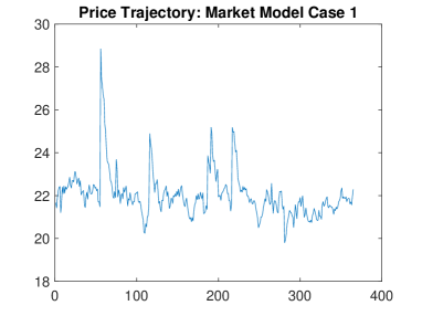
(a) Sample Trajectory.

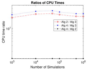
(b) Ratio of CPU times.

Table 2 shows the estimated prices, the RMSE’s (divided by the squared root of the number of simulations) and the overall CPU times in seconds using the different methodologies for the simulation of the process $Y(t)$. As expected, in terms of convergence, all the approaches are equally performing while instead, the CPU times are radically different. Algorithm 2 and Algorithm 4 have similar computational effort therefore their CPU times are comparable as observed in Figure 1(b). On the other hand, our methodology provides a remarkable computational advantage: what requires minutes for the Algorithms 2 and 4 only requires seconds for the Algorithm 3. For example with $N=5\times 10^{5}$ simulations, with our computer, the pricing of the Asian option above, is accomplished in almost two minutes whereas, it takes almost one hour with the other alternatives. Figure 1(b) clearly shows that, in the worst case, our simulation procedure is at least thirty times faster than any other alternative being then suitable for real-time applications.

4.2 Numerical Experiments: Gas Storages

Denote by $C(t)$ the volume of a (virtual) gas storage at time $t$ with $C_{min}\leq C(t)\leq C_{max}$. The holder of such an energy asset is faced with a timing problem that consists in deciding when to inject, to withdraw or to do-nothing.

Denoting $J(t,x,c)$ the value of a gas storage at time $t$ given $S(t)=x$, $C(t)=c$, one can write:

$$J(t,x,c)=\sup_{u\in\mathcal{U}}\mathbb{E}\left[\int_{t}^{T}\phi_{u}\left(S(s)\right)ds+q\left(S(T),C(T)\right)\,\right|S(t)=x,C(t)=c\bigg{]},$$ (27)

where $\mathcal{U}$ denotes the set of the admissible strategies, $u(t)\in\{-1,0,1\}$ is the regime at time $t$ such that

$$\left\{\begin{array}[]{lcll}\phi_{-1}(S(t))&=&-S(t)-K_{in}a_{in},&\text{injection}\\ \phi_{0}(S(t))&=&-K_{N},&\text{do nothing}\\ \phi_{1}(S(t))&=&S(t)-K_{out}a_{w}&\text{withdrawal}\end{array}\right.,$$ (28)

$a_{in}$ and $a_{w}$ are the injection and withdrawal rates, $K_{in}$, $K_{out}$ and $K_{N}$, respectively, represent the costs of injection, do-nothing and withdrawal, and $q$ takes into account the possibility of final penalties. Based on the Bellman recurrence equation (see Bertsekas [6]), one can perform the following backward recursion for $i=1,\dots,d$:

$$J(t_{i},x,c)=\sup_{k\in\{-1,0,1\}}\left\{\phi_{k}S(t_{i})+\mathbb{E}\left[J\left(t_{i+1},S(t_{i+1}),\tilde{c}_{k}\right)|S(t_{i})=x,C(t_{i})=c\right]\right\},i=1,\dots,d,$$ (29)

where

$$\left\{\begin{array}[]{lll}\tilde{c}_{-1}&=&\min(c+a_{in},C_{max})\\ \tilde{c}_{0}&=&c\\ \tilde{c}_{1}&=&\min(c-a_{w},C_{min}).\\ \end{array}\right.$$ (30)

A standard approach to price gas storages is a modified version of the Least-Squares Monte Carlo (LSMC), introduced in Longstaff-Schwartz [22], detailed in Boogert and de Jong [7]. With this approach, the backward recursion is obtained by defining a finite volume grid of G steps for the admissible capacities $c$ of the plant and then apply the LSMC methodology to the continuation value per volume step. In alternative, one may solve the recursion by adapting the method proposed by Ben-Ameur et al. [3] or might use the quantization method as explained in Bardou et al. [1]. Although the LSMC might not be the fastest solution, risk management units of energy companies are often interested in quantiles of the price distribution that can be obtained as a side product using the LSMC method.

We focus then on the LSMC methodology and perform a few numerical experiments selecting the three-factors spot model with the jump component covered by the second case in Section 2 because we want to capture asymmetric jumps (we set $H(0)=0)$: in this case, because of (3) and (20) for $\beta_{1},\beta_{2}>1$ it results

$$h(t)=-\frac{\sigma_{D}^{2}}{4k_{D}}\left(1-e^{-2k_{D}t}\right)-\frac{\lambda_{1}}{k_{1}}\log\left(\frac{\beta_{1}-e^{-k_{1}t}}{\beta_{1}-1}\right)-\frac{\lambda_{2}}{k_{2}}\log\left(\frac{\beta_{2}-e^{-k_{2}t}}{\beta_{2}-1}\right).$$

Table 3: Parameters for Spot (day-ahead) dynamics (Case 2)

$S_{0}$	$k_{D}$	$\sigma_{D}$	$k_{1}$	$k_{2}$	$\lambda_{1}$	$\lambda_{2}$	$\beta_{1}$	$\beta_{2}$
$22$	$67$	$0.25$	$50$	$40$	$20$	$20$	$10$	$20$

This model can also be extended to cover correlated Poisson processes. For instance, in Cufaro Petroni and Sabino [11] and [12] we once more used the concept of sd to produce correlated Poisson processes with a time-delay mechanism among jumps, and we discussed an application to the pricing of spread options. Nevertheless, in this study we consider independent Poisson processes only.

Going back to the initial problem, we assume that the units of $C(0),C(T)$ and $C_{max}$ are in MWh, those of the injection and withdrawal rates are in MWh/day, whereas $S_{0}$ can be taken in €/MWh; in addition we suppose a flat forward curve. The remaining model parameters are shown in Table 3 and can be considered realistic.

We consider finally a one-year fast-churn storage with the parameters shown in Table 4 such that $20$ days are required to fill or empty the storage as shown in Figure 2(a).

$C(0)$	$C(T)$	$a_{in}$	$a_{w}$	$C_{max}$
0	0	$1$	$1$	$20$

Table 4: Fast Storage Specification.

	Algorithm 3			Algorithm 2			Algorithm 4
$N$	Price	LSMC	PATH	Price	LSMC	PATH	Price	LSMC	PATH
$10^{3}$	$282.7$	$8.5$	$0.3$	$282.9$	$15.3$	$6.03$	$281.3$	$16.7$	$7.4$
$10^{4}$	$285.6$	$136.3$	$1.8$	$286.7$	$186.6$	$57.09$	$285.8$	$198.7$	$69.2$
$2\times 10^{4}$	$287.7$	$237.2$	$3.3$	$287.2$	$357.1$	$113.85$	$287.0$	$381.3$	$138.1$
$5\times 10^{4}$	$287.4$	$674.7$	$8.3$	$286.8$	$1002.1$	$290.34$	$286.8$	$1063.7$	$351.9$
$10^{5}$	$287.5$	$1197.0$	$17.9$	$287.0$	$1818.3$	$582.05$	$286.9$	$1936.5$	$700.3$

Table 5: Storages: Overall CPU times in seconds (LSMC), CPU times relative to the path generation (PATH) and comparison among the prices obtained with the different algorithms

Figure 2: Gas Storages.

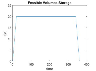
(a) Feasible Volumes of the fast churn storage

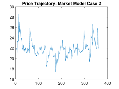
(b) Sample Trajectory

Figure 3: Gas Storage Results.

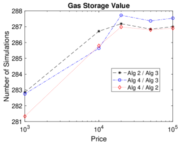
(a) Values Gas Storage.

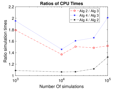
(b) Ratio of CPU Times.

In line with that observed for the pricing of Asian options, Table 5 and Figure 3(a) show that the three types of implementation apparently return comparable gas storage values. On the other hand, the ratio of overall CPU times in Figure 3(b) is not as extreme compared to the Asian option case. Algorithm 3 is “only” $40\%$ faster, in the worst case, compared to the other two solutions. The reason of this apparent different conclusion compared to the previous section is that the main component to the overall computational cost derives from the stochastic optimization. To this end, Table 5 also displays the CPU times required for the path simulation only (denoted PATH) where one can observe the Algorithm 3 is once again tens of times faster. Using Algorithms 2 and 4 the path simulation time is a relevant portion of the overall time, whereas using our approach it is, as if the overall cost coincides with that required by the purely LSMC stochastic optimization. This fact provides a computational advantage when one needs to calculate the sensitivities of the storage because a high number of simulations is required.

We finally remark that Algorithm 1 relies on the sequential simulation of the price trajectory forward in time. In combination with LSMC methods, this is not the optimal approach because the entire set of trajectories and simulations are stored in memory with a risk of memory allocation issues. For instance, Pellegrino and Sabino [26] and Sabino [28] have shown that the backward simulation is preferable with LSMC. Unfortunately, although we know the law of the standard Gaussian-OU bridge, we do not know the law of the $\Gamma$-OU bridge which will be one of the topics of our future studies.

4.3 Numerical Experiments: Swings

A swing option is a type of contract used by investors in energy markets that lets the option holder buy a predetermined quantity of energy at a predetermined price (strike), while retaining a certain degree of flexibility in both the amount purchased and the price paid. Such a contract can also be seen as a simplified gas storage where $a_{in}=0$, $K_{N}=0$ and $K_{w}$ is the strike of the contract. We consider a $120$-$120$ swing with the specifications of Table 7 and Figure 5(a): it can be seen as plugging $C(0)=120$, $C(T)=0$, $a_{in}=0$, $a_{w}=1$, $C_{max}=120$ into (27) with an injection cost equal to the strike.

In this last example, we now choose the third market model in Section 2 that consists in a two-factors model with one Gaussian OU diffusion and one symmetric $\mathrm{bi}\Gamma$-OU process - a compound Poisson with Laplace jumps - where once more we set $H(0)=0$. We also consider a step-wise daily approximation of the following time-dependent intensity

$$\lambda(t)=\frac{2\theta}{1+|sin\left(\pi\omega(t-\tau)\right)|}$$ (31)

so that for $m=1,\dots,M$ and $\beta>1$ we have

$$h(t_{m})=\frac{\sigma_{D}^{2}}{4k_{D}}\left(1-e^{-2k_{D}t_{m}}\right)-\frac{\lambda_{m}}{2k}\log\left(\frac{\beta^{2}-e^{-2kt_{m}}}{\beta^{2}-1}\right)$$

with the parameters of Table 6 once again with a flat forward curve. The value of $\theta$ is such that the average number of jumps per year is about $40$ as in the storage example.

Table 6: Parameters for Spot (day-ahead) dynamics (Case 3)

$S_{0}$	$k_{D}$	$\sigma_{D}$	$k_{N}$	$\theta$	$\omega$	$\tau$	$\beta$
$22$	$67$	$0.25$	$50$	$32$	$2$	$0.25$	$20$

$ACQmin$	$ACQmax$	$DCQmin$	$DCQmax$	$T(days)$
120	120	$1$	$1$	$360$

Table 7: Specification of 120-120 take-or-pay Swing

	Algorithm 6			Algorithm 5			Algorithm 7
$N$	Price	LSMC	PATH	Price	LSMC	PATH	Price	LSMC	PATH
$10^{3}$	$118.0$	$7.2$	$0.2$	$117.2$	$12.3$	$5.32$	$120.2$	$13.6$	$5.3$
$10^{4}$	$117.6$	$137.2$	$1.2$	$117.1$	$181.8$	$50.45$	$118.7$	$193.9$	$50.4$
$2\times 10^{4}$	$117.9$	$237.4$	$2.4$	$117.5$	$335.9$	$102.04$	$118.4$	$360.1$	$102.0$
$5\times 10^{4}$	$118.0$	$625.4$	$5.7$	$117.9$	$849.2$	$257.82$	$118.5$	$910.8$	$257.8$
$10^{5}$	$118.0$	$1147.2$	$11.7$	$117.6$	$1603.5$	$519.85$	$118.2$	$1721.7$	$519.8$

Table 8: Swings: Overall CPU times in seconds (LSMC), CPU times relative to the path generation (PATH) and comparison among the prices obtained with the different algorithms

Figure 4: Market Model.

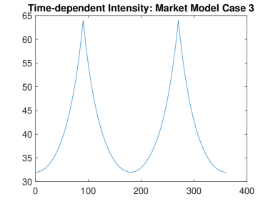
(a) Time-dependent Intensity

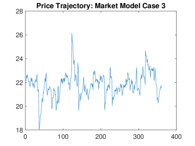
(b) Sample Trajectory.

Figure 5: Swings.

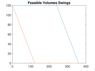
(a) Feasible Volumes of a $120$-$120$ Swing.

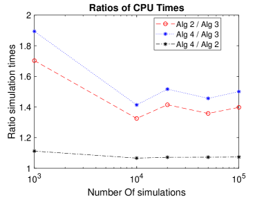
(b) Swing Values and Ratio of CPU times.

Due to the fact that jump component has now symmetric Laplace jumps, the process $Y(t)$ can be seen as a symmetric $\mathrm{bi}\Gamma$-OU process therefore, instead of executing Algorithms 2, 3 and 4 two times, we can rely on Algorithms 5, 6 and 7. The conclusions that we can derive from the numerical experiments are very much in line with what is observed in the case of gas storages. As expected, the MC based estimated values of the swing option obtained with the three types of implementation are similar.

As shown in Table 8 and Figure 5(b), once more the CPU times with Algorithm 6 are far lower resulting in a competitive advantage of about $40\%$ (in the worst case) on the overall computational cost (LSMC in Table 8). This factor becomes even higher if one focuses on the time required to simulate the price paths (PATH in Table 8). The contribution of the stochastic optimization step to the overall cost is again of about $75\%$ using Algorithm 5 or Algorithm 7, while instead, with Algorithm 6, the path generation step becomes almost negligible compared to the total CPU time. We can therefore conclude that Algorithm 6 is the preferable solution for the simulation of the jump component in the market model (4).

5 Conclusions and future inquiries

In this paper we have considered the problem of pricing complex energy derivatives with Monte Carlo simulations using mean-reverting jump-diffusion market models. The jump component that we have chosen is a compound Poisson process with exponentially or bilateral exponentially distributed jumps known in the literature as $\Gamma$-OU or $\mathrm{bi}\Gamma$-OU processes. Although, this is a simple and standard approach, the simulation of the price trajectories may soon become very computational expensive, especially for the pricing of complex derivative contracts. Indeed, the generation of the path of the jump process has a relevant impact on the overall computational cost.

Based on our results in Cufaro Petroni and Sabino [13], the main contribution of this paper is the design of exact and very fast simulation algorithms for the simulation of the spot prices that potentially could be used for real-time pricing.

We illustrated the applications of our findings in the context of the pricing of Asian options with standard Monte Carlo and gas storages and swings adopting the Least-Squares Monte Carlo method introduced in Boogert and de Jong[7]. The overall computational effort depends on the cost of simulating the price trajectories and the stochastic optimization (this last step is not influenced by the particular simulation algorithm).

We have conducted extensive simulation experiments and compared the performance of our proposal to the traditional approach of Cont and Tankov [9] and a recent methodology described by Qu et al. [27]. Our numerical experiments have shown that our solution outperforms any other alternative, because it cuts the simulation time down by a factor larger than forty in the case of Asian options and to a factor of forty percent for the gas storages and swings. In contrast to the other approaches, the numerical tests suggest that our simulation methodology is suitable for real-time pricing.

From a mathematical point of view, it would be interesting to study if – and under which conditions – our results could be generalized to other Ornstein-Uhlenbeck processes used in financial applications and in energy markets (see for instance Cummins et al.[14]).

In a primarily economic and financial perspective, the future studies could cover the extension to a multidimensional setting with correlated Poisson processes as those introduced for instance in Lindskog and McNeil [21] or in Cufaro Petroni and Sabino [11]. A last topic deserving further investigation is a possible enhancement of the computational speed relying on backward simulations generalizing the results of Pellegrino and Sabino [26] and Sabino [28] to the case of $\Gamma$-OU or $\mathrm{bi}\Gamma$-OU processes.

References

- [1] O. Bardou, S. Bouthemy, and G. Pagés. Optimal Quantization for the Pricing of Swing Options. Applied Mathematical Finance, 16(2):183–217, 2009.
- [2] O.E. Barndorff-Nielsen and N. Shephard. Non-Gaussian Ornstein-Uhlenbeck-based Models and Some of Their Uses in Financial Economics. Journal of the Royal Statistical Society: Series B, 63(2):167–241, 2001.
- [3] H. Ben-Ameur, M. Breton, L. Karoui, and P. L’Ecuyer. A Dynamic Programming Approach for Pricing Options Embedded in Bonds. Journal of Economic Dynamics and Control, 31(7):2212–2233, July 2007.
- [4] F.E. Benth and A. Pircalabu. A non-gaussian Ornstein-Uhlenbeck Model for Pricing Wind Power Futures. Applied Mathematical Finance, 25(1), 2018.
- [5] F.E. Benth and J. Kallsen T. Meyer-Brandis. A non-Gaussian Ornstein-Uhlenbeck Process for Electricity Spot Price Modeling and Derivatives Pricing. Applied Mathematical Finance, 14(2):153–169, 2007.
- [6] D. P. Bertsekas. Dynamic Programming and Optimal Control, Volume I. Athena Scientific, Belmont, Mass., third edition, 2005.
- [7] A. Boogert and C. de Jong. Gas Storage Valuation Using a Monte Carlo Method. Journal of Derivatives, 15:81–91, 2008.
- [8] A. Cartea and M. Figueroa. Pricing in Electricity Markets: a Mean Reverting Jump Diffusion Model with Seasonality. Applied Mathematical Finance, No. 4, December 2005, 12(4):313–335, 2005.
- [9] R. Cont and P. Tankov. Financial Modelling with Jump Processes. Chapman and Hall, 2004.
- [10] N. Cufaro Petroni. Self-decomposability and Self-similarity: a Concise Primer. Physica A, Statistical Mechanics and its Applications, 387(7-9):1875–1894, 2008.
- [11] N. Cufaro Petroni and P. Sabino. Coupling Poisson Processes by Self-decomposability. Mediterranean Journal of Mathematics, 14(2):69, 2017.
- [12] N. Cufaro Petroni and P. Sabino. Pricing exchange options with correlated jump diffusion processes. Quantitative Finance, pages 1–13, 2018.
- [13] N. Cufaro Petroni and P. Sabino. Gamma Related Ornstein–Uhlenbeck Processes and their Simulation. available at: https://arxiv.org/abs/2003.08810, 2020.
- [14] M. Cummins, G. Kiely, and B. Murphy. Gas Storage Valuation under Lévy Processes using Fast Fourier Transform. Journal of Energy Markets, 4:43–86, 2017.
- [15] S. Deng. Stochastic Models of Energy Commodity Prices and Their Applications: Mean-reversion with Jumps and Spikes. Citeseer, 2000.
- [16] B. Hambly, S. Howison, and T. Kluge. Information-Based Models for Finance and Insurance. Quantitative Finance, 9(8):937–949, 2009.
- [17] M. Kjaer. Pricing of Swing Options in a Mean Reverting Model with Jumps. Applied Mathematical Finance, 15(5-6):479–502, 2008.
- [18] T. Kluge. Pricing Swing Options and other Electricity Derivatives. Technical report, University of Oxford, 2006. PhD Thesis, Available at http://perso-math.univ-mlv.fr/users/bally.vlad/publications.html.
- [19] S. G. Kou. A Jump-Diffusion Model for Option Pricing. Manage. Sci., 48(8):1086–1101, August 2002.
- [20] U. Küchler and S. Tappe. Bilateral Gamma Distributions and Processes in Financial Mathematics. Stochastic Processes and their Applications, 118(2):261–283, 2008.
- [21] F. Lindskog and J. McNeil. Common poisson shock models: applications to insurance and credit risk modelling. ASTIN Bulletin, 33(2):209–238, 2003.
- [22] F. A. Longstaff and E.S. Schwartz. Valuing American Options by Simulation: a Simple Least-Squares Approach. Review of Financial Studies, 14(1):113–147, 2001.
- [23] J.J. Lucia and E.S. Schwartz. Electricity Prices and Power Derivatives: Evidence from the Nordic Power Exchange. Review of Derivatives Research, 5(1):5–50, Jan 2002.
- [24] E. McKenzie. Innovation Distridution for Gamma and Negative Binomial Autoregressions. Scandinavian Journal of Statistics: Theory and Applications, 14(1):79–85, 1987.
- [25] T. Meyer-Brandis and P. Tankov. Multi-factor Jump-diffusion Models of Electricity Prices. International Journal of Theoretical and Applied Finance, 11(5):503–528, 2008.
- [26] T. Pellegrino and P. Sabino. Enhancing Least Squares Monte Carlo with Diffusion Bridges: an Application to Energy Facilities. Quantitative Finance, 15(5):761–772, 2015.
- [27] Y. Qu, A. Dassios, and H. Zhao. Exact Simulation of Gamma-driven Ornstein–Uhlenbeck Processes with Finite and Infinite Activity Jumps. Journal of the Operational Research Society, 0(0):1–14, 2019.
- [28] P. Sabino. Forward or Backward Simulations? A Comparative Study. Quantitative Finance, 2020. In press.
- [29] K. Sato. Lévy Processes and Infinitely Divisible Distributions. Cambridge U.P., Cambridge, 1999.
- [30] W. Schoutens. Lévy Processes in Finance: Pricing Financial Derivatives. John Wiley and Sons Inc, 2003.
- [31] P. Schwartz and J.E. Smith. Short-term Variations and Long-term Dynamics in Commodity Prices. Management Science, 46(7):893–911, 2000.