QCD in the heavy dense regime for general $N_{c}$ :
On the existence of quarkyonic matter

Abstract

Lattice QCD with heavy quarks reduces to a three-dimensional effective theory of Polyakov loops, which is amenable to series expansion methods. We analyse the effective theory in the cold and dense regime for a general number of colours, $N_{c}$. In particular, we investigate the transition from a hadron gas to baryon condensation. For any finite lattice spacing, we find the transition to become stronger, i.e. ultimately first-order, as $N_{c}$ is made large. Moreover, in the baryon condensed regime, we find the pressure to scale as $p\sim N_{c}$ through three orders in the hopping expansion. Such a phase differs from a hadron gas with $p\sim N_{c}^{0}$, or a quark gluon plasma, $p\sim N_{c}^{2}$, and was termed quarkyonic in the literature, since it shows both baryon-like and quark-like aspects. A lattice filling with baryon number shows a rapid and smooth transition from condensing baryons to a crystal of saturated quark matter, due to the Pauli principle, and is consistent with this picture. For continuum physics, the continuum limit needs to be taken before the large $N_{c}$ limit, which is not yet possible in practice. However, in the controlled range of lattice spacings and $N_{c}$-values, our results are stable when the limits are approached in this order. We discuss possible implications for physical QCD.

1 Introduction

The QCD phase diagram is important for many aspects of current nuclear, heavy ion and astro-particle physics, yet it remains largely unknown. This is because lattice QCD at finite baryon chemical potential has a severe sign problem, which prohibits straightforward Monte Carlo simulations. Various workarounds to extend the Monte Carlo method introduce additional approximations and are limited to the high temperature and/or low density region, with baryon chemical potential $\mu_{B}/T\raise 1.29167pt\hbox{$<$\kern-7.5pt\raise-4.73611pt\hbox{$\sim$}}3$ review . No sign of criticality is found in this region, where the transition from a hadronic gas to a quark gluon plasma proceeds by an analytic crossover aoki ; pastor ; bazavov ; vov . The same conclusion is reached by analytic non-perturbative approaches like Dyson-Schwinger equations cf or the functional renormalisation group jp . Despite continuing efforts, a genuine solution to the sign problem, and hence fully non-perturbative access to the cold and dense region of QCD, are missing to date.

This situation has motivated the study of QCD also in unphysical, but controllable parameter regions, where the sign problem can be overcome by either algorithmic or analytic methods. In this work our goal is to bridge two such approaches. We employ an effective lattice theory derived from the standard Wilson action by combined strong coupling and hopping (inverse quark mass) expansions. The effective theory is valid on reasonably fine lattices, as long as the quarks are sufficiently heavy to be described by the next-to-next-to-leading order in the hopping expansion. In this parameter range the theory correctly reproduces the critical heavy quark mass at zero density, where the first-order deconfinement transition changes to a smooth crossover fromm , and furthermore allows for an extension to finite baryon chemical potential, including the cold and dense regime around the onset transition to baryon matter.

Here we consider the effective theory for general colour gauge group $SU(N_{c})$, in order to establish contact with another effective approach in the continuum, namely QCD at large $N_{c}$. In particular, we analyse thermodynamic functions around the onset transition to baryon matter in the cold and dense regime, for varying and large $N_{c}$. This allows us to address, by direct calculation, various conjectures made in quarky regarding the phase diagram and the effective degrees of freedom at large $N_{c}$. There, the authors argue for the existence of quarkyonic matter, which is characterised by its pressure scaling as $p\sim N_{c}$ and has both baryon-like and quark-like aspects. Phenomenological consequences of this form of matter in physical QCD have been assessed in anton ; spirals ; pheno ; reddy . A general, qualitative discussion about the possibilities for the phase diagram in $(T,\mu,N_{c})$-space as well as references to earlier work can be found in mish .

We begin with a brief review of the effective lattice theory in section 2. This material is not new and can be skipped by readers familiar with it, but is needed as reference point when interpreting the following results. In section 3, a summary of the conjectured phase diagram at large $N_{c}$ is followed by our proper calculations for general $N_{c}$ and the analysis of the results for large $N_{c}$. Finally, section 4 concludes what is expected for physical QCD.

2 QCD with heavy quarks

2.1 The effective lattice theory

Consider the partition function of lattice QCD with the standard Wilson action at finite temperature, $T=1/(aN_{\tau})$, realised by compact euclidean time with $N_{\tau}$ slices and (anti-) periodic boundary conditions for (fermions) bosons. An entirely equivalent formulation in terms of temporal lattice links only is obtained after performing the Gauss integral over the quark fields and integrating the gauge links in spatial directions,

$$Z=\int DU_{0}DU_{i}\;\det Q\;e^{-S_{g}[U]}\equiv\int DU_{0}\;e^{-S_{\mathrm{eff}}[U_{0}]}=\int DW\,\;e^{-S_{\mathrm{eff}}[W]}\;.$$ (1)

With the spatial links gone, the effective action depends on the temporal links only via Wilson lines closing through the periodic boundary,

$$W({\bf x})=\prod_{\tau=1}^{N_{\tau}}U_{0}({\bf x},\tau)\;.$$ (2)

For $SU(2)$ and $SU(3)$ the effective action can always be expressed in terms of Polyakov loops, $L({\bf x})={\rm Tr}W({\bf x})$, whereas for larger $N_{c}$ in general traces of higher powers of $W$ appear as well.

This effective action is unique and exact. However, the integration over spatial links causes long-range interactions of Polyakov loops at all distances and to all powers so that in practice truncations are necessary. For non-perturbative ways to define and determine truncated theories, see wozar ; green1 ; green2 ; bergner . Here, we use an effective theory based on expanding the path integral in a combined character and hopping parameter series. Both expansions result in convergent series within a finite radius of convergence (for an introduction, see mm ). Truncating these at some finite order, the integration over the spatial gauge links can be performed analytically to provide a closed expression for the effective theory. Going via an effective action results in a resummation to all powers with better convergence properties compared to a direct series expansion of thermodynamic observables as in lange1 ; lange2 ; p_nc . Since the Wilson line $W({\bf x})$ contains the length $N_{\tau}$ of the temporal lattice extent implicitly, the effective theory is three-dimensional. Note that, in the case of 4d Yang-Mills theory, this representation by a 3d centre-symmetric effective theory is the basis for the Svetitsky-Yaffe conjecture sy ; polon concerning the universality of $SU(N_{c})$ deconfinement transitions. Including the quark determinant via the hopping expansion introduces centre symmetry breaking terms and additional effective couplings.

Let us briefly summarise the expansions used in order to perform the spatial link integrations. The gauge part of the action is a class function with respect to the product of the links of one plaquette:

$$S_{g}[U]=\sum_{p}S_{g,p}(U_{p})=\sum_{p}S_{g,p}(V^{-1}U_{p}V),$$ (3)

where $V\in SU(N_{c})$. Therefore it can be expanded in the characters $\chi_{r}$ of the irreducible representations $r$ of $SU(N_{c})$ at every plaquette,

$$e^{-S_{g,p}(U_{p})}=c_{0}\Big{(}1+\sum_{r\neq 0}d_{r}a_{r}(\beta)\chi_{r}(U_{p})\Big{)}\;.$$ (4)

In this formula, $d_{r}$ denotes the dimension of the representation and $a_{r}(\beta)$ is the character expansion coefficient divided by the expansion coefficient of the trivial representation. The expansion coefficients can be computed exploiting the orthogonality of the characters:

$$a_{r}(\beta) =\frac{c_{r}(\beta)}{c_{0}(\beta)},$$ (5)

$$c_{r}(\beta) =\int\limits_{SU(N_{c})}dU\chi_{r}(U)^{\ast}\exp(-S_{g,p}(U)).$$ (6)

We drop the overall factor of $c_{0}$ in equation (4), as it cancels in expectation values. For the integration of the spatial links following this expansion, one can use the formulas

$$\int\limits_{SU(N_{c})}dU\;\chi_{r}(UV)\chi_{s}(WU^{-1}) =\delta_{rs}\frac{1}{d_{r}}\chi_{r}(VW)\;,$$ (7)

$$\int\limits_{SU(N_{c})}dU\;\chi_{r}(UVU^{-1}W) =\frac{1}{d_{r}}\chi_{r}(V)\chi_{r}(W)\;,$$ (8)

for those cases where not more than two non-trivial representations share a common link. In earlier publications efft1 this was used to derive the effective gauge action for $SU(3)$ to rather high orders in the coefficient of the fundamental character $u(\beta)\equiv a_{f}(\beta)/d_{f}=a_{f}(\beta)/N_{c}$. The coefficients of the higher dimensional representations can be expressed in terms of the fundamental one, see also section 3.1, and therefore the expansion can be organised according to powers of the fundamental character. The dependence of $u$ on the lattice gauge coupling $\beta=2N_{c}/g^{2}$ can be specified either as a power series or numerically,

$$u(\beta)=\frac{\beta}{18}+\frac{\beta^{2}}{216}+\ldots<1.$$ (9)

It is known to arbitrary precision, and $u$ is always smaller than one for finite $\beta$-values.

For the hopping expansion it is useful to split the quark matrix in temporal and spatial hops between nearest neighbours,

$$Q =1-T-S,$$ (10)

$$\det(Q) =\det(1-T)\det(1-(1-T)^{-1}S)$$ (11)

$$=\det(Q_{\mathrm{stat}})\det({Q_{\mathrm{kin}}})\;.$$ (12)

This is because the static determinant containing all temporal hops (and only those) can be computed exactly hetrick ; bind . We then do the hopping expansion of the kinetic quark determinant using

$$\det{Q_{\mathrm{kin}}}=\exp({\rm Tr}(\ln(Q_{\mathrm{kin}})))\;.$$ (13)

This leads to an expansion in powers of $S$, which is proportional to the hopping parameter,

$$\kappa=\frac{1}{2am_{q}+8}\;.$$ (14)

The expansion terms are then ordered according to their number of spatial hops while the temporal ones are resummed to all orders. Since the hopping expansion is in inverse quark mass, the effective theory to low orders is valid for heavy quarks only. For a derivation of the effective theory to order $\mathcal{O}(\kappa^{4})$ in spatial hops, see bind . In this case the relevant integrals for the fermionic contributions are

$$\int\limits_{SU(N_{c})}dU\;U_{ij}U_{kl}^{\dagger} =\frac{1}{N_{c}}\delta_{il}\delta_{jk},$$ (15)

$$\begin{split}\int\limits_{SU(N_{c})}dU\;U_{i_{1}j_{1}}U_{i_{2}j_{2}}U^{\dagger}_{k_{1}l_{1}}U^{\dagger}_{k_{2}l_{2}}&=\frac{1}{N_{c}^{2}-1}\Big{[}\delta_{i_{1}l_{1}}\delta_{i_{2}l_{2}}\delta_{j_{1}k_{1}}\delta_{j_{2}k_{2}}+\delta_{i_{1}l_{2}}\delta_{i_{2}l_{1}}\delta_{j_{1}k_{2}}\delta_{j_{2}k_{1}}\Big{]}\\ &\quad-\frac{1}{N_{c}(N_{c}^{2}-1)}\Big{[}\delta_{i_{1}l_{2}}\delta_{i_{2}l_{1}}\delta_{j_{1}k_{1}}\delta_{j_{2}k_{2}}+\delta_{i_{1}l_{1}}\delta_{i_{2}l_{2}}\delta_{j_{1}k_{2}}\delta_{j_{2}k_{1}}\Big{]}.\end{split}$$ (16)

Generically, the effective action obtained in this way has the following form:

$$-S_{\mathrm{eff}}=\sum_{i=1}^{\infty}\lambda_{i}(u,\kappa,N_{\tau})S_{i}^{s}-2N_{f}\sum_{i=1}^{\infty}\left[h_{i}(u,\kappa,\mu,N_{\tau})S_{i}^{a}+\bar{h}_{i}(u,\kappa,\mu,N_{\tau})S_{i}^{a,\dagger}\right]\;.$$ (17)

The $\lambda_{i}$ are defined as the effective couplings of the $Z(N_{c})$-symmetric terms $S_{i}^{s}$, whereas the $h_{i}$ multiply the asymmetric terms $S_{i}^{a}$. In particular, $h_{1},\bar{h}_{1}$ are the coefficients of $L,L^{*}$, respectively, and to leading order correspond to the fugacity of the quarks and anti-quarks,

$$h_{1} = (2\kappa)^{N_{\tau}}e^{a\mu N_{\tau}}(1+\ldots)=h_{1}^{\rm LO}(1+\ldots)=e^{\frac{\mu-m}{T}}(1+\ldots)\;,$$ (18)

$$\bar{h}_{1} = (2\kappa)^{N_{\tau}}e^{-a\mu}(1+\ldots)=\bar{h}_{1}^{\rm LO}(1+\ldots)=e^{-\frac{\mu+m}{T}}(1+\ldots)\;.$$ (19)

Here,

$$am=\ln(2\kappa)=\frac{am_{B}^{\mathrm{LO}}}{N_{c}}$$ (20)

is the constituent quark mass in lattice units of a baryon computed to leading order in the hopping expansion ks , while

$$h_{2}=\kappa^{2}N_{\tau}/N_{c}(1+\ldots)$$ (21)

is the effective coupling of a nearest neighbour $L_{\bf x}L_{\bf y}$ interaction.

The partition function for $SU(3)$, including just these simplest interactions, reads

$$Z = \int DW\prod_{<{\bf x},{\bf y}>}\left[1+\lambda_{1}(L_{{\bf x}}L_{{\bf y}}^{*}+L_{{\bf x}}^{*}L_{{\bf y}})\right]$$

$$\times\prod_{{\bf x}}[1+h_{1}L_{{\bf x}}+h_{1}^{2}L_{{\bf x}}^{*}+h_{1}^{3}]^{2N_{f}}[1+\bar{h}_{1}L^{*}_{{\bf x}}+\bar{h}_{1}^{2}L_{{\bf x}}+\bar{h}_{1}^{3}]^{2N_{f}}$$

$$\times\prod_{<{\bf x},{\bf y}>}\left(1-h_{2}{\rm Tr}\frac{h_{1}W_{{\bf x}}}{1+h_{1}W_{{\bf x}}}{\rm Tr}\frac{h_{1}W_{{\bf y}}}{1+h_{1}W_{{\bf y}}}\right)\left(1-h_{2}{\rm Tr}\frac{\bar{h}_{1}W^{\dagger}_{{\bf x}}}{1+\bar{h_{1}}W^{\dagger}_{{\bf x}}}{\rm Tr}\frac{\bar{h}_{1}W^{\dagger}_{{\bf y}}}{1+\bar{h}_{1}W^{\dagger}_{{\bf y}}}\right)\times\ldots\;.$$

In this expression the first line represents the pure gauge sector, the second line is the static determinant and the third line the leading correction from spatial quark hops. This partition function has a weak sign problem and can be simulated with either reweighting or complex Langevin methods fromm ; bind . Since the effective couplings correspond to power series of the expansion parameters, they are themselves small in the range of validity. Hence, the effective theory can also be treated by linked-cluster expansion methods known from statistical physics, with results for thermodynamic observables in quantitative agreement with the numerical ones k8 . In this way, full control over the sign problem is achieved.

2.2 The deconfinement transition

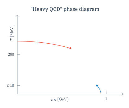
Figure 1: The phase diagram of QCD with very heavy quarks.

The phase diagram of QCD with heavy quarks is depicted schematically in Fig. 1. At zero density, the thermal transition is a first-order deconfinement transition. It is a remnant of the centre symmetry-breaking transition of the $SU(3)$ pure gauge theory, which gets weakened by explicitly centre-breaking finite quark masses $\sim 1/m_{q}$, until it ends in a second-order point for some critical mass $m_{q}^{c}$. In the effective theory, this phase transition appears as spontaneous breaking of the $Z(3)$-symmetry at some set of critical couplings $\lambda_{i,c}=\lambda_{i}(u_{c},\kappa_{c},N_{\tau}),h_{i,c}(u_{c},\kappa_{c},N_{\tau})$, which can be determined by numerical simulation. Inversion of the effective couplings then gives predictions for $\beta_{c}(N_{\tau}),\kappa_{c}(N_{\tau})$, which can be compared with the results from full QCD simulations.

For $SU(2)$ and $SU(3)$-Yang-Mills theory, the simplest effective theory with only a nearest neighbour coupling (first line in equation (2.1)) correctly reproduces the universality of the respective deconfinement transitions, and the predicted $\beta_{c}(N_{\tau})$ are within 10% of their true values for $N_{\tau}=2,\ldots,16$ efft1 . For QCD with heavy quarks, the simplest effective theory including the static determinant and $\kappa^{2}$-corrections, predicts $\kappa_{c}$ to better than 10% on $N_{\tau}=4$ fromm . Contrary to full QCD, the effective theory can be simulated at finite chemical potential to determine the location of the critical end point as a function of quark mass fromm . This qualitative behaviour of the deconfinement transition in the heavy quark region is also found by continuum studies using a Polyakov loop model lo and in the functional renormalisation group approach frg .

2.3 The onset transition to finite baryon number

Going out along the chemical potential axis at low temperature, the system crosses the onset transition beyond which the ground state consists of condensed baryon matter. In order to interpret our analysis for general $N_{c}$, let us first recall the situation for $N_{c}=3$ in some detail. The qualitative features are best understood in the strong coupling limit, $\beta=0$, with the static quark determinant only, where (2.1) is reduced to the second line. The partition function then factorises into one-site integrals which can be solved analytically. Since we are interested in low temperatures, where mesonic contributions are exponentially suppressed by their fugacity factors, we simplify the analysis by setting $\bar{h_{1}}=0$. For $N_{f}=1$ the partition function then reads silver ; bind

$$Z(\beta=0)\stackrel{{\scriptstyle T\rightarrow 0}}{{\longrightarrow}}z_{0}^{V}\quad\mbox{with}\quad z_{0}=1+4h_{1}^{3}+h_{1}^{6}\;,$$ (23)

corresponding to a free baryon gas with two species. With one quark flavour only, there are no nucleons and the first prefactor indicates a spin 3/2 quadruplet of $\Delta$-baryons whereas the second term is a spin 0 six-quark state or di-baryon. The quark number density is

$$n=\frac{T}{V}\frac{\partial}{\partial\mu}\ln Z=\frac{1}{a^{3}}\frac{4N_{c}h_{1}^{N_{c}}+2N_{c}h_{1}^{2N_{c}}}{1+4h_{1}^{N_{c}}+h_{1}^{2N_{c}}}\;,\quad\lim_{T\rightarrow 0}a^{3}n=\left\{\begin{array}[]{cc}0,&\mu<m\\ 2N_{c},&\mu>m\end{array}\right.\;,$$ (24)

and at zero temperature exhibits a discontinuity when the quark chemical potential equals the constituent mass $m$. This reflects the “silver blaze” property of QCD, i.e. the fact that the baryon number stays zero for small $\mu$ even though the partition function explicitly depends on it cohen . Once the baryon chemical potential $\mu_{B}=3\mu$ is large enough to make a baryon ($m_{B}=3m=m_{B}^{\mathrm{LO}}$ in the static strong coupling limit), a discontinuous phase transition to a saturated crystal takes place. Note that saturation density here is $2N_{c}$ quarks per flavour and lattice site and reflects the Pauli principle. This is clearly a discretisation effect that disappears in the continuum limit.

For two flavours the corresponding expression for the free baryon gas reads

$$z_{0} = (1+4h_{d}^{3}+h_{d}^{6})+(6h_{d}^{2}+4h_{d}^{5})h_{u}+(6h_{d}+10h_{d}^{4})h_{u}^{2}+(4+20h_{d}^{3}+4h_{d}^{6})h_{u}^{3}$$ (25)

$$+(10h_{d}^{2}+6h_{d}^{5})h_{u}^{4}+(4h_{d}+6h_{d}^{4})h_{u}^{5}+(1+4h_{d}^{3}+h_{d}^{6})h_{u}^{6}\;,$$

where we have now distinguished between the $h_{1}$ coupling for the $u$- and $d$-quarks. In this case we identify in addition the spin 1/2 nucleons as well as many other baryonic multi-quark states with their correct spin degeneracy. A similar result is obtained for mesons if we instead consider an isospin chemical potential in the low temperature limit bind . Again, the onset transition to finite baryon density is a step function from zero to saturation density, which now is $2N_{c}N_{f}$ quarks per site.

The step function behaviour gets immediately smeared out to a smooth crossover, as soon as a finite temperature, $N_{\tau}<\infty$, is switched on. This implies that the first-order line of the nuclear liquid gas transition is exponentially short as a result of the large quark masses, as expected from nuclear physics Yukawa potentials with meson exchange. Indeed, the interaction energy per baryon, which sets the scale for the critical endpoint of the nuclear liquid gas transition, can be extracted from the dimensionless combination of energy density and baryon number of the system,

$$\epsilon(\mu,T)=\frac{e(\mu,T)-n_{B}(\mu,T)m_{B}}{n_{B}(\mu,T)m_{B}}\;,$$ (26)

in the limit of zero temperature. In the strong-coupling limit one finds

$$\epsilon=-\frac{4}{3}\frac{1}{a^{3}n_{B}}\left(\frac{6h_{1}^{3}+3h_{1}^{6}}{z_{0}}\right)^{2}\,\kappa^{2}+\ldots\;.$$ (27)

Thus the length of the liquid gas transition in Fig. 1 is a function of quark mass and decreases to zero towards the static limit. Including $\kappa^{4}$-corrections, a first-order transition ending at some finite temperature is explicitly seen bind .

Including the gauge coupling, and with sufficiently many corrections at hand, also the lattice spacing can be varied and the approach to the continuum can be studied. In k8 it was shown that through orders $u^{5}\kappa^{8}$ for a sufficiently heavy quark mass, continuum-like behaviour is obtained immediately after the onset transition, with the qualitative features discussed here.

3 QCD for large $N_{c}$

Since in the framework of the effective theory we can work fully analytically, it is straightforward to investigate what happens when the number of colours $N_{c}$ is varied and made large. In particular, we aim to explore some large $N_{c}$ considerations leading to the prediction of quarkyonic matter quarky .

There is a lot of interesting literature on QCD at large $N_{c}$, which we are unable to represent properly. In particular, baryon matter in the combined heavy quark and large $N_{c}$ limits has been considered by a mean field analysis in the continuum cohen2 ; cohen3 . Here, our approach is quite different in working on the lattice with large but finite quark masses, for general $N_{c}$ and beyond mean field.

The essential qualitative features of QCD at lage $N_{c}$ were established in the early works hooft ; witten . The ’t Hooft limit is defined by

$$N_{c}\rightarrow\infty\quad\mbox{with}\quad\lambda_{H}\equiv g^{2}N_{c}={\rm const.}$$ (28)

In this case the theory has the following properties:

• Quark loops in Feynman diagrams are suppressed by $N_{c}^{-1}$

• Non-planar Feynman diagrams are suppressed by $N_{c}^{-2}$

• Mesons are free; the leading corrections are cubic interactions $\sim N_{c}^{-1/2}$ and quartic interactions $\sim N_{c}^{-1}$

• Meson masses are $\sim\Lambda_{QCD}$

• Baryons consist of $N_{c}$ quarks, baryon masses are $\sim N_{c}\Lambda_{QCD}$

• Baryon interactions are $\sim N_{c}$

The authors of quarky used these and various other ingredients to draw qualitative conclusions for the QCD phase diagram. Fig. 2 shows their conjectured phase diagram in the large $N_{c}$ limit. From finite temperature perturbation theory it follows that, in the plasma phase, $p\sim N_{c}^{2}$. With quark loops suppressed, the phase boundary of the deconfinement transition is pure gauge-like and unaffected by chemical potential. It thus forms a horizontal line, staying first-order everywhere. On the other hand, in the hadronic, low density phase, thermodynamics is quantitatively well described by a weakly interacting hadron resonance gas wb ; hotQCD . Statistical mechanics then implies that the baryonic contribution to the pressure is exponentially suppressed with baryon mass, so $p\sim N_{c}^{0}$ there. In quarky a similar combination of perturbative (valid for large $\mu$) and statistical mechanics arguments for baryons suggests that, for low temperatures and $\mu_{B}>m_{B}$, the pressure scales as $p\sim N_{c}$. The authors termed this phase “quarkyonic”, since it shows aspects of both quark matter and baryon matter. In particular it is argued that, for zero temperature, excitations relative to the Fermi sea should be baryon-like for $(p-p_{F})\raise 1.29167pt\hbox{$<$\kern-7.5pt\raise-4.73611pt\hbox{$\sim$}}\Lambda_{QCD}$ and quark-like for $(p-p_{F})\gg\Lambda_{QCD}$, implying a shell structure in momentum space as in Fig. 2 (right). Since the Fermi momentum is $p_{F}\raise 1.29167pt\hbox{$<$\kern-7.5pt\raise-4.73611pt\hbox{$\sim$}}\Lambda_{QCD}$ at the onset transition and then grows with quark chemical potential, this picture suggests the possibility to smoothly interpolate between baryon matter (right after the onset) and quark matter (at very large densities). We will now address these issues by direct calculations using the effective lattice theory.

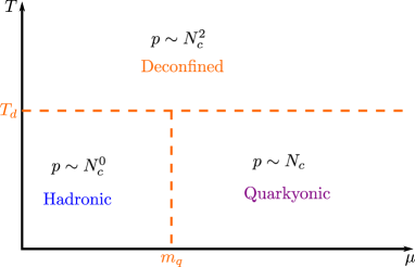
Figure 2: Left: Phase diagram in the limit of large $N_{c}$, as conjectured in quarky . Right: Quarkyonic matter in momentum space, with quark matter (Q) surrounded by a shell of baryons (B).

3.1 The effective lattice theory for general $N_{c}$

Note that $N_{c}=2$ has already been analysed in detail scior , with interesting physics results for two-colour QCD. Our aim here is to go in the other direction and to increase $N_{c}$. For the gluonic part, the derivation of the effective theory for general and large $N_{c}$ has already been discussed in myers . Note that the integration rules (7) and (8) are true for arbitrary $N_{c}$. Therefore, in cases where only these formulas are relevant, one simply has to replace $d_{r}$ and $a_{r}$ by their appropriate generalisations to $N_{c}$. Specifically, the character expansion coefficients $a_{r}$ can be obtained via Drouffe:1983fv

$$a_{r}(\beta/2N_{c})=\frac{1}{d_{r}}\sum_{n=-\infty}^{\infty}\det_{1\leq i,j\leq\infty}\left(I_{\alpha_{j}+i-j+n}(\beta/2N_{c})\right)\bigg{/}\sum_{n=-\infty}^{\infty}\det_{1\leq i,j\leq\infty}\left(I_{i-j+n}(\beta/2N_{c})\right).$$ (29)

In this formula, the $\alpha_{i}$ are a set of $N_{c}$ positive descending integers with $\alpha_{N_{c}}=0$ which label the representation and correspond to Young tableaux. Following Drouffe:1983fv one may re-express all coefficients of higher representations in terms of the fundamental representation using double Young tableaux. The characters corresponding to a double young tableau can be determined in terms of the traces of powers of $U$ and $U^{\dagger}$ Green:1980bg .

In myers the fermionic contributions were also discussed using the hopping expansion. However, only a subset of spatial hoppings to $\mathcal{O}(\kappa^{4})$ was considered, and temporal hoppings were included up to $\mathcal{O}(\kappa^{2N_{\tau}})$. As we mentioned in section 2, we work in a scheme where temporal hoppings are resummed to all orders. Nevertheless, equations (15) and (16) are valid for general $N_{c}$ so the fermionic contributions obtained in this way are legitimate also for general $N_{c}$.
Spatial baryon hoppings contribute at $\mathcal{O}(\kappa^{N_{c}})$ and therefore they are suppressed for large $N_{c}$. To evaluate the contributions of meson hoppings, integrals of the type

$$\int dU\;U_{i_{1}j_{1}}\cdots U_{i_{a}j_{a}}U_{k_{1}l_{1}}^{\dagger}\cdots U_{k_{a}l_{a}}^{\dagger}$$ (30)

are needed. Since these integrals give the same result for $U\in U(N_{c})$ and $U\in SU(N_{c})$ one can, for the fermionic contributions in the vacuum and at finite temperature, work with $U(N_{c})$ instead of $SU(N_{c})$ at large $N_{c}$. Likewise, when analysing the pure gauge theory for large $N_{c}$, the same simplification applies gw . However, at finite chemical potential temporal quark hoppings in the positive direction are boosted by a factor of $e^{a\mu}$ and therefore integrals of the type

$$\int dU\;U_{i_{1}j_{1}}\cdots U_{i_{a}j_{a}}U_{k_{1}l_{1}}^{\dagger}\cdots U_{k_{b}l_{b}}^{\dagger}$$ (31)

with

$$b-a=0\text{ mod }N_{c}$$ (32)

are relevant. These integrals vanish for $U(N_{c})$ when $b\neq a$, but not for $SU(N_{c})$, where they contain baryonic contributions. For the cold and dense regime, we therefore need to calculate integrals over $SU(N_{c})$.

3.2 Evaluation of the $SU(N_{c})$ effective theory in the strong coupling limit

We begin our analysis in the strong coupling limit, $u(\beta=0)=0$ and thus $\lambda_{1}=0,h_{1}=h_{1}^{\rm LO}$, and employ the effective theory to order $\mathcal{O}(\kappa^{4})$ in spatial hoppings. We also neglect terms containing $\bar{h}_{1}$, since they are exponentially suppressed at low temperatures. The theory with these approximations already shows the most salient features of baryon dynamics, and we discuss modifications by the neglected couplings in later sections. Thus we get the free energy density

$$\begin{split}-f&=\ln(z_{0})-6N_{f}\frac{\kappa^{2}N_{\tau}}{N_{c}}\left(\frac{z_{(11)}}{z_{0}}\right)^{2}\\ &\phantom{{}={}}+3\frac{\kappa^{4}N_{\tau}}{2(N_{c}^{2}-1)}\frac{4N_{f}^{2}z_{(22)}^{2}-4N_{f}z_{(11)^{2}}z_{(22)}+4N_{f}^{2}z_{(11)^{2}}^{2}}{z_{0}^{2}}\\ &\phantom{{}={}}-3\frac{\kappa^{4}N_{\tau}}{2(N_{c}^{2}-1)N_{c}}\frac{8N_{f}^{2}z_{(11)^{2}}z_{(22)}-2N_{f}z_{(11)^{2}}^{2}-2N_{f}z_{(22)}^{2}}{z_{0}^{2}}\\ &\phantom{{}={}}-3\frac{\kappa^{4}N_{\tau}(N_{\tau}-1)}{2N_{c}^{2}}\frac{4N_{f}^{2}z_{(11)^{2}}^{2}+4N_{f}^{2}z_{(21)}^{2}+2N_{f}z_{(21)}z_{(11)}+2N_{f}z_{(11)^{2}}z_{(21)}}{z_{0}^{2}}\\ &\phantom{{}={}}+30\frac{\kappa^{4}N_{\tau}}{N_{c}^{2}}\frac{N_{f}z_{(11)}^{2}\left(2N_{\tau}N_{f}z_{(11)^{2}}+(N_{\tau}-1)z_{(21)}+z_{(22)}+2z_{(11)}-4N_{c}\right)}{z_{0}^{3}}\\ &\phantom{{}={}}+12N_{f}\frac{\kappa^{4}N_{\tau}}{N_{c}^{2}}\left(\frac{z_{(11)}}{z_{0}}\right)^{3}-66N_{f}^{2}\frac{\kappa^{4}N_{\tau}^{2}}{N_{c}^{2}}\left(\frac{z_{(11)}^{4}}{z_{0}^{4}}\right),\end{split}$$ (33)

where we have introduced the notation

$$z_{0} =\int\limits_{SU(N_{c})}dW\det(1+h_{1}W)^{2N_{f}}\;,$$ (34)

$$z_{(a_{1}b_{1})\ldots(a_{k}b_{k})} =\int\limits_{SU(N_{c})}dW\det(1+h_{1}W)^{2N_{f}}\prod_{i=1}^{k}\frac{(h_{1}W)^{b_{i}}}{(1+h_{1}W)^{a_{i}}}\;.$$ (35)

The required integrals are related in the following way,

$$z_{(11)} =\frac{h_{1}}{2N_{f}}\frac{\partial}{\partial h_{1}}z_{0},$$ (36)

$$z_{(22)} =z_{(11)}-z_{(21)},$$ (37)

$$z_{(11)^{2}} =\frac{h_{1}}{2N_{f}}\frac{\partial}{\partial h_{1}}z_{(11)}-\frac{1}{2N_{f}}z_{(21)}\;.$$ (38)

Therefore, we only need to integrate $z_{0}$, which corresponds to the integration over the static determinant, and $z_{(21)}$. Note that all integrands are class functions of $SU(N_{c})$ group elements, $f(W)=f(VWV^{-1})$, which are invariant under a change of basis. These functions only depend on the eigenvalues $z_{i}$ of a group element. Furthermore, for our purposes it is sufficient to specialise to functions which factorise in the following way

$$f(W)=\tilde{f}(z_{1},\ldots,z_{N_{c}})=\sum_{\mu=1}^{N_{c}}\tilde{f}_{1,\mu}(z_{1})\cdot\ldots\cdot\tilde{f}_{N_{c},\mu}(z_{N_{c}})\;.$$ (39)

For such functions, the integration over the group can be expressed as Nishida:2003fb

$$\int\limits_{SU(N_{c})}d{W}f(W)=\frac{1}{(2\pi)^{N_{c}}}\sum_{q=-\infty}^{\infty}\sum_{\mu=1}^{N_{c}}\det_{1\leq j,k\leq N_{c}}\left(\int\limits_{-\pi}^{\pi}d{\phi_{j}}\;\tilde{f}_{j,\mu}(e^{i\phi_{j}})e^{i(k-j+q)\phi_{j}}\right)\;.$$ (40)

Using this formula one obtains

$$z_{0} =\sum_{p=0}^{2N_{f}}\det_{1\leq i,j\leq N_{c}}\left(\binom{2N_{f}}{i-j+p}\right)h_{1}^{pN_{c}}\;,$$ (41)

$$z_{(21)} =\sum_{p=0}^{2N_{f}}\sum_{\mu=1}^{N}\sum_{r=0}^{\infty}(-1)^{r}(r+1)\det_{1\leq i,j\leq N}\left(\begin{cases}\binom{2N_{f}}{i-j+p-1-r}&\text{ if }i=\mu\\ \binom{2N_{f}}{i-j+p}&\text{ else}\end{cases}\right)h_{1}^{pN_{c}}\;.$$ (42)

To evaluate the occurring determinants we showed, using the techniques explained in Krattenthaler1999 , that

$$\det_{1\leq i,j\leq N}\left(\binom{A}{L_{i}-j}\right)=(-1)^{\binom{N}{2}}\prod_{i=1}^{N}\frac{(A+N-i)^{\underline{L_{i}-i}}}{(L_{i}-1)!}\prod_{1\leq i<j\leq N}(L_{i}-L_{j}),$$ (43)

where we have introduced the underline notation for the falling factorials

$$n^{\underline{k}}=n\cdot(n-1)\cdots(n-k+1).$$ (44)

Applying this formula results in

$$\det_{1\leq i,j\leq N_{c}}\left(\binom{2N_{f}}{i-j+p}\right) =\prod_{i=1}^{p}\frac{(i-1+2N_{f}-p+N_{c})^{\underline{2N_{f}-p}}}{(i-1+2N_{f}-p)^{\underline{2N_{f}-p}}}\;,$$ (45)

$$z_{(21)} =\sum_{p=0}^{2N_{f}}\det_{1\leq i,j\leq N_{c}}\left(\binom{2N_{f}}{i-j+p}\right)\frac{pN_{c}(2N_{f}-p)(N_{c}+2N_{f})}{2N_{f}(4N_{f}^{2}-1)}h_{1}^{pN_{c}}\;.$$ (46)

With the free energy density at hand, it is now possible to compute all thermodynamic functions for any desired value of $N_{c}$ within the framework of our hopping expansion. Specifically we use the well known thermodynamic relations for the pressure

$$a^{4}p=-\frac{f}{N_{\tau}},$$ (47)

baryon number density

$$a^{3}n_{B} =\frac{a^{3}}{N_{c}}\frac{T}{V}\frac{\partial\ln(Z)}{\partial\mu}$$ (48)

$$=-h_{1}\frac{\partial f}{\partial h_{1}}$$ (49)

and energy density

$$a^{4}e =-\frac{1}{V}\left.\frac{\partial\ln(Z)}{\partial(1/T)}\right|_{z}$$ (50)

$$=\frac{1}{N_{\tau}}\left(\frac{f}{h_{1}}\frac{\partial h_{1}}{\partial\kappa}+\frac{\partial f}{\partial\kappa}\right)a\frac{\partial\kappa}{\partial a}.$$ (51)

The derivative of $\kappa$ with respect to $a$ is computed at constant baryon mass, which is given to first order in $\kappa$ by (20) resulting in

$$a\frac{\partial\kappa}{\partial a}=\kappa\ln(2\kappa).$$ (52)

3.3 The onset transition for increasing $N_{c}$

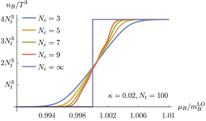
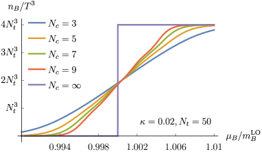
Figure 3: Onset transition to baryon condensation for different values of $N_{c}$ and $N_{\tau}$ in the strong coupling limit.

Of particular interest is the behaviour of the onset transition to finite baryon density, which is shown in Fig. 3 for different choices of $N_{c}$. We observe a steepening of the transition with increasing $N_{c}$, which asymptotically ends up in a step function, i.e. a first-order transition, even though we started with a smooth crossover at $N_{c}=3$.

Decreasing the values of $N_{\tau}$, i.e. increasing the temperature, flattens the curves with fixed $N_{c}$, but for asymptotically large $N_{c}$ a step function is obtained for any finite starting value of $N_{\tau}$. Thus, growing $N_{c}$ appears to make the onset transition to baryon matter always first-order. (With increasing temperature one may question the neglect of $\lambda_{1},\bar{h}_{1}$. Their inclusion is discussed in sections 3.6, 3.7.)

Note that, in the limit of infinite $N_{c}$, the transition is between the vacuum and a saturated lattice, similar to what happens in the static strong coupling limit at finite $N_{c}$. This saturated state is a discretisation artefact and will move towards infinity as the continuum is approached, as we discuss in section 3.8.

3.4 Thermodynamic functions for large $N_{c}$

Since we have an explicit formula for the free energy for general $N_{c}$, one can easily obtain the asymptotic behaviour of thermodynamic observables for large $N_{c}$. We study the behaviour of the different orders in the hopping expansion separately. This is necessary because, beyond the onset of baryon condensation, the leading static term represents lattice saturation, which is an unphysical artefact of discretisation. As discussed in section 2.3, correction terms do not contribute to saturation, but modify the shape of the curves as they enter their low and high density asymptotes. These effects will remain after continuum extrapolation and thus are physically significant.

The general strategy for the asymptotic analysis is most easily illustrated for the leading order contribution to the pressure at $N_{f}=1$

$$a^{4}p_{\mathrm{LO}}=\frac{1}{N_{\tau}}\ln\left(1+(N_{c}+1)h_{1}^{N_{c}}+h_{1}^{2N_{c}}\right).$$ (53)

Note that, just like in the $SU(3)$ case in (23), the prefactors before $h_{1}^{N_{c}}$ can be understood from spin-degeneracy. Specifically, a colour neutral state consisting of $N_{c}$ fermions is antisymmetric in colour space under particle exchange. The only completely symmetric spin state of $N_{c}$ spin $1/2$-particles is that with $s=N_{c}/2$ . States with this spin and spin components $-N_{c}/2\leq s_{3}\leq N_{c}/2$ are degenerate, explaining the $N_{c}+1$ prefactor.

When $h_{1}<1$ then the term $h_{1}^{N_{c}}$ is strongly suppressed (stronger than $N_{c}^{k}$ can grow for any $k$) and a Taylor expansion around $h_{1}^{N_{c}}=0$ gives

$$a^{4}p_{\mathrm{LO}} =\frac{1}{N_{\tau}}(N_{c}+1)h_{1}^{N_{c}}+\mathcal{O}(h_{1}^{2N_{c}})$$ (54)

$$\sim\frac{1}{N_{\tau}}N_{c}h_{1}^{N_{c}}\text{ for }N_{c}\rightarrow\infty.$$ (55)

For $h_{1}>1$ the term with the highest power of $h_{1}^{N_{c}}$ determines the asymptotic behaviour and one obtains

$$a^{4}p_{\mathrm{LO}} \sim\frac{1}{N_{\tau}}\ln\left(h_{1}^{2N_{c}}\right)$$ (56)

$$\sim\frac{2}{N_{\tau}}\ln(h_{1})N_{c}.$$ (57)

For higher $N_{f}$ and higher orders the terms become more complicated, but the general behaviour stays the same. For $N_{f}=2$ our findings on both sides of the onset transition are summarised in Table 1. A clear picture emerges: for $h_{1}<1$ all terms, due to the static determinant as well as the corrections, come with a factor $h_{1}^{N_{c}}$ to some power. Since the fugacity contains $m_{B}^{\mathrm{LO}}/(N_{c}T)$ in the exponential, this factor will for low temperatures always dominate the powers of $N_{c}$ and result in a stronger exponential suppression before the onset transition. In other words, the curves for all quantities will be squeezed ever more tightly against the chemical potential axis as $N_{c}$ gets large. Since we do not know the hopping expansion of the baryon mass for general $N_{c}$, we expressed our results in units of the leading order expression (20), which is responsible for onset happening at $m_{B}^{\mathrm{LO}}=\mu_{B}$ at large $N_{c}$.

The more interesting situation is $h_{1}>1$, where we first focus on the baryon number density. As explained in Section 2.3, the leading order contribution in the hopping expansion corresponds to the static determinant only, for which the onset to baryon matter is a first-order step function. This remains true for large $N_{c}$, with the lattice quark saturation density going as $a^{3}n^{\mathrm{sat}}=2N_{f}N_{c}$, i.e. the baryon density behaves as $a^{3}n_{B}^{\mathrm{sat}}\sim\mathrm{const.}$.

Order hopping expansion		$\kappa^{0}$	$\kappa^{2}$	$\kappa^{4}$
$h_{1}<1$	$a^{4}p$	$\sim\frac{1}{6N_{\tau}}N_{c}^{3}h_{1}^{N_{c}}$	$\sim-\frac{1}{48}N_{c}^{7}h_{1}^{2N_{c}}$	$\sim\frac{3N_{\tau}\kappa^{4}}{800}N_{c}^{8}h_{1}^{2N_{c}}$
	$a^{3}n_{B}$	$\sim\frac{1}{6}N_{c}^{3}h_{1}^{N_{c}}$	$\sim-\frac{N_{\tau}}{24}N_{c}^{7}h_{1}^{2N_{c}}$	$\sim\frac{(9N_{\tau}+1)N_{\tau}}{1200}N_{c}^{8}h_{1}^{2N_{c}}$
	$a^{4}e$	$\sim-\frac{\ln(2\kappa)}{6}N_{c}^{4}h_{1}^{N_{c}}$	$\sim\frac{N_{\tau}\ln(2\kappa)}{48}N_{c}^{8}h_{1}^{2N_{c}}$
	$\epsilon$	0	$\sim-\frac{1}{4}N_{c}^{3}h_{1}^{N_{c}}$
$h_{1}>1$	$a^{4}p$	$\sim\frac{4\ln(h_{1})}{N_{\tau}}N_{c}$	$\sim-12N_{c}$	$\sim 198N_{c}$
	$a^{3}n_{B}$	$\sim 4$	$\sim-N_{\tau}\frac{N_{c}^{4}}{h_{1}^{N_{c}}}$	$\sim-\frac{(59N_{\tau}-19)N_{\tau}}{20}\frac{N_{c}^{5}}{h_{1}^{N_{c}}}$
	$a^{4}e$	$\sim-4\ln(2\kappa)N_{c}$	$\sim 24\ln(2\kappa)N_{c}$
	$\epsilon$	0	$\sim-6$

Table 1: Large $N_{c}$ behaviour of the thermodynamic functions and the interaction energy per baryon, order by order in the hopping expansion, on both sides of the onset transition for $N_{f}=2$.

The most intriguing result of this section is the $N_{c}$-scaling of the pressure beyond baryon onset, $p\sim N_{c}$. Preliminary results based on leading and next-to-leading order were reported in scheunert . Stability of this finding through three orders suggests it to hold to any order in the hopping expansion, and thus for all current quark masses. In this case strongly coupled QCD beyond the onset transition to baryon matter satisfies the definition of quarkyonic matter quarky . Note that there is a finite interaction energy per baryon in units of baryon mass also for $N_{c}\rightarrow\infty$, as was conjectured in quarky . Its value at leading order $\kappa^{2}$ is determined by $d(d+1)/2$, where $d$ refers to the number of spatial dimensions.

3.5 The transition region

The results in the previous section were obtained by first fixing $h_{1}$, i.e. fixing the quark chemical potential, and then considering the limit $N_{c}\rightarrow\infty$. Right around the onset transition one can also consider $h_{1}^{N_{c}}\sim 1$. According to equation (18), this means that the quark chemical potential is adjusted such that $\mu-m\sim 1/N_{c}$, where $am=\ln(2\kappa)$ is again the leading order constituent quark mass. In this regime, the asymptotic behaviour is dominated by the prefactors of the powers of $h_{1}^{N_{c}}$, which are polynomials in $N_{c}$, see equations (41), (42), (43) and (46). For large $N_{c}$ one then obtains for the pressure in the hopping expansion

$$a^{4}p\sim\frac{4}{N_{\tau}}\ln(N_{c})-3\kappa^{2}N_{c}+\frac{(N_{\tau}-286)\kappa^{4}}{150}N_{c}^{2}+\mathcal{O}(\kappa^{6}).$$ (58)

This indicates that the hopping expansion does not converge for large $N_{c}$. In Fig. 3 this shows up by the formation of uncontrolled wiggles in the central region for sufficiently large $N_{c}$ (a first indication of this is seen for $N_{c}=9$). Thus, we cannot make a statement about the large $N_{c}$ behaviour in this window of parameter space. Fortunately, the width of this region shrinks to zero for large $N_{c}$ and does not affect the observations in the previous sections. (For the same reason, it is not clear to us whether this behaviour is related to a phase transition in $N_{c}$, as conjectured in lott ).

3.6 Inclusion of $\bar{h}_{1}$-corrections

For statements at higher temperatures, or lower $N_{\tau}$, we also need to consider what happens when $\bar{h}_{1}$ is included. In this case terms appear which mix $h_{1}$ and $\bar{h}_{1}$. For $h_{1}>1$ the large $N_{c}$ analysis is clearly unchanged, since in this case the highest powers of $h_{1}^{N_{c}}$ determine the asymptotic behaviour. For $h_{1}<1$ $\mu$-independent terms with equal power of $h_{1}$ and $\bar{h}_{1}$ become relevant as they are not suppressed when $N_{c}\rightarrow\infty$. However, these contributions are of mesonic nature and expected to scale as $\sim N_{c}^{0}$.

This can be shown explicitly for $N_{f}=1$ at leading order in the hopping expansion, as the contribution of the static determinant is known to be Unger:2014oga

$$\begin{split}-f_{h_{1},\bar{h}_{1}}&=\ln\biggl{(}\;\sum_{k=0}^{2N_{c}}T(k)(2\kappa)^{2kN_{\tau}}\\ &\qquad+\sum_{k=0}^{N_{c}}P(k)(2\kappa)^{(2k+N_{c})N_{\tau}}2\cosh(N_{c}\mu/T)+(2\kappa)^{2N_{c}N_{\tau}}2\cosh(2N_{c}\mu/T)\biggr{)}\;,\end{split}$$ (59)

with $T(k)=\binom{\min(k,2N_{c}-k)+3}{3}$ and $P(k)=(N_{c}+1-k)(k+1)$. For $\mu<a\ln(2\kappa)$ (i. e. $h_{1}<1$) the $\mu$-dependent terms vanish as $N_{c}\rightarrow\infty$. Obviously, this is not the case for the $\mu$-independent terms. Their contribution can be evaluated for $N_{c}\rightarrow\infty$ by using the following variant of the geometric series (which can be obtained by differentiation):

$$\sum_{k=0}^{\infty}(k+l)^{\underline{l}}x^{k}=\frac{l!}{(1-x)^{l}}\text{ for }\lvert x\rvert<1.$$ (60)

This results for $N_{c}\rightarrow\infty$ in the pressure

$$a^{4}p_{h_{1},\bar{h}_{1}}=-\frac{4}{N_{\tau}}\ln\left(1-(2\kappa)^{2N_{\tau}}\right)\sim N_{c}^{0}.$$ (61)

3.7 Gauge corrections and ’tHooft scaling

Our discussion so far has been for the strong coupling limit $\beta=0$, and so does not correspond to the intended ’t Hooft limit of large $N_{c}$. In this section we argue that our observations carry over to the t’Hooft limit once we include gauge corrections, at least to the orders considered.

Including the leading gauge corrections to the fermion determinant, as well as partial resummation of the corresponding diagrams to all orders, proceeds in the same manner as in bind for any $N_{c}$. Through $\mathcal{O}(\kappa^{2})$ the free energy density now reads

$$-f=\ln(z_{0}(h_{1}))+\frac{\kappa^{2}N_{\tau}}{N_{c}}\left[1+2\frac{u-u^{N_{\tau}}}{1-u}\right](-6N_{f})\frac{z_{11}(h_{1})}{z_{0}(h_{1})}^{2},$$ (62)

where $u$ can be computed using (29) and $h_{1}$ now includes corrections,

$$h_{1}=(2\kappa)^{N_{\tau}}e^{a\mu N_{\tau}}\exp\left[6N_{\tau}\kappa^{2}\frac{u-u^{N_{\tau}}}{1-u}\right].$$ (63)

In taking the ’t Hooft limit, i. e. keeping $\lambda_{H}=2N_{c}^{2}/\beta$ fixed, one has for $\lambda_{H}>1$ gw ; Drouffe:1983fv

$$u(\beta)=\frac{1}{\lambda_{H}}\;.$$ (64)

Therefore, these gauge corrections only modify the asymptotic behaviour of the thermodynamic functions by a constant $\sim N_{c}^{0}$.

Furthermore, we also consider the leading order contribution from the pure gauge sector to the effective theory (the first line in equation (2.1)) with

$$\lambda_{1}=u^{N_{\tau}}\;,$$ (65)

to leading order in the character expansion. The first correction to $-f$ in equation (33) due to the inclusion of this term, combined with the centre-symmetric part of the static determinant, reads

$$-f_{\lambda_{1},h_{1}}=6\lambda_{1}\frac{z_{(01)}z_{(0\;-1)}}{z_{0}^{2}}.$$ (66)

Employing the previously outlined integration techniques one obtains

$$z_{(01)} =\sum_{p=0}^{2N_{f}}\det_{1\leq i,j\leq N_{c}}\left(\binom{2N_{f}}{i-j+p}\right)\frac{pN_{c}}{N_{c}+2N_{f}-p}h_{1}^{pN_{c}}\;,$$ (67)

$$z_{(0\;-1)} =\sum_{p=0}^{2N_{f}}\det_{1\leq i,j\leq N_{c}}\left(\binom{2N_{f}}{i-j+p}\right)\frac{(2N_{f}-p)N_{c}}{N_{c}+p}h_{1}^{pN_{c}}\;.$$ (68)

In the ’t Hooft limit $\lambda_{1}=\frac{1}{\lambda_{H}^{N_{t}}}$, and therefore the asymptotic analysis of this term can be done in the same way as for the strong coupling contributions. The result is

$$a^{4}p_{\lambda_{1},h_{1}}\sim\frac{4}{N_{\tau}\lambda_{H}^{N_{\tau}}}N_{c}^{3}\begin{cases}h_{1}^{N_{c}},&\text{ if }h_{1}<1\;,\\ \frac{1}{h_{1}^{N_{c}}},&\text{ if }h_{1}>1\;.\end{cases}$$ (69)

Hence, the $N_{c}$ scaling of these corrections is subleading for $h_{1}>1$, while for $h_{1}<1$ the previous results are again only modified by a constant $\sim N_{c}^{0}$. Starting at $\mathcal{O}(\lambda_{1}^{4})$ there are contributions which are entirely due to the pure gauge part of the action. For these contributions only integrals of the type

$$\int\limits_{SU(N_{c})}dW{\rm Tr}(W)^{n}{\rm Tr}(W^{\dagger})^{n}=n!\quad\text{ for }\quad n\leq N_{c}$$ (70)

are relevant. When taking the large $N_{c}$ limit, order by order these contributions to the pressure are $\mu$-independent and scale as $\sim\lambda_{1}^{k}\sim N_{c}^{0}$.

The last statement hinges on the fact that the $N_{c}$ dependence of $\lambda_{1}$ is solely determined by $u$. In myers corrections to $\lambda_{1}$ to $\mathcal{O}(u^{8})$ were computed and, although some corrections do introduce additional $N_{c}$ factors, those cancel order by order when all corrections are summed up. A similar observation, including higher representations, was made in p_nc in the context of a strong coupling expansion of pure gauge theory without using an effective theory.

The influence of the gauge corrections is illustrated in Fig. 4 for two different choices of the ’t Hooft coupling. Clearly, the small quantitative modifications by the gauge corrections do not alter the qualitative $N_{c}$-behaviour observed earlier. Of course, in higher orders the situation might be more complicated, as new interactions can arise in the effective theory with non-trivial $N_{c}$-dependence. Nevertheless, the dominant contribution to the large $N_{c}$ limit of baryon dynamics should always be represented by powers of $h^{N_{c}}$ like in the leading contributions considered here, since $N_{c}$ occurs in the exponent in these cases.

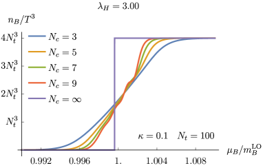
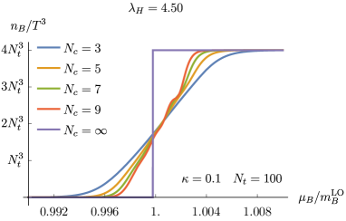
Figure 4: Baryon density, including gauge corrections, for growing $N_{c}$ with the ’t Hooft coupling held fixed. The qualitative behaviour is the same as in the strong coupling limit.

3.8 Approaching the continuum

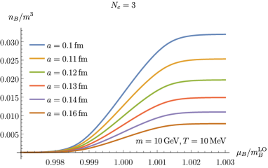
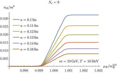
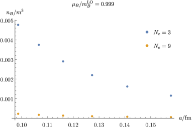
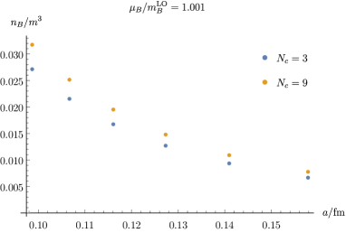
Figure 5: Continuum approach of the onset transition: steepening of the transition with growing $N_{c}$ is also obtained if the continuum limit is taken first.

This situation leaves, however, one caveat. Even if one would be able to include gauge contributions to all orders, the interchange of the $N_{c}\rightarrow\infty$ limit and the strong coupling expansion was observed to be “highly suspicious” in the case of QCD in 1+1 dimensions gw . Our analysis so far was based on taking $N_{c}$ large before a continuum limit. The fact that the density at the onset transition immediately jumps to lattice saturation indeed suggests that the limits should be taken in the opposite order, if one is interested in continuum physics. In this case, the interplay between large $N_{c}$ and the Pauli principle should lead to a finite continuum density, just as for $N_{c}=3$.

To get an idea if our results are consistent with this expectation we investigated the behaviour of the baryon density towards the continuum. To set the scale at $SU(3)$ we use the same strategy as in bind , which gives a rough estimate of the parameter space. At first, since heavy quarks have little influence on the running of the coupling, we use the non-perturbative beta-function of pure gauge theory to get a relation between $\beta_{SU(3)}$ and $a/r_{0}$, where $r_{0}$ is the Sommer parameter Necco:2001xg . Using $r_{0}=0.5$ fm sets a physical scale for the lattices and the temperature can be adjusted by $N_{\tau}$ via $T=1/(aN_{\tau})$. To obtain the corresponding $\beta$ for $SU(N_{c})$ we keep $\lambda_{H}=2N_{c}^{2}/\beta_{SU(N_{c})}=18/\beta_{SU(3)}$ fixed. Finally, the leading order expression (20) is used to keep the constituent quark mass constant for different $a$.

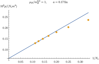
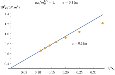
Figure 6: The $N_{c}$-scaling of the pressure, $p\sim N_{c}(1+{\rm const.\;}N_{c}^{-1}+\ldots)$, for two different lattice spacings in the interval $N_{c}\in[3,9]$.

The outcome of this procedure is illustrated in Fig. 5, where the lattice spacing is varied for fixed $N_{c}=3,9$. Each continuum extrapolation leads to a finite value for the density, which is smaller or larger, for $h_{1}<1$, $h_{1}>1$, respectively, as $N_{c}$ is increased. It is thus apparent that the transition steepens with growing $N_{c}$ also when the continuum is approached first. Similarly, the pressure is shown in Fig. 6 for two different lattice spacings and $N_{c}\in[3,9]$. Since this is far from the large $N_{c}$ limit, we explicitly checked that the first subleading contribution goes as $\sim N_{c}^{0}$. The figure shows that the full result follows the predicted $N_{c}$-scaling to hold in a region where the lattice is only about half filled, i.e., not yet dominated by lattice saturation. This behaviour appears to be stable as the lattice is made finer. While for $N_{c}=3$ and sufficiently heavy quarks a continuum limit can be explicitly taken bind ; k8 , for large $N_{c}$ this is difficult in practice, because in the problematic transition region, cf. section 3.5, the required length of the hopping series grows exponentially with $N_{c}$. We are therefore unable to explicitly demonstrate first-order behaviour or the scaling $p\sim N_{c}$ of the large $N_{c}$-limit in the continuum.

3.9 The phase diagram with growing $N_{c}$

We have seen that, in the strong coupling limit, the onset transition to baryon matter becomes first-order for any temperature. In the last section we provided evidence for a steepening of the liquid gas transition with $N_{c}$ also in the continuum. While we are unable to take the continuum and large $N_{c}$ limits in this order, we now argue on physical grounds that the onset transition has to become first order when $N_{c}\rightarrow\infty$. Within the effective theory (as well as physical QCD), the endpoint of the nuclear liquid gas transition is located where the temperature starts to exceed the binding energy per baryon. In table 1, we found the interaction energy in units of baryon mass to scale as $\epsilon\sim\mathrm{const}$. Consequently, the binding energy in $N_{c}$-independent units scales as $\sim N_{c}$ as expected, and the critical endpoint of the liquid gas transition moves to ever larger temperatures. On the other hand, the deconfinement transition temperature $T_{d}$ is only sensitive to meson physics, and in the large $N_{c}$-limit is within $\sim N_{c}^{-2}$ of its value at $N_{c}=3$ teper . Hence, in the limit $N_{c}\rightarrow\infty$, temperatures in the range $0<T<T_{d}$ never exceed the binding energy between baryons and the onset transition must be of first order.

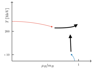
Figure 7: Arrows indicate the smooth change of the phase transition lines with growing $N_{c}$.

This implies that the critical endpoint of the baryon onset transition increases with growing $N_{c}$ until it hits another discontinuity, as indicated in Fig. 3 (right). We know already from perturbation theory that also the deconfinement transition line “straightens out” with growing $N_{c}$, as the deconfinement transition becomes less and less sensitive to the quark contributions. Altogether, we then observe how the predicted rectangular phase diagram of Fig. 2 emerges continuously by increasing $N_{c}$, as indicated in Fig. 7 .

3.10 Quarkyonic matter on the lattice?

While lattice saturation is a mere discretisation artefact and may seem uninteresting from a continuum perspective, it adds an intriguing feature here. The lattice saturation density is clearly determined by the quark degrees of freedom. Besides counting degrees of freedom, this follows also from the fact that the saturation density is precisely the same in the case of large isospin chemical potential bind . Thus, approaching saturation, the lattice is filled with quark matter.

On the other hand, the onset transitions at finite baryon as well as isospin chemical potentials are related to the condensation of hadrons, and not quarks. This follows from the fact that the critical chemical potential is different in the baryonic and isospin cases bind , i.e. $m_{B}/3\neq m_{\pi}/2$.

For increasing baryon chemical potential, a lattice filling up with baryon number is thus consistent with the picture of quarkyonic matter, in the sense that it shows a smooth transition from baryon matter to quark matter in a remarkably narrow range of chemical potentials. As the lattice is made finer, the saturation level in physical units increases and is reached at larger chemical potentials. Eventually, in the continuum limit, the interplay between the attractive baryon interaction and Pauli repulsion will lead to the physical saturation density known from nuclear matter, while the quark matter observed at lattice saturation gets shifted to larger chemical potentials (possibly infinite), with a quarkyonic regime in between.

4 Conclusions

We have studied the large $N_{c}$-behaviour of QCD in the cold and dense regime within an effective lattice theory derived by combined strong coupling and hopping expansions, which is valid for sufficiently heavy quarks. At low temperatures and $\mu_{B}\sim m_{B}$ it exhibits a transition to baryon condensation, which is the heavy quark analogue of the nuclear liquid gas transition. By considering the effective theory for general gauge group $SU(N_{c})$ we have shown that, in the strong coupling limit and through three consecutive orders in the hopping expansion, the pressure in the baryon condensed phase scales as $p\sim N_{c}$ and the onset transition becomes first-order for large $N_{c}$. This behaviour is stable under inclusion of the leading gauge corrections. We have pointed out that the continuum limit has to be taken before the large $N_{c}$ limit, which makes definite conclusions for continuum physics much harder to reach. Nevertheless, we have shown our findings to be stable also in this ordering for the range of lattice spacings and $N_{c}$-values we were able to consider with our truncated series. Our results are thus consistent with the large $N_{c}$ phase diagram and the definition of quarkyonic matter proposed in quarky .

For $N_{c}=3$, onset to baryon matter happens at $\mu_{B}^{c}<m_{B}$ (because of the binding energy between baryons) whereas $h_{1}=1$ at some $\mu_{B}>m_{B}$. The onset transition then marks the condensation of baryons, which smoothly turn into quarkyonic matter, whose pressure scales as $p\sim N_{c}$ and whose effective degrees of freedom can in principle change smoothly from baryon-like to quark-like as a function of chemical potential.

The QCD parameter values realised by nature are $m_{u,d}\sim 2-5$ MeV, in contrast to the heavy quarks on which our analysis above is based. What can be said about the physical situation? As remarked in section 3, the large $N_{c}$ analysis is independent of the current quark masses, with $m_{B}\sim N_{c}$ always and Feynman diagrams with quark loops suppressed. Thus, whether there is a deconfinement transition, a chiral transition or a crossover at $N_{c}=3$ is immaterial for the forming of a first-order horizontal deconfinement line at large $N_{c}$. On the other hand, the baryon onset transition is also present in a different effective lattice theory derived from QCD, which is valid in the chiral limit and the strong coupling regime unger . (Moreover, it is also expected from nuclear physics kapusta .) If our results generalise to all orders in the hopping expansion and are stable in the proper order of limits, then we expect the $N_{c}$-scaling of the pressure as well as the evolution of the baryon onset transition with growing $N_{c}$ to look qualitatively the same when starting from the physical situation, i.e. these would be genuine features of $SU(N_{c})$-QCD. Whether or not there is also a chiral transition at some larger chemical potential cannot be decided within the current framework, but requires additional investigations in an effective theory including chiral symmetry, such as unger .

- (1) C. Ratti, PoS LATTICE 2018 (2019) 004. doi:10.22323/1.334.0004
- (2) Y. Aoki, G. Endrodi, Z. Fodor, S. D. Katz and K. K. Szabo, Nature 443 (2006) 675 doi:10.1038/nature05120 [hep-lat/0611014].
- (3) Z. Fodor et al., Nucl. Phys. A 982 (2019) 843. doi:10.1016/j.nuclphysa.2018.12.015
- (4) A. Bazavov et al. [HotQCD Collaboration], Phys. Lett. B 795 (2019) 15 doi:10.1016/j.physletb.2019.05.013 [arXiv:1812.08235 [hep-lat]].
- (5) V. Vovchenko, J. Steinheimer, O. Philipsen and H. Stoecker, Phys. Rev. D 97 (2018) no.11, 114030 doi:10.1103/PhysRevD.97.114030 [arXiv:1711.01261 [hep-ph]].
- (6) C. S. Fischer, arXiv:1810.12938 [hep-ph].
- (7) F. Rennecke, W. j. Fu and J. M. Pawlowski, arXiv:1907.08179 [hep-ph].
- (8) M. Fromm, J. Langelage, S. Lottini and O. Philipsen, JHEP 1201 (2012) 042 doi:10.1007/JHEP01(2012)042 [arXiv:1111.4953 [hep-lat]].
- (9) L. McLerran and R. D. Pisarski, Nucl. Phys. A 796 (2007) 83 doi:10.1016/j.nuclphysa.2007.08.013 [arXiv:0706.2191 [hep-ph]].
- (10) A. Andronic et al., Nucl. Phys. A 837 (2010) 65 doi:10.1016/j.nuclphysa.2010.02.005 [arXiv:0911.4806 [hep-ph]].
- (11) T. Kojo, Y. Hidaka, L. McLerran and R. D. Pisarski, Nucl. Phys. A 843 (2010) 37 doi:10.1016/j.nuclphysa.2010.05.053 [arXiv:0912.3800 [hep-ph]].
- (12) G. Torrieri, S. Vogel and S. Lottini, J. Phys. Conf. Ser. 509 (2014) 012035. doi:10.1088/1742-6596/509/1/012035
- (13) L. McLerran and S. Reddy, Phys. Rev. Lett. 122 (2019) no.12, 122701 doi:10.1103/PhysRevLett.122.122701 [arXiv:1811.12503 [nucl-th]].
- (14) G. Torrieri, S. Lottini, I. Mishustin and P. Nicolini, Acta Phys. Polon. Supp. 5 (2012) 897 doi:10.5506/APhysPolBSupp.5.897 [arXiv:1110.6219 [nucl-th]].
- (15) C. Wozar, T. Kaestner, A. Wipf and T. Heinzl, Phys. Rev. D 76, 085004 (2007) [arXiv:0704.2570 [hep-lat]].
- (16) J. Greensite and K. Langfeld, Phys. Rev. D 88, 074503 (2013) [arXiv:1305.0048 [hep-lat]].
- (17) J. Greensite and K. Langfeld, Phys. Rev. D 90, 014507 (2014) [arXiv:1403.5844 [hep-lat]].
- (18) G. Bergner, J. Langelage and O. Philipsen, JHEP 1511, 010 (2015) [arXiv:1505.01021 [hep-lat]].
- (19) I. Montvay and G. Münster, “Quantum fields on a lattice”, Cambridge University Press 1994, doi:10.1017/CBO9780511470783
- (20) J. Langelage, G. Münster and O. Philipsen, JHEP 0807, 036 (2008) [arXiv:0805.1163 [hep-lat]].
- (21) J. Langelage and O. Philipsen, JHEP 1001, 089 (2010) [arXiv:0911.2577 [hep-lat]].
- (22) J. Langelage and O. Philipsen, JHEP 1004 (2010) 055 doi:10.1007/JHEP04(2010)055 [arXiv:1002.1507 [hep-lat]].
- (23) B. Svetitsky and L. G. Yaffe, Nucl. Phys. B 210 (1982) 423. doi:10.1016/0550-3213(82)90172-9
- (24) J. Polonyi and K. Szlachanyi, Phys. Lett. 110B (1982) 395. doi:10.1016/0370-2693(82)91280-1
- (25) J. Langelage, S. Lottini and O. Philipsen, JHEP 1102, 057 (2011) [JHEP 1107, 014 (2011)] [arXiv:1010.0951 [hep-lat]].
- (26) T. C. Blum, J. E. Hetrick and D. Toussaint, Phys. Rev. Lett. 76 (1996) 1019 doi:10.1103/PhysRevLett.76.1019 [hep-lat/9509002].
- (27) J. Langelage, M. Neuman and O. Philipsen, JHEP 1409, 131 (2014) [arXiv:1403.4162 [hep-lat]].
- (28) J. Hoek, N. Kawamoto and J. Smit, Nucl. Phys. B 199 (1982) 495. doi:10.1016/0550-3213(82)90357-1
- (29) J. Glesaaen, M. Neuman and O. Philipsen, JHEP 1603, 100 (2016) [arXiv:1512.05195 [hep-lat]].
- (30) P. M. Lo, B. Friman and K. Redlich, Phys. Rev. D 90, no. 7, 074035 (2014) [arXiv:1406.4050 [hep-ph]].
- (31) C. S. Fischer, J. Luecker and J. M. Pawlowski, Phys. Rev. D 91, no. 1, 014024 (2015) [arXiv:1409.8462 [hep-ph]].
- (32) M. Fromm, J. Langelage, S. Lottini, M. Neuman and O. Philipsen, Phys. Rev. Lett. 110 no. 12, 122001 (2013) [arXiv:1207.3005 [hep-lat]].
- (33) T. D. Cohen, Phys. Rev. Lett. 91, 222001 (2003) doi:10.1103/PhysRevLett.91.222001 [hep-ph/0307089].
- (34) P. Adhikari and T. D. Cohen, Phys. Rev. C 88 (2013) no.5, 055202 doi:10.1103/PhysRevC.88.055202 [arXiv:1307.7725 [nucl-th]].
- (35) T. D. Cohen, N. Kumar and K. K. Ndousse, Phys. Rev. C 84 (2011) 015204 doi:10.1103/PhysRevC.84.015204 [arXiv:1102.2197 [nucl-th]].
- (36) G. ’t Hooft, Nucl. Phys. B 72 (1974) 461. doi:10.1016/0550-3213(74)90154-0
- (37) E. Witten, Nucl. Phys. B 160 (1979) 57. doi:10.1016/0550-3213(79)90232-3
- (38) S. Borsanyi, Z. Fodor, C. Hoelbling, S. D. Katz, S. Krieg and K. K. Szabo, Phys. Lett. B 730 (2014) 99 doi:10.1016/j.physletb.2014.01.007 [arXiv:1309.5258 [hep-lat]].
- (39) A. Bazavov et al. [HotQCD Collaboration], Phys. Rev. D 90 (2014) 094503 doi:10.1103/PhysRevD.90.094503 [arXiv:1407.6387 [hep-lat]].
- (40) P. Scior and L. von Smekal, Phys. Rev. D 92 (2015) no.9, 094504 doi:10.1103/PhysRevD.92.094504 [arXiv:1508.00431 [hep-lat]].
- (41) A. S. Christensen, J. C. Myers and P. D. Pedersen, JHEP 1402 (2014) 028 doi:10.1007/JHEP02(2014)028 [arXiv:1312.3519 [hep-lat]].
- (42) J. M. Drouffe and J. B. Zuber, Phys. Rept. 102, 1 (1983). doi:10.1016/0370-1573(83)90034-0
- (43) F. Green and S. Samuel, Nucl. Phys. B 190 (1981) 113. doi:10.1016/0550-3213(81)90486-7
- (44) D. J. Gross and E. Witten, Phys. Rev. D 21 (1980) 446. doi:10.1103/PhysRevD.21.446
- (45) Y. Nishida, Phys. Rev. D 69 (2004) 094501 doi:10.1103/PhysRevD.69.094501 [hep-ph/0312371].
- (46) C. Krattenthaler, Séminaire Lotharingien Combin. 42 (1999) (The Andrews Festschrift), paper B42q, 67 pp [arXiv:9902004 [math.co]]
- (47) O. Philipsen and J. Scheunert, arXiv:1812.02014 [hep-lat].
- (48) S. Lottini and G. Torrieri, Phys. Rev. Lett. 107 (2011) 152301 doi:10.1103/PhysRevLett.107.152301 [arXiv:1103.4824 [nucl-th]].
- (49) W. Unger, PoS LATTICE 2014 (2014) 192 doi:10.22323/1.214.0192 [arXiv:1411.4493 [hep-lat]].
- (50) S. Necco and R. Sommer, Nucl. Phys. B 622 (2002) 328 doi:10.1016/S0550-3213(01)00582-X [hep-lat/0108008].
- (51) B. Lucini, M. Teper and U. Wenger, JHEP 0401 (2004) 061 doi:10.1088/1126-6708/2004/01/061 [hep-lat/0307017].
- (52) P. de Forcrand, J. Langelage, O. Philipsen and W. Unger, Phys. Rev. Lett. 113 (2014) no.15, 152002 doi:10.1103/PhysRevLett.113.152002 [arXiv:1406.4397 [hep-lat]].
- (53) J. I. Kapusta and C. Gale, “Finite-temperature field theory: Principles and applications,” Cambridge University Press 2006, doi:10.1017/CBO9780511535130