Searching for ultralight bosons with spin measurements of a population of binary black hole mergers

Abstract

Ultralight bosons can form clouds around rotating black holes if their Compton wavelength is comparable to the black hole size. The boson cloud spins down the black hole through a process called superradiance, lowering the black hole spin to a characteristic spin determined by the boson mass and the black hole mass. It has been suggested that spin measurements of the black holes detected by ground-based gravitational-wave detectors can be used to constrain the mass of ultralight bosons. Unfortunately, a measurement of the individual black hole spins is often uncertain, resulting in inconclusive results. Instead, we use hierarchical Bayesian inference to combine information from multiple gravitational-wave sources and to obtain stronger constraints. We show that hundreds of high signal-to-noise ratio gravitational-wave detections are enough to exclude (confirm) the existence of noninteracting bosons in the mass range $\left[10^{-13},3\times 10^{-12}\right]$ eV $\left([10^{-13},10^{-12}]~{}\rm{eV}\right)$. The precise number depends on the distribution of black hole spins at formation and the mass of the boson.

I Introduction

Ultralight bosons with masses $\lesssim 10^{-11}\,\mathrm{eV}$, including axionlike particles [1, 2, 3], dilatons and, moduli [4, 5, 6] and fuzzy dark matter [7, 8, 9, 10, 11], have been proposed as a potential solution to various problems ranging from fundamental physics to cosmology [12, 2, 3, 13, 14, 15, 6, 16, 17, 18, 19, 20, 21]. Efforts are underway to search for these ultralight bosons using table-top experiments or astronomical observations [22, 23, 24, 25, 26, 27, 28, 29, 30, 31, 32, 33, 34, 35, 36, 37, 38, 39, 40, 41, 42, 43, 44, 45, 46, 47, 48, 49, 50, 51, 52, 53]. When the Compton wavelength of the hypothetical boson is comparable to the size of a black hole (BH), i.e., $\alpha\equiv GM\mu_{s}/\hbar c^{3}\sim 1$, where $\alpha$ is the “gravitational fine-structure constant”, $M$ is the BH mass and $\mu_{s}$ is the boson mass, then a classical wave amplification process (superradiance) forms a bosonic cloud around the BH [54, 55, 56, 57, 58, 6, 17, 59, 60]. The formation of this cloud extracts rotational energy from the BH until the BH reaches a critical spin set by the Compton frequency of the boson and the mass of the BH [58, 6, 17, 59, 60]. This results on a critical spin curve on the BH mass-spin plane (e.g. Fig. 3 of Ref [17]): BHs born with spins above the critical spin curve will rapidly spin down until their final masses and spins lie on the curve. The net result of the superradiance process is thus to carve a region of the mass-spin plane, above the critical spin curve, where BHs are unlikely to be observed (“exclusion region”). Since the exact position and extent of the exclusion region depend on the boson mass (again, Fig. 3 of Ref [17]), one can use mass and spin measurements for a population of BHs to search and characterize ultralight bosons (e.g. [6, 17, 34, 35, 36, 46]).

Spin measurements of BHs in X-ray binaries (see e.g. References [61, 62]) could be used to search for bosons with their masses commensurate with BHs in the mass range $5~{}\mathrm{M}_{\odot}<M\lesssim 20~{}\mathrm{M}_{\odot}$ [61, 63]. Gravitational-wave (GW) signals emitted by binary black holes (BBHs) provide another avenue, as they encode the properties of their sources, including the masses and spins of the two component BHs. Since ground-based GW detectors such as LIGO and Virgo [64, 65] can detect heavier BHs ($M$ up to $\sim 100~{}\rm{M}_{\odot})$ [66, 67] than those found in X-ray binaries, the spin measurements inferred from GWs probe a lighter range of boson mass. This probe is complicated by two facts: (i) the measurements of individual BH spins with ground-based GW detectors are usually challenging [68, 69, 70, 71] and (ii) what is measured is the distribution of spins at merger, which is not only impacted by an eventual interaction with the bosons, but also on the distribution of spins at birth [72, 73, 74, 75].

In this paper we perform hierarchical Bayesian inference on a population of BBHs, to simultaneously infer the boson mass and the BH spin distribution at formation [76, 77, 78, 79, 80, 81, 82, 83, 84]. First, we show that the existence of ultralight bosons in the mass range between $10^{-13}$ eV and $3\times 10^{-12}~{}\mathrm{eV}$ can be ruled out with $\mathcal{O}(100)$ high signal-to-noise ratio (SNR) BBH detections.  Second, we illustrate how our method can confirm the existence of bosons with two examples of boson masses, $\mu_{s}=10^{-12}$ and $10^{-13}$ eV.

II Critical spin arising from superradiant instability

GW measurements yield the masses and spins of BHs at the time of merger. Therefore, one needs to account for the impact of superradiance on the evolution of spins, which we quickly review here. Superradiance causes the growth of a boson cloud in a time scale $\tau^{\rm inst}_{[nlm]}$, called instability time scale, and eventually spins down the host BH to a characteristic critical spin $\chi^{\infty}_{[nlm]}$ (which will be defined below) [58, 6, 17, 60]. The indices $[nlm]$ are the analog of the hydrogen atom quantum numbers, i.e., a set of radial, orbital azimuthal, and magnetic quantum numbers, of the cloud’s bound states.  For any given $[nlm]$ mode, the instability time scale is representative of the exponential growth of the occupation number of the bosons in that mode, such that modes with small $\tau^{\rm inst}_{[nlm]}$ are populated quickly.

One often introduces the inverse of the instability time scale $\tau^{\mathrm{inst}}_{[nlm]}$, called the superradiant rate $\Gamma^{\mathrm{inst}}_{[nlm]}$, which can be analytically calculated for $\alpha\ll 1$ [85, 6, 17, 59, 60] (hereafter, we set $G=c=\hbar=1$),

$$\begin{split}\Gamma^{\mathrm{inst}}_{[nlm]}=&\mu_{s}(\mu_{s}M)^{4l+4}(m\chi-2\mu_{s}r_{+})\\ &\times\frac{2^{4l+2}(2l+1+n)!}{(l+1+n)^{2l+4}n!}\left[\frac{l!}{(2l)!(2l+1)!}\right]^{2}\\ &\times\prod_{k=1}^{l}[k^{2}(1-\chi^{2})+(m\chi-2\mu_{s}r_{+})^{2}],\end{split}$$ (1)

where $\chi$ is the dimensionless spin of the BH and $r_{+}\equiv M\left(1+\sqrt{1-\chi^{2}}\right)$ is the radial coordinate of the BH outer horizon. For the first few $l$’s, the fastest growing mode is the one with $l=m$, such that $\Gamma^{\mathrm{inst}}_{[nlm]}$ is the largest [17]. For any given $M$ and $\mu_{s}$, superradiance can happen as long as $\Gamma_{[nlm]}^{\mathrm{inst}}(\mu_{s},M,\chi)>0$; hence,

$$\frac{\alpha}{m}<\frac{\chi}{2\left(1+\sqrt{1-\chi^{2}}\right)}<\frac{1}{2}.$$ (2)

which gives a condition on the BH spin $\chi$ such that superradiance can happen for the mode $[nlm]$. If the BH-cloud system had an infinite amount of time to evolve without disturbances, the spin angular momentum of the BH would eventually be lowered to the point where Eq. (2) cannot be satisfied or, equivalently, where $\Gamma_{[nlm]}^{\mathrm{inst}}=0$ (saturation of the superradiance). The critical spin for the $[nlm]$ mode is thus defined as the spin below which the superradiant growth of the cloud of the $[nlm]$ mode is forbidden,

$$\chi^{\infty}_{[nlm]}=\frac{4\alpha m}{4\alpha^{2}+m^{2}}.$$ (3)

Besides the spin angular momentum of the BH, a small fraction $(\lesssim 10\%)$ of BH mass is also extracted and contributes to the cloud’s mass [17, 59, 86]. This is smaller or at most comparable to the BH mass uncertainty from GW measurements [70]. Therefore, we neglect the BH mass loss due to superradiance and assume that the BH masses at merger are the same as the masses at formation.

In this study, we do not allow for boson self-interaction, which would lead to additional phenomenology [17, 34, 87]. We refer to Ref. [46] for the analysis on self-interacting bosons using spin measurements of x-ray binaries.

III Postsuperradiant spin of astrophysical black holes

Astrophysical BHs in binaries have finite lifetimes, $\tau_{s}$, which implies their spins at merger will not reach the critical spin $\chi^{\infty}_{[nlm]}$. Therefore, we need to calculate the postsuperradiant BH spin for the $[nlm]$ mode, $\chi_{[nlm]}$  by solving $\Gamma^{\rm inst}_{[nlm]}(\mu_{s},M,\chi_{[nlm]})=1/\tau_{s}$ for $\chi_{[nlm]}$, i.e., we truncate the spin evolution when the instability time scale decreases to the BH lifetime.

Naturally, if the lifetime of a BH is too short compared to the time required for the boson cloud to spin down its host BH, the effect might not even be measurable. Refs. [17, 34, 35] find that the bosonic field in the cloud should increase by $\sim 180$ $e$-foldings for the cloud to store a large amount of the BH angular momentum. This $e$-folding requirement translates to a “growth time scale” for the boson cloud such that it can significantly spin down the BH, $\tau^{\rm grow}_{[nlm]}\approx 180~{}\tau^{\rm inst}_{[nlm]}(\mu_{s},M,\chi_{I[nlm]})$, where $\chi_{I[nlm]}$ is the dimensionless spin of the BH at the onset of superradiance of the $[nlm]$ mode. Therefore, a BH that is born with a spin at formation $\chi_{F}$ and merges in $\tau_{s}$ can be spun down to the postsuperradiant spin $\chi_{[nlm]}$ (which is given by the solution of $\Gamma^{\rm inst}_{[nlm]}(\mu_{s},M,\chi_{[nlm]})=1/\tau_{s}$) only if $\chi_{F}>\chi_{[nlm]}$ and $\tau_{s}>\tau^{\rm growth}_{[nlm]}$.

Multiple clouds with different modes can be excited within the lifetime of a BH. The highest mode of the cloud that can be populated is given by the condition $\tau^{\rm grow}_{[nlm]}~{}{<}~{}\tau_{s}~{}{<}~{}\tau^{\rm grow}_{[n(l+1)(m+1)]}$. One can then estimate the BH spin at merger $\chi_{M}$ to be the postsuperradiant spin of this highest mode $\chi_{[nlm]}$, given the BH spin at formation and its lifetime. For example, if a BH is born with $\chi_{F}>\chi_{[011]}$, then the formation of the initial cloud (with the time scale $\tau^{\rm grow}_{[011]}$) slows down the BH spin to $\chi_{[011]}$. After its formation, the cloud dissipates away emitting nearly monochromatic gravitational waves [17, 35, 36, 37, 88]. Next, a second (“higher mode”) cloud is formed with the time scale $\tau^{\rm grow}_{[022]}$, and the BH spins down further to the postsuperradiant spin of this next mode $\chi_{[022]}$, if $\chi_{[011]}>\chi_{[022]}$. This cycle repeats until the BBH merges at time $\tau_{s}$. In Fig. 1, we show a schematic picture of a system for which both the $l=m=1$ and the $l=m=2$ clouds have enough time to form before merger. We note that only the first few growing modes $n=0$ and $l=m\leq 3$ are relevant for the typical astrophysical time scales $\tau_{s}\lesssim 10$ Gyr.

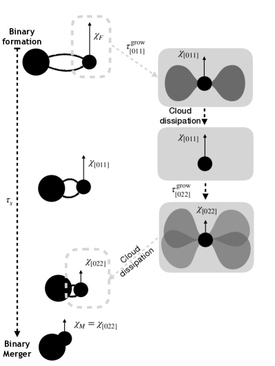
Figure 1: The possible evolution of a BBH system from its formation to merger. The cartoon follows the growth and dissipation of boson clouds around one of the BHs. The BH starts with a spin at formation $\chi_{F}$ large enough to trigger superradiant instability. The $n=0,l=m=1$ cloud forms with a characteristic time scale $\tau^{\rm grow}_{[011]}$, lowering the BH spin to $\chi_{[011]}$. The cloud is dissipated through monochromatic GW emission. In this example, the $\chi_{[011]}$ is large enough that a second cloud ($n=0,l=m=2$) is also created, and further reduces the BH spin to $\chi_{[022]}$. At this point the spin of the BH is too small to trigger the formation of higher-order clouds, and the BH will merge with spin $\chi_{M}=\chi_{[022]}$. The highest level of the cloud that can be populated depends on $\chi_{F}$ and on the inspiral time scale $\tau_{s}$. (The plot is not to scale.)

In principle, the BBH merger could cause the cloud to fall back to its host through level mixing [17, 86, 89, 90, 91]. While one could think that this results in a transfer of the cloud’s angular momentum back to the host BH, which would then be spun-up, most of the in-falling modes have nonpositive angular momentum (i.e. $m\leq 0$) due to selection rules. [89, 90, 91]. This is why recent studies have suggested that the in-falling cloud instead spins down the host BH, or might decrease the orbital angular momentum in the binary system [86, 89, 90, 92, 93, 91]. An eventual decrease in the BH spin by the fallback would further increase the size of the exclusion region on the BH mass-spin plane, making it easier to verify the existence of bosons with our method. To be conservative, we ignore this binary effect on the postsuperradiant spins.

IV Testing the Ultralight-boson Hypothesis using Hierarchical Bayesian inference

An astrophysical distribution of BH spins at birth, which produces mainly small spins in the absence of superradiance, is partially degenerate with the postsuperradiant spin distribution that originates from a moderate (or high) spin distribution at birth in the presence of superradiance.  Hence, we need to simultaneously infer the spin distribution at birth and the boson mass to properly account for this degeneracy.

We use hierarchical Bayesian inference [79, 78, 81, 82, 83], and consider two competing models: (i) in the “boson model,” $\mathcal{H}_{\mathrm{B}}$, we assume that a boson exists such that BHs can spin down to the corresponding postsuperradiant spins $\chi_{[nlm]}$ through superradiance (Sec. III); (ii) in the “astrophysical model,” $\mathcal{H}_{\rm{A}}$, ultralight bosons do not exist, and the spins of BHs merging in binaries are entirely determined by their astrophysical evolution.

The two hypotheses are distinguishable through the resulting distribution of the BH spins at merger. Specifically, for $\mathcal{H}_{\mathrm{B}}$, we assume

$$\mathcal{H}_{\mathrm{B}}:\chi_{M}=\begin{cases}\chi_{[nlm]},&\text{if }\tau^{\rm grow}_{[nlm]}<\tau_{s}<\tau^{\rm grow}_{[n(l+1)(m+1)]}\\ \chi_{F},&\text{otherwise}\end{cases}$$ (4)

where $\chi_{F}$ and $\chi_{M}$ are the individual BH spins at formation and at merger, respectively, and $\tau_{s}$ is the BH lifetime. The condition $\tau^{\rm grow}_{[nlm]}<\tau_{s}<\tau^{\rm grow}_{[n(l+1)(m+1)]}$ implies that $\chi_{[nlm]}$ is obtained as the postsuperradiance spin of the highest mode that can be populated within the binary lifetime. If superradiance does not happen for the specific BH (either because of its parameters at formation or because of the time scale to merger) then the spin at merger is the same as the spin at formation, i.e. $\chi_{M}=\chi_{F}$. On the other hand, there is no superradiance and therefore no spin evolution for $\mathcal{H}_{\rm{A}}$. Thus, for all black holes, the spin remains unchanged from formation to merger,

$$\mathcal{H}_{\rm{A}}:\chi_{M}=\chi_{F}.$$ (5)

For both models, we parametrize the distribution of BH spins at formation with a beta distribution, controlled by two unknown shape parameters $\alpha>0$ and $\beta>0$: $p(\chi_{F}|\alpha,\beta)\propto\chi_{F}^{\alpha-1}(1-\chi_{F})^{\beta-1}$. This is a generic functional form that can capture multiple different formation pathways [94, 80]. The boson model thus depends on three hyperparameters $\Lambda_{\mathcal{H}_{\mathrm{B}}}=(\alpha,\beta,\mu_{s})$, while the astrophysical model only has two hyperparameters $\Lambda_{\mathcal{H}_{\rm{A}}}=(\alpha,\beta)$. We aim at measuring the hyperparameters $\Lambda$, given a set of $N$ GW observations $\mathbf{d}=\left\{d_{k}\right\}$, whose morphology depends on a set of parameters $\theta$, such as BH masses, spins and distance [95]. The distribution of measured $\Lambda$, known as hyperposterior, can be written as [79, 78, 81, 82, 83]:

$$p(\Lambda|\mathbf{d})\propto\pi(\Lambda)\prod_{k}^{N}\left[\frac{1}{\Sigma(\Lambda)}\int p(\theta|\Lambda)p(d_{k}|\theta)d\theta\right]$$ (6)

where $p(\theta|\Lambda)$ is the expected distribution of the individual events parameters, given the hyperparameters; $\pi(\Lambda)$ are the priors of the hyperparameters; $p(d_{k}|\theta)$ is the likelihood of the $k$th GW source; and $\Sigma(\Lambda)$ is the normalization factor given by

$$\Sigma(\Lambda)=\int p(\theta|\Lambda)p_{\mathrm{det}}(\theta)d\theta,$$ (7)

where $p_{\mathrm{det}}(\theta)$ is the detection probability for a BBH with parameters $\theta$. The normalization factor $\Sigma(\Lambda)$ can thus be interpreted as the fraction of detectable BBHs.

When working with the boson model, $\Lambda_{\mathcal{H}_{\mathrm{B}}}=(\alpha,\beta,\mu_{s})$ and $\theta_{\mathcal{H}_{\mathrm{B}}}=(M_{1},M_{2},\chi_{M,1},\chi_{M,2},\tau_{s})$, where $M_{i}$ and $\chi_{M,i}$ are the masses and spins (at merger) of the two compact objects in the binary. One thus has:

$$p\left(\Lambda_{\mathcal{H}_{\mathrm{B}}}|\mathbf{d},\mathcal{H}_{\mathrm{B}}\right)\propto\pi(\Lambda_{\mathcal{H}_{\mathrm{B}}})\prod_{k}^{N}\left\{\frac{1}{\Sigma(\Lambda_{\mathcal{H}_{\mathrm{B}}})}\int p(d_{k}|\theta_{\mathcal{H}_{\mathrm{B}}})\pi(M_{1},M_{2},\tau_{s})\prod_{i=1}^{2}\left[p(\chi_{M,i}|\Lambda_{\mathcal{H}_{\mathrm{B}}},M_{i},\tau_{s})dM_{i}d\chi_{M,i}\right]d\tau_{s}\right\},$$ (8)

In this expression, $\pi(M_{1},M_{2},\tau_{s})$ is the prior on the component masses and the merger time of BBHs, $\pi(\Lambda_{\mathcal{H}_{\mathrm{B}}})$ is the prior on the hyperparameters of the model $\mathcal{H}_{\mathrm{B}}$, and $p(\chi_{M,i}|\Lambda_{\mathcal{H}_{\mathrm{B}}},M_{i},\tau_{s})$ is the distribution of the spin magnitude at merger of $\mathcal{H}_{\mathrm{B}}$. It can be derived from the spin-magnitude distribution at formation as follows:

$$\begin{split}&p(\chi_{M,i}|\alpha,\beta,\mu_{s},M_{i},\tau_{s})\\ &=\int_{0}^{1}p(\chi_{M,i}|\mu_{s},M_{i},\tau_{s},\chi_{F,i})p(\chi_{F,i}|\alpha,\beta)d\chi_{F,i},\end{split}$$ (9)

in which we define the conditional probability

$$\begin{split}&p(\chi_{M,i}|\mu_{s},M_{i},\tau_{s},\chi_{F,i})\\ &=\delta\left[\chi_{M,i}-\chi_{[nlm]}(\mu_{s},M_{i},\tau_{s},\chi_{F,i})\right]\Theta\left[\chi_{F,i}-\chi_{[nlm]}\right]\\ &+\delta(\chi_{M,i}-\chi_{F,i})\Theta\left[\chi_{[nlm]}-\chi_{F,i}\right],\end{split}$$ (10)

where $\delta[...]$ is a Dirac delta that maps from the spin at formation to the spin at merger, and $\Theta[...]$ is a Heaviside step function that enforces the superradiance condition $\chi_{F,i}>\chi_{[nlm]}$. Since the growth time scale $\tau^{\rm grow}_{[nlm]}$ depends mildly on the initial spin at the onset of the superradiance, the postsuperradiant spin $\chi_{[nlm]}$ depends on four parameters $(\mu_{s},M,\tau_{s},\chi_{F})$ in principle. One needs to calculate $\chi_{[nlm]}$ for each $\chi_{F,i}$ to precisely evaluate the integral in Eq. (9). To facilitate the evaluation of this integral during the sampling process, we simplify the dependence of $\chi_{F,i}$ in $\chi_{[nlm]}$ with the following approximations to fix the values of $\chi_{I[nlm]}$. For the dominant $[011]$ mode, we set the spin at the onset to the midpoint between the minimum spin value required for superradiance and the maximal Kerr spin: $\chi_{I[011]}\approx(1+\chi_{[011]})/2$. This is justified because the growth time scale varies by only around 1 order of magnitude for spins in the range $\chi_{I[011]}\in[\chi_{[011]},1]$. After spin-down, the BH settles on the postsuperradiant spin of the given mode, $\chi_{[nlm]}$. Therefore, we approximate the initial spin of each subsequent mode $\chi_{[n(l+1)(m+1)]}$ by the preceding mode postsuperradiant spin, i.e., $\chi_{I[n(l+1)(m+1)]}\approx\chi_{[nlm]}$. With the above simplifications, $\chi_{[nlm]}$ only depends on $(\mu_{s},M_{i},\tau_{s})$ and we can approximate Eq. (9) as

$$\begin{split}p(\chi_{M,i}|\alpha,\beta,&\mu_{s},M_{i},\tau_{s})\approx f_{\rm SR}\delta(\chi_{M,i}-\chi_{[nlm]})\\ &+p(\chi_{M,i}|\alpha,\beta)\Theta(\chi_{[nlm]}-\chi_{M,i}),\end{split}$$ (11)

with $f_{\rm SR}$ being the differential fraction of BHs that undergo superradiance at the BH mass $M_{i}$:

$$\begin{split}&f_{\rm SR}(\mu_{s},M_{i},\tau_{s},\alpha,\beta)\\ \equiv&\int_{0}^{1}p(\chi_{F,i}|\alpha,\beta)\Theta\left[\chi_{F,i}-\chi_{[nlm]}(\mu_{s},M_{i},\tau_{s})\right]d\chi_{F,i}.\end{split}$$ (12)

In the astrophysical model, $\mathcal{H}_{\rm{A}}$, one obtains a similar expression for $p(\Lambda_{\mathcal{H}_{\rm{A}}}|\mathbf{d},\mathcal{H}_{\rm{A}})$ by replacing $\mathcal{H}_{\mathrm{B}}\rightarrow\mathcal{H}_{\rm{A}}$ everywhere, and removing all references to $\tau_{s}$, which is not a relevant parameter of $\mathcal{H}_{\rm{A}}$.

While calculating Eq. (8), we use a power law prior $\pi(M_{1})\propto M_{1}^{-2.35}$ for the primary mass [96], and uniform prior for mass ratio $q=M_{2}/M_{1}$ with $M_{2}\leq M_{1}$. We also assume that $\tau_{s}$ is known (for the $\mathcal{H}_{\mathrm{B}}$ model) and fixed at $10\,\rm Myr$: $\pi(\tau_{s})=\delta(\tau_{s}-10\,{\rm Myr})$, which is toward the lower limit of the typical inspiral time scales, according to numerical simulations ($\sim 10\,{\rm Myr}-10\,{\rm Gyr})$ [97, 98, 99, 100, 101, 102, 103, 104, 105, 106, 107]. From one side, this choice is conservative as it allows for the least time for BHs to spin-down due to superradiance, making it harder to find evidence for bosons. From the other side, restricting the merger time prior overestimates the prior information thus overestimates the evidence for the boson hypothesis $\mathcal{H}_{B}$ in Eq. (8). Nevertheless, the additional parameter space in $\tau_{s}$ is expected to contribute modestly to the Bayes factor because the corrections to the available mass-spin parameter space are mostly smaller than the mass-spin measurement uncertainties. Therefore, while more realistic models for the merger time prior $\pi(\tau_{s})$ could be used, our choice is sufficient for advanced GW detectors, given their limited precision in the measurement of component masses and spins.

Since we assume the BH mass distribution is known, we do not need to consider its selection effect while calculating $\Sigma(\Lambda)$. We can also ignore selection effects due to BH spins as the expected number of observations only varies by $\lesssim 10\%$ for different spin models [76, 94, 108]. Furthermore, for $\Lambda_{B}$, the fraction of detectable BBHs does not depend on $\mu_{s}$. Based on the above arguments, we therefore assume $\Sigma(\Lambda_{\mathcal{H}_{\mathrm{B}}})$ and $\Sigma(\Lambda_{\mathcal{H}_{\rm{A}}})$ are constants in the evaluation of the hyperposteriors. In generating the simulations, however, we fully account for all selection effects so that the number of sources can be interpreted as the expected number of detections in future observations.

Integrating Eq. (8), and the equivalent expression for $\mathcal{H}_{\rm{A}}$, over the whole hyperparameters space yields evidences $Z_{\mathcal{H}_{\mathrm{B}}}$ and $Z_{\mathcal{H}_{\rm{A}}}$ that can be used to calculate the Bayes factor between the boson and astrophysical hypothesis: $\mathcal{B}_{\rm{A}}^{\rm{B}}={Z_{\mathcal{H}_{\mathrm{B}}}}/{Z_{\mathcal{H}_{\rm{A}}}}$. We also perform a Monte Carlo simulation of 50 different sets of sources in every simulated universe. This allows us to estimate the probability distribution of the Bayes factors due to Poisson fluctuation for each number of detections $N$.

V Mock data analysis

The method described above can be applied to both simulated and real detections. We first demonstrate its use on three different simulated “universes”: (i) one with a boson scalar field with $\mu_{s}=10^{-13}\,\rm eV$, (ii) one with a boson with $\mu_{s}=10^{-12}\,\rm eV$, and (iii) one where no boson exists (“astrophysical population”). To create the mock populations, we generate BBHs with component masses $M_{1,2}$ following the same prior in the model: $\pi(M_{1})\propto M_{1}^{-2.35}$, uniform distribution for $q$ in $[0.1,1]$ and require both $\{M_{1},M_{2}\}\in[5,50]\rm M_{\odot}$, consistently with Ref. [80]. The BBHs are distributed uniformly in the source-frame comoving volume, as well as the sky positions, orbital orientations and polarization angles in the unit sphere. The astrophysical processes that set the initial spin magnitude and orientation are still to be fully understood [72, 73, 74, 75]. For each of the three universes, we consider two distributions of formation spin magnitudes $\chi_{F,i}$: (a) uniform in $[0,1)$ (“flat spin”) and (b) $p(\chi_{F,i})\propto(1-\chi_{F,i})$ (“low spin”), with an isotropic spin orientation in both cases. The true shape parameters of the beta distribution are $\alpha=\beta=1$ and $\alpha=1,\beta=2$ for the “flat spin” and “low spin” populations, respectively.

When simulating the universes where bosons exist, we need to evolve the BH spins at formation to the spins at merger using Eq. (4). We assume all BBHs have a short merger time scale $\tau_{s}=10$ Myr, which minimizes the effect of superradiance and is thus a conservative choice. To keep the computational cost of the analysis reasonable, of all the sources we generate, we only analyze those for which SNR$>30$. These are the only sources that will contribute to the test since individual spins are hard to measure for low or medium SNR BBHs [68, 70]. The populations of synthetic BBH sources are thus added into simulated noise of the LIGO and Virgo detectors at design sensitivity [109, 110]. We use the LALInference [111, 112] algorithm with the IMRPhenomPv2 waveform family [113] to obtain posterior and likelihood distributions for the compact binary parameters of the simulated sources, which can be used to infer the population hyperparameters as described in the previous section. For all of the hyperparameters, we use uniform-in-log priors, with ranges $[0.01,10]$ for $\alpha$ and $\beta$, as well as $[10^{-13},3\times 10^{-12}]$ eV for $\mu_{s}$, which is the range of $\mu_{s}$ that can be realistically probed with ground-based GW detectors [17, 34, 35, 88].

In Fig. 2, we show the evolution of the log Bayes factor boson versus astrophysical model, $\log_{10}\mathcal{B}^{\rm B}_{\rm A}$ as more events are used for the test. The bottom $x$-axes show the numbers of loud events, while the top ones show the numbers of total events. 

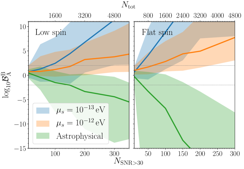
Figure 2: The $\log_{10}$ Bayes factor between the boson and astrophysical hypothesis as a function of the number of sources $N_{\rm SNR>30}$ from the boson with $\mu_{s}=10^{-13}\,\mathrm{eV}$ (blue), boson with $\mu_{s}=10^{-12}\,\mathrm{eV}$ (orange), and astrophysical (green) populations. For each population, we repeat the analysis with the low spin (left panel) and flat spin (right panel) distribution at formation. The solid lines and colored bands are medians and 90% credible intervals over 50 realizations of a population with $N_{\rm SNR>30}$ sources. The two horizontal lines show $\mathcal{B}_{\rm{A}}^{\rm{B}}=0.01$ and 100.

All curves show that the underlying hypothesis is correctly preferred by the method, given enough number of observations. In Table 1, we report the expected numbers of observations required to significantly  prefer a hypothesis for all pairs of the spin distribution and boson mass. In general, we would expect that fewer sources are required to disprove the boson hypothesis (first row of Table 1) than to confirm it. This is because even one highly spinning BH measurement can contradict $\mathcal{H}_{\mathrm{B}}$, whereas multiple BHs that match the predicted postsuperradiant spins are necessary to favor $\mathcal{H}_{\mathrm{B}}$. On the other hand, for some values of the boson mass, the morphology of the postsuperradiant spin distribution, including its dependence of the BH mass, may be very different from the astrophysical spin model, making it easier to prefer the boson hypothesis over the astrophysical hypothesis. This is, for example, the case for $\mu_{s}\sim 10^{-13}\,\rm eV$, whose exclusion region does not constrain BH masses below $\sim 15~{}\mathrm{M}_{\odot}$ (see Fig. 2 of  [53]). Unless the astrophysical spin distribution is significantly correlated with the BH mass (which does not seem to be the case based on the latest LVK results [116]), it is harder for the astrophysical model to match the expected postsuperradiant spin distribution, and hence is easier to verify the boson hypothesis for that boson mass. For heavier bosons, however, the resulting postsuperradiant spin distribution is similar to an astrophysical model (in the absence of bosons) with low BH spins at birth, which makes the two models harder to distinguish. This explains why smaller numbers of sources are required on average to confirm the existence of a boson with mass $\mu_{s}=10^{-13}\,\rm eV$ than to rule out bosons in the mass range $10^{-13}\text{ eV}\leq\mu_{s}\leq 3\times 10^{-12}\text{ eV}$, in the flat spin and low spin scenarios, Table 1.

We also notice that more sources are required for the test if BHs generally have low formation spins (“low spin” population) than for the “flat spin” population. This is expected since it is harder to prove the existence of a dearth of highly spinning BHs due to superradiant spin-down given a population with small formation spins.

Table 1: The estimated numbers of high SNR detections to rule out or confirm bosons for different combinations of formation spin distribution and boson.

Population models	Flat spin	Low spin
Astrophysical	$30^{+135}_{-25}$	$140^{+120}_{-105}$
$\mu_{s}=10^{-13}$ eV	$25^{+95}_{-15}$	$80^{+210}_{-70}$
$\mu_{s}=10^{-12}$ eV. 8	$65^{+165}_{-55}$	$155^{+345}_{-145}$

Next, we look at the estimation of the individual hyperparameters. As an example, we take 300 high SNR detections drawn from the simulated Universe with “flat spin” and $\mu_{s}=10^{-12}$ eV. Figure 3 shows the corner plot of $(\alpha,\beta,\mu_{s})$ in $\mathrm{log}_{10}$ space, assuming $\mathcal{H}_{\mathrm{B}}$ (blue) or $\mathcal{H}_{\rm{A}}$ (orange). First, we notice the model $\mathcal{H}_{\mathrm{B}}$ results in a bimodal hyperposterior for $\mu_{s}$. This is because the exclusion region generated by the first superradiant mode of a boson with mass $\mu_{s}=10^{-12}$ eV is similar to the one generated by the second mode of a boson with roughly twice the mass. In turn, this implies at least a partial degeneracy between the two configurations. We note that the true $\mu_{s}$ is found at the primary peak, and the secondary peak becomes less prominent as the number of detections increases.

Second, using the astrophysical model $\mathcal{H}_{\rm{A}}$, we recover heavily biased values of $(\alpha,\beta)$, which control the shape of the spins at formation. To better visualize this bias, we recast the $(\alpha,\beta)$ hyperposteriors of both models into $p(\chi_{F}|\alpha,\beta)$, as shown in Fig. 4. The model $\mathcal{H}_{\rm{A}}$ (orange band) is indeed more consistent with the postsuperradiant spin distribution at merger $p(\chi_{M}|\alpha=1,\beta=1,\mu_{s}=10^{-12}\,\mathrm{eV})$ (black dashed line), instead of the spin distribution at formation $p(\chi_{F}|\alpha=1,\beta=1)$ (black solid line). This is not surprising, since $\mathcal{H}_{\rm{A}}$ cannot account for the superradiant spin loss and simply treats the spin at merger as if it were the spin at formation, i.e., $p(\chi_{M})$ as $p(\chi_{F})$. On the other hand, $\mathcal{H}_{\mathrm{B}}$ (blue band) can “undo” the superradiance and reconstruct $p(\chi_{F})$ much closer to the “true” distribution at formation (black solid line) in our simulation. Hence, both the hyperposterior and the $\chi_{F}$ distribution, inferred by the model $\mathcal{H}_{\mathrm{B}}$, are unbiased.

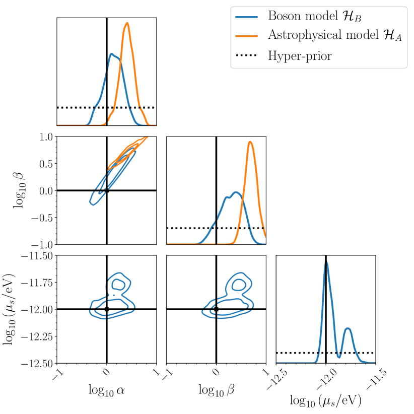
Figure 3: Corner plots of the $(\alpha,\beta,\mu_{s})$ hyperposterior assuming boson model $\mathcal{H}_{\mathrm{B}}$ (blue) and $\mathcal{H}_{\rm{A}}$ (orange) in $\mathrm{log}_{10}$ space. The contours are shown at 68% and 95% intervals. For this example, we average 50 sets of sources, each with 300 high SNR events drawing from the boson population at $\mu_{s}=10^{-12}$ eV and $(\alpha,\beta)=(1,1)$ (“flat spin”). The dashed and solid black lines are the hyperpriors and true values, respectively.

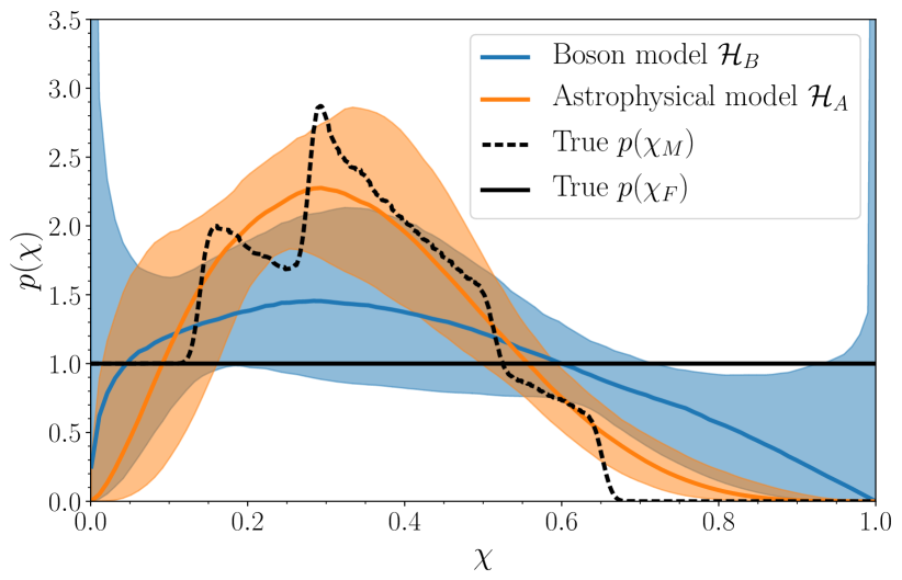
Figure 4: Hyperposterior of the spin distribution at formation $p(\chi_{F}|\alpha,\beta)$, inferred with the same set of simulations (flat spin and $\mu_{s}=10^{-12}$ eV) in Fig. 3. The blue (orange) solid line shows the median of the inferred $p(\chi_{F}|\alpha,\beta)$ assuming $\mathcal{H}_{\mathrm{B}}$ ($\mathcal{H}_{\rm{A}}$). The bands mark the 90% credible intervals. The dashed and solid black lines are the true spin distribution at merger and at formation, respectively, in this simulation with boson existence. The characteristic “zig-zag” structure in $p(\chi_{M})$ reflects the postsuperradiant spins of different superradiant modes.

VI Discussion

In this paper, we have illustrated the use of hierarchical Bayesian inference to simultaneously measure the BH spin distribution at formation and to search for ultralight bosons, by combining mass and spin measurements from a population of BBHs detected by GW observatories. Our method relies on the morphology of the expected exclusion region in the BH mass-spin plane, which depends on the properties of the boson mass, to search for and characterize the boson. Applying this method on a mock data set, we have shown that BBHs discovered by ground-based GW detectors can be used to rule out the existence of ultralight bosons in the mass range $[10^{-13},3\times 10^{-12}]$ eV. Our method is also capable to reveal the existence of a ultralight boson, and measure its mass, as we have explicitly shown with two example of boson masses, $\mu_{s}=10^{-13}$ eV and $10^{-12}$ eV. In order to investigate the impact of spin distribution at formation on the statistical power of our method, we have generated populations of simulated BBHs with either a uniform distribution or a linearly decreasing distribution of BH spins at formation. We found that in both cases combining $\lesssim 300$ high SNR events will be enough to rule out or confirm the existence of an ultralight boson within the mass range $[10^{-13},10^{-12}]$ eV.

While we only consider scalar bosons in this study, the method we developed is applicable to vector or tensor boson fields, which have much shorter instability and GW emission time scales [36, 38, 117]. Our analysis of simulated BBHs has made a few simplifying assumptions which make it conservative. First, we have assumed that all BBHs merge in 10 Myr, which is toward the lower limit of what is usually obtained in numerical simulations [97, 98, 99, 100, 101, 102, 103, 104, 105, 106, 107]. Since most of the BBHs in our parameters space of interest would have undergone superradiance within 10 Myr except for the very low mass systems $\sim 5M_{\odot}$, assuming longer merger times does not significantly improve the searching efficiency. Second, we have assumed that only sources with SNR$>30$ will contribute to this test, as their spins are easier to measure. In reality, while the component spins of weaker events are harder to measure, they will still contribute to the test.

In the analysis, we ignored the $\lesssim 10\%$ BH mass loss during superradiance. In order to assess the impact of this choice, we repeated the analysis with all BH mass posteriors shifted by $5\%$ toward the light side, hence mimicking the effect of mass loss. This translates to a systematic overestimation of $\sim 5\%$ boson mass, which is still within the statistical uncertainty, in our inference with $\mathcal{O}(100)$ high SNR sources. However, we expect this systematic error will dominate when the number of events grow to $\mathcal{O}(10^{4})$ in the era of next-generation detectors [118, 119, 120, 121, 122, 123, 124, 125].

The true distribution of spins at formation plays the most important role: the number of events needed to perform this test will be larger if the astrophysical distribution of spins at formation is such that small spins are preferred. Conversely, if many highly spinning BHs are formed, potentially with significant misalignments between spin and angular momenta (both of which make spins easier to measure), then fewer sources will be necessary. Given the measured BBH merger rate, ground-based interferometers will detect hundreds of BBHs per year at design sensitivity [126, 127, 128, 129, 130]. In this large-number observations regime, one will want to use more sophisticated models which also capture eventual correlations between the masses and spins of astrophysical BHs [72, 73, 75]. This may boost or suppress the statistical power of testing boson hypothesis in a different boson mass range, depending on the actual joint distribution of BH mass and spin at formation. We will leave investigating these systematics to future work.

Within the assumptions made in this study, it seems feasible to rule out the existence of ultralight bosons everywhere in the mass range of $[10^{-13},3\times 10^{-12}]$ eV with a few years of advanced detectors data. However, we note that fewer GW events would be required to rule out the bosons in a narrower boson mass range. Statistically proving the existence of these bosons will take longer, as more sources are required: the planned upgrades of LIGO and Virgo to their “plus” configurations might yield thousands of BBH events per year, which will make it more plausible to gather the evidence for the existence of ultralight bosons in the mass range of $[10^{-13},3\times 10^{-12}]$ eV [119, 121].

VII Acknowledgements

We thank the anonymous referees for their suggestions which significantly improved this paper. We also thank Emanuele Berti, Richard Brito, Will Farr, Carl Haster, Max Isi, and Kaze Wong for the valuable discussions and suggestions. K. K. Y. N. and S. V. acknowledge the support of the National Science Foundation (NSF) through the NSF Grant No. PHY-1836814. LIGO was constructed by the California Institute of Technology and Massachusetts Institute of Technology with funding from the National Science Foundation and operates under cooperative agreement PHY-1764464. The work of O. A. H. was supported by the Hong Kong Ph.D. Fellowship Scheme issued by the Research Grants Council of Hong Kong before resubmission and was supported by the research program of the Netherlands Organization for Scientific Research. The work of T. G. F. L. was partially supported by grants from the Research Grants Council of Hong Kong (Projects No. CUHK14306218, No. CUHK14310816, and No. CUHK24304317), Research Committee of the Chinese University of Hong Kong, and the Croucher Foundation in Hong Kong. This research made use of data, software, and/or web tools obtained from the Gravitational Wave Open Science Center [131], a service of LIGO Laboratory, the LIGO Scientific Collaboration, and the Virgo Collaboration. The authors are grateful for computational resources provided by the LIGO Lab and supported by the NSF Grants No. PHY-0757058 and No. PHY-0823459.

References

- Peccei and Quinn [1977a] R. Peccei and H. R. Quinn, CP Conservation in the Presence of Instantons, Phys. Rev. Lett. 38, 1440 (1977a).
- Weinberg [1978] S. Weinberg, A New Light Boson?, Phys. Rev. Lett. 40, 223 (1978).
- Wilczek [1978] F. Wilczek, Problem of Strong and Invariance in the Presence of Instantons, Phys. Rev. Lett. 40, 279 (1978).
- Dimopoulos and Giudice [1996] S. Dimopoulos and G. Giudice, Macroscopic forces from supersymmetry, Phys. Lett. B 379, 105 (1996), arXiv:hep-ph/9602350 .
- Goodsell et al. [2009] M. Goodsell, J. Jaeckel, J. Redondo, and A. Ringwald, Naturally Light Hidden Photons in LARGE Volume String Compactifications, JHEP 11, 027, arXiv:0909.0515 [hep-ph] .
- Arvanitaki et al. [2010] A. Arvanitaki, S. Dimopoulos, S. Dubovsky, N. Kaloper, and J. March-Russell, String Axiverse, Phys. Rev. D81, 123530 (2010), arXiv:0905.4720 [hep-th] .
- Preskill et al. [1983] J. Preskill, M. B. Wise, and F. Wilczek, Cosmology of the Invisible Axion, Phys. Lett. B 120, 127 (1983).
- Abbott and Sikivie [1983] L. Abbott and P. Sikivie, A Cosmological Bound on the Invisible Axion, Phys. Lett. B 120, 133 (1983).
- Dine and Fischler [1983] M. Dine and W. Fischler, The Not So Harmless Axion, Phys. Lett. B 120, 137 (1983).
- Turner and Wilczek [1991] M. S. Turner and F. Wilczek, Inflationary axion cosmology, Phys. Rev. Lett. 66, 5 (1991).
- Hu et al. [2000] W. Hu, R. Barkana, and A. Gruzinov, Cold and fuzzy dark matter, Phys. Rev. Lett. 85, 1158 (2000), arXiv:astro-ph/0003365 .
- Peccei and Quinn [1977b] R. Peccei and H. R. Quinn, Constraints Imposed by CP Conservation in the Presence of Instantons, Phys. Rev. D 16, 1791 (1977b).
- Peccei [2008] R. Peccei, The Strong CP problem and axions, Lect. Notes Phys. 741, 3 (2008), arXiv:hep-ph/0607268 .
- Bertone et al. [2005] G. Bertone, D. Hooper, and J. Silk, Particle dark matter: Evidence, candidates and constraints, Phys. Rept. 405, 279 (2005), arXiv:hep-ph/0404175 [hep-ph] .
- Hertzberg et al. [2008] M. P. Hertzberg, M. Tegmark, and F. Wilczek, Axion Cosmology and the Energy Scale of Inflation, Phys. Rev. D 78, 083507 (2008), arXiv:0807.1726 [astro-ph] .
- Jaeckel and Ringwald [2010] J. Jaeckel and A. Ringwald, The Low-Energy Frontier of Particle Physics, Ann. Rev. Nucl. Part. Sci. 60, 405 (2010), arXiv:1002.0329 [hep-ph] .
- Arvanitaki and Dubovsky [2011] A. Arvanitaki and S. Dubovsky, Exploring the String Axiverse with Precision Black Hole Physics, Phys. Rev. D83, 044026 (2011), arXiv:1004.3558 [hep-th] .
- Essig et al. [2013] R. Essig et al., Working Group Report: New Light Weakly Coupled Particles, in Proceedings, 2013 Community Summer Study on the Future of U.S. Particle Physics: Snowmass on the Mississippi (CSS2013): Minneapolis, MN, USA, July 29-August 6, 2013 (2013) arXiv:1311.0029 [hep-ph] .
- Marsh [2016] D. J. E. Marsh, Axion Cosmology, Phys. Rept. 643, 1 (2016), arXiv:1510.07633 [astro-ph.CO] .
- Hui et al. [2017] L. Hui, J. P. Ostriker, S. Tremaine, and E. Witten, Ultralight scalars as cosmological dark matter, Phys. Rev. D95, 043541 (2017), arXiv:1610.08297 [astro-ph.CO] .
- Arvanitaki et al. [2020] A. Arvanitaki, S. Dimopoulos, M. Galanis, L. Lehner, J. O. Thompson, and K. Van Tilburg, Large-misalignment mechanism for the formation of compact axion structures: Signatures from the QCD axion to fuzzy dark matter, Phys. Rev. D 101, 083014 (2020), arXiv:1909.11665 [astro-ph.CO] .
- Asztalos et al. [2010] S. Asztalos et al. (ADMX), A SQUID-based microwave cavity search for dark-matter axions, Phys. Rev. Lett. 104, 041301 (2010), arXiv:0910.5914 [astro-ph.CO] .
- Wagner et al. [2010] A. Wagner et al. (ADMX), A Search for Hidden Sector Photons with ADMX, Phys. Rev. Lett. 105, 171801 (2010), arXiv:1007.3766 [hep-ex] .
- Rybka et al. [2010] G. Rybka et al. (ADMX), A Search for Scalar Chameleons with ADMX, Phys. Rev. Lett. 105, 051801 (2010), arXiv:1004.5160 [astro-ph.CO] .
- Aune et al. [2011] S. Aune et al. (CAST), CAST search for sub-eV mass solar axions with 3He buffer gas, Phys. Rev. Lett. 107, 261302 (2011), arXiv:1106.3919 [hep-ex] .
- Pugnat et al. [2014] P. Pugnat et al. (OSQAR), Search for weakly interacting sub-eV particles with the OSQAR laser-based experiment: results and perspectives, Eur. Phys. J. C 74, 3027 (2014), arXiv:1306.0443 [hep-ex] .
- Arvanitaki et al. [2015a] A. Arvanitaki, J. Huang, and K. Van Tilburg, Searching for dilaton dark matter with atomic clocks, Phys. Rev. D91, 015015 (2015a), arXiv:1405.2925 [hep-ph] .
- Corasaniti et al. [2017] P. Corasaniti, S. Agarwal, D. Marsh, and S. Das, Constraints on dark matter scenarios from measurements of the galaxy luminosity function at high redshifts, Phys. Rev. D 95, 083512 (2017), arXiv:1611.05892 [astro-ph.CO] .
- Choi et al. [2017] J. Choi, H. Themann, M. Lee, B. Ko, and Y. Semertzidis, First axion dark matter search with toroidal geometry, Phys. Rev. D 96, 061102 (2017), arXiv:1704.07957 [hep-ex] .
- Akerib et al. [2017] D. Akerib et al. (LUX), First Searches for Axions and Axionlike Particles with the LUX Experiment, Phys. Rev. Lett. 118, 261301 (2017), arXiv:1704.02297 [astro-ph.CO] .
- Brubaker et al. [2017] B. Brubaker et al., First results from a microwave cavity axion search at 24 eV, Phys. Rev. Lett. 118, 061302 (2017), arXiv:1610.02580 [astro-ph.CO] .
- Kim et al. [2018] Y. J. Kim, P.-H. Chu, and I. Savukov, Experimental Constraint on an Exotic Spin- and Velocity-Dependent Interaction in the Sub-meV Range of Axion Mass with a Spin-Exchange Relaxation-Free Magnetometer, Phys. Rev. Lett. 121, 091802 (2018), arXiv:1702.02974 [physics.ins-det] .
- Garcon et al. [2017] A. Garcon et al., The Cosmic Axion Spin Precession Experiment (CASPEr): a dark-matter search with nuclear magnetic resonance, Quantum Science and Technology 10.1088/2058-9565/aa9861 (2017), arXiv:1707.05312 [physics.ins-det] .
- Arvanitaki et al. [2015b] A. Arvanitaki, M. Baryakhtar, and X. Huang, Discovering the QCD Axion with Black Holes and Gravitational Waves, Phys. Rev. D91, 084011 (2015b), arXiv:1411.2263 [hep-ph] .
- Arvanitaki et al. [2017] A. Arvanitaki, M. Baryakhtar, S. Dimopoulos, S. Dubovsky, and R. Lasenby, Black Hole Mergers and the QCD Axion at Advanced LIGO, Phys. Rev. D95, 043001 (2017), arXiv:1604.03958 [hep-ph] .
- Baryakhtar et al. [2017] M. Baryakhtar, R. Lasenby, and M. Teo, Black Hole Superradiance Signatures of Ultralight Vectors, Phys. Rev. D96, 035019 (2017), arXiv:1704.05081 [hep-ph] .
- Brito et al. [2017a] R. Brito, S. Ghosh, E. Barausse, E. Berti, V. Cardoso, I. Dvorkin, A. Klein, and P. Pani, Stochastic and resolvable gravitational waves from ultralight bosons, Phys. Rev. Lett. 119, 131101 (2017a), arXiv:1706.05097 [gr-qc] .
- Cardoso et al. [2018] V. Cardoso, O. J. C. Dias, G. S. Hartnett, M. Middleton, P. Pani, and J. E. Santos, Constraining the mass of dark photons and axion-like particles through black-hole superradiance, JCAP 1803 (03), 043, arXiv:1801.01420 [gr-qc] .
- D’Antonio et al. [2018] S. D’Antonio et al., Semicoherent analysis method to search for continuous gravitational waves emitted by ultralight boson clouds around spinning black holes, Phys. Rev. D 98, 103017 (2018), arXiv:1809.07202 [gr-qc] .
- Ghosh et al. [2019] S. Ghosh, E. Berti, R. Brito, and M. Richartz, Follow-up signals from superradiant instabilities of black hole merger remnants, Phys. Rev. D 99, 104030 (2019), arXiv:1812.01620 [gr-qc] .
- Tsukada et al. [2019] L. Tsukada, T. Callister, A. Matas, and P. Meyers, First search for a stochastic gravitational-wave background from ultralight bosons, Phys. Rev. D 99, 103015 (2019), arXiv:1812.09622 [astro-ph.HE] .
- Stott et al. [2017] M. J. Stott, D. J. E. Marsh, C. Pongkitivanichkul, L. C. Price, and B. S. Acharya, Spectrum of the axion dark sector, Phys. Rev. D 96, 083510 (2017), arXiv:1706.03236 [astro-ph.CO] .
- Hannuksela et al. [2019] O. A. Hannuksela, K. W. Wong, R. Brito, E. Berti, and T. G. Li, Probing the existence of ultralight bosons with a single gravitational-wave measurement, Nature Astron. 3, 447 (2019), arXiv:1804.09659 [astro-ph.HE] .
- Ouellet et al. [2019] J. L. Ouellet et al., First Results from ABRACADABRA-10 cm: A Search for Sub-eV Axion Dark Matter, Phys. Rev. Lett. 122, 121802 (2019), arXiv:1810.12257 [hep-ex] .
- Davoudiasl and Denton [2019] H. Davoudiasl and P. B. Denton, Ultralight Boson Dark Matter and Event Horizon Telescope Observations of M87*, Phys. Rev. Lett. 123, 021102 (2019), arXiv:1904.09242 [astro-ph.CO] .
- Fernandez et al. [2019] N. Fernandez, A. Ghalsasi, and S. Profumo, Superradiance and the Spins of Black Holes from LIGO and X-ray binaries, arXiv e-prints , arXiv:1911.07862 (2019), arXiv:1911.07862 [hep-ph] .
- Palomba et al. [2019] C. Palomba et al., Direct constraints on ultra-light boson mass from searches for continuous gravitational waves, Phys. Rev. Lett. 123, 171101 (2019), arXiv:1909.08854 [astro-ph.HE] .
- Ng et al. [2020a] K. K. Ng, M. Isi, C.-J. Haster, and S. Vitale, Multiband gravitational-wave searches for ultralight bosons, arXiv e-prints (2020a), arXiv:2007.12793 [gr-qc] .
- Abel et al. [2017] C. Abel et al., Search for Axionlike Dark Matter through Nuclear Spin Precession in Electric and Magnetic Fields, Phys. Rev. X7, 041034 (2017), arXiv:1708.06367 [hep-ph] .
- Grote and Stadnik [2019] H. Grote and Y. V. Stadnik, Novel signatures of dark matter in laser-interferometric gravitational-wave detectors, Phys. Rev. Research. 1, 033187 (2019), arXiv:1906.06193 [astro-ph.IM] .
- Dev et al. [2017] P. S. B. Dev, M. Lindner, and S. Ohmer, Gravitational waves as a new probe of Bose–Einstein condensate Dark Matter, Phys. Lett. B 773, 219 (2017), arXiv:1609.03939 [hep-ph] .
- Zhu et al. [2020] S. J. Zhu, M. Baryakhtar, M. A. Papa, D. Tsuna, N. Kawanaka, and H.-B. Eggenstein, Characterizing the continuous gravitational-wave signal from boson clouds around Galactic isolated black holes, Phys. Rev. D 102, 063020 (2020), arXiv:2003.03359 [gr-qc] .
- Ng et al. [2020b] K. K. Ng, S. Vitale, O. A. Hannuksela, and T. G. Li, Constraints on ultralight scalar bosons within black hole spin measurements from LIGO-Virgo’s GWTC-2, ArXiv e-print (2020b), arXiv:2011.06010 [gr-qc] .
- Zel’Dovich [1971] Y. B. Zel’Dovich, Generation of Waves by a Rotating Body, Soviet Journal of Experimental and Theoretical Physics Letters 14, 180 (1971).
- Zel’Dovich [1972] Y. B. Zel’Dovich, Amplification of Cylindrical Electromagnetic Waves Reflected from a Rotating Body, Soviet Journal of Experimental and Theoretical Physics 35, 1085 (1972).
- Press and Teukolsky [1972] W. H. Press and S. A. Teukolsky, Floating Orbits, Superradiant Scattering and the Black-hole Bomb, Nature 238, 211 (1972).
- Misner [1972] C. W. Misner, Interpretation of gravitational-wave observations, Phys. Rev. Lett. 28, 994 (1972).
- Dolan [2007] S. R. Dolan, Instability of the massive Klein-Gordon field on the Kerr spacetime, Phys. Rev. D76, 084001 (2007), arXiv:0705.2880 [gr-qc] .
- Brito et al. [2015a] R. Brito, V. Cardoso, and P. Pani, Black holes as particle detectors: evolution of superradiant instabilities, Class. Quant. Grav. 32, 134001 (2015a), arXiv:1411.0686 [gr-qc] .
- Brito et al. [2015b] R. Brito, V. Cardoso, and P. Pani, Superradiance, Lect. Notes Phys. 906, pp.1 (2015b), arXiv:1501.06570 [gr-qc] .
- Remillard and McClintock [2006] R. A. Remillard and J. E. McClintock, X-ray Properties of Black-Hole Binaries, Ann. Rev. Astron. Astrophys. 44, 49 (2006), arXiv:astro-ph/0606352 .
- Middleton [2016] M. Middleton, Black Hole Spin: Theory and Observation, in Astrophysics of Black Holes: From Fundamental Aspects to Latest Developments, Vol. 440, edited by C. Bambi (2016) p. 99.
- Corral-Santana et al. [2016] J. M. Corral-Santana, J. Casares, T. Munoz-Darias, F. E. Bauer, I. G. Martinez-Pais, and D. M. Russell, BlackCAT: A catalogue of stellar-mass black holes in X-ray transients, Astron. Astrophys. 587, A61 (2016), arXiv:1510.08869 [astro-ph.HE] .
- Aasi et al. [2015] J. Aasi et al. (LIGO Scientific), Advanced LIGO, Class. Quant. Grav. 32, 074001 (2015), arXiv:1411.4547 [gr-qc] .
- Acernese [2015] o. Acernese, F., Advanced Virgo: a second-generation interferometric gravitational wave detector, Classical and Quantum Gravity 32, 024001 (2015), arXiv:1408.3978 [gr-qc] .
- Abbott et al. [2019a] B. Abbott et al. (LIGO Scientific, Virgo), GWTC-1: A Gravitational-Wave Transient Catalog of Compact Binary Mergers Observed by LIGO and Virgo during the First and Second Observing Runs, Phys. Rev. X 9, 031040 (2019a), arXiv:1811.12907 [astro-ph.HE] .
- Abbott et al. [2020a] R. Abbott et al. (LIGO Scientific, Virgo), GWTC-2: Compact Binary Coalescences Observed by LIGO and Virgo During the First Half of the Third Observing Run, ArXiv e-print (2020a), arXiv:2010.14527 [gr-qc] .
- Vitale et al. [2014] S. Vitale, R. Lynch, J. Veitch, V. Raymond, and R. Sturani, Measuring the Spin of Black Holes in Binary Systems Using Gravitational Waves, Phys. Rev. Lett. 112, 251101 (2014), arXiv:1403.0129 [gr-qc] .
- Pürrer et al. [2016] M. Pürrer, M. Hannam, and F. Ohme, Can we measure individual black-hole spins from gravitational-wave observations?, Phys. Rev. D 93, 084042 (2016), arXiv:1512.04955 [gr-qc] .
- Vitale et al. [2017] S. Vitale, R. Lynch, V. Raymond, R. Sturani, J. Veitch, and P. Graff, Parameter estimation for heavy binary-black holes with networks of second-generation gravitational-wave detectors, Phys. Rev. D 95, 064053 (2017), arXiv:1611.01122 [gr-qc] .
- Fairhurst et al. [2020] S. Fairhurst, R. Green, C. Hoy, M. Hannam, and A. Muir, Two-harmonic approximation for gravitational waveforms from precessing binaries, Phys. Rev. D 102, 024055 (2020), arXiv:1908.05707 [gr-qc] .
- Belczynski et al. [2020] K. Belczynski et al., Evolutionary roads leading to low effective spins, high black hole masses, and O1/O2 rates for LIGO/Virgo binary black holes, Astron. Astrophys. 636, A104 (2020), arXiv:1706.07053 [astro-ph.HE] .
- Gerosa et al. [2018] D. Gerosa, E. Berti, R. O’Shaughnessy, K. Belczynski, M. Kesden, D. Wysocki, and W. Gladysz, Spin orientations of merging black holes formed from the evolution of stellar binaries, Phys. Rev. D 98, 084036 (2018), arXiv:1808.02491 [astro-ph.HE] .
- Postnov and Kuranov [2019] K. A. Postnov and A. G. Kuranov, Black hole spins in coalescing binary black holes, MNRAS 483, 3288 (2019), arXiv:1706.00369 [astro-ph.HE] .
- Bavera et al. [2020] S. S. Bavera, T. Fragos, Y. Qin, E. Zapartas, C. J. Neijssel, I. Mandel, A. Batta, S. M. Gaebel, C. Kimball, and S. Stevenson, The origin of spin in binary black holes: Predicting the distributions of the main observables of Advanced LIGO, Astron. Astrophys. 635, A97 (2020), arXiv:1906.12257 [astro-ph.HE] .
- Farr et al. [2017] W. M. Farr, S. Stevenson, M. C. Miller, I. Mandel, B. Farr, and A. Vecchio, Distinguishing spin-aligned and isotropic black hole populations with gravitational waves, Nature 548, 426 (2017).
- Roulet and Zaldarriaga [2019] J. Roulet and M. Zaldarriaga, Constraints on binary black hole populations from LIGO–Virgo detections, Mon. Not. Roy. Astron. Soc. 484, 4216 (2019), arXiv:1806.10610 [astro-ph.HE] .
- Thrane and Talbot [2019] E. Thrane and C. Talbot, An introduction to Bayesian inference in gravitational-wave astronomy: parameter estimation, model selection, and hierarchical models, Publ. Astron. Soc. Austral. 36, e010 (2019), arXiv:1809.02293 [astro-ph.IM] .
- Taylor and Gerosa [2018] S. R. Taylor and D. Gerosa, Mining gravitational-wave catalogs to understand binary stellar evolution: A new hierarchical Bayesian framework, Phys. Rev. D 98, 083017 (2018), arXiv:1806.08365 [astro-ph.HE] .
- Abbott et al. [2019b] B. Abbott et al. (LIGO Scientific, Virgo), Binary Black Hole Population Properties Inferred from the First and Second Observing Runs of Advanced LIGO and Advanced Virgo, Astrophys. J. Lett. 882, L24 (2019b), arXiv:1811.12940 [astro-ph.HE] .
- Gaebel et al. [2019] S. M. Gaebel, J. Veitch, T. Dent, and W. M. Farr, Digging the population of compact binary mergers out of the noise, MNRAS 484, 4008 (2019), arXiv:1809.03815 [astro-ph.IM] .
- Mandel et al. [2019] I. Mandel, W. M. Farr, and J. R. Gair, Extracting distribution parameters from multiple uncertain observations with selection biases, MNRAS 486, 1086 (2019), arXiv:1809.02063 [physics.data-an] .
- Vitale [2020] S. Vitale, One, No One, and One Hundred Thousand – Inferring the properties of a population in presence of selection effects, arXiv e-prints (2020), arXiv:2007.05579 [astro-ph.IM] .
- Roulet et al. [2020] J. Roulet, T. Venumadhav, B. Zackay, L. Dai, and M. Zaldarriaga, Binary Black Hole Mergers from LIGO/Virgo O1 and O2: Population Inference Combining Confident and Marginal Events, arXiv e-prints (2020), arXiv:2008.07014 [astro-ph.HE] .
- Detweiler [1980] S. L. Detweiler, Klein-Gordon equation and rotating black holes, Phys. Rev. D22, 2323 (1980).
- Ficarra et al. [2019] G. Ficarra, P. Pani, and H. Witek, Impact of multiple modes on the black-hole superradiant instability, Phys. Rev. D 99, 104019 (2019), arXiv:1812.02758 [gr-qc] .
- Baryakhtar et al. [2020] M. Baryakhtar, M. Galanis, R. Lasenby, and O. Simon, Black hole superradiance of self-interacting scalar fields, ArXiv e-print (2020), arXiv:2011.11646 [hep-ph] .
- Brito et al. [2017b] R. Brito, S. Ghosh, E. Barausse, E. Berti, V. Cardoso, I. Dvorkin, A. Klein, and P. Pani, Gravitational wave searches for ultralight bosons with LIGO and LISA, Phys. Rev. D96, 064050 (2017b), arXiv:1706.06311 [gr-qc] .
- Baumann et al. [2019] D. Baumann, H. S. Chia, and R. A. Porto, Probing ultralight bosons with binary black holes, Physical Review D 99, 044001 (2019).
- Berti et al. [2019] E. Berti, R. Brito, C. F. Macedo, G. Raposo, and J. L. Rosa, Ultralight boson cloud depletion in binary systems, Physical Review D 99, 104039 (2019).
- Baumann et al. [2020] D. Baumann, H. S. Chia, R. A. Porto, and J. Stout, Gravitational Collider Physics, Phys. Rev. D 101, 083019 (2020), arXiv:1912.04932 [gr-qc] .
- Zhang and Yang [2019a] J. Zhang and H. Yang, Gravitational floating orbits around hairy black holes, Phys. Rev. D 99, 064018 (2019a), arXiv:1808.02905 [gr-qc] .
- Zhang and Yang [2019b] J. Zhang and H. Yang, Dynamic Signatures of Black Hole Binaries with Superradiant Clouds, arXiv e-prints , arXiv:1907.13582 (2019b), arXiv:1907.13582 [gr-qc] .
- Wysocki et al. [2018] D. Wysocki, J. Lange, and R. O’Shaughnessy, Reconstructing phenomenological distributions of compact binaries via gravitational wave observations, arXiv e-prints , arXiv:1805.06442 (2018), arXiv:1805.06442 [gr-qc] .
- Abbott et al. [2016] B. P. Abbott, R. Abbott, T. D. Abbott, M. R. Abernathy, F. Acernese, K. Ackley, C. Adams, T. Adams, P. Addesso, and R. X. Adhikari, Properties of the Binary Black Hole Merger GW150914, Phys. Rev. Lett. 116, 241102 (2016), arXiv:1602.03840 [gr-qc] .
- Salpeter [1955] E. E. Salpeter, The Luminosity function and stellar evolution, Astrophys. J. 121, 161 (1955).
- Portegies Zwart and McMillan [2000] S. F. Portegies Zwart and S. L. W. McMillan, Black Hole Mergers in the Universe, Astrophysical Journal Letters 528, L17 (2000), astro-ph/9910061 .
- Miller and Lauburg [2009] M. C. Miller and V. M. Lauburg, Mergers of Stellar-Mass Black Holes in Nuclear Star Clusters, ApJ 692, 917 (2009), arXiv:0804.2783 .
- O’Leary et al. [2009] R. M. O’Leary, B. Kocsis, and A. Loeb, Gravitational waves from scattering of stellar-mass black holes in galactic nuclei, MNRAS 395, 2127 (2009), arXiv:0807.2638 .
- Downing et al. [2011] J. M. B. Downing, M. J. Benacquista, M. Giersz, and R. Spurzem, Compact binaries in star clusters - II. Escapers and detection rates, MNRAS 416, 133 (2011), arXiv:1008.5060 .
- Kocsis and Levin [2012] B. Kocsis and J. Levin, Repeated bursts from relativistic scattering of compact objects in galactic nuclei, Phys. Rev. D 85, 123005 (2012), arXiv:1109.4170 [astro-ph.CO] .
- Tsang [2013] D. Tsang, Shattering Flares during Close Encounters of Neutron Stars, ApJ 777, 103 (2013), arXiv:1307.3554 [astro-ph.HE] .
- Ziosi et al. [2014] B. M. Ziosi, M. Mapelli, M. Branchesi, and G. Tormen, Dynamics of stellar black holes in young star clusters with different metallicities - II. Black hole-black hole binaries, MNRAS 441, 3703 (2014), arXiv:1404.7147 .
- Rodriguez et al. [2015] C. L. Rodriguez, M. Morscher, B. Pattabiraman, S. Chatterjee, C.-J. Haster, and F. A. Rasio, Binary Black Hole Mergers from Globular Clusters: Implications for Advanced LIGO, Physical Review Letters 115, 051101 (2015), arXiv:1505.00792 [astro-ph.HE] .
- Rodriguez et al. [2016] C. L. Rodriguez, M. Morscher, B. Pattabiraman, S. Chatterjee, C.-J. Haster, and F. A. Rasio, Erratum: Binary Black Hole Mergers from Globular Clusters: Implications for Advanced LIGO [Phys. Rev. Lett. 115, 051101 (2015)], Physical Review Letters 116, 029901 (2016).
- Morscher et al. [2015] M. Morscher, B. Pattabiraman, C. Rodriguez, F. A. Rasio, and S. Umbreit, The Dynamical Evolution of Stellar Black Holes in Globular Clusters, ApJ 800, 9 (2015), arXiv:1409.0866 .
- Dominik et al. [2013] M. Dominik, K. Belczynski, C. Fryer, D. E. Holz, E. Berti, T. Bulik, I. Mandel, and R. O’Shaughnessy, Double compact objects. ii. cosmological merger rates, The Astrophysical Journal 779, 72 (2013).
- Ng et al. [2018] K. K. Y. Ng, S. Vitale, A. Zimmerman, K. Chatziioannou, D. Gerosa, and C.-J. Haster, Gravitational-wave astrophysics with effective-spin measurements: Asymmetries and selection biases, Phys. Rev. D 98, 083007 (2018), arXiv:1805.03046 [gr-qc] .
- Barsotti et al. [2018] L. Barsotti, S. Gras, M. Evans, and P. Fritschel, Updated Advanced LIGO sensitivity design curve, https://dcc.ligo.org/T1800044-v5/public (2018), Technical Report LIGO-T1800044-v5.
- Abbott et al. [2018] B. P. Abbott et al., Prospects for observing and localizing gravitational-wave transients with Advanced LIGO, Advanced Virgo and KAGRA, Living Reviews in Relativity 21, 3 (2018), arXiv:1304.0670 [gr-qc] .
- Veitch et al. [2015] J. Veitch et al., Parameter estimation for compact binaries with ground-based gravitational-wave observations using the LALInference software library, Phys. Rev. D 91, 042003 (2015), arXiv:1409.7215 [gr-qc] .
- LIGO Scientific Collaboration [2018] LIGO Scientific Collaboration, LIGO Algorithm Library - LALSuite, free software (GPL) (2018), https://git.ligo.org/lscsoft/lalsuite.
- Smith et al. [2016] R. Smith, S. E. Field, K. Blackburn, C.-J. Haster, M. Purrer, V. Raymond, and P. Schmidt, Fast and accurate inference on gravitational waves from precessing compact binaries, Physical Review D 94, 044031 (2016).
- Schutz [2011] B. F. Schutz, Networks of gravitational wave detectors and three figures of merit, Class. Quant. Grav. 28, 125023 (2011), arXiv:1102.5421 [astro-ph.IM] .
- Ly et al. [2016] A. Ly, J. Verhagen, and E.-J. Wagenmakers, Harold jeffreys’s default bayes factor hypothesis tests: Explanation, extension, and application in psychology, Journal of Mathematical Psychology 72, 19 (2016).
- Abbott et al. [2020b] R. Abbott et al. (LIGO Scientific, Virgo), Population Properties of Compact Objects from the Second LIGO-Virgo Gravitational-Wave Transient Catalog, Arxiv e-print (2020b), arXiv:2010.14533 [astro-ph.HE] .
- Brito et al. [2020] R. Brito, S. Grillo, and P. Pani, Black hole superradiant instability from ultralight spin-2 fields, Phys. Rev. Lett. 124, 211101 (2020), arXiv:2002.04055 [gr-qc] .
- Punturo et al. [2010] M. Punturo et al., The Einstein Telescope: A third-generation gravitational wave observatory, Class. Quant. Grav. 27, 194002 (2010).
- LIGO Scientific Collaboration [2018] LIGO Scientific Collaboration, Instrument Science White Paper 2018, https://dcc.ligo.org/T1800133/public (2018), Technical Report LIGO-T1800133.
- Vitale et al. [2019] S. Vitale, W. M. Farr, K. Ng, and C. L. Rodriguez, Measuring the star formation rate with gravitational waves from binary black holes, Astrophys. J. Lett. 886, L1 (2019), arXiv:1808.00901 [astro-ph.HE] .
- Shoemaker [2019] D. Shoemaker (LIGO Scientific), Gravitational wave astronomy with LIGO and similar detectors in the next decade, arXiv e-prints (2019), arXiv:1904.03187 [gr-qc] .
- Maggiore et al. [2020] M. Maggiore et al., Science Case for the Einstein Telescope, JCAP 03, 050, arXiv:1912.02622 [astro-ph.CO] .
- Reitze et al. [2019] D. Reitze et al., Cosmic Explorer: The U.S. Contribution to Gravitational-Wave Astronomy beyond LIGO, Bull. Am. Astron. Soc. 51, 035 (2019), arXiv:1907.04833 [astro-ph.IM] .
- Adhikari et al. [2019] R. X. Adhikari et al., Astrophysical science metrics for next-generation gravitational-wave detectors, Class. Quant. Grav. 36, 245010 (2019), arXiv:1905.02842 [astro-ph.HE] .
- Hall and Evans [2019] E. D. Hall and M. Evans, Metrics for next-generation gravitational-wave detectors, Class. Quant. Grav. 36, 225002 (2019), arXiv:1902.09485 [astro-ph.IM] .
- Dominik et al. [2015] M. Dominik, E. Berti, R. O’Shaughnessy, I. Mandel, K. Belczynski, C. Fryer, D. E. Holz, T. Bulik, and F. Pannarale, Double Compact Objects III: Gravitational Wave Detection Rates, Astrophys. J. 806, 263 (2015), arXiv:1405.7016 [astro-ph.HE] .
- Ng et al. [2018] K. K. Ng, K. W. Wong, T. Broadhurst, and T. G. Li, Precise LIGO Lensing Rate Predictions for Binary Black Holes, Phys. Rev. D 97, 023012 (2018), arXiv:1703.06319 [astro-ph.CO] .
- Oguri [2018] M. Oguri, Effect of gravitational lensing on the distribution of gravitational waves from distant binary black hole mergers, Mon. Not. Roy. Astron. Soc. 480, 3842 (2018), arXiv:1807.02584 [astro-ph.CO] .
- Baibhav et al. [2019] V. Baibhav, E. Berti, D. Gerosa, M. Mapelli, N. Giacobbo, Y. Bouffanais, and U. N. Di Carlo, Gravitational-wave detection rates for compact binaries formed in isolation: LIGO/Virgo O3 and beyond, Phys. Rev. D100, 064060 (2019), arXiv:1906.04197 [gr-qc] .
- Abbott et al. [2018] B. P. Abbott et al. (KAGRA, LIGO Scientific, VIRGO), Prospects for Observing and Localizing Gravitational-Wave Transients with Advanced LIGO, Advanced Virgo and KAGRA, Living Rev. Rel. 21, 3 (2018), arXiv:1304.0670 [gr-qc] .
- Abbott et al. [2021] R. Abbott et al., Open data from the first and second observing runs of advanced ligo and advanced virgo, SoftwareX 13, 100658 (2021).