Knowledge Consistency between Neural Networks and Beyond
Abstract
This paper aims to analyze knowledge consistency between pre-trained deep neural networks. We propose a generic definition for knowledge consistency between neural networks at different fuzziness levels. A task-agnostic method is designed to disentangle feature components, which represent the consistent knowledge, from raw intermediate-layer features of each neural network. As a generic tool, our method can be broadly used for different applications. In preliminary experiments, we have used knowledge consistency as a tool to diagnose representations of neural networks. Knowledge consistency provides new insights to explain the success of existing deep-learning techniques, such as knowledge distillation and network compression. More crucially, knowledge consistency can also be used to refine pre-trained networks and boost performance.
1 Introduction
Deep neural networks (DNNs) have shown promise in many tasks of artificial intelligence. However, there is still lack of mathematical tools to diagnose representations in intermediate layers of a DNN, e.g. discovering flaws in representations or identifying reliable and unreliable features. Traditional evaluation of DNNs based on the testing accuracy cannot insightfully examine the correctness of representations of a DNN due to leaked data or shifted datasets (Ribeiro et al., 2016).
Thus, in this paper, we propose a method to diagnose representations of intermediate layers of a DNN from the perspective of knowledge consistency. I.e. given two DNNs pre-trained for the same task, no matter whether the DNNs have the same or different architectures, we aim to examine whether intermediate layers of the two DNNs encode similar visual concepts.
Here, we define the knowledge of an intermediate layer of the DNN as the set of visual concepts that are encoded by features of an intermediate layer. This research focuses on the consistency of “knowledge” between two DNNs, instead of comparing the similarity of “features.” In comparison, the feature is referred to as the explicit output of a layer. For example, two DNNs extract totally different features, but these features may be computed using similar sets of visual concepts, i.e. encoding consistent knowledge (a toy example of knowledge consistency is shown in the footnote111As a toy example, we show how to revise a pre-trained DNN to generate different features but represent consistent knowledge. The revised DNN shuffles feature elements in a layer and shuffles the feature back in the next convolutional layer , where ; is a permutation matrix. The knowledge encoded in the shuffled feature is consistent with the knowledge in the original feature.).
Given the same training data, DNNs with different starting conditions usually converge to different knowledge representations, which sometimes leads to the over-fitting problem (Bengio et al., 2014). However, ideally, well learned DNNs with high robustness usually comprehensively encode various types of discriminative features and keep a good balance between the completeness and the discrimination power of features (Wolchover, 2017). Thus, the well learned DNNs are supposed to converge to similar knowledge representations.

In general, we can understand knowledge consistency as follows. Let and denote two DNNs learned for the same task. and denote two intermediate-layer features of and , respectively. Features and can be decomposed as and , where neural activations in feature components and are triggered by same image regions, thereby representing consistent knowledge. Accordingly, feature components and are termed consistent features between and . Then, feature components and are independent with each other, and they are termed inconsistent features. We assume that consistent components can reconstruct each other, i.e. can be reconstructed from ; vice versa.
In terms of applications, knowledge consistency between DNNs can be used to diagnose feature reliability of DNNs. Usually, consistent components represent common and reliable knowledge. Whereas, inconsistent components mainly represent unreliable knowledge or noises.
Therefore, in this paper, we propose a generic definition for knowledge consistency between two pre-trained DNNs, and we develop a method to disentangle consistent feature components from features of intermediate layers in the DNNs. Our method is task-agnostic, i.e. (1) our method does not require any annotations w.r.t. the task for evaluation; (2) our method can be broadly applied to different DNNs as a supplement evaluation of DNNs besides the testing accuracy. Experimental results supported our assumption, i.e. the disentangled consistent feature components are usually more reliable for the task. Thus, our method of disentangling consistent features can be used to boost performance.
Furthermore, to enable a solid research on knowledge consistency, we consider the following issues.
Fuzzy consistency at different levels (orders): As shown in Fig. 1, the knowledge consistency between DNNs needs to be defined at different fuzziness levels, because there is no strict knowledge consistency between two DNNs. The level of fuzziness in knowledge consistency measures the difficulty of transforming features of a DNN to features of another DNN. A low-level fuzziness indicates that a DNN’s feature can directly reconstruct another DNN’s feature without complex transformations.
Disentanglement & quantification: We need to disentangle and quantify feature components, which correspond to the consistent knowledge at different fuzziness levels, away from the chaotic feature. Similarly, we also disentangle and quantify feature components that are inconsistent.
There does not exist a standard method to quantify the fuzziness of knowledge consistency (i.e. the difficulty of feature transformation). For simplification, we use non-linear transformations during feature reconstruction to approximate the fuzziness. To this end, we propose a model for feature reconstruction. The subscript indicates that contains a total of cascaded non-linear activation layers. represents components, which are disentangled from the feature of the DNN and can be reconstructed by the DNN ’s feature . Then, we consider to represent consistent knowledge w.r.t. the DNN at the -th fuzziness level (or the -th order). is also termed the -order consistent feature of w.r.t. .
In this way, the most strict consistency is the 0-order consistency, i.e. can be reconstructed from via a linear transformation. In comparison, some neural activations in the 1-order consistent feature are not directly represented by and need to be predicted via a non-linear transformation. The smaller indicates the less prediction involved in the reconstruction and the stricter consistency. Note that the number of non-linear operations is just a rough approximation of the difficulty of prediction, since there are no standard methods to quantify prediction difficulties.
More crucially, we implement the model as a neural network, where is set as the number of non-linear layers in . As shown in Fig. 2, is designed to disentangle and quantify consistent feature components of different orders between DNNs. Our method can be applied to different types of DNNs and explain the essence of various deep-learning techniques.
1. Our method provides a new perspective for explaining the effectiveness of knowledge distillation. I.e. we explore the essential reason why the born-again network (Furlanello et al., 2018) exhibits superior performance.
2. Our method gives insightful analysis of network compression.
3. Our method can be used to diagnose and refine knowledge representations of pre-trained DNNs and boost the performance without any additional annotations for supervision.
Contributions of this study can be summarized as follows. (1) In this study, we focus on a new problem, i.e. the knowledge consistency between DNNs. (2) We define the knowledge consistency and propose a task-agnostic method to disentangle and quantify consistent features of different orders. (3) Our method can be considered as a mathematical tool to analyze feature reliability of different DNNs. (4) Our method provides a new perspective on explaining existing deep-learning techniques, such as knowledge distillation and network compression.
2 Related work
In spite of the significant discrimination power of DNNs, black-box representations of DNNs have been considered an Achilles’ heel for decades. In this section, we will limit our discussion to the literature of explaining or analyzing knowledge representations of DNNs. In general, previous studies can be roughly classified into the following three types.
Explaining DNNs visually or semantically: Visualization of DNNs is the most direct way of explaining knowledge hidden inside a DNN, which include gradient-based visualization (Zeiler & Fergus, 2014; Mahendran & Vedaldi, 2015) and inversion-based visualization (Dosovitskiy & Brox, 2016). (Zhou et al., 2015) developed a method to compute the actual image-resolution receptive field of neural activations in a feature map of a convolutional neural network (CNN), which is smaller than the theoretical receptive field based on the filter size. Based on the receptive field, six types of semantics were defined to explain intermediate-layer features of CNNs, including objects, parts, scenes, textures, materials, and colors (Bau et al., 2017; Zhou et al., 2018).
Beyond visualization, some methods diagnose a pre-trained CNN to obtain insight understanding of CNN representations. Fong and Vedaldi (Fong & Vedaldi, 2018) analyzed how multiple filters jointly represented a specific semantic concept. (Selvaraju et al., 2017), (Fong & Vedaldi, 2017), and (Kindermans et al., 2018) estimated image regions that directly contributed the network output. The LIME (Ribeiro et al., 2016) and SHAP (Lundberg & Lee, 2017) assumed a linear relationship between the input and output of a DNN to extract important input units. (Zhang et al., 2019) proposed a number of metrics to evaluate the objectiveness of explanation results of different explanation methods, even when people could not get ground-truth explanations for the DNN.
Unlike previous studies visualizing visual appearance encoded in a DNN or extracting important pixels, our method disentangles and quantifies the consistent components of features between two DNNs. Consistent feature components of different orders can be explicitly visualized.
Learning explainable deep models: Compared to the post-hoc explanations of DNNs, some studies directly learn more meaningful CNN representations. Previous studies extracted scene semantics (Zhou et al., 2015) and mined objects (Simon & Rodner, 2015) from intermediate layers. In the capsule net (Sabour et al., 2017), each output dimension of a capsule usually encoded a specific meaning. (Zhang et al., 2018b) proposed to learn CNNs with disentangled intermediate-layer representations. The infoGAN (Chen et al., 2016) and -VAE (Higgins et al., 2017) learned interpretable input codes for generative models.
Mathematical evaluation of the representation capacity: Formulating and evaluating the representation capacity of DNNs is another emerging direction. (Novak et al., 2018) proposed generic metrics for the sensitivity of network outputs with respect to parameters of neural networks. (Zhang et al., 2017) discussed the relationship between the parameter number and the generalization capacity of deep neural networks. (Arpit et al., 2017) discussed the representation capacity of neural networks, considering real training data and noises. (Yosinski et al., 2014) evaluated the transferability of filters in intermediate layers. Network-attack methods (Koh & Liang, 2017; Szegedy et al., 2014; Koh & Liang, 2017) can also be used to evaluate representation robustness by computing adversarial samples. (Lakkaraju et al., 2017) discovered knowledge blind spots of the knowledge encoded by a DNN via human-computer interaction. (Zhang et al., 2018a) discovered potential, biased representations of a CNN due to the dataset bias. (Deutsch, 2018) learned the manifold of network parameters to diagnose DNNs. (Huang et al., 2019) quantified the representation utility of different layerwise network architectures in the scenario of 3D point cloud processing. Recently, the stiffness (Fort et al., 2019) was proposed to evaluate the generalization of DNNs.
The information-bottleneck theory (Wolchover, 2017; Schwartz-Ziv & Tishby, 2017) provides a generic metric to quantify the information contained in DNNs. The information-bottleneck theory can be extended to evaluate the representation capacity of DNNs (Xu & Raginsky, 2017; Cheng et al., 2018). (Achille & Soatto, 2018) further used the information-bottleneck theory to improve feature representations of a DNN. (Guan et al., 2019; Ma et al., 2019) quantified the word-wise/pixel-wise information discarding during the layerwise feature propagation of a DNN, and used the information discarding as a tool to diagnose feature representations.
The analysis of representation similarity between DNNs is most highly related to our research, which has been investigated in recent years (Montavon et al., 2011). Most previous studies (Wang et al., 2018; Kornblith et al., 2019; Raghu et al., 2017; Morcos et al., 2018) compared representations via linear transformations, which can be considered as 0-order knowledge consistency. In comparison, we focus on high-order knowledge consistency. More crucially, our method can be used to refine network features and explain the success of existing deep-learning techniques.
3 Algorithm
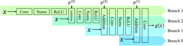
In this section, we will introduce the network architecture to disentangle feature components of consistent knowledge at a certain fuzziness level, when we use the intermediate-layer feature of a DNN to reconstruct intermediate-layer feature of another DNN222Re-scaling the magnitude of all neural activations does not affect the knowledge encoded in the DNN. Therefore, we normalize and to zero mean and unit variance to remove the magnitude effect.. As shown in Fig. 2, the network with parameters has a recursive architecture with blocks. The function of the -th block is given as follows.
| (1) |
The output feature is computed using both the raw input and the feature of the higher order . denotes a linear operation without a bias term. The last block is given as . This linear operation can be implemented as either a layer in an MLP or a convolutional layer in a CNN. is referred to a diagonal matrix for element-wise variance of , where the variance of the -th element of through various input images. is used to normalize the magnitude of neural activations. Because of the normalization, the scalar value roughly controls the activation magnitude of w.r.t. . corresponds to final output of the network.
In this way, the entire network can be separated into branches (see Fig. 2), where the -th branch () contains a total of non-linear layers. Note that the -order consistent knowledge can also be represented by the network with -th branch, if .
In order to disentangle consistent features of different orders, the -th branch is supposed to exclusively encode the -order consistent features without representing lower-order consistent features. Thus, we propose the following loss to guide the learning process.
| (2) |
where and denote intermediate-layer features of two pre-trained DNNs. The second term in this loss penalizes neural activations from high-order branches, thereby forcing as much low-order consistent knowledge as possible to be represented by low-order branches.
Furthermore, based on branches of the network, we can disentangle features of into additive components.
| (3) |
where indicates feature components that cannot be represented by . denotes feature components that are exclusively represented by the -order branch.
Based on Equation (1), the signal-processing procedure for the -th feature component can be represented as (see Fig. 2). Therefore, we can disentangle from Equation (1) all linear and non-linear operations along the entire -th branch as follows, and in this way, can be considered as the -order consistent feature component.
| (4) |
where is a diagonal matrix. Each diagonal element represents the binary information-passing state of through an ReLU layer (). Each element is given as , where . Note that , but . Thus, we record such information-passing states to decompose feature components.
4 Comparative studies
As a generic tool, knowledge consistency based on can be used for different applications. In order to demonstrate utilities of knowledge consistency, we designed various comparative studies, including (1) diagnosing and debugging pre-trained DNNs, (2) evaluating the instability of learning DNNs, (3) feature refinement of DNNs, (4) analyzing information discarding during the compression of DNNs, and (5) explaining effects of knowledge distillation in knowledge representations.
A total of five typical DNNs for image classification were used, i.e. the AlexNet (Krizhevsky et al., 2012), the VGG-16 (Simonyan & Zisserman, 2015), and the ResNet-18, ResNet-34, ResNet-50 (He et al., 2016). These DNNs were learned using three benchmark datasets, which included the CUB200-2011 dataset (Wah et al., 2011), the Stanford Dogs dataset (Khosla et al., 2011), and the Pascal VOC 2012 dataset (Everingham et al., 2015). Note that both training images and testing images were cropped using bounding boxes of objects. We set for all experiments, except for feature reconstruction of AlexNet (we set for AlexNet features). It was because the shallow model of the AlexNet usually had significant noisy features, which caused considerable inconsistent components.
4.1 Network diagnosis based on knowledge consistency
The most direct application of knowledge consistency is to use a strong (well learned) DNN to diagnose representation flaws hidden in a weak DNN. This is of special values in real applications, e.g. shallow (usually weak) DNNs are more suitable to be adopted to mobile devices than deep DNNs. Let two DNNs be trained for the same task, and one DNN significantly outperforms the other DNN. We assume that the strong DNN has encoded ideal knowledge representations of the target task. The weak DNN may have the following two types of representation flaws.
Unreliable features in the weak DNN are defined as feature components, which cannot be reconstructed by features of the strong DNN. (see Appendix B for detailed discussions).
Blind spots of the weak DNN are defined as feature components in the strong DNN, which are inconsistent with features of the weak DNN. These feature components usually reflect blind spots of the knowledge of the weak DNN (see Appendix B for detailed discussions).
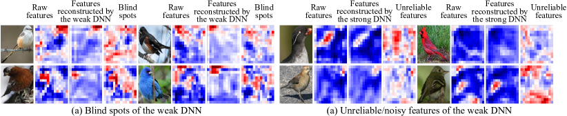
For implementation, we trained DNNs for fine-grained classification using the CUB200-2011 dataset (Wah et al., 2011) (without data augmentation). We considered the AlexNet (Krizhevsky et al., 2012) as the weak DNN (56.97% top-1 accuracy), and took the ResNet-34 (He et al., 2016) as the strong DNN (73.09% top-1 accuracy).
Please see Fig. 3. We diagnosed the output feature of the last convolutional layer in the AlexNet, which is termed . Accordingly, we selected the last feature map of the ResNet-34 (denoted by ) for the computation of knowledge consistency, because and had similar map sizes. We disentangled and visualized unreliable components from (i.e. inconsistent components in ). We also visualized components disentangled from (i.e. inconsistent components in ), which corresponded to blind spots of the weak DNN’s knowledge.
Furthermore, we conducted two experiments to further verify the claim of blind spots and unreliable features in a DNN. The first experiment aimed to verify blind spots. The basic idea of this experiment was to examine the increase of the classification accuracy, when we added information of blind spots to the raw feature. We followed above experimental settings, which used the intermediate-layer feature of the AlexNet (with 56.97% top-1 accuracy) to reconstruct the intermediate-layer feature of Resnet-34 (with 73.09% top-1 accuracy). Then, inconsistent feature components were termed blind spots. In this way, we added feature components of blind spots back to the AlexNet’s feature (adding these features back to ), and then learned a classifier upon the new feature. To enable a fair comparison, the classifier had the same architecture as the AlexNet’s modules above , and during the learning process, we fixed parameters in DNN A and to avoid the revision of such parameters affecting the performance. We found that compared to the raw feature of the AlexNet, the new feature boosted the classification accuracy by 16.1%.
The second experiment was conducted to verify unreliable features. The basic idea of this experiment was to examine the increase of the classification accuracy, when we removed information of unreliable features from the raw feature. We designed two classifiers, which had the same architecture as the AlexNet’s modules above . We fed the raw feature to the first classifier. Then, we removed unreliable feature components from (i.e. obtaining ), and fed the revised feature to the second classifier. We learned these two classifiers, and classifiers with and without unreliable features exhibited classification accuracy of 60.3% and 65.6%, respectively.
Therefore, above two experiments successfully demonstrated that both the insertion of blind spots and the removal of unreliable features boosted the classification accuracy.
4.2 Stability of learning
The stability of learning DNNs is of considerable values in deep learning, i.e. examining whether or not all DNNs represent the same knowledge, when people repeatedly learn multiple DNNs for the same task. High knowledge consistency between DNNs usually indicates high learning stability.
More specifically, we trained two DNNs with the same architecture for the same task. Then, we disentangled inconsistent feature components and from their features and of a specific layer, respectively. Accordingly, and corresponded to consistent feature components in and , respectively, whose knowledge was shared by two networks. The inconsistent feature was quantified by the variance of feature element through different units of and through different input images , where denotes the -th element of given the image . We can use to measure the instability of learning DNNs and .
In experiments, we evaluated the instability of learning the AlexNet (Krizhevsky et al., 2012), the VGG-16 (Simonyan & Zisserman, 2015), and the ResNet-34 (He et al., 2016). We considered the following cases.
Case 1, learning DNNs from different initializations using the same training data: For each network architecture, we trained multiple networks using the CUB200-2011 dataset (Wah et al., 2011). The instability of learning DNNs was reported as the average of instability over all pairs of neural networks.
Case 2, learning DNNs using different sets of training data: We randomly divided all training samples in the CUB200-2011 dataset (Wah et al., 2011) into two subsets, each containing 50% samples. For each network architecture, we trained two DNNs for fine-grained classification (without pre-training). The instability of learning DNNs was reported as .
Table 1 compares the instability of learning different DNNs. Table 2 reports the variance of consistent components of different orders. We found that the learning of shallow layers in DNNs was usually more stable than the learning of deep layers. The reason may be as follows. A DNN with more layers usually can represent more complex visual patterns, thereby needing more training samples. Without a huge training set (e.g. the ImageNet dataset (Krizhevsky et al., 2012)), a deep network may be more likely to suffer from the over-fitting problem, which causes high variances in Table 1, i.e. DNNs with different initial parameters may learn different knowledge representations.
| Learning DNNs from different initializations | ||||
|---|---|---|---|---|
| conv4 @ AlexNet | conv5 @ AlexNet | conv4-3 @ VGG-16 | conv5-3 @ VGG-16 | last conv @ ResNet-34 |
| 0.086 | 0.116 | 0.124 | 0.196 | 0.776 |
| Learning DNNs using different training data | ||||
| conv4 @ AlexNet | conv5 @ AlexNet | conv4-3 @ VGG-16 | conv5-3 @ VGG-16 | last conv @ ResNet-34 |
| 0.089 | 0.155 | 0.121 | 0.198 | 0.275 |
| conv4 @ AlexNet | conv5 @ AlexNet | conv4-3 @ VGG-16 | conv5-3 @ VGG-16 | last conv @ ResNet-34 | |
|---|---|---|---|---|---|
| 105.80 | 424.67 | 1.06 | 0.88 | 0.66 | |
| 10.51 | 73.73 | 0.07 | 0.03 | 0.10 | |
| 1.92 | 43.69 | 0.02 | 0.004 | 0.03 | |
| 11.14 | 71.37 | 0.16 | 0.22 | 2.75 |
4.3 Feature refinement based on knowledge consistency
Knowledge consistency can also be used to refine intermediate-layer features of pre-trained DNNs. Given multiple DNNs pre-trained for the same task, feature components, which are consistent with various DNNs, usually represent common knowledge and are reliable. Whereas, inconsistent feature components w.r.t. other DNNs usually correspond to unreliable knowledge or noises. In this way, intermediate-layer features can be refined by removing inconsistent components and exclusively using consistent components to accomplish the task.
More specifically, given two pre-trained DNNs, we use the feature of a certain layer in the first DNN to reconstruct the corresponding feature of the second DNN. The reconstructed feature is given as . In this way, we can replace the feature of the second DNN with the reconstructed feature , and then use to simultaneously learn all subsequent layers in the second DNN to boost performance. Note that for clear and rigorous comparisons, we only disentangled consistent feature components from the feature of a single layer and refined the feature. It was because the simultaneous refinement of features of multiple layers would increase it difficult to clarify the refinement of which feature made the major contribution.
In experiments, we trained DNNs with various architectures for image classification, including the VGG-16 (Simonyan & Zisserman, 2015), the ResNet-18, the ResNet-34, and the ResNet-50 (He et al., 2016). We conducted the following two experiments, in which we used knowledge consistency to refine DNN features.
Exp. 1, removing unreliable features (noises): For each specific network architecture, we trained two DNNs using the CUB200-2011 dataset (Wah et al., 2011) with different parameter initializations. Consistent components were disentangled from the original feature of a DNN and then used for image classification. As discussed in Section 4.1, consistent components can be considered as refined features without noises. We used the refined features as input to finetune the pre-trained upper layers in the DNN for classification. Table 3 reports the increase of the classification accuracy by using the refined feature. The refined features slightly boosted the performance.
Fairness of comparisons: (1) To enable fair comparisons, we first trained and then kept unchanged during the finetuning of classifiers, thereby fixing the refined features. Otherwise, allowing to change would be equivalent to adding more layers/parameters to DNN for classification. We needed to eliminate such effects for fair comparisons, which avoided the network from benefitting from additional layers/parameters. (2) As baselines, we also further finetuned the corresponding upper layers of DNNs and to evaluate their performance. Please see Appendix A for more discussions about how we ensured the fairness.
| VGG-16 conv4-3 | VGG-16 conv5-2 | ResNet-18 | ResNet-34 | ResNet-50 | |
| Network | 43.15 | 34.74 | 31.05 | 29.98 | |
| Network | 42.89 | 35.00 | 30.46 | 31.15 | |
| 45.15 | 44.48 | 38.16 | 31.49 | 30.40 | |
| 44.98 | 44.22 | 38.45 | 31.76 | 31.77 | |
| 45.06 | 44.32 | 38.23 | 31.96 | 31.84 | |
Exp. 2, removing redundant features from pre-trained DNNs: A typical deep-learning methodology is to finetune a DNN for a specific task, where the DNN is pre-trained for multiple tasks (including both the target and other tasks). This is quite common in deep learning, e.g. DNNs pre-trained using the ImageNet dataset (Deng et al., 2009) are usually finetuned for various tasks. However, in this case, feature components pre-trained for other tasks are redundant for the target task and will affect the further finetuning process.
Therefore, we conducted three new experiments, in which our method removed redundant features w.r.t. the target task from the pre-trained DNN. In Experiment 2.1 (namely VOC-animal), let two DNNs and be learned to classify 20 object classes in the Pascal VOC 2012 dataset (Everingham et al., 2015). We were also given object images of six animal categories (bird, cat, cow, dog, horse, sheep). We fixed parameters in DNNs and , and our goal was to use fixed DNNs and to generate clean features for animal categories without redundant features.
Let and denote intermediate-layer features of DNNs and . Our method used to reconstruct . Then, the reconstructed result corresponded to reliable features for animals, while inconsistent components indicated features of other categories. We used clean features to learn the animal classifier. were fixed during the learning of the animal classifier to enable a fair comparison. In comparison, the baseline method directly used either or to finetune the pre-trained DNN to classify the six animal categories.
In Experiment 2.2 (termed Mix-CUB), two original DNNs were learned using both the CUB200-2011 dataset (Wah et al., 2011) and the Stanford Dogs dataset (Khosla et al., 2011) to classify both 200 bird species and 120 dog species. Then, our method used bird images to disentangle feature components for birds and then learned a new fine-grained classifier for birds. The baseline method was implemented following the same setting as in VOC-animal. Experiment 2.3 (namely Mix-Dogs) was similar to Mix-CUB. Our method disentangled dog features away from bird features to learn a new dog classifier. In all above experiments, original DNNs were learned from scratch without data augmentation. Table 4 compares the classification accuracy of different methods. It shows that our method significantly alleviated the over-fitting problem and outperformed the baseline.
| VGG-16 conv4-3 | VGG-16 conv5-2 | |||||
| VOC-animal | Mix-CUB | Mix-Dogs | VOC-animal | Mix-CUB | Mix-Dogs | |
| Features from the network | 51.55 | 44.44 | 15.15 | 51.55 | 44.44 | 15.15 |
| Features from the network | 50.80 | 45.93 | 15.19 | 50.80 | 45.93 | 15.19 |
| 59.38 | 47.50 | 16.53 | 60.18 | 46.65 | 16.70 | |
| ResNet-18 | ResNet-34 | |||||
| VOC-animal | Mix-CUB | Mix-Dogs | VOC-animal | Mix-CUB | Mix-Dogs | |
| Features from the network | 37.65 | 31.93 | 14.20 | 39.42 | 30.91 | 12.96 |
| Features from the network | 37.22 | 32.02 | 14.28 | 35.95 | 27.74 | 12.46 |
| 53.52 | 38.02 | 16.17 | 49.98 | 33.98 | 14.21 | |
4.4 Analyzing information discarding of network compression
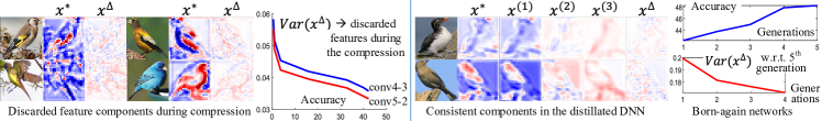
Network compression is an emerging research direction in recent years. Knowledge consistency between the compressed network and the original network can evaluate the discarding of knowledge during the compression process. I.e. people may visualize or analyze feature components in the original network, which are not consistent with features in the compressed network, to represent the discarded knowledge in the compressed network.
In experiments, we trained the VGG-16 using the CUB200-2011 dataset (Wah et al., 2011) for fine-grained classification. Then, we compressed the VGG-16 using the method of (Han et al., 2016) with different pruning thresholds. We used features of the compressed DNN to reconstruct features of the original DNN. Then, inconsistent components disentangled from the original DNN usually corresponded to the knowledge discarding during the compression process. Fig. 4(left) visualizes the discarded feature components. We used (defined in Section 4.2) to quantify the information discarding. Fig. 4 compares the decrease of accuracy with the discarding of feature information.
4.5 Explaining knowledge distillation via knowledge consistency
As a generic tool, our method can also explain the success of knowledge distillation. In particular, (Furlanello et al., 2018) proposed a method to gradually refine a neural network via recursive knowledge distillation. I.e. this method recursively distills the knowledge of the current net to a new net with the same architecture and distilling the new net to an even newer net. The new(er) net is termed a born-again neural network and learned using both the task loss and the distillation loss. Surprisingly, such a recursive distillation process can substantially boost the performance of the neural network in various experiments.
In general, the net in a new generation both inherits knowledge from the old net and learns new knowledge from the data. The success of the born-again neural network can be explained as that knowledge representations of networks are gradually enriched during the recursive distillation process. To verify this assertion, in experiments, we trained the VGG-16 using the CUB200-2011 dataset (Wah et al., 2011) for fine-grained classification. We trained born-again neural networks of another four generations333Because (Furlanello et al., 2018) did not clarify the distillation loss, we applied the distillation loss in (Hinton et al., 2014) following parameter settings in (Mishra & Marr, 2018), i.e. .. We disentangled feature components in the newest DNN, which were not consistent with an intermediate DNN. Inconsistent components were considered as blind spots of knowledge representations of the intermediate DNN and were quantified by . Fig. 4(right) shows of DNNs in the 1st, 2nd, 3rd, and 4th generations. Inconsistent components were gradually reduced after several generations.
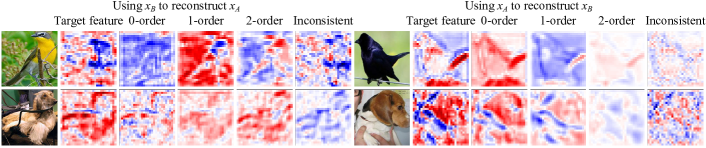
4.6 Consistent and inconsistent features between different tasks
In order to visualize consistent and inconsistent features between different tasks (i.e. the fine-grained classification and the binary classification), we trained DNN A (a VGG-16 network) to simultaneously classify 320 species, including 200 bird species in the CUB200-2011 dataset (Wah et al., 2011) and 120 dog species in the Stanford Dogs dataset (Khosla et al., 2011), in a fine-grained manner. On the other hand, we learned DNN B (another VGG-16 network) for the binary classification of the bird and the dog based on these two datasets. We visualized the feature maps of consistent and inconsistent feature components between the two DNNs in Fig. 5. Obviously, DNN A encoded more knowledge than DNN B, thereby reconstructing more features than .
5 Conclusion
In this paper, we have proposed a generic definition of knowledge consistency between intermediate-layers of two DNNs. A task-agnostic method is developed to disentangle and quantify consistent features of different orders from intermediate-layer features. Consistent feature components are usually more reliable than inconsistent components for the task, so our method can be used to further refine the pre-trained DNN without a need for additional supervision. As a mathematical tool, knowledge consistency can also help explain existing deep-learning techniques, and experiments have demonstrated the effectiveness of our method.
Acknowledgements
This work was partially supported by National Natural Science Foundation of China (U19B2043 and 61906120) and Huawei Technologies.
References
- Achille & Soatto (2018) Alessandro Achille and Stefano Soatto. Information dropout: learning optimal representations through noise. In Transactions on PAMI, 40(12):2897–2905, 2018.
- Arpit et al. (2017) Devansh Arpit, Stanislaw Jastrzebski, Nicolas Ballas, David Krueger, Emmanuel Bengio, Maxinder S. Kanwal, Tegan Maharaj, Asja Fischer, Aaron Courville, Yoshua Bengio, and Simon Lacoste-Julien. A closer look at memorization in deep networks. In ICLR, 2017.
- Bau et al. (2017) David Bau, Bolei Zhou, Aditya Khosla, Aude Oliva, and Antonio Torralba. Network dissection: Quantifying interpretability of deep visual representations. In CVPR, 2017.
- Bengio et al. (2014) Yoshua Bengio, Aaron Courville, and Pascal Vincent. Representation learning: A review and new perspectives. In arXiv:1206.5538v3, 2014.
- Chen et al. (2016) Xi Chen, Yan Duan, Rein Houthooft, John Schulman, Ilya Sutskever, and Pieter Abbeel. Infogan: Interpretable representation learning by information maximizing generative adversarial nets. In NIPS, 2016.
- Cheng et al. (2018) Hao Cheng, Dongze Lian, Shenghua Gao, and Yanlin Geng. Evaluating capability of deep neural networks for image classification via information plane. In ECCV, 2018.
- Deng et al. (2009) Jia Deng, Wei Dong, Richard Socher, Li-Jia Li, Kai Li, and Li Fei-Fei. Imagenet: A large-scale hierarchical image database. In CVPR, 2009.
- Deutsch (2018) Lior Deutsch. Generating neural networkswith neural networks. In arXiv:1801.01952, 2018.
- Dosovitskiy & Brox (2016) Alexey Dosovitskiy and Thomas Brox. Inverting visual representations with convolutional networks. In CVPR, 2016.
- Everingham et al. (2015) M. Everingham, S. M. A. Eslami, L. Van Gool, C. K. I. Williams, J. Winn, and A. Zisserman. The pascal visual object classes challenge: A retrospective. In International Journal of Computer Vision (IJCV), 111(1):98–136, 2015.
- Fong & Vedaldi (2018) Ruth Fong and Andrea Vedaldi. Net2vec: Quantifying and explaining how concepts are encoded by filters in deep neural networks. In CVPR, 2018.
- Fong & Vedaldi (2017) Ruth C. Fong and Andrea Vedaldi. Interpretable explanations of black boxes by meaningful perturbation. In ICCV, 2017.
- Fort et al. (2019) Stanislav Fort, Pawel Krzysztof Nowak, and Srini Narayanan. Stiffness: A new perspective on generalization in neural networks. In arXiv:1901.09491, 2019.
- Furlanello et al. (2018) Tommaso Furlanello, Zachary Lipton, Michael Tschannen, Laurent Itti, and Anima Anandkumar. Born again neural networks. In ICML, 2018.
- Guan et al. (2019) Chaoyu Guan, Xiting Wang, Quanshi Zhang, Runjin Chen, Di He, and Xing Xie. Towards a deep and unified understanding of deep neural models in nlp. In ICML, 2019.
- Han et al. (2016) Song Han, Huizi Mao, and William J. Dally. Deep compression: Compressing deep neural networks with pruning, trained quantization and huffman coding. In ICLR, 2016.
- He et al. (2016) Kaiming He, Xiangyu Zhang, Shaoqing Ren, and Jian Sun. Deep residual learning for image recognition. In CVPR, 2016.
- Higgins et al. (2017) Irina Higgins, Loic Matthey, Arka Pal, Christopher Burgess, Xavier Glorot, Matthew Botvinick, Shakir Mohamed, and Alexander Lerchner. -vae: learning basic visual concepts with a constrained variational framework. In ICLR, 2017.
- Hinton et al. (2014) Geoffrey Hinton, Oriol Vinyals, and Jeff Dean. Distilling the knowledge in a neural network. In NIPS Workshop, 2014.
- Huang et al. (2019) Shikun Huang, Binbin Zhang, Wen Shen, Zhihua Wei, and Quanshi Zhang. Utility analysis of network architectures for 3d point cloud processing. In arXiv:1911.09053, 2019.
- Khosla et al. (2011) Aditya Khosla, Nityananda Jayadevaprakash, Bangpeng Yao, and Li Fei-Fei. Novel dataset for fine-grained image categorization. In First CVPR Workshop on Fine-Grained Visual Categorization (FGVC), 2011.
- Kindermans et al. (2018) Pieter-Jan Kindermans, Kristof T. Schütt, Maximilian Alber, Klaus-Robert Müller, Dumitru Erhan, Been Kim, and Sven Dähne. Learning how to explain neural networks: Patternnet and patternattribution. In ICLR, 2018.
- Koh & Liang (2017) PangWei Koh and Percy Liang. Understanding black-box predictions via influence functions. In ICML, 2017.
- Kornblith et al. (2019) Simon Kornblith, Mohammad Norouzi, Honglak Lee, and Geoffrey Hinton. Similarity of neural network representations revisited. In arXiv:1905.00414, 2019.
- Krizhevsky et al. (2012) A. Krizhevsky, I. Sutskever, and G. E. Hinton. Imagenet classification with deep convolutional neural networks. In NIPS, 2012.
- Lakkaraju et al. (2017) Himabindu Lakkaraju, Ece Kamar, Rich Caruana, and Eric Horvitz. Identifying unknown unknowns in the open world: Representations and policies for guided exploration. In AAAI, 2017.
- Lundberg & Lee (2017) Scott M. Lundberg and Su-In Lee. A unified approach to interpreting model predictions. In NIPS, 2017.
- Ma et al. (2019) Haotian Ma, Yinqing Zhang, Fan Zhou, and Quanshi Zhang. Quantifying layerwise information discarding of neural networks. In arXiv:1906.04109, 2019.
- Mahendran & Vedaldi (2015) Aravindh Mahendran and Andrea Vedaldi. Understanding deep image representations by inverting them. In CVPR, 2015.
- Mishra & Marr (2018) Asit K. Mishra and Debbie Marr. Apprentice: Using knowledge distillation techniques to improve low-precision network accuracy. 2018.
- Montavon et al. (2011) Grégoire Montavon, Mikio L. Braun, and Klaus-Robert Müller. Kernel analysis of deep networks. In Journal of Machine Learning Research, 12:2563–2581, 2011.
- Morcos et al. (2018) Ari S. Morcos, Maithra Raghu, and Samy Bengio. Insights on representational similarity in neural networks with canonical correlation. In NIPS, 2018.
- Novak et al. (2018) Roman Novak, Yasaman Bahri, Daniel A. Abolafia, Jeffrey Pennington, and Jascha Sohl-Dickstein. Sensitivity and generalization in neural networks: An empirical study. In ICLR, 2018.
- Raghu et al. (2017) Maithra Raghu, Justin Gilmer, Jason Yosinski, and Jascha Sohl-Dickstein. Svcca: Singular vector canonical correlation analysis for deep learning dynamics and interpretability. In NIPS, 2017.
- Ribeiro et al. (2016) Marco Tulio Ribeiro, Sameer Singh, and Carlos Guestrin. “why should i trust you?” explaining the predictions of any classifier. In KDD, 2016.
- Sabour et al. (2017) Sara Sabour, Nicholas Frosst, and Geoffrey E. Hinton. Dynamic routing between capsules. In NIPS, 2017.
- Schwartz-Ziv & Tishby (2017) Ravid Schwartz-Ziv and Naftali Tishby. Opening the black box of deep neural networks via information. In arXiv:1703.00810, 2017.
- Selvaraju et al. (2017) Ramprasaath R. Selvaraju, Michael Cogswell, Abhishek Das, Ramakrishna Vedantam, Devi Parikh, and Dhruv Batra. Grad-cam: Visual explanations from deep networks via gradient-based localization. In ICCV, 2017.
- Simon & Rodner (2015) Marcel Simon and Erik Rodner. Neural activation constellations: Unsupervised part model discovery with convolutional networks. In ICCV, 2015.
- Simonyan & Zisserman (2015) Karen Simonyan and Andrew Zisserman. Very deep convolutional networks for large-scale image recognition. In ICLR, 2015.
- Szegedy et al. (2014) Christian Szegedy, Wojciech Zaremba, Ilya Sutskever, Joan Bruna, Dumitru Erhan, Ian Goodfellow, and Rob Fergus. Intriguing properties of neural networks. In arXiv:1312.6199v4, 2014.
- Wah et al. (2011) C. Wah, S. Branson, P. Welinder, P. Perona, and S. Belongie. The caltech-ucsd birds-200-2011 dataset. Technical report, In California Institute of Technology, 2011.
- Wang et al. (2018) Liwei Wang, Lunjia Hu, Jiayuan Gu, Yue Wu, Zhiqiang Hu, Kun He, and John Hopcroft. Towards understanding learning representations: To what extent do different neural networks learn the same representation. In NIPS, 2018.
- Wolchover (2017) Natalie Wolchover. New theory cracks open the black box of deep learning. In Quanta Magazine, 2017.
- Xu & Raginsky (2017) Aolin Xu and Maxim Raginsky. Information-theoretic analysis of generalization capability of learning algorithms. In NIPS, 2017.
- Yosinski et al. (2014) Jason Yosinski, Jeff Clune, Yoshua Bengio, and Hod Lipson. How transferable are features in deep neural networks? In NIPS, 2014.
- Zeiler & Fergus (2014) Matthew D. Zeiler and Rob Fergus. Visualizing and understanding convolutional networks. In ECCV, 2014.
- Zhang et al. (2017) Chiyuan Zhang, Samy Bengio, Moritz Hardt, Benjamin Recht, and Oriol Vinyals. Undersantding deep learning requires rethinking generalization. In ICLR, 2017.
- Zhang et al. (2019) Hao Zhang, Jiayi Chen, Haotian Xue, and Quanshi Zhang. Towards a unified evaluation of explanation methods without ground truth. In arXiv:1911.09017, 2019.
- Zhang et al. (2018a) Quanshi Zhang, Wenguan Wang, and Song-Chun Zhu. Examining cnn representations with respect to dataset bias. In AAAI, 2018a.
- Zhang et al. (2018b) Quanshi Zhang, Ying Nian Wu, and Song-Chun Zhu. Interpretable convolutional neural networks. In CVPR, 2018b.
- Zhou et al. (2015) Bolei Zhou, Aditya Khosla, Agata Lapedriza, Aude Oliva, and Antonio Torralba. Object detectors emerge in deep scene cnns. In ICLR, 2015.
- Zhou et al. (2018) Bolei Zhou, Yiyou Sun, David Bau, and Antonio Torralba. Interpretable basis decomposition for visual explanation. In ECCV, 2018.
Appendix A Fairness of experiments in Section 4.3
In Section 4.3, we used knowledge consistency to refine intermediate-layer features of pre-trained DNNs. Given multiple DNNs pre-trained for the same task, feature components, which are consistent with various DNNs, usually represent common knowledge and are reliable. In this way, intermediate-layer features can be refined by removing inconsistent components and exclusively using consistent components to accomplish the task.
Both Experiment 1 and Experiment 2 followed the same procedure. I.e. we trained two DNNs and for the same task. Then, we extracted consistent feature components when we used the DNN ’s feature to reconstruct the DNN ’s feature. We compared the classification performance of the DNN , the DNN , and the classifier learned based on consistent features .
However, an issues of fairness may be raised, i.e. when we added the network upon the DNN , this operation increased the depth of the network. Thus, the comparison between the revised DNN and the original DNN may be unfair.
In order to ensure a fair comparison, we applied following experimental settings.
For the evaluation of DNNs and , both the DNNs were further refined using target training samples in Experiments 1 and 2.
For the evaluation of our method, without using any annotations of the target task, we first trained to use to reconstruct and disentangle consistent feature components. Then, we fixed all parameters of DNNs , , and , and only used output features of to train a classifier, in order to test the discrimination power of output features of .
![[Uncaptioned image]](/html/1908.01581/assets/x6.png)
As shown in the above figure, for the evaluation of our method, first, we were not given any training annotations for the target task. Without any prior knowledge of the target task, we used the pre-trained DNNs (blue area in the above figure) to train the network (red area in the above figure). Then, we fixed parameters of DNNs in both red area and blue area in the above figure. Finally, we received training samples of the target task, and used them to exclusively train the classifier (the blue area in the above figure).
In short, the learning of the network was independent with the target task, and parameters of , , and were not refine-tuned during the learning of the new classifier.
Appendix B Blind spots and unreliable features
By our assumption, strong DNNs can encode true knowledge, while there are more representation flaws in weak DNNs. If we try to use the intermediate features of a weak DNN to reconstruct intermediate features of a strong DNN, the strong DNN features cannot be perfectly reconstructed due to the inherent blind spots of the weak DNN. On the other hand, when we use features of a strong DNN to reconstruct a weak DNN’s features, the unreconstructed feature components in these reconstructed features also exist. These unreconstructed parts are not modeled in the strong DNN, and they are termed unreliable features by us.