The HSIC Bottleneck: Deep Learning without Back-Propagation

Abstract

We introduce the HSIC (Hilbert-Schmidt independence criterion) bottleneck for training deep neural networks. The HSIC bottleneck is an alternative to the conventional cross-entropy loss and backpropagation that has a number of distinct advantages. It mitigates exploding and vanishing gradients, resulting in the ability to learn very deep networks without skip connections. There is no requirement for symmetric feedback or update locking. We find that the HSIC bottleneck provides performance on MNIST/FashionMNIST/CIFAR10 classification comparable to backpropagation with a cross-entropy target, even when the system is not encouraged to make the output resemble the classification labels. Appending a single layer trained with SGD (without backpropagation) to reformat the information further improves performance.

1 Introduction

Deep learning has brought a new level of performance to an increasingly wide range of tasks. In practice however, the stochastic gradient descent (SGD) algorithm (and its variants) and the associated error back-propagation algorithm underlying deep learning are time consuming, have problems of vanishing and exploding gradients, require sequential computation across layers and update locking, and typically require the exploration of learning rates and other hyperparameters. At the same time, backpropagation is generally regarded as being not biologically plausible. These considerations are driving research into both theoretical and practical alternatives.

We propose a deep network training method that does not use the cross-entropy loss or backpropagation. An alternate information-theoretic motivation of training a classifier can be found in terms of the Fano inequality and mutual information. In our context, Fano’s inequality indicates that the probability of classification error depends on the conditional entropy $H(Y|X)$, with $Y$ being the label and $X$ some representation of the input. Additionally, the mutual information $I(X,Y)$ can be written in the form $I(X,Y)=H(Y)-H(Y|X)$. Note that the entropy of the labels is constant with respect to the network weights. When the probability of mis-classification is low, $H(Y|X)$ is also low, and the mutual information is high. Mutual information thus provides a training objective that directly involves the representation $X$, unlike cross entropy, which involves $X$ only through backpropagation.

As is the case with cross entropy, an algorithm trained exclusively using mutual information is vulnerable to overfitting. To address this we train the network using an approximation of the information bottleneck (?). Due to the practical difficulties of calculating the mutual information among the random variables, we adopt a non-parametric kernel-based method, the Hilbert-Schmidt independence criterion (HSIC), to characterize the statistical (in)dependence of different layers. That is, for each network layer we maximize HSIC between the layer activation and the desired output and minimize HSIC between that layer activation and the input. In some cases, the final-layer representations resulting from this HSIC bottleneck training are nearly one-hot and can be directly used for classification after identifying a single fixed permutation. Alternately, following HSIC bottleneck training, we append a single classification layer that is trained with SGD (without backpropagation), consistently obtaining performance competitive with an architecturally equivalent network trained with backpropagation. We provide an informal discussion of the relation between HSIC and mutual information in the Appendix.

Our work joins an increasing body of recent research that explores deep learning fundamentals from an information theoretical perspective ((?; ?; ?; ?) and others). Our contributions are as follows:

We demonstrate that it is possible to train deep classification networks using an information bottleneck principle, without backpropagation, and obtain results competitive with the standard backpropagation optimization of the cross-entropy objective. The HSIC bottleneck approach mitigates the issue of vanishing or exploding gradients in backpropagation. As the HSIC-bottleneck operates directly on continuous random variables, it is more attractive than conventional information bottleneck approaches based on binning. Because the network training is explicitly based on an information bottleneck principle, it addresses overfitting by design. It further addresses the weight transport and update locking problems of backpropagation.

The experimental results demonstrate training several simple textbook architectures using the HSIC bottleneck, together with the results of the otherwise identical architecture trained with backpropagation. However, note that the backpropagation results require an additional final layer and softmax that is not required nor used in the “unformatted” HSIC-training case. While the results provide a fair comparison, there was no exploration of alternative architectures, regularization, or data augmentation, and relatively little effort towards finding optimal hyperparameters. Thus neither the backpropagation baseline nor our method give state-of-the-art results, and further improvements are likely possible.

Notation. Upper case (e.g., $X,Y$) denotes random variables. Bold denotes vectors of observations (lower case, e.g., $\mathbf{x},\mathbf{y}$) or matrices (e.g., $\mathbf{H},\mathbf{K}$). Hilbert spaces are denoted with calligraphic font (e.g., $\mathcal{G},\mathcal{H}$).

2 Background and Related Work

Although SGD using the backpropagation algorithm (?) is the predominant approach to optimizing deep neural nets, other approaches have been considered (?; ?; ?; ?; ?). Kickback (?) follows the local gradient using a direction obtained from the global single-class error. Feedback alignment (?) shows that deep neural networks can be trained using random feedback connections. The alternating minimization (?), a coordinate descent-like approach, breaks the nested objective into a collection of subproblems by introducing auxiliary variables, thereby allowing layer-parallel updates.

Information theory (?) underlies much research on learning theory (?; ?; ?) as well as thinking in neuroscience (?). The information bottleneck (IB) principle (?) generalizes the notion of minimal sufficient statistics, expressing a tradeoff in the hidden representation between the information needed for predicting the output, and the information retained about the input. The IB objective is

$$\min_{p_{T_{i}|X}}I(X;T_{i})-\beta I(T_{i};Y),$$ (1)

where $X$, $Y$ are the input and label random variable respectively, and $T_{i}$ represents the hidden representation at layer $i$. Intuitively, the IB principal preserves the information of the hidden representations about the label while compressing information about the input data.

The IB principle has been employed both to explore deep learning dynamics and as a training objective in a growing body of recent work (?; ?; ?; ?; ?; ?; ?; ?) and others.

In practice, the IB is hard to compute for several reasons. If the network inputs are regarded as continuous, the mutual information $I(X,T_{i})$ is infinite unless noise is added to the network. Many algorithms are based on binning, which suffers from the curse of dimensionality and yields different results with different choices of bin size. The distinction between discrete and continuous data, and between discrete and differential entropy, presents additional considerations (?; ?). These issues are clearly surveyed in (?). In the case of continuous variables and a deterministic network, the true MI is infinite, while discrete data results in a piecewise-constant MI that is also unsuited for optimization. Existing approaches to applying IB to DNN learning have resorted to MI approximations such as adding noise and computing a bound rather than the actual quantity. However tighter bounds may not be better (?). It has been argued that the IB has inherent problems when applied to deep neural nets, and that current results may reflect the approximations to MI and inductive biases of the networks more than the true underlying mutual information (?; ?).

In this paper, we replace the mutual information terms in the information bottleneck objective with HSIC. In contrast to mutual information based estimates, HSIC provides a robust computation with a time complexity $O(m^{2})$ where $m$ is the number of data points. HSIC (?) is the Hilbert-Schmidt norm of the cross-covariance operator between the distributions in Reproducing Kernel Hilbert Space (RKHS). The formulation of HSIC is:

$$\begin{split}\text{HSIC}(\mathbb{P}_{XY},\mathcal{H},&\mathcal{G})=\left\|C_{XY}\right\|^{2}\\ &=\mathbb{E}_{XYX^{\prime}Y^{\prime}}[k_{X}(X,X^{\prime})k_{Y^{\prime}}(Y,Y^{\prime})]\\ &+\mathbb{E}_{XX^{\prime}}[k_{X}(X,X^{\prime})]\mathbb{E}_{Y^{\prime}}[k_{Y}(Y,Y^{\prime})]\\ &-2\mathbb{E}_{XY}[\mathbb{E}_{X^{\prime}}[k_{X}(X,X^{\prime})]\mathbb{E}_{Y^{\prime}}[k_{Y}(Y,Y^{\prime})]],\end{split}$$ (2)

where $k_{X}$ and $k_{Y}$ are kernel functions, $\mathcal{H}$ and $\mathcal{G}$ are the Hilbert spaces, and $\mathbb{E}_{XY}$ is the expectation over $X$ and $Y$.

Let $\mathcal{D}:=\{(\mathbf{x}_{1},\mathbf{y}_{1}),\cdots,(\mathbf{x}_{m},\mathbf{y}_{m})\}$ contain $m$ i.i.d. samples drawn from $\mathbb{P}_{XY}$, where $\mathbf{x}_{i}\in\mathbb{R}^{d_{x}}$ and $\mathbf{y}_{i}\in\mathbb{R}^{d_{y}}$. Then (2) leads to the following empirical expression (?):

$$\text{HSIC}(\mathcal{D},\mathcal{H},\mathcal{G})=(m-1)^{-2}\operatorname{tr}(\mathbf{K}_{X}\mathbf{H}\mathbf{K}_{Y}\mathbf{H})$$ (3)

where $\mathbf{K}_{X}\in\mathbb{R}^{m\times m}$ and $\mathbf{K}_{Y}\in\mathbb{R}^{m\times m}$ have entries ${\mathbf{K}_{X}}_{ij}=k(\mathbf{x}_{i},\mathbf{x}_{j})$ and ${\mathbf{K}_{Y}}_{ij}=k(\mathbf{y}_{i},\mathbf{y}_{j})$, and $\mathbf{H}\in R^{m\times m}$ is the centering matrix $\mathbf{H}=\mathbf{I}_{m}-\frac{1}{m}\textbf{1}_{m}\textbf{1}_{m}^{T}$.

With an appropriate kernel choice such as the Gaussian $k(\mathbf{x},\mathbf{y})\sim\exp(-\frac{1}{2}\|\mathbf{x}-\mathbf{y}\|^{2}/\sigma^{2})$, HSIC is zero if and only if the random variables $X$ and $Y$ are independent, $P_{XY}=P_{X}P_{Y}$ (?). An intuition for the HSIC approach is provided by the fact that the series expansion of the exponential contains a weighted sum of all moments of the data, and (under reasonable conditions) two distributions are equal if and only if their moments are identical. Considering the expression (3), the i’th of component of (3) is

$$\langle{k_{X}}_{i,1},\,{k_{X}}_{i,2},\,\cdots,{k_{X}}_{i,n}\rangle\cdot\langle{k_{Y}}_{1,i},\,{k_{Y}}_{2,i},\,\cdots,{k_{Y}}_{n,i}\rangle$$ (4)

where ${k_{X}}_{i,j}\equiv(\mathbf{K}_{X}\mathbf{H})_{i,j}$ and similarly ${k_{Y}}_{i,j}\equiv(\mathbf{K}_{Y}\mathbf{H})_{i,j}$. This inner product will be large when the relation between each point $i$ of $X$ and all other points of $X$ is similar to the relation between the corresponding point $i$ of $Y$ and all other points of $Y$, summed over all $i$, and where similarity is measured through the kernel $k(x_{i},x_{j})$ that (appropriately chosen) captures all statistical moments of the data.

In our experiments we use the normalized-HSIC (nHSIC) formulation based on the normalized cross-covariance operator (?; ?), given by:

$$\text{nHSIC}(\mathcal{D},\mathcal{H},\mathcal{G})=\operatorname{tr}(\widetilde{\mathbf{K}}_{X}\widetilde{\mathbf{K}}_{Y})$$ (5)

where $\widetilde{\mathbf{K}}_{X}=\overline{\mathbf{K}}_{X}\left(\overline{\mathbf{K}}_{X}+\epsilon m\mathbf{I}_{m}\right)^{-1}$ and $\widetilde{\mathbf{K}}_{Y}=\overline{\mathbf{K}}_{Y}\left(\overline{\mathbf{K}}_{Y}+\epsilon m\mathbf{I}_{m}\right)^{-1}$. $\overline{\mathbf{K}}_{X}$ and $\overline{\mathbf{K}}_{Y}$ denote centered kernel matrices, and $\epsilon$ is a small constant.

Unlike mutual information, HSIC does not have an interpretation in terms of information theoretic quantities (bits or nats). On the other hand, HSIC does not require density estimation and is simple and reliable to compute. Moreover, kernel distribution embedding approaches such as HSIC can also be resistant to outliers, as can be seen by considering the effect of outliers under the Gaussian kernel. The empirical estimate converges to the population HSIC value at the rate $1/\sqrt{n}$ independent of the dimensionality of the data (?), meaning that it partially circumvents the curse of dimensionality.

HSIC is widely used as a dependency measurement, including in the deep learning literature. For example, (?) investigated the generalization properties of autoencoders using HSIC, while (?) uses HSIC to restrict the latent space search to constrain the aggregate variational posterior. (?) use distance correlation (an alternate formulation of HSIC) to remove unnecessary private information from medical training data.

While in principle HSIC can discover arbitrary dependencies between variables, in practice and with finite data the choice of the $\sigma$ parameter in the HSIC kernel emphasizes relationships at some scales more than others. Intuitively, two data points $x,y$ are not well distinguished when their difference is sufficiently small or large, such that they lie on the small-slope portions of the Gaussian. This is typically handled by choosing the kernel $\sigma$ based on median distances among the data (?; ?), or by a hyperparameter search.

In our case, the data “points” are minibatches of activations from different network layers, and thus have different dimensionality. This suggests that different $\sigma$ values should be used in each kernel. Using the observation that the expected squared distance between random points scales with dimension, these multiple hyperparameters can be approximated by scaling a single $\sigma$ with the dimensionality $d$ of points $\mathbf{x}$ and $\mathbf{y}$ as: $k(\mathbf{x},\mathbf{y})\sim\exp(-\frac{1}{2}\|\mathbf{x}-\mathbf{y}\|^{2}/(\sigma^{2}d))$ (used in all our experiments).

3 Proposed Method

In this section we introduce the proposed HSIC-trained network. Training a deep network without backpropagation using the HSIC-bottleneck objective will be generally termed HSIC-bottleneck training or HSIC-training. The output of the bottleneck-trained network contains the information necessary for classification, but not necessarily in the right form. We evaluate two specific approaches to produce classifications from the HSIC-bottleneck trained network. First, if the outputs are one-hot, they can simply be permuted to align with the training labels. This is termed unformatted-training. In the second scheme, we append a single layer and softmax output to the frozen unformatted-trainednetwork, and train the appended layer using SGD without backpropagation. Since this step is “reformatting” the information, this step is termed format-training. Note that the networks trained with backpropagation contain this softmax layer in every case.

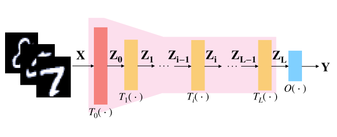
(a) HSIC-trained Network

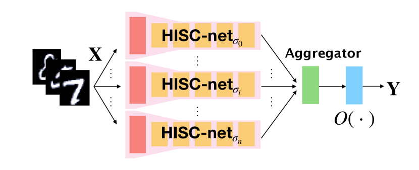
(b) multiple-scale network

Figure 1: The HSIC-trained network (Fig. 1(a)) is a standard feedforward network trained using the HSIC-bottleneck objective, resulting in hidden representations at the last layer that can easily be used for classification. Fig. 1(b) shows a multiple-scale network, where each branch $\text{HSIC-net}_{\sigma_{j}}$ is trained with a specific $\sigma$. The aggregator averages the hidden representations to form an output representation.

3.1 HSIC-Bottleneck

Suppose we have a network composed of $L$ hidden layers $T_{i}(\cdot):\mathbb{R}^{d_{i-1}}\rightarrow\mathbb{R}^{d_{i}}$, resulting in hidden representations $\mathbf{Z}_{i}\in\mathbb{R}^{m\times d_{i}}$, where $i\in\{1,...,L\}$, and $m$ denotes batch size. Implementing the Information Bottleneck principle, we replace the original mutual information terms with nHSIC (5) as the learning objective:

$$\mathbf{Z}_{i}^{\ast}=\operatorname*{arg\,min}_{\mathbf{Z}_{i}}\ \text{nHSIC}(\mathbf{Z}_{i},\mathbf{X})-\beta\,\text{nHSIC}(\mathbf{Z}_{i},\mathbf{Y}),$$ (6)

where $\mathbf{X}\in\mathbb{R}^{m\times d_{x}}$ is the input, $\mathbf{Y}\in\mathbb{R}^{m\times d_{y}}$ is the label, $i\in\{0,...,L\}$ and $L$ is the number of hidden layers, $d_{x}$ and $d_{y}$ are the dimensionalities of the input and output variables respectively. Since we concentrate on classification in our experiments, $d_{y}$ is the number of classes (we expect the HSIC bottleneck approach can be applied to other tasks such as regression). The $\beta$ controls the balance of IB objectives. Following nHSIC of (5), the nHSIC of each term is:

$$\begin{split}\text{nHSIC}(\mathbf{Z}_{i},\mathbf{X})=\operatorname{tr}(\widetilde{\mathbf{K}}_{Z_{i}}\widetilde{\mathbf{K}}_{X})\\ \text{nHSIC}(\mathbf{Z}_{i},\mathbf{Y})=\operatorname{tr}(\widetilde{\mathbf{K}}_{Z_{i}}\widetilde{\mathbf{K}}_{Y})\end{split}$$ (7)

The formulation (6), (7) suggests that the optimal hidden representation $\mathbf{Z}_{i}$ finds a balance between independence from unnecessary details of the input and dependence with the output. Ideally, the information needed to predict the label is retained when (6) converges, while unnecessary information that would permit overfitting is removed.

We optimize equation (6) independently at each layer using block coordinate descent without gradient propagation.

Data: $\mathbf{X}_{j}\in\mathbb{R}^{m\times d_{x}}$: data batch $j$, $\mathbf{Y}_{j}\in\mathbb{R}^{m\times d_{y}}$: label batch $j$, layer $T_{i}$ parameterized by $\{\bm{\theta}_{i}|\mathbf{W}_{i},\mathbf{b}_{i}\}$, $i\in\{1,...,L\}$: layer iterator, $j\in\{1,...,\lfloor n/m\rfloor\}$: batch iterator, $m$: batch size, $n$: number of input data, $\alpha$: learning rate.

Result: Saved HSIC-trained network $T_{i}(\cdot):\mathbb{R}^{d_{i-1}}\rightarrow\mathbb{R}^{d_{i}}$, $i\in\{1,...,L\}$

for $j\in\{1,...,n/m\}$ do

       for $i\in\{1,...,L\}$ do

             $\mathbf{Z}_{i}=\mathbf{T}_{i-1}(\mathbf{Z}_{i-1})$        // $\mathbf{Z}_{0}=\mathbf{X}_{j}$

             $\mathbf{g}_{i}=\nabla_{\bm{\theta}_{i}}(\text{nHSIC}(\mathbf{Z}_{i},\mathbf{X}_{j})-\beta\text{nHSIC}(\mathbf{Z}_{i},\mathbf{Y}_{j}))$

             $\bm{\theta}_{i}\leftarrow\bm{\theta}_{i}-\alpha\mathbf{g}_{i}$

            

       end for

      

end for

Algorithm 1 Unformatted training

3.2 Unformatted training

As shown in the Experiments section, HSIC-bottleneck training tends to produce one-hot outputs in some experiments. This inspired us to use the HSIC-bottleneck objective to directly solve the classification problem. This is done by setting the dimensionality of the last layer $\mathbf{Z}_{L}$ to match the number of classes (e.g., $d_{L}=d_{y}$). Since the resulting activation is typically permuted with respect to the labels (e.g., images of the digit zero might activate the forth output layer entry), we simply find a fixed permutation by picking the output with the highest activation across the inputs of a particular class as the output for that class. Please refer to Algorithm 1 for more detail.

3.3 Format-trained network

We append a single output layer $O(\cdot):\mathbb{R}^{d_{L}}\rightarrow\mathbb{R}^{d_{y}}$ equipped with a softmax function for classification (Fig. 1), taking the optimized last-layer hidden representation from a unformatted-trained network as its input. The new layer is trained using minibatch SGD with the loss

$$L_{\text{format}}=\text{CE}\big{(}\mathbf{Y},O(\mathbf{Z}_{L})\big{)}$$

where CE denotes the cross entropy loss.

3.4 Multiple-scale network

In principle, HSIC is a powerful measure of statistical independence, however in practice the results do depend somewhat on the chosen $\sigma$ parameter even when using the normalized form (5). To cope with this, we combine unformatted-trained networks with different $\sigma$, and then aggregate the resulting hidden representations. This multiple-scale network architecture is illustrated in Fig. 1(b), and has the objective

$$L_{\text{Comb}}(\mathbf{X},\mathbf{Y})=\text{CE}\bigg{(}{\mathbf{Y},O\big{(}\frac{1}{n}\sum_{i}^{n}\text{HSIC-net}_{\sigma_{i}}(\mathbf{X})\big{)}}\bigg{)}$$

where the output classifier layer $O(\cdot)$ takes the average of representations from the unformatted-trained networks, $\text{HSIC-net}_{\sigma_{i}}$, trained with $\sigma_{i}$, $i\in\{1,...,n\}$. Then it optimizes the layer $O(\cdot)$ with cross entropy while keeping the trained $\text{HSIC-net}_{\sigma_{i}}$ fixed. The performance of the multiple-scale network is presented below in Section 4.3.

3.5 Performance

Performance comparisons with backpropagation are difficult since the HSIC bottleneck performance depends heavily on the minibatch size. SGD backpropagation schemes are linear in the number of data points. HSIC is $O(m^{2})$ where $m$ is the minibatch size in our case. Typically the minibatch size is a constant that is chosen based on validation performance and/or available GPU memory rather than scaling with the data, so strictly speaking the HSIC-bottleneck approach is also linear in the number of data points. However, the learning convergence is a quantity of ultimate interest. This quantity is not known for either backpropagation or HSIC bottleneck, and it may be different considering the fundamentally distinct character of these two approaches. HSIC bottleneck is more amenable to layer parallel computation, since the need for backpropagation is removed.

4 Experiments

In this section, we report several experiments that explore and validate the HSIC-trained network concept. First, to motivate our work, we plot the HSIC-bottleneck values and activation distributions of a simple model during backpropagation training. We then show how unformatted-training can produce one-hot results that are directly ready for classification with a shallow or deep network. Next, we compare backpropagation with format-training on networks with different numbers of layers. The value of HSIC-training for format-training and the effect of the hyperparameter $\sigma$ are considered in the next experiments. Lastly, we briefly consider the application of HSIC-training to other network architectures such as ResNet.

For the experiments, we used standard feedforward networks with batch-normalization (?) on the MNIST/Fashion MNIST/CIFAR10 datasets. All experiments including standard backpropagation, unformatted-trained, and format-trained, use a simple SGD optimizer. The coefficient $\beta$ and the kernel scale factor $\sigma$ of the HSIC-bottleneck were set to 500 and 5 respectively, which empirically balances compression and the relevant information available for the classification task.

Before considering the use of the HSIC-bottleneck as a training objective, we first validate its relevance in the context of conventional deep network training (Fig. 2). Monitoring the nHSIC between hidden activations and the input and output of a simple network trained using backpropagation shows that $\text{nHSIC}(\mathbf{Y},\mathbf{Z}_{L})$ rapidly increased during early training as representations are formed, while $\text{nHSIC}(\mathbf{X},\mathbf{Z}_{L})$ rapidly drops. The value of $\text{nHSIC}(\mathbf{Y},\mathbf{Z}_{L})$ varies with the network depth (Fig. 2(e)) and depends on the choice of activation (Fig. 2(b)). Furthermore, it clearly parallels the increase in training accuracy (Fig. 2(c), Fig. 2(f)). In summary, Fig. 2 shows that a range of different networks follow the information bottleneck principal.

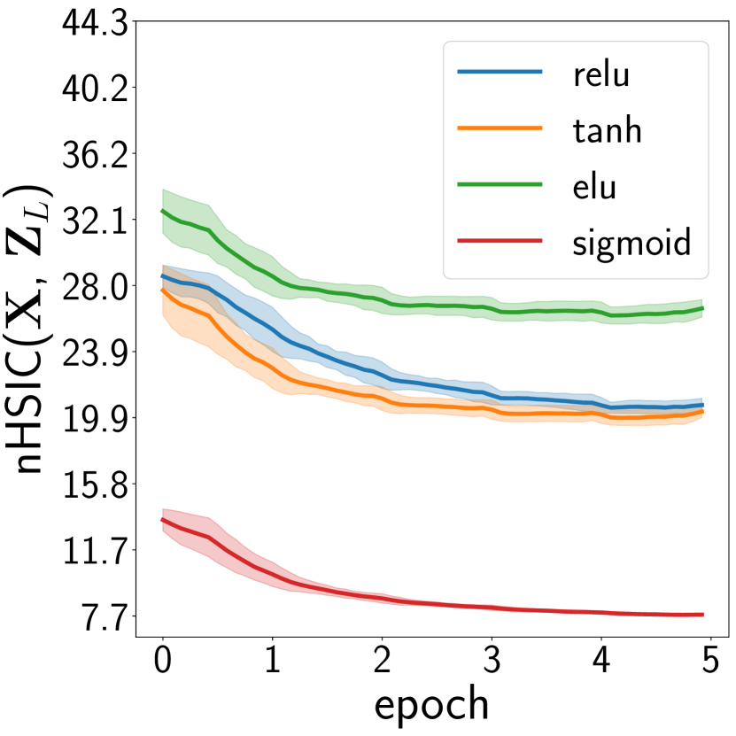
(a)

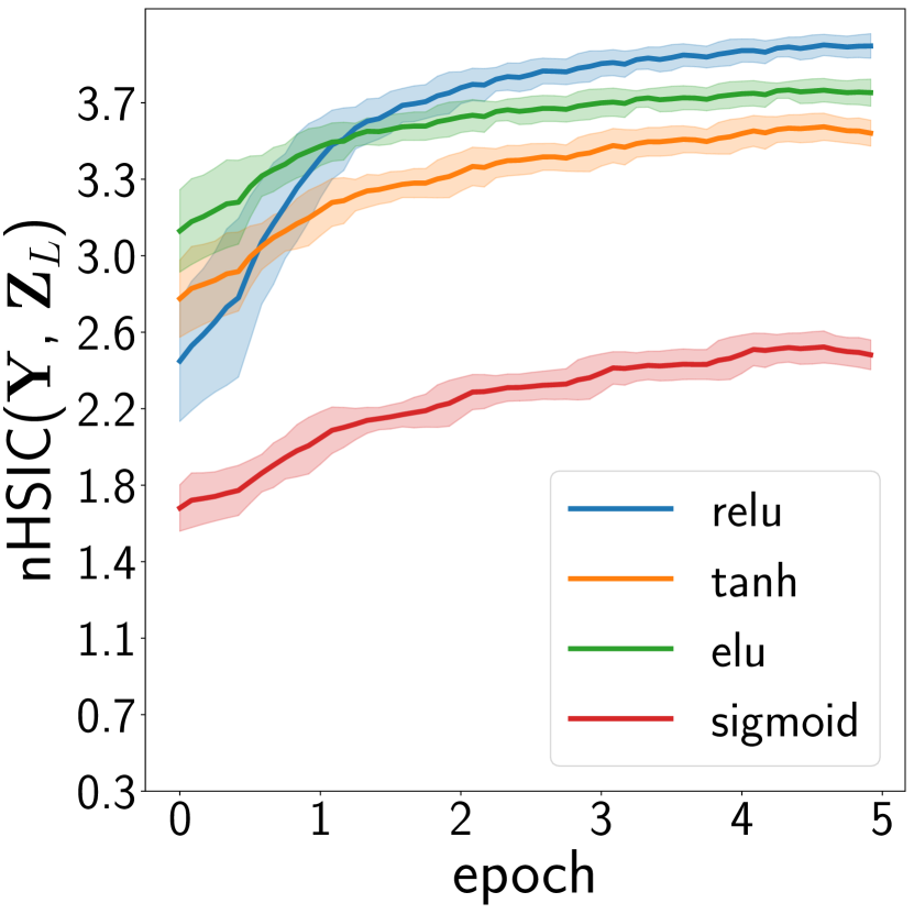
(b)

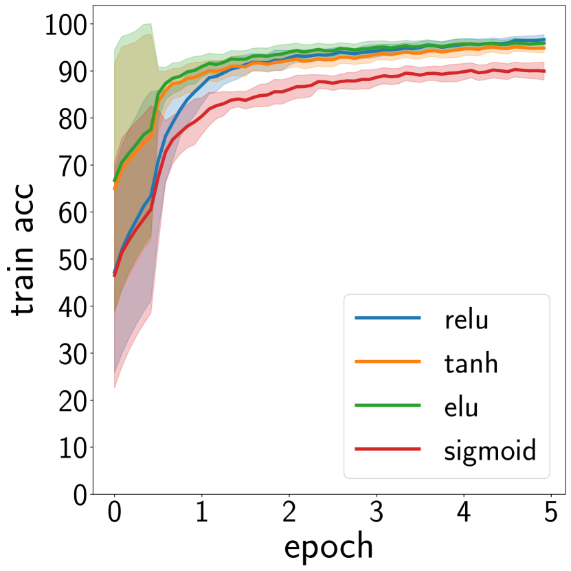
(c)

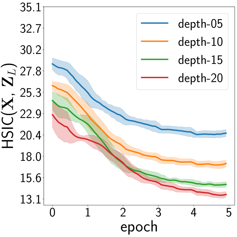
(d)

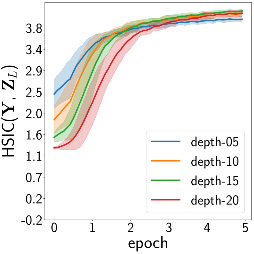
(e)

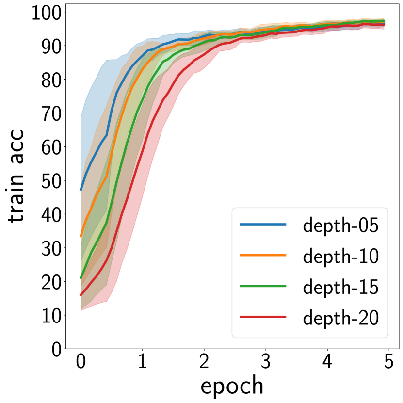
(f)

Figure 2: Visualization of the HSIC-bottleneck quantities $\text{nHSIC}(\mathbf{X},\mathbf{Z}_{L})$, $\text{nHSIC}(\mathbf{Y},\mathbf{Z}_{L})$ and training accuracy as a function of epoch number, monitored during conventional backpropagation training across various network activation functions Figs. (2(a))-(2(c)) and depths Figs. (2(d))-(2(f)). Figs. (2(d))-(2(f)) use ReLU with different network depths. Figs. (2(a))–(2(c)) vary only the activation type. The shaded area in the plots represents the standard deviation of the unsmoothed training performance.

4.1 Unformatted training

Next, we try using the HSIC-bottleneck as the sole training objective. We use a fully connected network architecture 784-256-256-256-256-256-10 with ReLU activation functions. Remarkably, in experiments on CIFAR10, FashionMNIST, and MNIST, the HSIC-trained network often results in non-overlapping one-hot output activations for many (but not all) random weight initializations, as seen in Fig. 3. This allows classification to be performed by simply using a fixed permutation, i.e., using the highest activation distribution value to select the class. For example in Fig. 3, the class activities of MNIST dataset from digit zero to nine have highest density at entries: 7, 6, 5, 4, 3, 2, 8, 1, 0, 9. We also tested a toy model to show that a network trained with unformatted-training can separate classes in a $\mathbb{R}^{1}$ latent space. More detail on this experiment is shown in the Appendix.

Our approach can produce results competitive with standard training. Fig. 4 illustrates the result for both backpropagation and unformatted-training for otherwise identical networks. We see that unformatted-training provides comparable results to backpropagation when the network is shallow (top-row); however, the performance of backpropagation is poor for deep networks (bottom-row). Note that the CIFAR10 results use a fully connected rather than convolutional network.

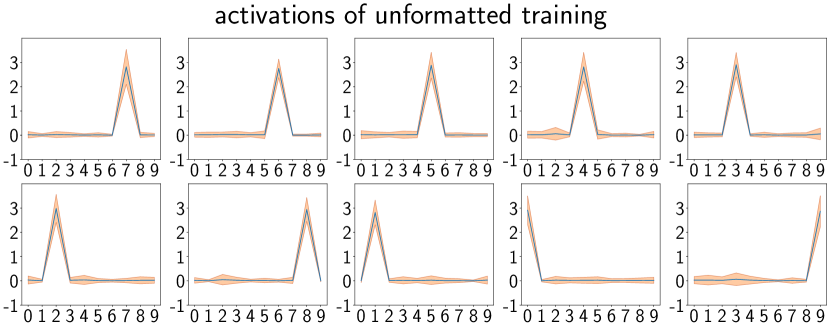
Figure 3: The MNIST output category distribution for a shallow fully-connected network. Each of the subfigures is the output for a specific category, from the ‘zero’ digits (top-left) to the ‘nine’ digits (bottom right). The zero inputs produced a one-hot activation in position seven, and the nines produces a one-hot activation in position nine, respectively. The particular permutation depends on the random weight initialization.

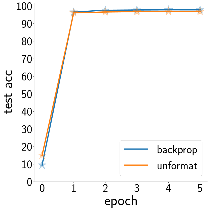
(a) MNIST

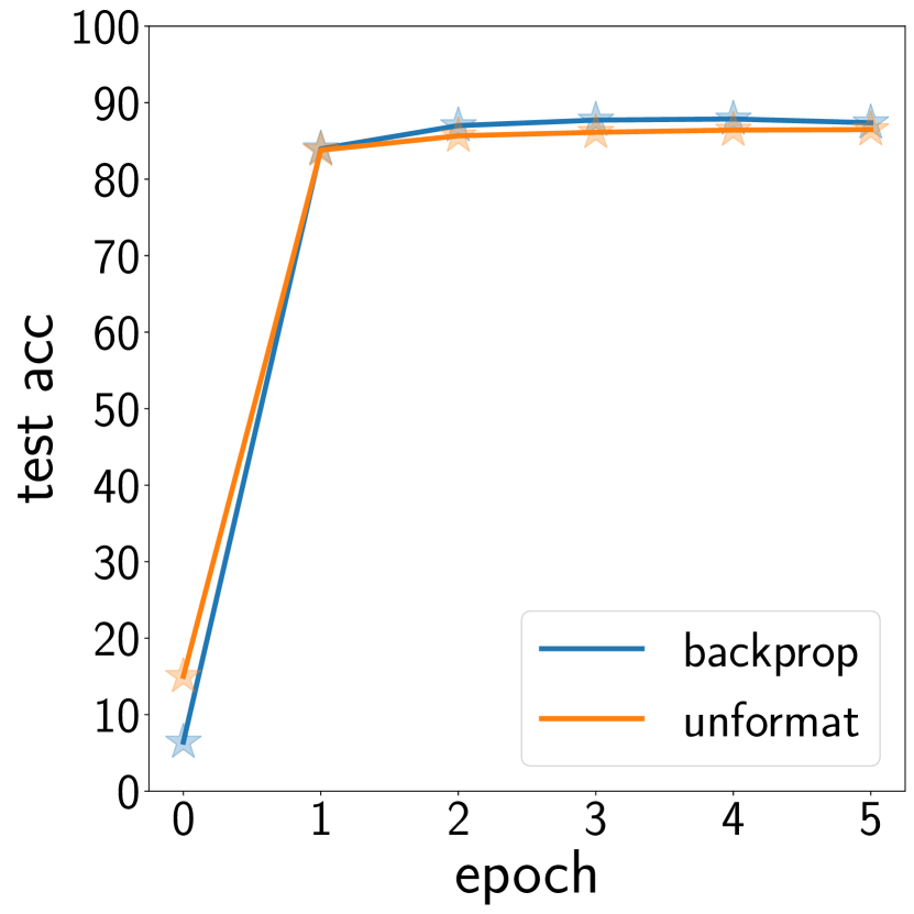
(b) FashionMNIST

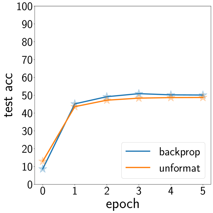
(c) CIFAR10

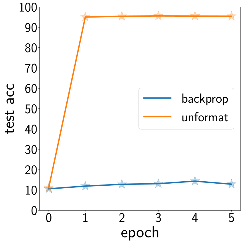
(d) MNIST

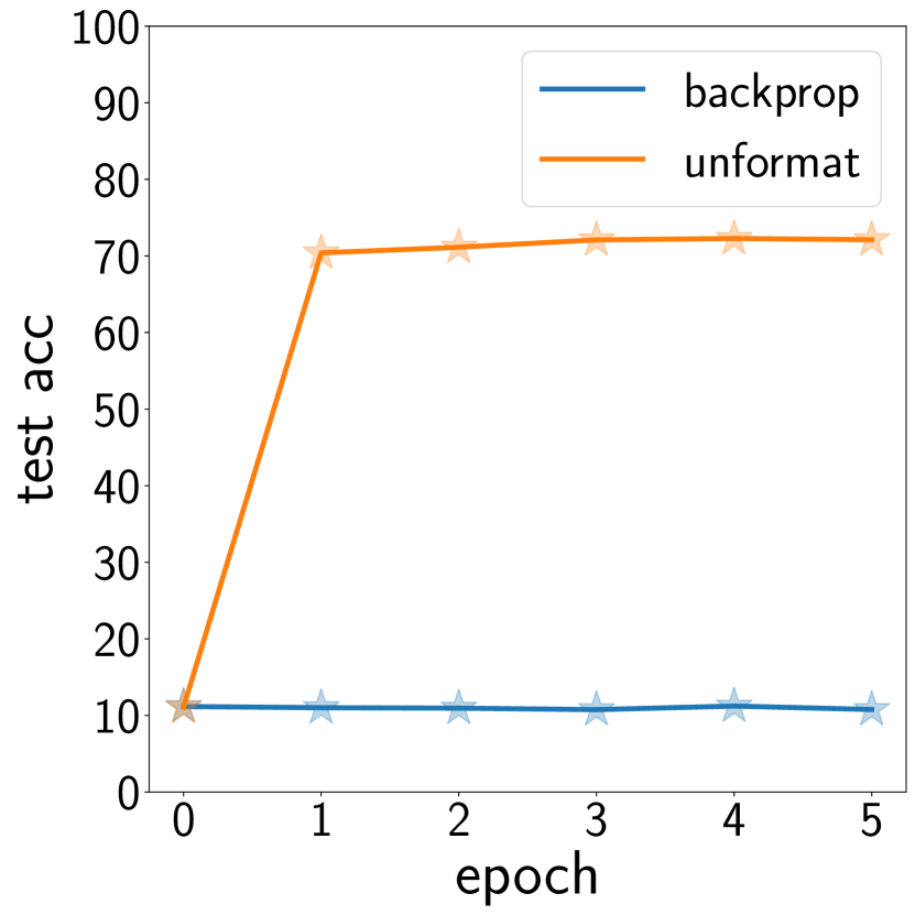
(e) FashionMNIST

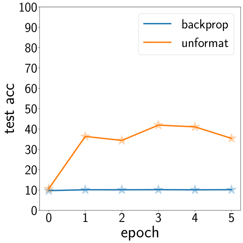
(f) CIFAR10

Figure 4: The test accuracy of HSIC-bottleneck training on standard classification problems as a function of epoch number. The experiments use the same architecture where the top- and bottom-row use 5 and 50 hidden layers, respectively.

The obtained results support the idea that unformatted-training  encodes the input variables in a form from which the desired output can be easily discovered, either by simple permutation or by format-training.

4.2 Format Training Results

An interesting question regarding deep neural networks is how effectively these stacked layers learn the information from the input and the label. To explore this, we fixed all the hyper-parameters of an unformatted-trained network except the training time (number of epochs). We expect that training the unformatted-trained network for more epochs will result in a hidden representation that better represents the information needed to predict the label, resulting in higher accuracy in the format-training stage. Fig. 5 shows the result of this experiments, specifically, the accuracy and loss of format-training  on a five-layer unformatted-trained network trained with 1, 5, and 10 epochs. From Fig. 5 it is evident that the unformatted-trained network can boost accuracy at the beginning of SGD format-training. Additionally, as the unformatted-trained network trains longer, the format-training yields higher accuracy.

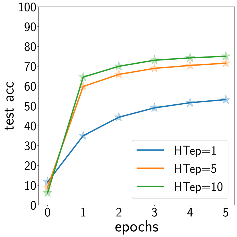
(a) training accuracy

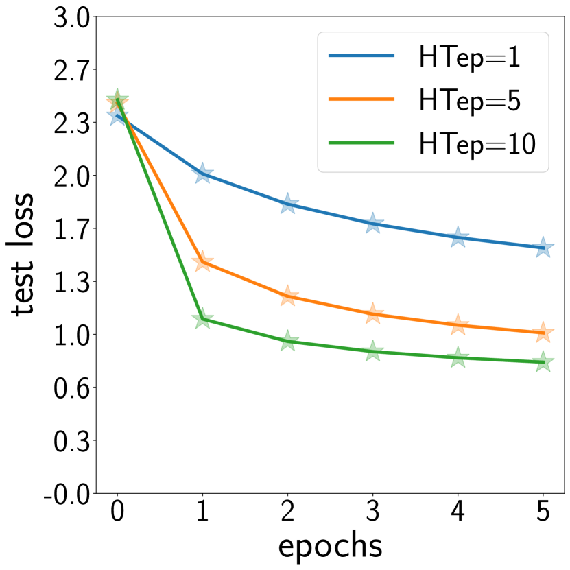
(b) training loss

Figure 5: Format-trained training accuracy as a function of epoch number for a unformatted-trainednetwork trained for 1, 5, and 10 epochs. “HTep” denotes the number of epochs that the unformatted-trainednetwork used. Unformatted training to convergence provides better format-training performance in this experiment.

4.3 Network Capacity and Scale

Fig. 6(a) shows the effect of different widths in the unformatted-trained network followed by a format-trained step. The differences in the width of the unformatted-trained networks are reflected in the different training accuracy in the format-training stage.

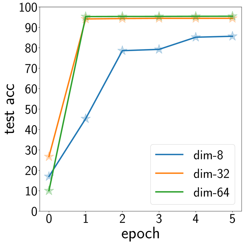
(a)

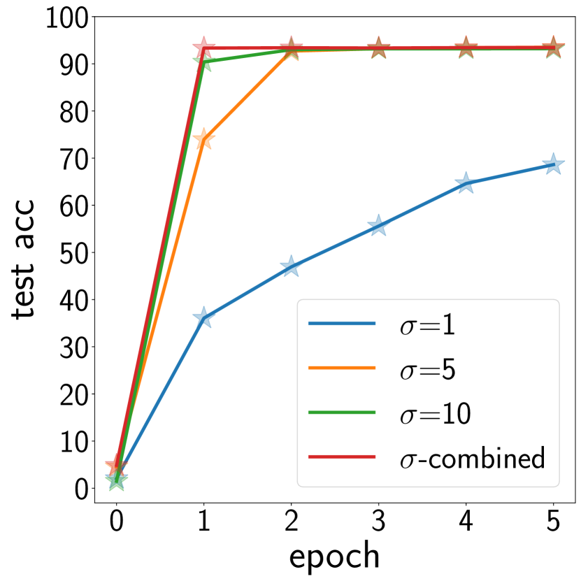
(b)

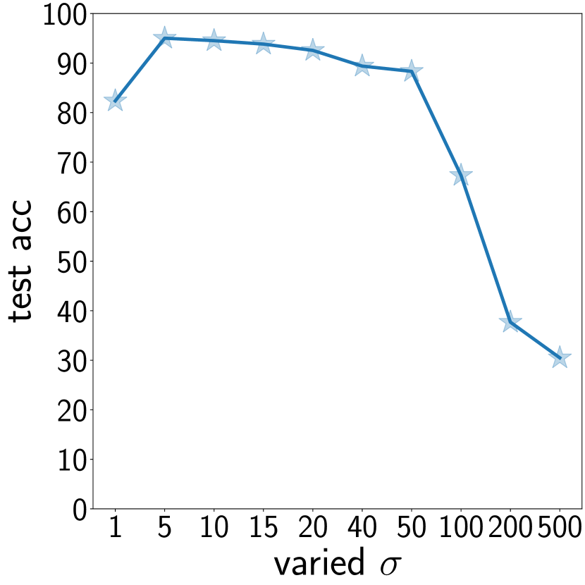
(c)

Figure 6: Test accuracy versus epoch number for differently sized unformatted-trained networks (Fig. 6(a)) and a multiple-scale network  (Fig. 6(b)). The format-training experiment suggests that larger capacity provides more relevant information to the format-training stage. The multiple-scale network labelled with "$\sigma$-combined" demonstrates that using several distinct $\sigma$ values improves performance. Fig. 6(c) gives the test accuracy as a function of $\sigma$ for the network trained with one epoch.

Fig. 6(a) indicates that larger networks (say width-64 compared to width-8) lead to a faster-converging format-training stage. This suggests the HSIC bottleneck objective (6) works effectively on large networks that provide more relevant information to the format-training stage.

As mentioned in previous section, the HSIC results do depend on the chosen $\sigma$. In the multiple-scale network experiment (Fig. 6(b)), we aggregate several unformatted-trained networks with different $\sigma$ together in parallel to better capture dependencies at multiple scales. Our experiment setup trains three parallel HSIC networks having the same five-layered configuration but with different kernel widths $\sigma=1$, $\sigma=5$, and $\sigma=10$. The resulting format-training performance is shown in Fig. 6(b).

The results show format-training on the multiple-scale network outperforms other experiments, suggesting that it is providing additional information relating to the corresponding scale to the format-training stage. It also indicates that a single $\sigma$ is not sufficient to capture all dependencies in these networks. Treating $\sigma$ as a learnable parameter is left for future work.

4.4 Experiments on ResNet

Our previous results aimed at demonstrating the training efficacy of the new paradigm are based on basic fully connected feedforward networks. To show that the paradigm is potentially effective for other architectures, we train a ResNet with the unformatted-trained framework by adding the loss (6) to the output of each residual block.

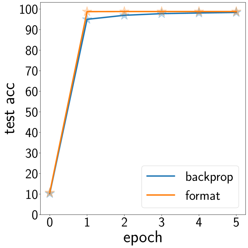
(a) MNIST

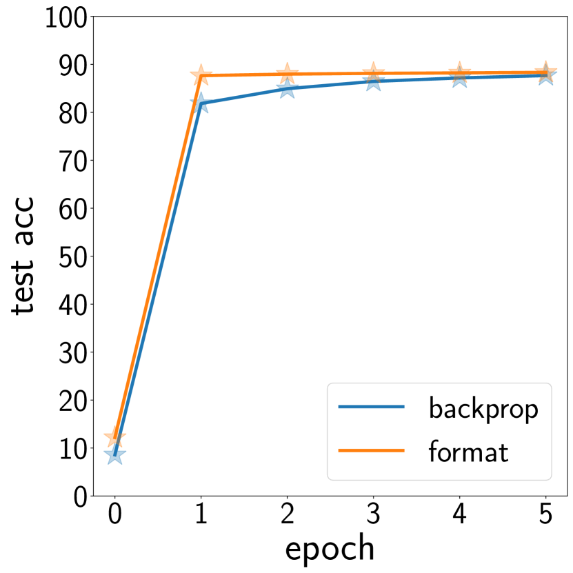
(b) Fashion MNIST

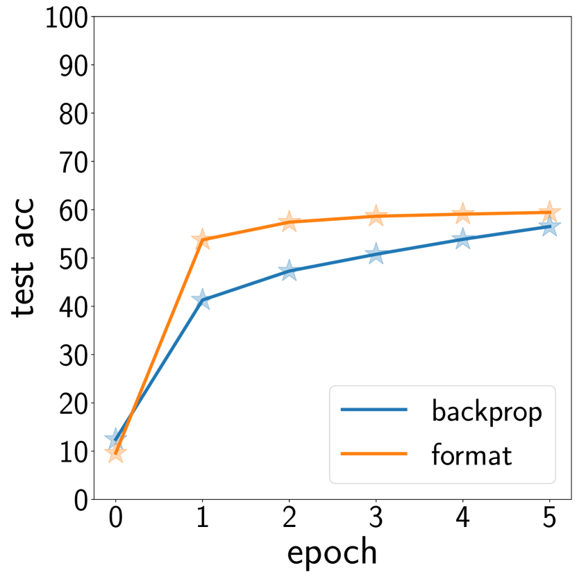
(c) CIFAR10

Figure 7: Test accuracy versus epoch number for ResNet. The performance is shown for the comparison between the ResNet trained with format-training and a backpropagation network.

In Fig. 7, we show the test performance for a network with five convolutional residual blocks on several datasets in the initial epochs. Each experiment includes five unformatted-trained epochs followed by format-training with a one-layer classifier network, and is compared with its standard backpropagation-trained counterpart.

Our results show that the format-training converges more rapidly to high accuracy performance by making use of the distinct representations from the unformatted-trained network. The final test accuracy from Fig. 7 is (98.8%, 88.3%, 59.4%) for format-trained and (98.4%, 87.6%, 56.5%) for backpropagation-trained networks, for MNIST, FashionMNIST, and CIFAR10 respectively. The CIFAR10 result is well below state-of-the-art performance, because we are not using a state-of-the-art architecture. Nevertheless, the HSIC-bottleneck network provides a significant boost in convergence.

5 Conclusion

We present a new approach to train deep neural networks without the use of backpropagation. The method is inspired by the information bottleneck and can be seen as an approximation there-of, but (to our knowledge) is the first approach that sidesteps the well known issues in computing mutual information in deep neural networks by using HSIC as a surrogate. “Unformatted” HSIC-bottleneck training of several standard classification problems results in one-hot output that can be directly permuted to perform classification, with accuracy approximately comparable to that of standard backpropagation training of the same architectures. Performance is further improved by using the outputs as representations for a format-training stage, in which a single layer (and softmax) is appended and trained with conventional SGD, but without backpropagation. The HSIC bottleneck trained network provides good hidden representations by removing irrelevant information and retaining information that is important for the task at hand.

HSIC bottleneck training has several benefits over conventional backpropagation:

• it is able to train deep networks for which backpropagation training fails (Fig. 4);

• it mitigates the vanishing and exploding gradient issues found in conventional backpropagation, since it solves the problem layer-by-layer without the use of the chain rule;

• it removes the need for backward sweeps;

• it potentially allows layers to be trained in parallel, using layerwise block coordinate descent;

• although our approach is not intended to be biologically plausible, it does address the weight transport (?) and update locking problems.

Our work is an initial exploration of backpropagation-free learning using the HSIC bottleneck, and, in common with other explorations of new training methods for deep learning, e.g., (?; ?)) does not attempt to achieve state-of-the-art performance. Future work could consider careful tuning of the $\sigma$ in HSIC to improve performance and evaluate the HSIC-bottleneck approach on different tasks such as regression and generative models.

The HSIC Bottleneck: Supplementary Material
  
  

Relating HSIC to Entropy

Although HSIC is a measure of (in)dependence, its exact relation to mutual information has not been established. Mutual information is defined in terms of entropy, and it has been observed that entropy and Fisher information are related as volume and surface area (?).

In this section we outline an informal argument that HSIC is analogously related to diameter, making use of the identity $I(X,X)=H(X)$. The relation of entropy to volume is easily suggested in the case of a multivariate Gaussian RV with covariance matrix $\mathbf{C}$. The entropy in this case is

$$H(X_{\text{gaussian}}) =\frac{1}{2}\log\left((2\pi e)^{d}|\mathbf{C}|\right)$$

$$\propto\log\det\mathbf{C}\quad+\quad\text{constant}$$

Here the interpretation as a “volume” can be seen through the presence of the determinant. For comparison with HSIC (below), note that $\mathbf{C}$ is symmetric and can be diagonalized with real eigenvalues,

$$\det\mathbf{C}=\det\mathbf{U}\bm{\Lambda}\mathbf{U}^{T}=\det\bm{\Lambda}=\prod\lambda_{k}$$

Turning to HSIC, denoting $\tilde{\mathbf{K}}_{X}=\mathbf{H}\mathbf{K}_{X}\mathbf{H}$ (and similarly for $\mathbf{Y}$, the HSIC computation is $\frac{1}{n^{2}}\operatorname{tr}\tilde{\mathbf{K}}_{X}\tilde{\mathbf{K}}_{Y}$. HSIC(X,X) is thus simply $\frac{1}{n^{2}}\operatorname{tr}\tilde{\mathbf{K}}_{X}^{2}$, i.e. the (scaled) squared Frobenious norm of the feature covariance matrix.

Now in general $\|\mathbf{A}\|_{F}^{2}=\sum\lambda_{k}^{2}$ because

$$\operatorname{tr}\mathbf{A}^{T}\mathbf{A}=\operatorname{tr}(\mathbf{P}\bm{\Lambda}\mathbf{P}^{-1})(\mathbf{P}\bm{\Lambda}\mathbf{P}^{-1})=\operatorname{tr}\mathbf{P}\bm{\Lambda}^{2}\mathbf{P}^{-1}=\operatorname{tr}\bm{\Lambda}^{2}$$

making use of the Jordan normal decomposition (or eigendecomposition in our case because $\tilde{\mathbf{K}}_{X}$ is symmetric).

In summary, entropy is related to volume, as can be see in the Gaussian case through the presence of the determinant, i.e. the product of the eigenvalues. HSIC(X,X) is related to the Frobenius norm, which is a sum of eigenvalues, i.e. a “diameter”.

Toy unformatted-training solve

Fig. 3 has shown that unformatted-training discriminates class signals during the training, resulting a one-hot effect. We did a further experiment based on a simple model sized 784-256-128-64-32-16-8-1 with backpropagation and unformatted-training. As is convention, we appended an output layer $O\in\mathbb{R}^{10}$ to the backpropagation model to support the cross-entropy objective. The goal of this experiment is to see how well the unformatted-training can separate the signal classes in $\mathbb{R}^{1}$. Although the results change based on the random seed, we found that unformatted-training usually produces better separation than backpropagation (Fig. 8).

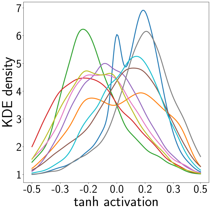
(a) Backpropagation

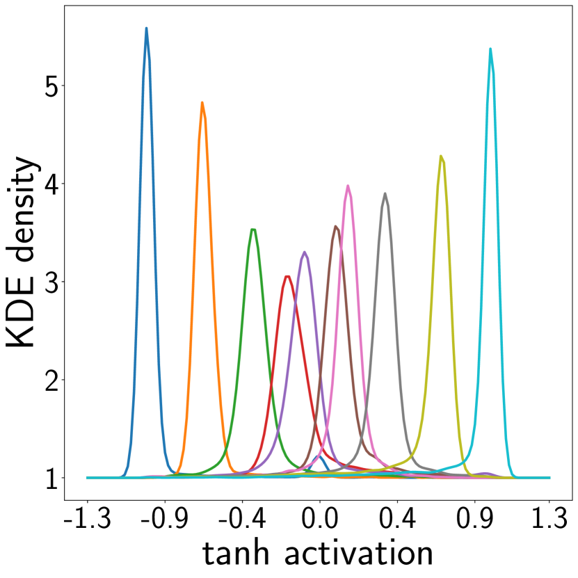
(b) Unformatted training

Figure 8: The tanh classed activation in $\mathbb{R}^{1}$ distribution of MNIST between backpropagation Fig 8(a), and unformatted-training Fig 8(b). Each curve represents the activation distribution from particular image category. The distribution is generated by Gaussian Kernel Density Estimation (KDE).

Differences in Arxiv version 2

All the experimental results are new and generally show the test performance over additional epochs. The figures are improved to be more legible. The experiment hyperparameters benefit from a modest hyperparameter search, whereas the hyperparameters in the first draft were manually chosen and did not reflect the best performance of either our method or the baseline. The text has been clarified to emphasize that we do not claim biological plausibiltiy; rather, our method merely shares characteristics (no backpropagation, weight transport, or update locking) with other recent methods that are regarded as making some progress toward this goal.

References

- [Alemi et al. 2017] Alemi, A. A.; Fischer, I.; Dillon, J. V.; and Murphy, K. 2017. Deep variational information bottleneck. In ICLR. OpenReview.net.
- [Amjad and Geiger 2018] Amjad, R. A., and Geiger, B. C. 2018. How (not) to train your neural network using the information bottleneck principle. CoRR abs/1802.09766.
- [Baddeley, Foldiak, and Hancock 1999] Baddeley, R.; Foldiak, P.; and Hancock, P., eds. 1999. Information Theory and the Brain. Cambridge University Press.
- [Balduzzi, Vanchinathan, and Buhmann 2015] Balduzzi, D.; Vanchinathan, H.; and Buhmann, J. 2015. Kickback cuts backprop’s red-tape: Biologically plausible credit assignment in neural networks. In Proc. AAAI.
- [Banerjee and Montúfar 2018] Banerjee, P. K., and Montúfar, G. 2018. The variational deficiency bottleneck. CoRR abs/1810.11677.
- [Belghazi et al. 2018] Belghazi, I.; Rajeswar, S.; Baratin, A.; Hjelm, R. D.; and Courville, A. C. 2018. MINE: mutual information neural estimation. CoRR abs/1801.04062.
- [Blaschko and Gretton 2008] Blaschko, M. B., and Gretton, A. 2008. A Hilbert-Schmidt dependence maximization approach to unsupervised structure discovery. In Proc. 6th Int. Workshop on Mining and Learning with Graphs.
- [Brakel and Bengio 2018] Brakel, P., and Bengio, Y. 2018. Learning independent features with adversarial nets for non-linear ICA. https://openreview.net.
- [Choromanska et al. 2019] Choromanska, A.; Cowen, B.; Kumaravel, S.; Luss, R.; Rigotti, M.; Rish, I.; Diachille, P.; Gurev, V.; Kingsbury, B.; Tejwani, R.; and Bouneffouf, D. 2019. Beyond backprop: Online alternating minimization with auxiliary variables. In ICML, 1193–1202.
- [Cover and Thomas 2006] Cover, T. M., and Thomas, J. A. 2006. Elements of Information Theory. New York, NY, USA: Wiley-Interscience.
- [de Souza Farias and Maziero 2018] de Souza Farias, T., and Maziero, J. 2018. Gradient target propagation. CoRR abs/1810.09284.
- [Fukumizu et al. 2008] Fukumizu, K.; Gretton, A.; Sun, X.; and Schölkopf, B. 2008. Kernel measures of conditional dependence. In Platt, J. C.; Koller, D.; Singer, Y.; and Roweis, S. T., eds., NIPS. 489–496.
- [Goldfeld et al. 2018] Goldfeld, Z.; van den Berg, E.; Greenewald, K. H.; Melnyk, I.; Nguyen, N.; Kingsbury, B.; and Polyanskiy, Y. 2018. Estimating information flow in neural networks. CoRR abs/1810.05728.
- [Gretton et al. 2005] Gretton, A.; Bousquet, O.; Smola, A.; and Schölkopf, B. 2005. Measuring statistical dependence with Hilbert-Schmidt norms. In Proc. Int. Conf. Algorithmic Learning Theory, 63–77. Springer-Verlag.
- [Ioffe and Szegedy 2015] Ioffe, S., and Szegedy, C. 2015. Batch normalization: Accelerating deep network training by reducing internal covariate shift. CoRR abs/1502.03167.
- [Kohan, Rietman, and Siegelmann 2018] Kohan, A. A.; Rietman, E. A.; and Siegelmann, H. T. 2018. Error forward-propagation: Reusing feedforward connections to propagate errors in deep learning. CoRR abs/1808.03357.
- [Kolchinsky, Tracey, and Wolpert 2017] Kolchinsky, A.; Tracey, B. D.; and Wolpert, D. H. 2017. Nonlinear information bottleneck. CoRR abs/1705.02436.
- [Kwak and Chong-Ho Choi 2002] Kwak, N., and Chong-Ho Choi. 2002. Input feature selection by mutual information based on Parzen window. IEEE Tran. Pattern Analysis and Machine Intelligence 24(12):1667–1671.
- [Lillicrap et al. 2016] Lillicrap, T. P.; Cownden, D.; Tweed, D. B.; and Akerman, C. J. 2016. Random synaptic feedback weights support error backpropagation for deep learning. Nature Communications 7.
- [Lopez et al. 2018] Lopez, R.; Regier, J.; Yosef, N.; and Jordan, M. I. 2018. Information constraints on auto-encoding variational bayes. CoRR abs/1805.08672.
- [Moskovitz, Litwin-Kumar, and Abbott 2018] Moskovitz, T. H.; Litwin-Kumar, A.; and Abbott, L. F. 2018. Feedback alignment in deep convolutional networks. CoRR abs/1812.06488.
- [Saxe et al. 2018] Saxe, A. M.; Bansal, Y.; Dapello, J.; Advani, M.; Kolchinsky, A.; Tracey, B. D.; and Cox, D. D. 2018. On the information bottleneck theory of deep learning. In International Conference on Learning Representations.
- [Sejdinovic et al. 2012] Sejdinovic, D.; Gretton, A.; Sriperumbudur, B. K.; and Fukumizu, K. 2012. Hypothesis testing using pairwise distances and associated kernels (with appendix). CoRR abs/1205.0411.
- [Shwartz-Ziv and Tishby 2017] Shwartz-Ziv, R., and Tishby, N. 2017. Opening the black box of deep neural networks via information. CoRR abs/1703.00810.
- [Sriperumbudur, Fukumizu, and Lanckriet 2010] Sriperumbudur, B. K.; Fukumizu, K.; and Lanckriet, G. 2010. On the relation between universality, characteristic kernels and RKHS embedding of measures. In International Conference on Artificial Intelligence and Statistics, 773–780.
- [Sugiyama and Yamada 2012] Sugiyama, M., and Yamada, M. 2012. On kernel parameter selection in Hilbert-Schmidt independence criterion. IEICE Transactions on Information and Systems E95D.
- [Tishby, Pereira, and Bialek 1999] Tishby, N.; Pereira, F. C.; and Bialek, W. 1999. The information bottleneck method. In Allerton Conference on Communication, Control, and Computing.
- [Tschannen et al. 2019] Tschannen, M.; Djolonga, J.; Rubenstein, P. K.; Gelly, S.; and Lucic, M. 2019. On mutual information maximization for representation learning. CoRR abs/1907.13625.
- [Vepakomma et al. 2019] Vepakomma, P.; Gupta, O.; Dubey, A.; and Raskar, R. 2019. Reducing leakage in distributed deep learning for sensitive health data. In ICLR AI for social good workshop.
- [Werbos 1990] Werbos, P. J. 1990. Backpropagation through time: what it does and how to do it. Proceedings of the IEEE 78(10):1550–1560.
- [Wu et al. 2018] Wu, D.; Zhao, Y.; Tsai, Y.-H. H.; Yamada, M.; and Salakhutdinov, R. 2018. "Dependency Bottleneck" in auto-encoding architectures: an empirical study. CoRR abs/1802.05408.