Repair Pipelining for Erasure-Coded Storage: Algorithms and Evaluation

Abstract

We propose repair pipelining, a technique that speeds up the repair performance in general erasure-coded storage. By carefully scheduling the repair of failed data in small-size units across storage nodes in a pipelined manner, repair pipelining reduces the single-block repair time to approximately the same as the normal read time for a single block in homogeneous environments. We further design different extensions of repair pipelining algorithms for heterogeneous environments and multi-block repair operations. We implement a repair pipelining prototype, called ECPipe, and integrate it as a middleware system into two versions of Hadoop Distributed File System (HDFS) (namely HDFS-RAID and HDFS-3) as well as Quantcast File System (QFS). Experiments on a local testbed and Amazon EC2 show that repair pipelining significantly improves the performance of degraded reads and full-node recovery over existing repair techniques.

1 Introduction

Distributed storage systems rely on data redundancy to provide fault tolerance, so as to maintain availability and durability. Replication, which is traditionally used by production systems [11, 18], provides the simplest form of redundancy by keeping identical copies of data in different storage nodes. However, the raw storage cost of replication is overwhelming, especially with the massive scale of data we face today. Erasure coding provides a low-cost redundancy alternative that incurs significantly lower storage overhead than replication at the same fault tolerance level [52]. Today’s distributed storage systems adopt erasure coding to protect data against failures in clustered [17, 23, 41] or geo-distributed environments [6, 44, 32, 12], and reportedly save petabytes of storage [23, 32]. In a nutshell, erasure coding takes two configurable parameters $n$ and $k$ (where $k<n$) as input. It transforms $k$ fixed-size units (called blocks) of original data into a set of $n$ coded blocks of the same size, such that any $k$ out of $n$ (coded) blocks can reconstruct all original data; in other words, the original data remains available even if any $n-k$ blocks are failed (either lost or unavailable). For example, if $n=14$ and $k=10$ (the same parameters used in Facebook’s erasure coding deployment [32]), the storage overhead is only $1.4\times$, while tolerating $n-k=4$ failed blocks. In contrast, replication incurs $5\times$ storage overhead to tolerate the same number of failed blocks. We elaborate erasure coding in detail in §2.1.

Although achieving storage efficiency, erasure coding has a drawback of incurring high repair penalty. Specifically, in erasure-coded storage, the repair of a single failed block needs to read multiple available blocks for reconstruction; in other words, it reads more available data than the size of a failed block. This is in contrast to replication, whose repair can be simply done by reading another replica that is of the same size as the failed block. The excessive data not only increases the read time to failed data as opposed to normal reads, but also consumes bandwidth resources that could otherwise be made available for other foreground jobs [41]. Thus, erasure coding in practice is mainly used for storing less frequently read (i.e., warm/cold) data that needs long-term persistence [23, 8, 32], while frequently read (i.e., hot) data remains replicated for efficient access.

To mitigate the repair penalty of erasure coding, prior studies propose new constructions of erasure codes that significantly reduce the amount of repair traffic (e.g., [16, 23, 26, 45, 42, 40, 36, 51]); in particular, the minimum-storage regenerating (MSR) codes [16, 40, 36, 51] provably minimize the amount of repair traffic subject to the minimum storage redundancy. While the repair time is effectively reduced due to the reduction of repair traffic, it remains higher than the normal read time in general since the minimum size of repair traffic remains larger than the size of the failed block. In view of this, we pose the following question: Can we further reduce the repair time of erasure coding to almost the same as the normal read time? This creates opportunities for applying erasure coding to hot data for high storage efficiency, while preserving read performance.

We present a general technique called repair pipelining to speed up the repair performance in general erasure-coded storage. Its main idea is to decompose the repair of a block in small-size units (called slices) and carefully schedule the repair of multiple slices in a pipelined manner (analogous to wormhole routing [33]), so as to distribute the repair traffic and fully utilize the bandwidth resources of storage nodes. Contrary to the conventional wisdom that the repair of erasure coding is a slow operation, repair pipelining reduces the single-block repair time to almost the same as the normal read time for a single available block, regardless of coding parameters, in homogeneous environments where network links have identical bandwidth limits. Also, it provides different heuristics to mitigate the single-block repair time in heterogeneous environments where network links have different bandwidth limits. Furthermore, it supports various practical erasure codes that are adopted by today’s production systems, including the classical Reed-Solomon codes [43] and the recent Local Reconstruction Codes [23].

We point out that the notion of repair pipelining has also been studied in several publications by other researchers (e.g., [24, 53, 9]); note that PUSH [24] was published before the conference version [29] of this paper. PUSH [24] addresses full-node recovery by constructing a linear repair path through $k$ available blocks and performing block-level repair pipelining. For different block sizes (a.k.a. request unit sizes [24]), PUSH achieves $1/k$ of the repair time of conventional repair in full-node recovery. Thus, we do not claim that the concept of repair pipelining is the main contribution of this paper. Instead, our contributions are to demonstrate the viability of repair pipelining in various deployment environments through in-depth analysis and prototype evaluation. As we show in this paper, applying slice-level repair pipelining is non-trivial, since its repair performance gain also depends on how the slice-level repair sub-operations are scheduled. We refer readers to §7 for more detailed comparisons of our work with the related approaches.

To summarize, we make the following contributions.

• We design repair pipelining to address two types of repair operations: degraded reads and full-node recovery. We show that repair pipelining reduces the single-block repair time to almost the same as the normal read time for a single available block in homogeneous environments.

• We extend repair pipelining to address heterogeneous environments and present three extensions of repair pipelining algorithms: the first one allows parallel reads of a repaired block when the bandwidth between the storage system and the node that requests for the repaired block is limited; the second one finds an optimal repair path for hierarchical data centers in which the cross-rack link bandwidth is limited; the third one finds an optimal repair path across storage nodes such that the repair time is minimized in a heterogeneous environment where network links have arbitrary bandwidth limits.

• We further extend repair pipelining for repairing multiple failed blocks within the set of $n$ coded blocks. We show that it reduces the multi-block repair time to almost the same as the total normal read time for $f$ available blocks in homogeneous environments, where $f$ is the number of failed blocks being repaired.

• We implement a repair pipelining prototype called ECPipe, which runs as a middleware system atop an existing storage system and performs repair operations on behalf of the storage system. As a proof of concept, we integrate ECPipe into two versions of Hadoop Distributed File System (HDFS) [49], namely HDFS-RAID [1] and Hadoop 3.1.1 HDFS (HDFS-3) [2], as well as Quantcast File System (QFS) [35]. All the integrations only make minor changes (with no more than 245 lines of code) to the code base of each storage system. The latest source code of our ECPipe prototype is available at: http://adslab.cse.cuhk.edu.hk/software/ecpipe.

• We evaluate repair pipelining on a local cluster and two geo-distributed Amazon EC2 clusters (one in North America and one in Asia). We compare it with two existing repair approaches in which the single-block repair time increases with $k$ (recall that $k$ is the number of blocks of original data for encoding): (i) conventional repair that is used by classical Reed-Solomon codes [43] and achieves $O(k)$ single-block repair time, and (ii) the recently proposed partial-parallel-repair (PPR) scheme [31], which achieves $O(\log_{2}k)$ single-block repair time by parallelizing partial repair operations in a hierarchical manner. In contrast, repair pipelining achieves $O(1)$ single-block repair time if there is a sufficiently large number of slices per block (i.e., independent of $k$). Our experiments show that repair pipelining reduces the single-block repair time by nearly 90% and 70% compared to conventional repair and PPR, respectively. It also reduces the multi-block repair time by around 60% compared to conventional repair, as well as improves the repair performance in HDFS-RAID, HDFS-3, and QFS deployments. Furthermore, we show that our current repair pipelining implementation in ECPipe, by carefully parallelizing slice-level repair sub-operations, achieves the highest performance for large block sizes compared to several baseline repair pipelining implementations (§6.4).

The rest of the paper proceeds as follows. In §2, we describe the basics of erasure coding and motivate the repair problem. In §3, we present the design of repair pipelining. In §4, we extend repair pipelining for heterogeneous environments and multi-block repair operations. In §5, we present implementation details of ECPipe and show how it is integrated into existing open-source distributed storage systems. In §6, we present evaluation results. In §7, we review related work, and finally, in §8, we conclude the paper.

2 Background and Motivation

We first present the basics of erasure coding and explain the repair problem. We then motivate the need of minimizing the repair time in erasure-coded storage.

2.1 Basics

We consider a distributed storage system (e.g., GFS [18], HDFS [49], and Azure [11]) that manages large-scale datasets and stores files as fixed-size blocks, which form the basic read/write units. The block size is often large, ranging from 64 MiB [18] to 256 MiB [42], to mitigate I/O seek overhead. Erasure coding is applied to a collection of blocks. Specifically, an erasure code is typically configured with two integer parameters $(n,k)$, where $k<n$. An $(n,k)$ code divides blocks into groups of $k$. For every $k$ (uncoded) blocks, it encodes them to form $n$ coded blocks, such that any $k$ out of $n$ coded blocks can be decoded to the original $k$ uncoded blocks. The set of $n$ coded blocks is called a stripe. A large-scale storage system stores data of multiple stripes, all of which are independently encoded. The $n$ coded blocks of each stripe are distributed across $n$ distinct nodes to tolerate any $n-k$ node failures. Most practical erasure codes are systematic, such that $k$ of $n$ coded blocks are identical to the original uncoded blocks and hence can be directly accessed without decoding. Nevertheless, our design treats both uncoded and coded blocks the same, so we simply refer to them as “blocks”.

Many erasure code constructions have been proposed in the literature (see survey [37] and §7). Among all erasure codes, Reed-Solomon (RS) codes [43] are the most popular erasure codes that are widely deployed in production [17, 41, 35]. There are two key properties of RS codes: (i) maximum distance separable (MDS), meaning that RS codes can reconstruct the original $k$ uncoded blocks from any $k$ out of $n$ coded blocks with the minimum storage redundancy (i.e., $n/k$ times the original data size), and (ii) general, meaning that RS codes support any $n$ and $k$ (provided that $k<n$).

Practical erasure codes (e.g., RS codes) often satisfy linearity. Specifically, for each stripe of an $(n,k)$ code, let $\{B_{1},B_{2},\cdots,B_{k}\}$ denote any $k$ blocks of a stripe. Any block in the same stripe, say $B^{*}$, can be computed from a linear combination of the $k$ blocks as $B^{*}=\sum_{i=1}^{k}a_{i}B_{i}$, where $a_{i}$’s ($1\leq i\leq k$) are decoding coefficients specified by a given erasure code. All additions and multiplications are based on Galois Field arithmetic over $w$-bit units called words; in particular, an addition is equivalent to bitwise XOR. Note that the additions of $a_{i}B_{i}$’s are associative (i.e., the additions can be in any order). Some constraints may be applied; for example, RS codes require $n\leq 2^{w}+1$ [38]. Each block is partitioned into multiple $w$-bit words, such that the words at the same offset of each block of a stripe are encoded together, as shown in Figure 1.

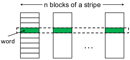
Figure 1: In erasure coding, blocks are partitioned into words, such that words at the same offset of each block of a stripe are encoded together.

2.2 Repair

In this paper, we focus on two types of repair operations in erasure-coded storage: (i) degraded reads to temporarily unavailable blocks (e.g., due to power outages, network disconnection, system maintenance, etc.) or lost blocks that are yet recovered; and (ii) full-node recovery for restoring all lost blocks of a failed node (e.g., due to disk crashes, sector errors, etc.). Each failed block (either lost or unavailable) is reconstructed in a destination termed requestor, which can be a new node that replaces a failed node, or a client that issues degraded reads. Note that there may be one or multiple requestors when multiple failed blocks are reconstructed.

Erasure coding triggers more repair traffic than the size of failed data to be reconstructed. For example, for $(n,k)$ RS codes, repairing a failed block reads $k$ available blocks of the same stripe from other nodes (i.e., $k$ times the block size). Some repair-friendly erasure codes (e.g., [16, 26, 23, 45, 42, 40, 36, 51]) are designed to reduce the repair traffic (see details in §7), but the amount of repair traffic per block remains larger than the size of a block. In distributed storage systems, network bandwidth is often the most dominant factor in the repair performance as extensively shown by previous work [16, 50, 31] (see further justifications in §2.3). Thus, the amplification of repair traffic implies the congestion at the downlink of the requestor, thereby increasing the overall repair time.

To understand the repair penalty of erasure coding, we use RS codes as an example and call this repair approach conventional repair. Suppose that a requestor $R$ wants to repair a failed block $B^{*}$. It can be done by reading $k$ available blocks from any $k$ working nodes, called helpers. Without loss of generality, let $R$ contact $k$ helper nodes $N_{1}$, $N_{2}$, $\cdots$, $N_{k}$, which store available blocks $B_{1}$, $B_{2}$, $\cdots$, $B_{k}$, respectively. To make our discussion clear, we divide the repair process into timeslots, such that only one block can be transmitted across a network link in each timeslot. Figure 2(a) shows how conventional repair works for $k=4$. Since $R$ needs to retrieve the $k$ blocks $B_{1}$, $B_{2}$, $\cdots$, $B_{k}$, all $k$ transmissions must traverse the downlink of $R$. Overall, the repair in Figure 2(a) takes four timeslots. In general, conventional repair needs $k$ timeslots to repair a failed block.

Conventional repair can address the repair of multiple concurrently failed blocks in the same stripe. Suppose that there are $f\leq n-k$ failed blocks in a stripe (i.e., fault tolerance is still maintained). Our goal is to repair the $f$ failed blocks in $f$ requestors, each of which stores a reconstructed block. The multi-block repair can be done by dedicating one of the $f$ requestors to retrieve $k$ available blocks from $k$ helper nodes. Since the dedicated requestor has sufficient information to reconstruct all original uncoded data, it can also reconstruct all $f$ failed blocks. Thus, it can locally store one of the reconstructed blocks and send the $f-1$ reconstructed blocks to the other $f-1$ requestors. The number of timeslots for a multi-block repair is $k+f-1$ timeslots.

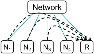
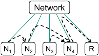
(a) Conventional repair	(b) PPR

Figure 2: Examples of conventional repair and PPR in a single-block repair.

A drawback of conventional repair is that the bandwidth usage distribution is highly skewed: the downlink of the requestor is highly congested, while the links among helpers are not fully utilized. PPR [31] builds on the linearity and addition associativity of erasure coding by decomposing a repair operation into multiple partial operations that are distributed across all helpers. This distributes bandwidth usage across the links of helpers. Figure 2(b) shows how PPR repairs $B^{*}$ for $k=4$. In the first timeslot, $N_{2}$ and $N_{4}$ receive blocks $a_{1}B_{1}$ and $a_{3}B_{3}$ from $N_{1}$ and $N_{3}$, respectively. Since the transmissions use different links, they can be done simultaneously in a single timeslot. In the second timeslot, $N_{2}$ combines the received $a_{1}B_{1}$ and its locally stored block $B_{2}$ to obtain $a_{1}B_{1}+a_{2}B_{2}$ and sends it to $N_{4}$. In the third timeslot, $N_{4}$ combines all received blocks and its own block $B_{4}$ to obtain $a_{1}B_{1}+a_{2}B_{2}+a_{3}B_{3}+a_{4}B_{4}$, and sends it to $R$. This hierarchical approach reduces the overall single-block repair time to only three timeslots. In general, PPR needs $\lceil\log_{2}(k+1)\rceil$ timeslots to repair a failed block. Note that how to generalize PPR for repairing multiple failed blocks in a stripe is still an unexplored issue.

2.3 Motivation

Although PPR reduces the single-block repair time, the bandwidth usage distribution remains not fully balanced; for example, the downlink of $N_{4}$ in Figure 2(b) still carries more repair traffic than other links. Thus, the repair time is still bottlenecked by the link with the most repair traffic. This motivates us to design a new repair scheme that can more efficiently utilize bandwidth resources, with the primary goal of minimizing the repair time.

Minimizing the repair time is critical to both availability and durability. In terms of availability, field studies show that transient failures (i.e., no data loss) account for over 90% of failure events [17]. Thus, most repairs are expected to be degraded reads rather than full-node recovery. Since degraded reads are issued when clients request unavailable data, achieving fast degraded reads not only improves availability but is also critical for meeting customer service-level agreements [23]. In terms of durability, minimizing the repair time also minimizes the window of vulnerability. By recovering any failed block in a timely manner, we maintain the redundancy level for fault-tolerant storage. This avoids any unrecoverable data loss if the number of failed blocks exceeds the tolerable limit (i.e., $n-k$ blocks for an $(n,k)$ code).

Our work targets distributed storage environments in which network bandwidth is the bottleneck. Although modern data centers now scale to high network speeds, they are typically shared by a mix of application workloads. Thus, the network bandwidth available for repair tasks is often throttled [23, 50]. Also, modern data centers often have hierarchical network topologies by organizing nodes in racks, in which the cross-rack link bandwidth is limited (e.g., due to replica writes [13] or compute job traffic [7, 25]). To tolerate rack failures, data centers distribute each stripe across racks [17, 23, 45, 42]. Thus, the repair of any failed block inevitably retrieves available blocks from other racks and triggers cross-rack transmissions. The repair performance will be bottlenecked by the limited cross-rack link bandwidth.

3 Repair Pipelining

We present the design of repair pipelining. We first state our goals and assumptions (§3.1). We then explain how repair pipelining addresses degraded reads (§3.2) and full-node recovery (§3.3).

3.1 Goals and Assumptions

Repair pipelining also exploits the linearity and addition associativity of erasure codes as in PPR [31], yet it parallelizes the repair across helpers in an inherently different way. It focuses on (i) eliminating bottlenecked links (i.e., no link transmits more traffic than others) and (ii) effectively utilizing bandwidth resources during a repair (i.e., links should not be idle for most times), so as to ultimately minimize the single-block repair time to the normal read time for a single block in homogeneous environments where all links have the same bandwidth.

Repair pipelining is mainly designed for speeding up the repair of a single failed block per stripe, which is much more common than the repair of multiple failed blocks per stripe in practice [23, 41] (e.g., over 98% of repair cases are single-block repair operations). Optimizing a single-block repair is also the main design goal of most existing repair-friendly erasure codes that aim to minimize the amount of repair traffic [16, 26, 23, 45, 42, 40, 36, 51]. In this section, we focus on studying the single-block repair for one stripe and multiple stripes. The former occurs when a requestor issues a degraded read to an unavailable block; the latter occurs when all lost data of a single failed node is recovered in one or multiple requestors in full-node recovery.

If a stripe has multiple failed blocks, we can also extend repair pipelining to trigger a multi-block repair, which we show incurs less repair time than conventional repair (§2.2). See §4.4 for details.

Repair pipelining does not design new repair-friendly erasure codes that minimize the repair traffic (the same assumption is made in PPR [31]). Instead, each repair of a single failed block still reads $k$ available blocks as in conventional repair, yet it spreads the repair traffic across all $k$ helpers so as to fully utilize bandwidth resources. The failed block can then be reconstructed as a linear combination of the $k$ available blocks.

Some repair-friendly codes, including locally repairable codes [23, 45] and Rotated RS codes [26], work by reconstructing a failed block through a linear combination of fewer than $k$ available blocks. In this case, we can also combine repair pipelining with such repair-friendly codes to reduce the single-block repair time while preserving their repair traffic savings. We evaluate such a combination in §6.1. An interesting open question is to augment repair pipelining with the optimal repair of general repair-friendly codes (e.g., regenerating codes [16]), so as to simultaneously reduce the single-block repair time and minimize the repair traffic. We pose this question as a future work.

3.2 Degraded Reads

We first study how repair pipelining reconstructs a single block of a stripe in a requestor in a degraded read. We start with a naïve approach. Specifically, we arrange $k$ helpers and the requestor as a linear path, i.e., $N_{1}\rightarrow N_{2}\rightarrow\cdots\rightarrow N_{k}\rightarrow R$. At a high level, to repair a failed block $B^{*}$, $N_{1}$ sends $a_{1}B_{1}$ to $N_{2}$. Then $N_{2}$ combines $a_{1}B_{1}$ with its own block $B_{2}$ and sends $a_{1}B_{1}+a_{2}B_{2}$ to $N_{3}$. The process repeats, and finally, $N_{k}$ sends $R$ the combined result, which is $B^{*}$. The whole repair incurs $k$ transmissions that span across $k$ different links. Thus, there is no bottlenecked link. However, this naïve approach underutilizes bandwidth resources, since there is only one block-level transmission in each timeslot. The whole repair still takes $k$ timeslots, same as in conventional repair (§2.2).

Thus, repair pipelining decomposes the repair of a block into the repair of a set of $s$ small fixed-size units called slices $S_{1},S_{2},\cdots,S_{s}$. It also partitions each block $B_{i}$ ($1\leq i\leq k$) into $s$ slices $B_{i,1},B_{i,2},\cdots,B_{i,s}$. It pipelines the repair of each slice through the linear path. To repair the first slice $S_{1}$, $N_{1}$ sends $a_{1}B_{1,1}$ to $N_{2}$, $N_{2}$ sends $a_{1}B_{1,1}+a_{2}B_{2,1}$ to $N_{3}$, and so on. Note that when $N_{2}$ sends the slice $a_{1}B_{1,1}+a_{2}B_{2,1}$ to $N_{3}$, $N_{1}$ can start the repair of the second slice $S_{2}$ by sending $a_{1}B_{1,2}$ to $N_{2}$ without interfering in the transmission from $N_{2}$ to $N_{3}$. Thus, we can parallelize the slice-level transmissions. Each slice-level transmission over a link only takes $\frac{1}{s}$ timeslots. Figure 3 shows how repair pipelining works for $k=4$ and $s=6$.

A slice can have an arbitrarily small size, provided that Galois Field arithmetic can be performed (§2.1). For RS codes, the minimum size of a slice is a $w$-bit word; if $w=8$, a word denotes a byte. On the other hand, practical distributed storage systems store data in large-size blocks, typically 64 MiB or even larger (§2.1). Since a coding unit (i.e., word) has a much smaller size than a read/write unit (i.e., block), we can parallelize a block-level repair operation into more fine-grained slice-level repair sub-operations. Having smaller-size slices improves parallelism, yet it increases the overhead of issuing many requests for transmitting slices over the network. We study the impact of the slice size in §6.

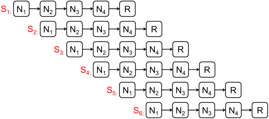
Figure 3: Repair pipelining with $k=4$ and $s=6$.

We analyze the time complexity of repair pipelining. Here, we neglect the overheads due to computation and disk I/O, which we assume cost less time than network transmission; in fact, both computation and disk I/O operations can also be executed in parallel with network transmission in actual implementation (§5). Each slice-level transmission over a link takes $\frac{1}{s}$ timeslots. The repair of each slice takes $\frac{k}{s}$ timeslots to traverse the linear path, and $N_{1}$ starts to transmit the last slice after $\frac{s-1}{s}$ timeslots. Thus, the whole repair time, which is given by the total number of timeslots to transmit all slices through the linear path, is $\frac{s-1+k}{s}=1+\frac{k-1}{s}$ timeslots. In practice, $k$ is of moderate size to avoid large coding overhead [38] (e.g., $k=12$ in Azure [23] and $k=10$ in Facebook [41]), while $s$ can be much larger (e.g., $s=$ 2,048 for 32 KiB slices in a 64 MiB block). Thus, we have $1+\frac{k-1}{s}\to 1$, as $s$ is sufficiently large.

Repair pipelining connects multiple helpers as a linear path, so its repair performance is bottlenecked by the presence of poorly performed links/helpers (i.e., stragglers). We emphasize that any repair scheme of erasure coding faces the similar problem, as it retrieves available data from multiple helpers for data reconstruction; for example, conventional repair for $(n,k)$ MDS codes needs to retrieve the available data from $k$ helpers. We address the straggler problem by taking into account heterogeneity and bypassing stragglers via helper selection (§4.3). Also, if any helper fails during an ongoing repair, the progress of repair pipelining will be stalled. In this case, we restart the whole repair process with a new set of available helpers and trigger a multi-block repair (§4.4).

3.3 Full-Node Recovery

We now study how repair pipelining addresses a multi-stripe repair (one failed block per stripe) when recovering a full-node failure. As the stripes are independently encoded, we can parallelize the multiple single-stripe repair operations. However, since each repair involves a number of helpers, if one helper is chosen in many repair operations of different stripes, it will become overloaded and slow down the overall repair performance. In practice, each stripe is stored in a different set of storage nodes spanning across the network. Our goal is to distribute the load of a multi-stripe repair across all helpers as evenly as possible.

We adopt a simple greedy scheduling approach for the selection of helpers. For each node in the storage system, repair pipelining keeps track of a timestamp indicating when the node was last selected as a helper for a single-stripe repair. To repair a failed block of a stripe, we select $k$ out of $n-1$ available helpers in the stripe that have the smallest timestamps; in other words, the $k$ selected helpers are the least recently selected ones in previous requests. Choosing $k$ out of the $n-1$ helpers can be done in $O(n)$ time using the quick select algorithm [19] (based on repeated partitioning of quick sort). We use a centralized coordinator to manage the selection process (§5). Our greedy scheduling emphasizes simplicity in deployment. We can also adopt a more sophisticated approach by weighting node preferences in real time [31].

Unlike the degraded read scenario, the multiple reconstructed blocks can be stored in multiple requestors. Under this condition, the gain of repair pipelining over conventional repair decreases, as the latter can also parallelize the repair across multiple requestors. Nevertheless, our evaluation indicates that repair pipelining still provides repair performance improvements (§6).

Note that the number of requestors that can be selected and the choices of requestors may depend on various deployment factors [31]. In this work, we assume that the requestors are selected offline in advance.

4 Extensions

We now extend the basic design of repair pipelining in §3 to address three different heterogeneous settings, in which the links of a distributed storage system no longer have identical bandwidth: (i) a requestor can read slices from multiple helpers in parallel in which the link bandwidth from the storage system to the requestor is limited (§4.1); (ii) we arrange the linear path of $k$ helpers in a hierarchical data center with limited cross-rack link bandwidth (§4.2); and (iii) we solve a weighted path selection problem to find an optimal path of $k$ helpers that maximizes the repair performance in a heterogeneous environment where network links have arbitrary bandwidth (§4.3). Finally, we extend repair pipelining to address a multi-block repair (§4.4).

4.1 Parallel Reads

In the basic design of repair pipelining, a requestor always reads slices from one helper. This may lead to last-mile congestion. For example, a client (requestor) sits at the network edge and accesses a cloud storage system that is far from the client. We propose a cyclic version of repair pipelining that allows a requestor to read slices from multiple helpers.

We now describe the cyclic version. Our discussion assumes that all links are homogeneous, and transmitting a block size of data over a link takes one timeslot. The cyclic version again divides a failed block into $s$ fixed-size slices $S_{1}$, $S_{2}$, $\cdots$, $S_{s}$, and repairs each slice through some linear path to eliminate any bottlenecked link. However, it now maps the $k$ helpers $N_{1}$, $N_{2}$, $\cdots$, $N_{k}$ into different cyclic paths that can be cycled from $N_{k}$ through $N_{1}$. Specifically, it partitions the $s$ slices into $\lceil\tfrac{s}{k-1}\rceil$ groups, each of which has $k-1$ slices (the last group has fewer than $k-1$ slices if $s$ is not divisible by $k-1$). The repair of each group of slices is then performed in two phases. Without loss of generality, we only consider how to repair the first group $S_{1}$, $S_{2}$, $\cdots$, $S_{k-1}$. In the first phase, repairing each slice $S_{i}$ ($1\leq i\leq k-1$) traverses through the cyclic path $N_{i}\rightarrow N_{i+1}\rightarrow\cdots N_{k}\rightarrow N_{1}\rightarrow\cdots N_{i-1}$. We repair all slices through different cyclic paths simultaneously, and each slice-level transmission takes $\tfrac{1}{s}$ timeslots. The first phase can be done in $\tfrac{k-1}{s}$ timeslots. In the second phase, the last helper of each cyclic path delivers the repaired slice to the requestor. The second phase is also done in $\tfrac{k-1}{s}$ timeslots. Figure 4 shows the cyclic version for $k=4$ and $s=6$.

Figure 4: Cyclic version of repair pipelining with $k=4$ and $s=6$.

Note that we can start repairing the slices of the next group simultaneously while we deliver the repaired slices for the current group. Specifically, while $k-1$ helpers simultaneously transmit slices for the repair in the next group, there is one idle helper that can transmit the repaired slice for the current group to the requestor. They can be done together in $\tfrac{k-1}{s}$ timeslots.

We analyze the time complexity of the cyclic version under the homogeneous link assumption. We only consider the case where $s$ is divisible by $k-1$, while the same result can be derived otherwise. Repairing each group of slices takes $\tfrac{2(k-1)}{s}$ timeslots, and the repair of the last group starts after $(\tfrac{s}{k-1}-1)\tfrac{k-1}{s}$ timeslots. The whole repair time is $(\tfrac{s}{k-1}-1)\tfrac{k-1}{s}+\tfrac{2(k-1)}{s}=1+\tfrac{k-1}{s}\rightarrow 1$, as $s$ is sufficiently large.

Note that the cyclic version now allows a requestor to read slices from $k-1$ helpers. If the repair bottleneck lies in the network transfer from the helpers to the requestor, our evaluation shows that the cyclic version significantly outperforms the basic design of repair pipelining (§6).

4.2 Hierarchy Awareness

We extend repair pipelining to address hierarchical network topologies. Here, we focus on rack-based data centers, which organize storage nodes in racks, such that the available cross-rack link bandwidth is much more limited than the available inner-rack link bandwidth (§2.3). Our goal is to not only minimize the single-block repair time, but also minimize the amount of cross-rack repair traffic incurred for the single-block repair. Note that our analysis is also applicable for geo-distributed data centers [6, 44, 32, 12], where storage nodes span different geographical regions and the cross-region bandwidth is much more limited than the inner-region bandwidth (§6.2).

Background:

Recent studies (e.g., [22, 39, 21]) have designed optimal rack-aware erasure codes that provably minimize the amount of cross-rack repair traffic in a single-block repair from an information theoretical perspective. Some studies (e.g., CAR [48] and LAR [53]) focus on RS codes and propose cross-rack-aware repair strategies that minimize the amount of cross-rack repair traffic under RS codes. In all such designs, the idea is to place multiple blocks of a stripe per rack, such that a single-block repair first computes a partially repaired block (which is a linear combination of the available blocks within a rack), followed by aggregating the partially repaired blocks across racks; note that each rack is required to store at most $n-k$ blocks, so as to provide a single-rack fault tolerance for an $(n,k)$ code.

As a rack failure now makes multiple blocks unavailable, such a hierarchical block placement trades rack-level fault tolerance for the reduction of cross-rack repair traffic. We can measure the reliability trade-off based on the commonly used mean-time-to-data-loss (MTTDL) measure via Markov analysis. The MTTDL measure depends on both failure rates (for both independent and correlated node failures) and repair rates. It is shown by Hu et al. [22] that hierarchical block placement can achieve a higher MTTDL than flat block placement through minimizing the cross-rack repair traffic, provided that (i) the rack-based data center has limited cross-rack link bandwidth or (ii) correlated node failures (or rack failures) are less frequent than independent node failures; note that condition (ii) is also justified in practical geo-distributed data centers [32]. We refer readers to the study [22] for the detailed reliability analysis. Instead of designing new erasure codes, we extend repair pipelining with rack awareness for general erasure codes under the hierarchical block placement. Since repair pipelining reduces the single-block repair time, we expect that the storage reliability (in MTTDL) further improves.

Algorithm:

Our idea is that the linear path of $k$ helpers in repair pipelining should limit cross-rack transmissions. Figure 5(a) shows a linear path of $k=4$ helpers that are randomly ordered without rack awareness. In this example, the middle rack has two simultaneous incoming cross-rack transmissions (i.e., $N_{1}\rightarrow N_{2}$ and $N_{3}\rightarrow N_{4}$), thereby creating congestion at the downlink bandwidth of the middle rack.

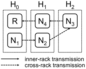
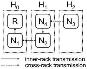
(a) No rack awareness	(b) With rack awareness

Figure 5: Repair pipelining with rack-aware path selection.

Algorithm 1 Rack-Aware Path Selection

1:

2:

3:identify the racks $\{H_{i}\}$ where the requestor $R$ and $n-1$ available helpers reside

4:let $H_{0}$ be the rack containing $R$ (and some helpers)

5:let $H_{1},H_{2},\cdots,H_{h}$ be the remote racks containing the remaining helpers, sorted by the number of helpers in a rack in descending order

6:$P=R$

7:$i=0$

8:while $P$ has fewer than $k$ helpers do

9:    for each helper $N$ in $H_{i}$ do

10:         $P=N\rightarrow P$

11:         if $P$ has $k$ helpers then

12:             break the while loop

13:         end if

14:    end for

15:    $i=i+1$

16:end while

17:return $P$

To make repair pipelining rack-aware, we require that the linear path of $k$ helpers has at most one incoming transmission and at most one outgoing transmission for each rack, while minimizing the total number of cross-rack transmissions. Algorithm 1 shows the pseudo-code of the rack-aware path selection. Specifically, to repair a failed block of a stripe, we identify a requestor $R$ and the remaining $n-1$ available helpers of the stripe. Let $H_{i}$ ($i\geq 0$) denote a rack where either $R$ or any helper resides, such that $H_{0}$ denotes the rack that contains $R$ (and possibly other helpers), $H_{1},H_{2},\cdots,H_{h}$ denote a total of $h$ remote racks that do not contain $R$ but contain the remaining helpers. Without loss of generality, we sort the number of helpers in the remote racks $H_{i}$’s ($1\leq i\leq h$) in descending order, where $|H_{1}|\geq|H_{2}|\geq\cdots\geq|H_{h}|$, and $|H_{i}|$ ($1\leq i\leq h$) denotes the number of helpers in $H_{i}$. We first initialize the linear path $P$ with only the requestor $R$ (Line 4). We then iteratively append a helper in $H_{i}$ to $P$, starting from $i=0$, until $P$ has $k$ helpers for reconstructing the failed block (Lines 5-14). Figure 5(b) shows a linear path for $k=4$ with rack-aware path selection.

Our rationale is that we prefer to append all helpers that are co-located with $R$ in $H_{0}$ to $P$, so as to involve only inner-rack transmissions. Also, when choosing helpers from the remote racks $H_{1},H_{2},\cdots,H_{h}$, we prefer to append as many helpers as possible in one rack to $P$, so as to minimize the number of remote racks to be accessed. Thus, we first choose helpers from $H_{1}$, followed by $H_{2}$, and so on. By minimizing the number of remote racks being accessed for a single-block repair, we also minimize the amount of cross-rack repair traffic under RS codes (see CAR [48]). Based on the analysis in §3, the single-block repair time still approaches one timeslot, while a timeslot here refers to the time of transmitting one block over a cross-rack link.

Remarks:

A recent work LAR [53] solves for a minimum spanning tree that takes the network distances among nodes as input and minimizes the cross-rack repair traffic in the network core of a hierarchical topology. For the special case where all nodes share the identical network distance to the network core, LAR can also return a linear path with the minimum cross-rack repair traffic as Algorithm 1. Unlike LAR, which uses network distances as input, Algorithm 1 uses only the block locations in different racks (as in CAR [48]) as input to find the linear path. Repair pipelining takes one step further to reduce the single-block repair time based on the returned linear path.

4.3 Weighted Path Selection

We now study a more diverse heterogeneous setting in which the link bandwidth can have any arbitrary value. In the following, we extend repair pipelining to solve a weighted path selection problem. Here, we focus on degraded reads, and discuss how we address full-node recovery.

Formulation:

Recall that for a single-block repair, repair pipelining transmits a number of slices along a linear path of $k$ helpers, say $N_{1}\rightarrow N_{2}\rightarrow\cdots\rightarrow N_{k}\rightarrow R$. Suppose that the link bandwidth is different across links. If the number of slices is sufficiently large, then the slices are transmitted in parallel through the path (Figure 3), and the performance of repair pipelining will be bottlenecked by the link with the minimum available bandwidth along the path. To minimize the single-block repair time, we should find a path that maximizes the minimum link bandwidth.

To repair a failed block of a stripe, we need to find $k$ out of $n-1$ available helpers of the same stripe as the failed block, and also find the sequence of link transmissions so that the path along the $k$ selected helpers and the requestor minimizes the single-block repair time. Specifically, there are a total of $n$ nodes, including the $n-1$ available helpers and the requestor. We associate a weight with each (directed) link from one node to another node, such that a higher weight implies a longer transmission time along the link. For example, the weight can be represented by the inverse of the link bandwidth obtained by periodic measurements on link utilizations [13]. Then our objective is to find a path of $k+1$ nodes (i.e., $k$ selected helpers and the requestor) that minimizes the maximum link weight of the path. Here, we focus on link weights, and the same idea is applicable if we associate weights with nodes. Any straggler is assumed to be associated with a large weight, so it will be excluded from the selected path.

To solve the above problem, a naïve approach is to perform a brute-force search on all possible candidate paths. However, there are a total of $\tfrac{(n-1)!}{(n-1-k)!}$ permutations, and the brute-force search becomes computationally expensive even for moderate sizes of $n$ and $k$. Since the link weights vary over time, the path selection should be done quickly on-the-fly based on the measured link weights.

Algorithm 2 Weighted Path Selection

1:

2:

3:procedure Main

4:    $P=R$

5:    $P^{*}=$ null

6:    $w^{*}=\infty$

7:    $\mathcal{N}=$ set of $n-1$ available helpers

8:    ExtendPath

9:    return $P^{*}$

10:end procedure

11:function ExtendPath

12:    if $P$.length $<k+1$ then

13:         for each node $N\in\mathcal{N}$ not in $P$ do

14:             if weight($N$, beginning node of path $P$) $<w^{*}$ then

15:                 $P=N\rightarrow P$

16:                 ExtendPath

17:                 remove $N$ from $P$

18:             end if

19:         end for

20:    else

21:         $P^{*}=P$

22:         $w^{*}=$ maximum link weight of $P$

23:    end if

24:end function

Algorithm:

We present a fast yet optimal algorithm that quickly identifies an optimal path. The algorithm builds on brute-force search to ensure that all candidate paths are covered, but eliminates the search of infeasible paths. Our insight is that if a link $L$ has a weight larger than the maximum weight of an optimal path candidate that is currently found, then we no longer need to search for the paths containing link $L$, since the maximum weight of any path containing $L$ must be larger than the maximum weight of the optimal path candidate.

Algorithm 2 shows the pseudo-code of the weighted path selection algorithm. Let $P$ be the path that we currently consider, $P^{*}$ be the optimal path candidate that we have found, $w^{*}$ be the maximum link weight of $P^{*}$, and $\mathcal{N}$ be the set of $n-1$ available helpers. We first initialize a path $P$ with only the requestor $R$ (Line 2), such that $R$ will be the end node of $P$. We also initialize $P^{*}$, $w^{*}$, and $\mathcal{N}$ (Lines 3-5). We call the recursive function ExtendPath (Line 6) and finally return the optimal path $P^{*}$ (Line 7).

The function ExtendPath recursively extends $P$ by one helper in $\mathcal{N}$ and appends the helper to $P$ if the link weight from the node to the current beginning node of $P$ is less than $w^{*}$; otherwise, the path containing the link cannot minimize the maximum link weight as argued above. Specifically, the algorithm appends $N\in\mathcal{N}$ to $P$ if the current path length is less than $k+1$ and the weight from $N$ to the beginning node of $P$ is less than $w^{*}$ (Lines 10-13). It calls ExtendPath again to consider candidate paths that now include $N\rightarrow P$ (Line 14). It then removes $N$ from $P$ (Line 15), and tries other nodes in $\mathcal{N}$. If the length of $P$ is now $k+1$, it implies that all of its links have weight less than $w^{*}$, so we update $P$ as the new optimal path $P^{*}$ and $w^{*}$ as the maximum link weight of $P^{*}$ (Lines 19-20).

Algorithm 2 significantly reduces the search time. We evaluate the search time for (14,10) codes using Monte-Carlo simulations over 1,000 runs on a machine with 3.7 GHz Intel Xeon E5-1620 v2 CPU and 16 GiB memory. The brute-force search takes 27 s on average, while Algorithm 2 reduces the search time to only 0.9 ms.

Remarks:

To address full-node recovery (§3.3), we apply Algorithm 2 to each stripe. If we apply greedy scheduling on helper selection, we simply substitute $\mathcal{N}$ with the set of $k$ selected helpers. Note that the brute-force search for the optimal path on the $k$ selected helpers remains expensive, since it considers $k!$ permutations on the sequence of link transmissions along the path. Thus, Algorithm 2 still significantly saves the search time in this case.

We emphasize that Algorithm 2 should not be viewed as a generalization of our rack-aware path selection in Algorithm 1 (§4.2) as both algorithms target different problem settings: Algorithm 1 specifically minimizes the number of cross-rack transmissions, while Algorithm 2 minimizes the maximum link weight of the linear path of helpers. Nevertheless, we can still apply Algorithm 2 in a geo-distributed environment (§6.2).

4.4 Multi-Block Repair

Finally, we show how repair pipelining simultaneously reconstructs multiple failed blocks of a stripe and reduces the multi-block repair time. Here, we only focus on homogeneous environments, and discuss how we can address the heterogeneous environments.

We first define the notation. Let $f$, where $1\leq f\leq n-k$, be the number of failed blocks of a stripe for an $(n,k)$ code, and $B_{1}^{*},B_{2}^{*},\cdots,B_{f}^{*}$ be the failed blocks to be reconstructed. Let $R_{1},R_{2},\cdots,R_{f}$ be the $f$ requestors where the failed blocks are reconstructed. Before issuing the repair, we first identify $k$ helpers of the stripe (say, $N_{1},N_{2},\cdots,N_{k}$) and their $k$ corresponding available blocks (say, $B_{1},B_{2},\cdots,B_{k}$, respectively). Each failed block $B_{j}^{*}$ ($1\leq j\leq f$) can be reconstructed via the linear combination $B_{j}^{*}=\sum_{i=1}^{k}a_{i,j}B_{i}$, where $a_{i,j}$’s $(1\leq i\leq k$, $1\leq j\leq f$) are the decoding coefficients specified by a given erasure code.

A straightforward multi-block repair approach is to invoke repair pipelining for a single-block repair over a linear path of $k$ helpers as described in §3.2 $f$ times, one for each failed block. Thus, the multi-block repair time approaches $f$ timeslots under the homogeneous link assumption, where a timeslot is the time for transmitting one block over a network link. However, each helper needs to read its locally stored block for each single-block repair, so it reads $f$ times its locally stored block in total. In the following, we re-design a multi-block repair approach in which each helper needs to read its locally stored block only once.

As in §3.2, we start with a naïve pipelining approach that realizes a multi-block repair without slicing, and show its limitations. Specifically, we arrange the $k$ helpers in a linear path, i.e., $N_{1}\rightarrow N_{2}\rightarrow\cdots\rightarrow N_{k}$, and connect $N_{k}$ to all $f$ requestors $R_{1},R_{2},\cdots,R_{f}$. To repair the $f$ failed blocks $\{B_{1}^{*},B_{2}^{*},\cdots,B_{f}^{*}\}$, $N_{1}$ uses its own block $B_{1}$ to compute a set of $f$ blocks $\{a_{1,1}B_{1},a_{1,2}B_{1},\cdots,a_{1,f}B_{1}\}$, where each $a_{1,j}B_{1}$ ($1\leq j\leq f$) is an input term to the linear combination for reconstructing $B_{j}^{*}$. $N_{1}$ sends the set of $f$ blocks to $N_{2}$. Then $N_{2}$ combines the received blocks with its own block $B_{2}$ and sends a new set of $f$ blocks $\{a_{1,1}B_{1}+a_{2,1}B_{2},a_{1,2}B_{1}+a_{2,2}B_{2},\cdots,a_{1,f}B_{1}+a_{2,f}B_{2}\}$ to $N_{3}$. The process repeats, and finally $N_{k}$ reconstructs all $f$ failed blocks $\{B_{1}^{*},B_{2}^{*},\cdots,B_{f}^{*}\}$ and sends them to the $f$ requestors. Note that each of the $k$ helpers reads its own block only once. For the total repair time, recall that a block-level transmission over a network link takes one timeslot. Thus, the whole repair incurs $f\times k$ timeslots, including $f(k-1)$ timeslots from $N_{1}$ to $N_{k}$ and $f$ timeslots from $N_{k}$ to all $f$ requestors. From this example, we observe that this naïve pipelining approach is even worse than conventional repair (which takes $k+f-1$ timeslots as shown in §2.2).

We now extend the above naïve pipelining approach with slicing and show how repair pipelining works for a multi-block repair. Repair pipelining decomposes each failed block $B_{j}^{*}$ ($1\leq j\leq f$) into $s$ slices denoted by $S_{j,1},S_{j,2},\cdots,S_{j,s}$. It pipelines the repair of the first set of $f$ slices of the $f$ failed blocks (i.e., $S_{1,1},S_{2,1},\cdots,S_{f,1}$) through a linear path, followed by the second set of $f$ slices (i.e., $S_{1,2},S_{2,2},\cdots,S_{f,2}$), and so on. In general, each helper pipelines the repair of $f$ slices at the same offset of the $f$ failed blocks along a linear path. Each set of $f$ slices will be reconstructed at $N_{k}$ (i.e., the last helper of the linear path), which then forwards the reconstructed slices to the $f$ requestors. Figure 6 shows how repair pipelining works for $k=4$, $s=6$, and $f=2$. Again, each of the $k$ helpers reads its locally stored block only once during the repair.

We now analyze the time complexity of repair pipelining for repairing $f$ failed blocks under the homogeneous link assumption. Again, we assume that the overheads due to computation and disk I/O are negligible compared to network transmission (§3.2). To repair a set of $f$ slices along a linear path, each helper sends $f$ slices to the next helper, or to all $f$ requestors for the last helper $N_{k}$. Thus, each transmission now takes $\tfrac{f}{s}$ timeslots. Following the analysis in §3.2, the total repair time of repairing $f$ failed blocks is $(s-1+k)\times\tfrac{f}{s}=f(1+\tfrac{k-1}{s})$ timeslots, which approaches $f$ timeslots if $s$ is sufficiently large. Thus, repair pipelining always incurs less repair time than conventional repair (which takes $k+f-1$ timeslots).

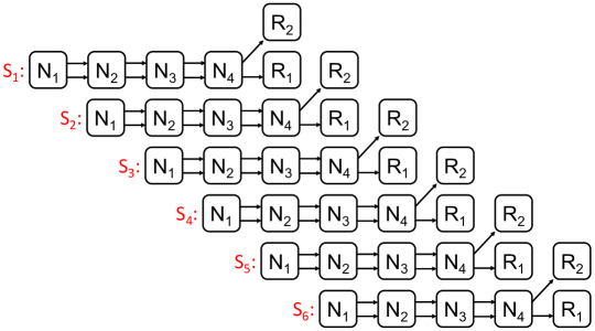
Figure 6: Repair pipelining for a multi-block repair with $k=4$, $s=6$, and $f=2$.

Remarks:

For a heterogeneous environment where network links have arbitrary bandwidth (§4.3), we discuss two possible solutions to realize a multi-block repair. One solution is to extend our proposed design, in which we aggregate all $f$ requestors as one big requestor, and assign a weight from each of the $n-f$ available helpers to the big requestor. Then we find an optimal linear path that minimizes the maximum link weight as in §4.3. An alternative solution is to call a single-block repair for each of the $f$ failed blocks and find an optimal path for each single-block repair as in §4.3. We pose the analysis for the possible solutions as future work.

5 Implementation

We have implemented a prototype called ECPipe to realize repair pipelining. ECPipe runs as a middleware atop an existing distributed storage system and performs repair operations on behalf of the storage system. Moving the repair logic to ECPipe greatly reduces changes to the code base of the storage system in order to realize new repair techniques; in the meantime, we can focus on optimizing ECPipe to maximize the repair performance gain. We have integrated ECPipe with three open-source distributed storage systems, namely HDFS-RAID [1], HDFS-3 [2], and QFS [35]. Both HDFS-RAID and HDFS-3 are written in Java, while QFS is written in C++. Our ECPipe prototype is mostly written in C++, and the parts for the integration into HDFS-RAID and HDFS-3 are in Java. Our ECPipe prototype has around 6,000 lines of code. The latest source code of ECPipe is available at: http://adslab.cse.cuhk.edu.hk/software/ecpipe.

5.1 Background of HDFS-RAID, HDFS-3, and QFS

We first provide the background details of HDFS-RAID, HDFS-3, and QFS. In particular, we describe how they support erasure coding.

HDFS-RAID

: HDFS-RAID is an erasure coding extension of Hadoop 0.20 HDFS. In this work, we choose Facebook’s HDFS-RAID implementation [1]. Specifically, the original HDFS comprises a NameNode for storage management and multiple DataNodes for actual storage. HDFS-RAID deploys a RaidNode atop HDFS for erasure coding management. It performs offline encoding (i.e., asynchronously in the background), in which HDFS initially stores data in DataNodes as fixed-size blocks (64 MiB by default) with replication, and the RaidNode later encodes replicated blocks into coded blocks via MapReduce [15].

The RaidNode also checks for any failed (lost or corrupted) coded block by verifying block checksums. It repairs any failed block being detected, either by itself in local mode or via a MapReduce job in distributed mode. Both modes will issue reads to $k$ available blocks of the same stripe in parallel from HDFS, reconstruct the failed block, and write back to HDFS. HDFS-RAID also provides a RAID file system client to access coded blocks. For a degraded read to a failed block, the RAID file system reads $k$ available blocks of the same stripe in parallel and reconstructs the failed block.

HDFS-3:

HDFS-3 (Hadoop 3.1.1 HDFS) [2] includes erasure coding in HDFS storage by design. Unlike HDFS-RAID, HDFS-3 performs online encoding (i.e., on the write path), in which an HDFS client performs encoding before writing data to storage. Specifically, the HDFS client first writes data into $k$ data buffers (with the default size of 1 MiB) and encodes them into $n-k$ parity buffers. It then appends the $n$ buffers into $n$ blocks in different DataNodes. Compared to offline encoding in HDFS-RAID, online encoding in HDFS-3 removes the extra I/O costs of reading and encoding the currently stored data blocks. However, it now moves the encoding overhead to the client, which performs encoding and writes the data and parity blocks to HDFS storage.

The NameNode monitors any failed blocks via the periodic block reports issued from DataNodes. If a failed block exists, the NameNode assigns a repair task to a DataNode, which issues parallel reads to $k$ available blocks from other DataNodes, reconstructs the failed block, and writes the reconstructed block back to HDFS-3.

QFS:

QFS stores all data in erasure-coded format and currently supports (9,6) RS codes [43]. Similar to HDFS-3, QFS performs online encoding. Specifically, a QFS client writes data into six 1 MiB buffers. It then encodes the six 1 MiB buffers into three 1 MiB parity buffers, and appends the nine 1 MiB buffers to nine data and parity blocks (the default block size is 64 MiB) that are stored in different storage nodes (called ChunkServers). To repair any failed block, a ChunkServer retrieves six available blocks from other ChunkServers for reconstruction.

5.2 ECPipe Design

Figure 7 shows the ECPipe architecture. It uses a coordinator to manage the repair operation between a requestor and multiple helpers. ECPipe runs atop a distributed storage system. To repair a failed block, the storage system creates a requestor instance, which sends a repair request with the failed block ID to the coordinator (step 1). The coordinator uses the failed block ID to identify the locations of $k$ available blocks of the same stripe. It notifies all helpers with the block locations (step 2). The helpers retrieve the blocks, perform repair pipelining in slices, and deliver the repaired slices to the requestor (step 3).

Note that if there are multiple failed blocks in a stripe, the storage system creates multiple requestor instances, each of which issues the failed block ID of one of the failed blocks to the coordinator. Again, the coordinator selects $k$ helpers to perform a multi-block repair via repair pipelining, so that the failed blocks are reconstructed in multiple requestors.

We integrate ECPipe with a storage system in three aspects. First, we implement the requestor as a class (in C++ and Java) that can be instantiated by the storage system to reconstruct failed blocks. For HDFS-RAID, the requestor is created in either the RaidNode or the RAID file system client; for HDFS-3 and QFS, it is created by the storage node that starts a repair operation. Second, we implement each helper as a daemon that is co-located with each storage node to directly read the locally stored blocks. Our insight is that HDFS-RAID, HDFS-3, and QFS all store a block in the underlying native file system as a plain file and use the block ID to form the file name. Thus, each helper can directly read the stored blocks via the native file system. This eliminates the need of helpers to fetch data through the distributed storage system routine. It not only reduces the burden of metadata management of the distributed storage system, but also improves the repair performance (§6.3). Finally, the coordinator needs to access both the block locations and the mappings of each block to its stripe. For HDFS-RAID, we retrieve the information from the RaidNode; for HDFS-3, we retrieve the information from the NameNode; for QFS, we retrieve the information from a storage node when it starts a repair operation.

To simplify our implementation, ECPipe uses Redis [4] to pipeline slices across helpers. Each helper maintains an in-memory key-value store based on Redis, and uses the client interface of Redis to transmit slices among helpers. In addition, each helper performs disk I/O, network transfer, and computation via multiple threads for performance speedup. Adding ECPipe into HDFS-RAID, HDFS-3, and QFS only requires changes of around 110, 245, and 180 lines of code, respectively.

To provide fair comparisons (§6), we also implement conventional repair (§2.2) and PPR [31] under the same ECPipe framework, by only changing the transmission flow of data during a repair.

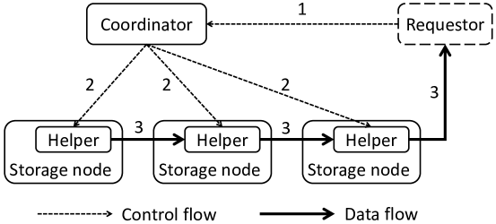
Figure 7: ECPipe architecture.

6 Evaluation

We conduct experiments on both a local cluster and Amazon EC2. We show that repair pipelining outperforms both conventional repair and PPR [31] under various settings. We further show that our repair pipelining implementation in ECPipe outperforms different baseline repair pipelining implementations.

6.1 Evaluation on a Local Cluster

Methodology: We first evaluate ECPipe as a standalone system on a local cluster. Our local cluster comprises 17 machines, each of which has a quad-core 3.4 GHz Intel Core i5-3570 CPU, 16 GiB RAM, and a Seagate ST1000DM003-1CH162 1 TiB SATA hard disk. We host the coordinator on one machine and 16 helpers on the remaining ones. By default, all machines are connected via a 1 Gb/s Ethernet switch. The 1 Gb/s bandwidth can be viewed as modeling the cross-rack bandwidth available for repair tasks in a production cluster [45], in which the blocks of a stripe are stored in distinct racks. We also connect the machines via a 10 Gb/s Ethernet switch and evaluate ECPipe in higher network speeds (Figures 8(h) and 8(i)).

Initially, we store coded blocks in the local file system of each machine, and load block locations and stripe information into the coordinator. We simulate a “failed” machine by erasing its stored blocks, and repair the failed block of each stripe in a requestor. We host the requestor on a machine that does not store any available block of the repaired stripe, so as to ensure that the available blocks are always transmitted over the network. By default, we configure 64 MiB block size, 32 KiB slice size, and (14,10) RS codes; note that (14,10) RS codes are also used by Facebook [45, 42]. We vary one of the settings at a time and evaluate its impact.

We mainly compare the basic version of repair pipelining described in §3 with conventional repair (§2) and PPR [31]. We focus on three key repair metrics:

• Single-block repair time: the latency from issuing a degraded read request to a failed block until the block is reconstructed;

• Full-node recovery rate: the ratio of the amount of recovered data in a failed node to the total repair time; and

• Multi-block repair time: the latency from issuing a request of repairing multiple failed blocks in a stripe until they are all reconstructed.

All results are averaged over 10 runs. We find that the standard deviations are small and hence omit them from the plots.

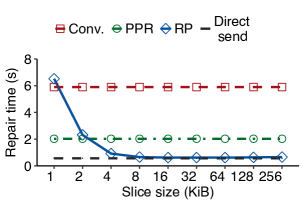
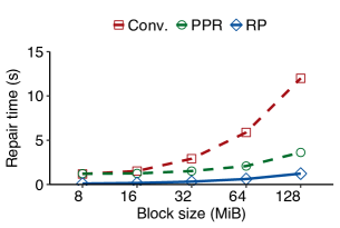
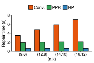
(a) Slice size	(b) Block size	(c) Coding parameters
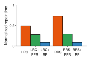
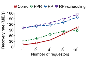
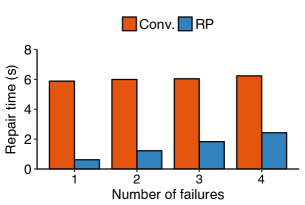
(d) Repair-friendly codes	(e) Full-node recovery	(f) Multi-block repair
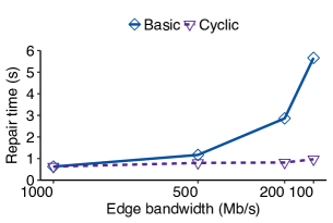
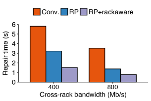
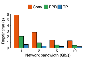
(g) Limited edge bandwidth	(h) Rack awareness	(i) Varying network bandwidth

Figure 8: Evaluation on a local cluster.

Slice size:

Figure 8(a) shows the single-block repair time versus the slice size in repair pipelining; for fair comparisons, we also partition the blocks into 32 KiB slices in both conventional repair and PPR, so that they can also exploit parallelism for better performance. We further plot the transmission time of directly sending a single block over a 1 Gb/s link (labeled as “Direct send”). From the figure, we see that repair pipelining shows high repair time when the slice size is small, even though more slices are pipelined during a repair (i.e., $s$ is small). The reason is that the overhead of issuing transmission requests for many slices becomes significant. We see that the repair time decreases as the slice size increases up to 32 KiB (where $s=$ 2,048), and then increases since there are too few slices in a block being pipelined (i.e., less parallelization). When the slice size is 32 KiB, repair pipelining reduces the single-block repair time by 89.5% and 69.5% compared to conventional repair and PPR, respectively.

Also, the direct send time of transferring a 64 MiB block is 0.57s, which is almost network-bound in our 1 Gb/s network. The single-block repair time of repair pipelining is only 8.8% more than the direct send time. This shows the feasibility of reducing the single-block repair time to almost the same as the normal read time for a single available block.

Block size:

Figure 8(b) shows the single-block repair time versus the block size. Repair pipelining reduces the single-block repair time by 88.8-91.6% and 66.0-91.8% compared to conventional repair and PPR, respectively.

Coding parameters:

Figure 8(c) shows the single-block repair time versus $(n,k)$. The single-block repair time of conventional repair significantly increases with $k$, while that of PPR also increases with $k$ (albeit less significantly than in conventional repair). On the other hand, the single-block repair time of repair pipelining remains almost unchanged. As $k$ increases from 6 to 12, the repair time reduction of repair pipelining increases from 82.5% to 91.2% compared to conventional repair, and from 68.6% to 70.4% compared to PPR.

Repair-friendly codes:

We demonstrate how repair pipelining is compatible with practical erasure codes. We consider two state-of-the-art repair-friendly codes: Local Reconstruction Codes (LRC) [23] and Rotated RS codes [26]. LRC partitions the data blocks into local groups and associates a local parity block with each local group of data blocks. It improves the performance of a single-block repair, which can now be done within a local group, at the expense of higher storage redundancy. On the other hand, Rotated RS codes arrange the layout of parity blocks to improve the performance of a degraded read to a series of data blocks. We configure LRC with $k=$ 12 data blocks that are partitioned in two local groups with six blocks each, and Rotated RS codes with $(n,k)=$ (16,12). LRC reads only six available blocks within a local group for repairing a failed block, while Rotated RS codes on average read nine blocks for repairing a failed block.

Figure 8(d) shows the normalized single-block repair time with respect to conventional repair of (16,12) RS codes. The normalized single-block repair time of repair pipelining (around 0.1) is much smaller than those of LRC and Rotated RS codes by effectively utilizing the bandwidth resources of all helpers. We observe the same improvement in PPR, but its repair time reduction is less than that of repair pipelining.

Full-node recovery:

We now evaluate full-node recovery with multiple requestors and our greedy scheduling in helper selection (§3.3). Specifically, we randomly write multiple stripes of blocks across all 16 helpers in the local cluster. We erase 64 blocks from 64 stripes (one block per stripe) in one helper to mimic a single node failure, and recover all the erased blocks simultaneously. We distribute the reconstructed blocks evenly across a number of requestors, varied from one to 16. Each requestor is deployed in a distinct machine.

We consider two cases of helper selection in repair pipelining: (i) we index the helpers from 1 to 16, and always select the available blocks from the $k$ helpers that have the smallest indexes in a stripe for repair (labeled as “RP”); and (ii) we use the greedy approach to select $k$ helpers that are least recently accessed for repair (labeled as “RP+scheduling”). We also evaluate conventional repair and PPR, both of which select helpers without greedy scheduling.

Figure 8(e) shows the full-node recovery rates. As the number of requestors increases, the recovery rates of all schemes increase. Conventional repair sees the largest gain by distributing the repair load across more requestors. Interestingly, as the number of requestors increases to 16, conventional repair even achieves a slightly higher recovery rate than PPR. However, repair pipelining still outperforms conventional repair by making bandwidth utilization more balanced. Furthermore, our greedy scheduling achieves an observable gain when there are a large number of requestors. For example, when there are eight (resp. 16) requestors, the recovery rate of repair pipelining without greedy scheduling is 1.89$\times$ (resp. 1.51$\times$) that of conventional repair, and our greedy scheduling further increases the recovery rate of repair pipelining by 13.3% (resp. 8.9%).

Multi-block repair:

Figure 8(f) shows the multi-block repair time versus the number of failed blocks in a stripe. Here, we compare repair pipelining and conventional repair only, and omit PPR as its design does not address the multi-block repair of a stripe. Conventional repair has relatively stable repair time (ranging from 5.88 s to 6.23 s) regardless of the number of failed blocks being repaired, as it always retrieves $k$ available blocks for repairing the failed blocks of a stripe. On the other hand, the repair time of repair pipelining almost increases linearly with the number of failed blocks. Nevertheless, repair pipelining still has 60.9% less repair time than conventional repair for a four-block repair.

Limited edge bandwidth:

Our previous tests focus on homogeneous environments, and we now move our evaluation to heterogeneous environments. We show the benefits of the cyclic version when a requestor sits at the network edge and the edge bandwidth from the storage system to the requestor is limited (§4.1). Specifically, we use the Linux tc command [5] to limit the edge bandwidth from each helper to the requestor. We compare the cyclic version with the basic version in §3.

Figure 8(g) shows the single-block repair time versus the edge bandwidth. When the edge bandwidth is 1 Gb/s (i.e., the homogeneous case), both the basic and cyclic versions have almost identical repair time. As the edge bandwidth decreases, the repair time of the basic version increases significantly, while that of the cyclic version only increases mildly by allowing the requestors to read the reconstructed data from multiple helpers in parallel. For example, the cyclic version has 82.8% less repair time than the basic version when the edge bandwidth is 100 Mb/s.

Rack awareness:

We evaluate repair pipelining in a rack-based data center scenario. Specifically, we configure (9,6) RS codes. We divide our cluster into three logical racks, and use the Linux tc command [5] to limit the cross-rack bandwidth. We distribute the $n=9$ blocks of each stripe evenly across the three logical racks (i.e., $n/3=3$ blocks per rack), so that the block placement can tolerate any single-rack failure. We compare repair pipelining with and without rack awareness (§4.2), as well as conventional repair; we do not consider PPR here as its design does not address rack awareness.

Figure 8(h) shows the single-block repair time in two cross-rack bandwidth settings: 400 Mb/s and 800 Mb/s. Repair pipelining without rack awareness reduces the repair time of conventional repair, yet with rack awareness, we observe a further drop of the single-block repair time. For example, when the cross-rack bandwidth is 800 Mb/s, repair pipelining without rack awareness reduces the single-block repair time of conventional repair by 60.9%; with rack awareness, the reduction further improves to 77.6% since the cross-rack repair traffic is minimized.

Varying network bandwidth:

We evaluate repair pipelining when the network bandwidth is above 1 Gb/s, in which the computation and disk I/O overheads become significant. We now connect all machines in our local cluster via a 10 Gb/s Ethernet switch. We use the Linux tc command [5] to vary the available network bandwidth of each node (up to 10 Gb/s).

Figure 8(i) shows that single-block repair time versus the network bandwidth. As the available network bandwidth increases, the single-block repair time decreases in all schemes. Also, the repair time reduction of repair pipelining also drops due to the more significant overheads in both computation and disk I/O. Nevertheless, repair pipelining still shows a performance gain. For example, when the network bandwidth is 10 Gb/s, repair pipelining reduces the single-block repair time by 81.4% and 50.0% compared to conventional repair and PPR, respectively (while the reduction reaches around 90% and 70% when the network bandwidth is 1 Gb/s, as shown in Figure 8(a)).

6.2 Evaluation on Amazon EC2

Methodology: We evaluate ECPipe on Amazon EC2. Specifically, we consider geo-distributed clusters that span multiple geographic regions [17, 6, 12], in which erasure-coded blocks are striped across regions to protect against large-scale correlated failures. We evaluate ECPipe on two Amazon EC2 clusters, one in North America and one in Asia. Table 1 shows one of our iperf [3] measurement tests for the inner-region and cross-region bandwidth values on Amazon EC2 across four regions respectively in North America and Asia. We observe that the inner-region bandwidth is in general more abundant than the cross-region bandwidth, and the cross-region bandwidth has a high degree of variance.

Bandwidth	California	Canada	Ohio	Oregon
California	501.3	57.2	44.1	299.9
Canada	55.3	732.0	63.3	48.0
Ohio	46.3	65.7	332.5	95.6
Oregon	297.8	50.2	93.6	250.1

(a) North America

Bandwidth	Mumbai	Seoul	Singapore	Tokyo
Mumbai	624.8	62.3	39.5	37.7
Seoul	63.8	265.7	86.1	183.2
Singapore	41.5	88.1	493.0	49.1
Tokyo	39.7	181.0	46.9	489.1

(b) Asia

Table 1: An iperf test of inner- and cross-region bandwidth measurements (in Mb/s) on Amazon EC2 in North America and Asia. Each value is the measured bandwidth from the row region to the column region. Note that the bandwidth values fluctuate across different tests.

We deploy four EC2 instances per region per cluster to host helpers (i.e., 16 helpers in total), and one EC2 instance in Ohio and Singapore to host the coordinator for the North America and Asia clusters, respectively. Note that the overhead of accessing the coordinator has negligible impact on the overall repair performance. We focus on evaluating the single-block repair time of a degraded read issued by a requestor. We host the requestor on an EC2 instance in each region and study how the performance varies across regions. All EC2 instances are of type t2.micro.

We configure 64 MiB block size and 32 KiB slice size for repair pipelining. We use (16,12) RS codes and distribute the 16 blocks of each stripe across the 16 EC2 instances in four regions; this also provides fault tolerance against any single-region failure. We consider two versions of repair pipelining: the basic version in §3 (labeled as “RP”), which finds a random path across $k$ randomly selected helpers, and the optimal version in §4.3 (labeled as “RP+optimal”), which finds an optimal path via Algorithm 2. Note that the network bandwidth fluctuates over time, although inner-region bandwidth remains higher than cross-region bandwidth, as shown in Table 1. Thus, the optimal version probes the network bandwidth via iperf before each run of experiments. We average our results over 10 runs, and also include the standard deviations as the results have higher variances than in our local cluster.

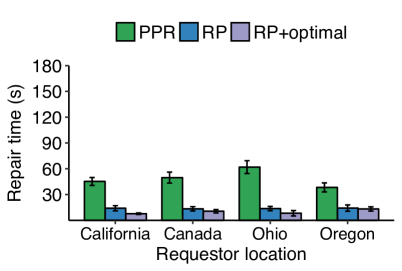
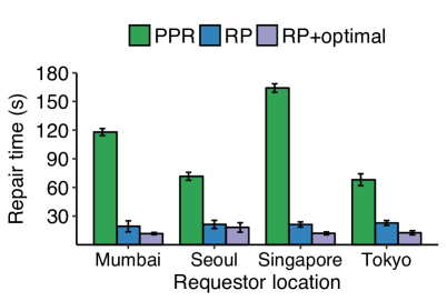
(a) North America cluster	(b) Asia cluster

Figure 9: Evaluation on Amazon EC2.

Results:

Figure 9 shows the single-block repair time and the standard deviations of PPR and the two versions of repair pipelining in both clusters; we do not show the results of conventional repair, whose repair time goes beyond 200 s. Repair pipelining (without weighted path selection) achieves repair time saving over PPR in all cases when the requestor is in different regions. The repair time reduction is 62.7-78.0% for North America and 66.6-87.1% for Asia. Our weighted path selection further reduces the repair time by 7.3-45.4% for North America and 14.5-45.0% for Asia, compared to repair pipelining without weighted path selection. Note that our weighted path selection can be done in around 1 ms (§4.3), which is negligible compared to the repair time in our evaluation.

6.3 Evaluation on HDFS-RAID, HDFS-3, and QFS

Methodology: We evaluate the integration of ECPipe into HDFS-RAID, HDFS-3, and QFS, all of which are deployed in our local cluster (§6.1). We co-locate a helper daemon with each of the 16 storage nodes (i.e., DataNodes in HDFS-RAID and HDFS-3, or ChunkServers in QFS). By default, we set the slice size of repair pipelining as 32 KiB and block size as 64 MiB. For HDFS-RAID and HDFS-3, we vary $(n,k)$, while for QFS, we use its default (9,6) RS codes and vary the slice size and block size. We consider three repair schemes: (i) the original repair implementations of HDFS-RAID, HDFS-3 and QFS, all of which are based on conventional repair, (ii) the conventional repair under ECPipe, and (iii) the basic version of repair pipelining in §3 under ECPipe.

For HDFS-RAID and QFS, we evaluate degraded reads (in single-block repair time) issued by a requestor that is attached with either an HDFS-RAID client or a QFS ChunkServer. For HDFS-3, we observe similar results of the single-block repair time as in HDFS-RAID. Thus, we focus on evaluating full-node recovery in HDFS-3, in which we evenly distribute 64 stripes of blocks across all DataNodes, followed by erasing all blocks of a DataNode and repairing the lost blocks in a new DataNode. We report the averaged results over 10 runs as in §6.1 (the standard deviations are small and omitted).

Results:

Figure 10 shows the evaluation results. First, repair pipelining under ECPipe significantly improves the repair performance of the original repair implementations of HDFS-RAID, HDFS-3, and QFS. Specifically, for HDFS-RAID, repair pipelining reduces the single-block repair time by 82.7-91.2% for different $(n,k)$ (Figure 10(a)); for HDFS-3, it achieves 5.1-16.0$\times$ full-node recovery rate for different $(n,k)$ (Figure 10(b)); for QFS, it reduces the single-block repair time by up to 86.6% when the slice size is 32 KiB and the block size is 64 MiB (Figures 10(c) and 10(d)).

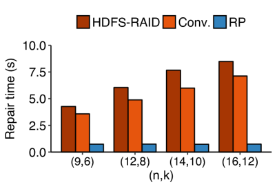
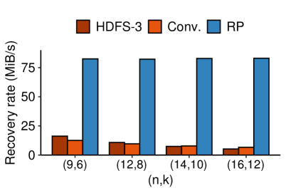
(a) HDFS-RAID: single-block repair time versus coding parameters	(b) HDFS-3: full-node recovery rate versus coding parameters
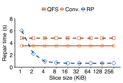
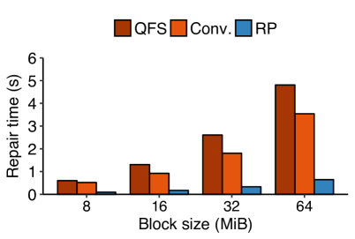
(c) QFS: single-block repair time versus slice size	(d) QFS: single-block repair time versus block size

Figure 10: Evaluation on HDFS-RAID, HDFS-3, and QFS.

We observe that moving the repair logic to ECPipe improves single-block repair performance. Specifically, conventional repair under ECPipe reduces the single-block repair time by up to 21.8% and 26.3% in HDFS-RAID and QFS, respectively, compared to the original conventional repair implementation. The reason of the performance gain is that the helpers of ECPipe can directly access the stored blocks via the native file system, instead of fetching the blocks through the distributed storage system routine. For full-node recovery, conventional repair under ECPipe outperforms the original conventional repair when $k$ is large (i.e., $k=$ 10 or 14). The reason is that when $k$ increases, the overhead of initiating connections to $k$ DataNodes for retrieving available blocks in HDFS-3 also increases. Nevertheless, we emphasize that the repair performance gain mainly comes from repair pipelining, rather than the implementation of ECPipe. Although moving repair to ECPipe reduces the repair time, the reduction is minor compared to the reduction achieved by repair pipelining.

6.4 Evaluation of Different Repair Pipelining Implementations

Methodology: We compare different repair pipelining implementations based on ECPipe in our local cluster (§6.1). First, we compare the block-level and slice-level repair pipelining approaches, and implement two baseline variants called Pipe-B and Pipe-S. Pipe-B implements block-level repair pipelining (i.e., without slicing) along a linear path of helpers, each of which sends a partially repaired block to the next helper (or the requestor for the last helper); in essence, Pipe-B is the naïve approach as described in §3.2. Pipe-S implements slice-level repair pipelining without parallelization. It realizes the sub-operations of repairing a slice inside a helper (i.e., receiving the partially repaired slice from the preceding helper, reading its locally stored slice, computing a new partially repaired slice, and sending the partially repaired slice) in a serial manner. Our current repair pipelining implementation (referred to as RP) also performs slice-level repair pipelining. Compared to Pipe-S, RP carefully parallelizes the sub-operations of slices in each helper to simultaneously utilize all available resources. Note that RP is our default implementation used in the previous experiments (§6.1-§6.3).

We also compare our repair pipelining implementation with the design in PUSH [24] in full-node recovery as described in §6.1 (note that PUSH does not consider single-block repair). As the source code of PUSH is unavailable, we implement the two variants of PUSH, namely PUSH-Rep and PUSH-Sur, in ECPipe based on the description of the paper [24], which we refer to them as Pipe-Rep and Pipe-Sur, respectively. Both Pipe-Rep and Pipe-Sur implement block-level repair pipelining. Pipe-Rep reconstructs all failed blocks in a single node, while Pipe-Sur distributes the reconstructed blocks across all 16 nodes in our local cluster in a round-robin manner. For comparisons, we consider two variants of our repair pipelining implementation (with greedy scheduling enabled), namely RP-single and RP-all. RP-single reconstructs all failed blocks in a single node, while RP-all distributes all reconstructed blocks across all 16 nodes in our local cluster. Both RP-single and RP-all are configured with 16 requestors: for RP-single, we deploy all 16 requestors in the node where the failed blocks are reconstructed; for RP-all, we deploy one requestor per node. Compared to PUSH-Rep and PUSH-Sur, both RP-single and RP-all implement slice-level repair pipelining.

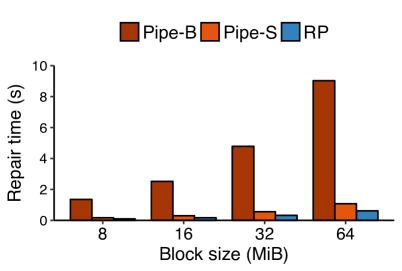
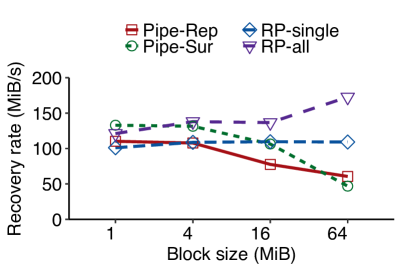
(a) Single-block repair time versus block size	(b) Full-node recovery rate versus block size

Figure 11: Evaluation on different repair pipelining implementations.

Results:

Figure 11 shows the results, averaged over 10 runs. Figure 11(a) evaluates the single-block repair time versus the block size for Pipe-B, Pipe-S, and RP, where both Pipe-S and RP have the slice size fixed as 32 KiB. Pipe-B has the largest single-block repair time (e.g., 9.0 s for repairing a 64 MiB block), while Pipe-S significantly reduces the single-block repair time (e.g., 1.1 s for repairing a 64 MiB block) through slice-level repair pipelining. This again shows that slice-level repair pipelining can improve the repair performance via more fine-grained parallelization. RP further reduces the single-block repair time (e.g., 0.61 s for repairing a 64 MiB block) by carefully scheduling the slice-level repair sub-operations in a parallel fashion. Overall, RP reduces the single-block repair time of Pipe-S by 41.1-43.0% across all block sizes. Note that we observe similar performance differences between Pipe-S and RP for different slice sizes, so we omit the results here.

Figure 11(b) evaluates the full-node recovery rate versus the block size for Pipe-Rep, Pipe-Sur, RP-single, and RP-all. Here, we repair 4 TiB of lost data (i.e., the number of reconstructed blocks is 4 TiB divided by the block size), and fix the slice size for RP-single and RP-all as 32 KiB. We observe that when the block size is 1 MiB, both Pipe-Rep and Pipe-Sur have higher recovery rates than RP-single and RP-all by 9.0% and 9.7%, respectively. The reason is that Pipe-Rep and Pipe-Sur benefit from block-level repair pipelining across a large number of blocks in small block sizes. On the other hand, in RP-single and RP-all, each block is only divided into a limited number of slices (e.g., 32 slices for a 1 MiB block). They do not benefit much from slice-level repair pipelining.

Nevertheless, as the block size increases, the recovery rates of both Pipe-Rep and Pipe-Sur drop significantly, as the number of blocks decreases for larger block sizes and the performance gain from pipelining is limited. On the other hand, the recovery rates of RP-single and RP-all increase with the block size, as each block can now be divided into more slices. Both RP-single and RP-all can benefit from the slice-level repair pipelining for each block; note that they also allow multiple requestors to reconstruct the lost blocks in parallel. When the block size is 64 MiB, the recovery rates of RP-single and RP-all are 80.2% and 268.1% higher than those of Pipe-Rep and Pipe-Sur, respectively. Also, RP-all has a higher recovery rate than RP-single (e.g., by 58.1% when the block size is 64 MiB) by distributing the repair load across the requestors in different nodes. In summary, our current repair pipelining implementation maintains its high performance gain in large block sizes, which are commonly found in state-of-the-art distributed storage systems (e.g., 64 MiB [18] or 256 MiB [42]).

7 Related Work

Many new erasure codes have been proposed in the literature to mitigate repair overhead, especially for a single-node repair. To name a few, regenerating codes [16] minimize the repair traffic by allowing storage nodes to send encoded data during a single-node repair. Rotated RS codes [26] reduce the repair traffic and disk I/O of a degraded read to a sequence of data blocks. Hitchhiker [42] extends RS codes [43] to piggyback parity information of one stripe into another stripe, and is shown to reduce the repair traffic and I/O by up to 45%. PM-RBT codes [40] are special regenerating codes that simultaneously minimize the repair traffic, disk I/O, and storage redundancy. Butterfly codes [36] are systematic regenerating codes that provide double-fault tolerance. Clay codes [51] couple multiple layers of MDS codes and achieve optimality in terms of the repair traffic, disk I/O, storage redundancy, as well as the sub-packetization level (i.e., the number of sub-blocks divided within a block). Locally repairable codes [23, 45] add local parity blocks to mitigate repair I/O with extra storage redundancy.

Instead of constructing new erasure codes, we design new repair strategies for general practical erasure codes. Some prior studies are also along this direction. Tree-structured data regeneration [27] specifically targets regenerating codes [16], and constructs a spanning tree that maximizes the bandwidth utilization during repair. Lazy repair [10, 50] defers immediate repair action until a tolerable limit is reached. To speed up full-node recovery, the repair of multiple stripes can be parallelized across available nodes, as also adopted by replicated storage [14, 34] and de-clustered RAID arrays [20]. Degraded-first scheduling [28] targets MapReduce on erasure-coded storage by scheduling map tasks to fully utilize bandwidth in degraded reads. FastPR [46] reconstructs in advance the data stored in soon-to-fail nodes, so as to speed up the repair operation. A closely related work to ours is PPR [31], which reduces the single-block repair time from $k$ timeslots to $\lceil\log_{2}(k+1)\rceil$ timeslots by parallelizing partial repair operations across different nodes, while repair pipelining reduces the single-block repair time to one timeslot.

Several studies improve the repair performance of erasure-coded storage for hierarchical data centers. Some studies [22, 39, 21] propose new regenerating codes that minimize the cross-rack repair traffic for hierarchical topologies, in which storage nodes are organized in racks. CAR [48] minimizes the cross-rack repair traffic for RS-coded storage by first computing partial repaired results in each rack and then sending the partial repaired results across racks. LAR [53], similar to CAR [48], also studies how to minimize the cross-rack repair traffic in the network core of a hierarchical topology by solving for a minimum spanning tree. ClusterSR [47] not only minimizes the cross-cluster repair traffic in geo-distributed storage, but also balances the upload and download traffic in full-node recovery. With hierarchy awareness, repair pipelining preserves the minimum cross-rack repair traffic and further reduces the single-block repair time (§4.2).

Some studies also propose pipelined approaches to improve the repair performance in erasure-coded storage. PUSH [24] forms a reconstruction chain along different helpers and performs block-level repair pipelining for full-node recovery. In contrast, our repair pipelining design schedules a single-block repair at a more fine-grained slice level, and we show that how it substantially reduces the single-block repair time to almost the same as the normal read time for a single block. Compared to PUSH, our contributions include: (i) by slicing a block (a read/write unit of a distributed storage system) into smaller units, we show that repair pipelining can reduce the degraded read time for an unavailable block to almost the same as the normal read time for an available block (in contrast, PUSH only focuses on full-node recovery); (ii) we present extensions of repair pipelining for heterogeneous environments; (iii) we show how repair pipelining can be readily integrated via ECPipe into existing distributed storage systems (i.e., HDFS-RAID, HDFS-3, and QFS); and (iv) we compare different repair pipelining implementations (including our own implementation of PUSH [24]). LAR [53] implements pipelined reconstruction by dividing blocks into packets (i.e., slices in our case). However, it does not formally analyze how the packets are scheduled to minimize single-block repair time. Parallel Pipeline Tree (PPT) [9] constructs an optimized repair tree based on repair pipelining for heterogeneous environments, while we address some special cases of heterogeneous environments, such as the scenario where the link bandwidth between the storage system and the requestor is limited as well as hierarchical data centers. Our recent work, OpenEC [30], provides a framework that simplifies the deployment of repair pipelining through a directed-acyclic-graph abstraction.

8 Conclusions

Repair pipelining is a general technique that reduces the single-block repair time to almost the same as the normal read time for a single available block in erasure-coded storage. It schedules the repair of a failed block across storage nodes in units of slices in a pipelined manner, so as to evenly distribute the repair traffic and fully utilize bandwidth resources across storage nodes. Our contributions include: (i) the design of repair pipelining for both degraded reads and full-node recovery, (ii) the extensions of repair pipelining with parallel reads, hierarchy awareness, and weighted path selection for heterogeneous environments, (iii) the extension of repair pipelining for repairing multiple failed blocks in a stripe, (iv) a repair prototype ECPipe and its integrations into HDFS-RAID, HDFS-3, and QFS, and (v) the local cluster and Amazon EC2 experiments that show the repair speedup through repair pipelining.

References

- [1] Facebook’s Hadoop. https://github.com/facebookarchive/hadoop-20, Retrieved in November 2020.
- [2] Hadoop 3.1.1 HDFS. https://hadoop.apache.org/docs/r3.1.1/, Retrieved in November 2020.
- [3] Iperf. https://iperf.fr/, Retrieved in November 2020.
- [4] Redis. http://redis.io/, Retrieved in November 2020.
- [5] tc. https://linux.die.net/man/8/tc, Retrieved in November 2020.
- [6] M. K. Aguilera. Geo-distributed storage in data centers, 2013. Slides presented at International Conference on Principles of Distributed Systems (OPODIS’13).
- [7] F. Ahmad, S. T. Chakradhar, A. Raghunathan, and T. Vijaykumar. ShuffleWatcher: Shuffle-aware scheduling in multi-tenant Mapreduce clusters. In Proceedings of the 2014 USENIX Annual Technical Conference (USENIX ATC’14), pages 1–12, 2014.
- [8] F. André, A.-M. Kermarrec, E. L. Merrer, N. L. Souarnec, G. Straub, and A. van Kempen. Archiving cold data in warehouses with clustered network coding. In Proceedings of the Ninth European Conference on Computer Systems (EuroSys’14), pages 1–14, 2014.
- [9] Y. Bai, Z. Xu, H. Wang, and D. Wang. Fast recovery techniques for erasure-coded clusters in non-uniform traffic network. In Proceedings of the 48th International Conference on Parallel Processing (ICPP’19), pages 1–10, 2019.
- [10] R. Bhagwan, K. Tati, Y. Cheng, S. Savage, and G. Voelker. Total Recall: System support for automated availability management. In Proceedings of the First Symposium on Networked Systems Design and Implementation (NSDI’04), page 25, 2004.
- [11] B. Calder, J. Wang, A. Ogus, N. Nilakantan, A. Skjolsvold, S. McKelvie, Y. Xu, S. Srivastav, J. Wu, H. Simitci, et al. Windows Azure Storage: A highly available cloud storage service with strong consistency. In Proceedings of the 23rd ACM Symposium on Operating Systems Principles (SOSP’11), pages 143–157, 2011.
- [12] Y. Chen, S. Mu, J. Li, C. Huang, J. Li, A. Ogus, and D. Phillips. Giza: Erasure coding objects across global data centers. In Proceedings of the 2017 USENIX Annual Technical Conference (USENIX ATC’17), pages 539–551, 2017.
- [13] M. Chowdhury, S. Kandula, and I. Stoica. Leveraging endpoint flexibility in data-intensive clusters. In Proceedings of the ACM SIGCOMM 2013 conference (SIGCOMM’13), pages 231–242, 2013.
- [14] B. Chun, F. Dabek, A. Haeberlen, E. Sit, H. Weatherspoon, M. F. Kaashoek, J. Kubiatowicz, and R. Morris. Efficient replica maintenance for distributed storage systems. In Proceedings of the 3rd Symposium on Networked Systems Design & Implementation (NSDI’06), pages 45–58, 2006.
- [15] J. Dean and S. Ghemawat. MapReduce: Simplified data processing on large clusters. In Proceedings of the 6th Symposium on Opearting Systems Design & Implementation (OSDI’04), pages 137–149, 2004.
- [16] A. G. Dimakis, P. B. Godfrey, Y. Wu, M. Wainwright, and K. Ramchandran. Network coding for distributed storage systems. IEEE Transactions on Information Theory, 56(9):4539–4551, Sep 2010.
- [17] D. Ford, F. Labelle, F. I. Popovici, M. Stokel, V.-A. Truong, L. Barroso, C. Grimes, and S. Quinlan. Availability in globally distributed storage systems. In Proceedings of the 9th USENIX Symposium on Operating Systems Design and Implementation (OSDI’10), pages 61–74, 2010.
- [18] S. Ghemawat, H. Gobioff, and S. Leung. The Google File System. In Proceedings of the 19th ACM Symposium on Operating Systems Principles (SOSP’03), pages 29–43, 2003.
- [19] C. A. R. Hoare. Algorithm 65: find. Communications of the ACM, 4(7):321–322, 1961.
- [20] M. Holland and G. A. Gibson. Parity declustering for continuous operation in redundant disk arrays. In Proceedings of the 5th International Conference on Architectural Support for Programming Languages and Operating Systems (ASPLOS’92), pages 23–35, 1992.
- [21] H. Hou, P. P. C. Lee, K. W. Shum, and Y. Hu. Rack-aware regenerating codes for data centers. IEEE Transactions on Information Theory, 65(8):4730–4745, Aug 2019.
- [22] Y. Hu, X. Li, M. Zhang, P. P. Lee, X. Zhang, P. Zhou, and D. Feng. Optimal repair layering for erasure-coded data centers: From theory to practice. ACM Transactions on Storage, 13(4):1–24, 2017.
- [23] C. Huang, H. Simitci, Y. Xu, A. Ogus, B. Calder, P. Gopalan, J. Li, and S. Yekhanin. Erasure coding in Windows Azure storage. In Proceedings of the 2012 USENIX Annual Technical Conference (USENIX ATC’12), pages 15–26, 2012.
- [24] J. Huang, X. Liang, X. Qin, Q. Cao, and C. Xie. PUSH: A pipelined reconstruction I/O for erasure-coded storage clusters. IEEE Transactions on Parallel and Distributed Systems, 26(2):516–526, 2015.
- [25] V. Jalaparti, P. Bodik, I. Menache, S. Rao, K. Makarychev, and M. Caesar. Network-aware scheduling for data-parallel jobs: Plan when you can. In Proceedings of the ACM SIGCOMM 2015 conference (SIGCOMM’15), pages 407–420, 2015.
- [26] O. Khan, R. Burns, J. Plank, W. Pierce, and C. Huang. Rethinking erasure codes for cloud file systems: Minimizing i/o for recovery and degraded reads. In Proceedings of the 10th USENIX conference on File and Storage Technologies (FAST’12), pages 251–264, 2012.
- [27] J. Li, S. Yang, X. Wang, and B. Li. Tree-structured data regeneration in distributed and storage systems with regenerating codes. In Proceedings of the 29th IEEE Conference on Computer Communications (INFOCOM’10), pages 2892–2900, 2010.
- [28] R. Li, P. P. C. Lee, and Y. Hu. Degraded-first scheduling for MapReduce in erasure-coded storage clusters. In Proceedings of the 44th Annual IEEE/IFIP International Conference on Dependable Systems and Networks (DSN’14), pages 419–430, 2014.
- [29] R. Li, X. Li, P. P. C. Lee, and Q. Huang. Repair pipelining for erasure-coded storage. In Proceedings of the 2017 USENIX Annual Technical Conference (USENIX ATC’17), pages 567–579, 2017.
- [30] X. Li, R. Li, P. P. C. Lee, and Y. Hu. OpenEC: Toward unified and configurable erasure coding management in distributed storage systems. In Proceedings of the 17th USENIX conference on File and Storage Technologies (FAST’19), pages 331–344, 2019.
- [31] S. Mitra, R. Panta, M.-R. Ra, and S. Bagchi. Partial-parallel-repair (PPR): A distributed technique for repairing erasure coded storage. In Proceedings of the 11th European Conference on Computer Systems (EuroSys’16), pages 1–16, 2016.
- [32] S. Muralidhar, W. Lloyd, S. Roy, C. Hill, E. Lin, W. Liu, S. Pan, S. Shankar, V. Sivakumar, L. Tang, and S. Kumar. f4: Facebook’s warm BLOB storage system. In Proceedings of the 11th USENIX Symposium on Operating Systems Design and Implementation (OSDI’14), pages 383–398, 2014.
- [33] L. M. Ni and P. K. McKinley. A survey of wormhole routing techniques in direct networks. IEEE Computer, 26(2):62–76, 1993.
- [34] D. Ongaro, S. M. Rumble, R. Stutsman, J. Ousterhout, and M. Rosenblum. Fast crash recovery in RAMCloud. In Proceedings of the 23rd ACM Symposium on Operating Systems Principles (SOSP’11), pages 29–41, 2011.
- [35] M. Ovsiannikov, S. Rus, D. Reeves, P. Sutter, S. Rao, and J. Kelly. The Quantcast file system. Proceedings of the VLDB Endowment, 6(11):1092–1101, 2013.
- [36] L. Pamies-Juarez, F. Blagojević, R. Mateescu, C. Gyuot, E. E. Gad, and Z. Bandic. Opening the chrysalis: On the real repair performance of MSR codes. In Proceedings of the 14th Usenix Conference on File and Storage Technologies (FAST’16), pages 81–94, 2016.
- [37] J. S. Plank. Erasure codes for storage systems: A brief primer. ;login: the Usenix magazine, 38(6):44–50, Dec 2013.
- [38] J. S. Plank, J. Luo, C. D. Schuman, L. Xu, and Z. Wilcox-O’Hearn. A performance evaluation and examination of open-source erasure coding libraries for storage. In Proceedings of the 7th USENIX Conference on File and Storage Technologies (FAST’09), pages 253–265, 2009.
- [39] N. Prakash, V. Abdrashitov, and M. Médard. The storage versus repair-bandwidth trade-off for clustered storage systems. IEEE Transactions on Information Theory, 64(8):5783–5805, 2018.
- [40] K. V. Rashmi, P. Nakkiran, J. Wang, N. B. Shah, and K. Ramchandran. Having your cake and eating it too: Jointly optimal erasure codes for I/O, storage, and network-bandwidth. In Proceedings of the 13th USENIX Conference on File and Storage Technologies (FAST’15), pages 81–94, 2015.
- [41] K. V. Rashmi, N. B. Shah, D. Gu, H. Kuang, D. Borthakur, and K. Ramchandran. A solution to the network challenges of data recovery in erasure-coded distributed storage systems: A study on the Facebook warehouse cluster. In Proceedings of the 5th USENIX conference on Hot Topics in Storage and File Systems (HotStorage’13), page 8, 2013.
- [42] K. V. Rashmi, N. B. Shah, D. Gu, H. Kuang, D. Borthakur, and K. Ramchandran. A ”hitchhiker’s” guide to fast and efficient data reconstruction in erasure-coded data centers. In Proceedings of the ACM SIGCOMM 2014 conference (SIGCOMM’14), pages 331–342, 2014.
- [43] I. Reed and G. Solomon. Polynomial codes over certain finite fields. Journal of the Society for Industrial and Applied Mathematics, 8(2):300–304, 1960.
- [44] J. K. Resch and J. S. Plank. AONT-RS: Blending security and performance in dispersed storage systems. In Proceedings of the 9th USENIX conference on File and Storage Technologies (FAST’11), pages 191–202, 2011.
- [45] M. Sathiamoorthy, M. Asteris, D. Papailiopoulos, A. G. Dimakis, R. Vadali, S. Chen, and D. Borthakur. XORing elephants: Novel erasure codes for big data. Proceedings of the VLDB Endowment, 6(5):325–336, 2013.
- [46] Z. Shen, X. Li, and P. P. C. Lee. Fast predictive repair in erasure-coded storage. In Proceedings of the 49th Annual IEEE/IFIP International Conference on Dependable Systems and Networks (DSN’19), pages 556–567, 2019.
- [47] Z. Shen, J. Shu, Z. Huang, and Y. Fu. Clustersr: Cluster-aware scattered repair in erasure-coded storage. In Proceedings of the 35th IEEE International Parallel & Distributed Processing Symposium (IPDPS’20), pages 42–51, 2020.
- [48] Z. Shen, J. Shu, and P. P. C. Lee. Reconsidering single failure recovery in clustered file systems. In Proceedings of the 46th Annual IEEE/IFIP International Conference on Dependable Systems and Networks (DSN’16), pages 323–334, 2016.
- [49] K. Shvachko, H. Kuang, S. Radia, and R. Chansler. The Hadoop distributed file system. In Proceedings of the 2010 IEEE 26th Symposium on Mass Storage Systems and Technologies (MSST’10), pages 1–10, 2010.
- [50] M. Silberstein, L. Ganesh, Y. Wang, L. Alvizi, and M. Dahlin. Lazy means smart: Reducing repair bandwidth costs in erasure-coded distributed storage. In Proceedings of International Conference on Systems and Storage (SYSTOR’14), pages 1–7, 2014.
- [51] M. Vajha, V. Ramkumar, B. Puranik, G. Kini, E. Lobo, B. Sasidharan, P. V. Kumar, A. Barg, M. Ye, S. Narayanamurthy, et al. Clay codes: Moulding MDS codes to yield an MSR code. In Proceedings of the 16th USENIX Conference on File and Storage Technologies (FAST’18), pages 139–154, 2018.
- [52] H. Weatherspoon and J. D. Kubiatowicz. Erasure coding vs. replication: A quantitative comparison. In Proceedings of the first International Workshop on Peer-to-Peer Systems (IPTPS’02), pages 328–337, 2002.
- [53] F. Xu, Y. Wang, X. Pei, and X. Ma. LAR: Locality-aware reconstruction for erasure-coded distributed storage systems. Concurrency and Computation: Practice and Experience, 31(11):e5031, 2019.