Recognizing and realizing cactus metrics

Abstract

The problem of realizing finite metric spaces in terms of weighted graphs has many applications. For example, the mathematical and computational properties of metrics that can be realized by trees have been well-studied and such research has laid the foundation of the reconstruction of phylogenetic trees from evolutionary distances. However, as trees may be too restrictive to accurately represent real-world data or phenomena, it is important to understand the relationship between more general graphs and distances. In this paper, we introduce a new type of metric called a cactus metric, that is, a metric that can be realized by a cactus graph. We show that, just as with tree metrics, a cactus metric has a unique optimal realization. In addition, we describe an algorithm that can recognize whether or not a metric is a cactus metric and, if so, compute its optimal realization in $O(n^{3})$ time, where $n$ is the number of points in the space.

1 Introduction

The metric realization problem, which is the problem of representing a finite metric space by a weighted graph, has many applications, most notably in the reconstruction of evolutionary trees. Although any finite metric space can be realized by a weighted complete graph, there can be different graphs that induce the same metric. In [8], Hakimi and Yau first considered “optimal” realizations of finite metric spaces, which are realizations of least total weight. Although every finite metric space has an optimal realization [6, 12], the problem of finding an optimal realization is NP-hard in general [1, 17] and the optimal solution is not necessarily unique [1, 6].

A well-known special case of optimal realizations is provided by tree metrics, namely, those metrics that can be realized by some edge-weighted tree. For any tree metric on a finite set $X$, its optimal realization is an $X$-tree (i.e., a tree in which some vertices are labeled by $X$) and is uniquely determined [8]. In addition, there exist optimal polynomial-time algorithms for computing the tree realization from a tree metric [3, 4, 5]. However, not much is known about the properties of optimal realizations of metrics induced by graphs that are more general than trees. Developing our understanding in this direction could be useful, as trees can sometimes be too restrictive for realizing metrics arising in real-world applications [11].

In this paper, we generalize the concept of a tree metric by introducing a new type of metric called a “cactus metric” which can be realized by an edge-weighted “$X$-cactus”, where a cactus is a connected graph in which each edge belongs to at most one cycle. An example of an $X$-cactus is presented in Figure 1. Note that cacti have some nice properties in common with trees. For instance, every cactus is planar and the number of vertices in an $X$-cactus is $O(|X|)$ as with $X$-trees, which means that cactus metrics are easy to visualize. In particular, they provide a special case of an open problem in discrete geometry from Matoušek [13]. Besides these observations, in this paper we prove that, just as with tree metrics, any cactus metric has a unique optimal realization. We also describe a polynomial time algorithm for deciding whether or not an arbitrary metric is a cactus metric, which also computes its optimal realization in case it is.

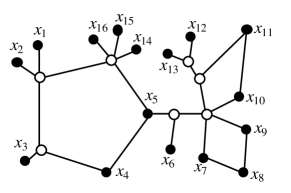
Figure 1: An example of an $X$-cactus with a label-set $X=\{x_{1},\dots,x_{16}\}$, where the weight of each edge is proportional to its length. The vertices labeled by an element of $X$ are shown in black. The white circles are vertices that are not in $X$.

2 Preliminaries

A metric on a set $S$ is defined to be a function $d:S\times S\to{\mathbb{R}}_{\geq 0}$ with the property that $d$ equals zero if and only if the two elements in $S$ are identical, is symmetric, and satisfies the triangle inequality.

All graphs considered here are finite, connected, simple, undirected graphs in which the edges have positive weights. For any graph $G$, $V(G)$ and $E(G)$ represent the vertex-set and edge-set of $G$, respectively. For any vertex $v$ of a graph $G$, the number of edges of $G$ that have $v$ as an endvertex is denoted by $deg(v)$. For any graph $G$ and any subset $S$ of $V(G)$, we let $d_{G}$ denote the metric on $S$ induced by taking shortest paths in $G$ between elements in $S$.

Throughout this paper, we use the symbol $X$ to represent a finite set with $|X|\geq 2$, which is sometimes called a label-set. For any metric $d$ on $X$, a realization of $(X,d)$ is a graph $G$ such that $X$ is a subset of $V(G)$ and $d(x,y)=d_{G}(x,y)$ holds for each $x,y\in X$, where we shall always assume that each vertex $v$ of $G$ with $deg(v)\leq 2$ has a label in $X$ [12]. A realization is minimal if the removal of an arbitrary edge of $G$ yields a graph that does not realize $d$. It is optimal if the sum of its edge weights is minimum over all possible realizations (note that optimal realizations are minimal but the converse does not hold). Any finite metric space has at least one optimal realization [12, Theorem 2.2].

We now state a theorem concerning optimal realizations which will be useful in our proofs. For a graph $G$, each maximal biconnected subgraph of $G$ is called a block of $G$ and each vertex of $G$ shared by two or more blocks of $G$ is called a cutvertex of $G$. Notice that if a graph consists of a single block, then it has no cutvertex.

Theorem 1 ([12], Theorem 5.9)

Let $G$ be a minimal realization of a finite metric space $(X,d)$, let $G_{1},\dots,G_{k}$ be the blocks of $G$, let $M_{i}$ be the union of the vertices of $X$ in $G_{i}$ together with the cutvertices of $G$ in $G_{i}$, and let $d_{i}$ be the metric induced by $G$ on $M_{i}$. Then, if every $G_{i}$ is an optimal realization of $(M_{i},d_{i})$, then $G$ is also optimal. If every $G_{i}$, besides being optimal, is also unique, then $G$ is optimal and unique too.

We now turn to two special classes of metrics, that is, tree metrics and cyclelike metrics. A metric $d$ on $X$ is called a tree metric if there exists an $X$-tree that realizes $(X,d)$, where an $X$-tree is a tree $T$ with the property that each vertex $v$ of $T$ with $deg(v)\leq 2$ is contained in $X$ [14].

Theorem 2 ([8])

If $d$ is a tree metric on a finite set $X$, then there exists an $X$-tree that is a unique optimal realization of $(X,d)$.

Given a metric $d$ on $X$ with $|X|\geq 4$, we say that $d$ is cyclelike if there is a minimal realization for $d$ that is a cycle. This type of metric was discussed in e.g., [2, 12, 15]. The following result will also be useful.

Theorem 3 ([12], Theorem 4.4)

Suppose $d$ is a cyclelike metric on a finite set $X$ and a cycle $C$ is a minimal realization of $(X,d)$ with $V(C)=X=\{v_{1},v_{2},\dots,v_{m}\}$, $m\geq 4$, and $E(C)=\{\{v_{i},v_{i+1}\}\,:\,1\leq i\leq m\}$, where the indices are taken modulo $m$. Then, $C$ is an optimal realization of $(X,d)$ if and only if

$$d(v_{i-1},v_{i})+d(v_{i},v_{i+1})=d(v_{i-1},v_{i+1})$$

holds for all $i$. In this case, $C$ is the unique optimal realization of $(X,d)$.

3 The uniqueness of optimal realizations of cactus metrics

As mentioned above a cactus is a connected graph in which each edge belongs to at most one cycle. We define an $X$-cactus to be a cactus $G$ with the property that each vertex $v$ of $G$ with $deg(v)\leq 2$ is contained in $X$ (see Figure 1). Note that the maximum number of cycles in an $X$-cactus is $|X|-2$ (which can be proved by induction on $|X|$). In addition, we say that a metric $d$ on a finite set $X$ is a cactus metric if there exists an edge-weighted $X$-cactus that realizes $(X,d)$.

Given an edge-weighted cycle $C=v_{1},\dots,v_{m}$ that is a realization of its corresponding metric $d_{C}$, we call a vertex $v_{i}\in V(C)$ slack if $d(v_{i-1},v_{i})+d(v_{i},v_{i+1})>d(v_{i-1},v_{i+1})$. The following lemma is a direct consequence of Theorem 3.

Lemma 4

Under the premise of Theorem 3, $C$ is an optimal realization of $(X,d)$ if and only if $C$ has no slack vertex.

We now use the lemma to prove the following generalization of Theorem 2, using the concept of “compactification” [8, 15, 16].

Theorem 5

If $d$ is a cactus metric on a finite set $X$, then there exists an $X$-cactus that is a unique optimal realization of $(X,d)$.

Proof: Let $G$ be an $X$-cactus that is a minimal realization of $(X,d)$. Without loss of generality, we assume that each cycle of $G$ has at least four vertices (since we can always replace a 3-cycle with a tree in such a way that the obtained graph is a realization). If there is no cycle in $G$ containing a slack vertex, then the assertion immediately follows from Theorems 1, 3 and Lemma 4.

So, assume that there is a cycle $C=v_{1},\dots,v_{m}$ in $G$ that has consecutive edges $\{v_{i-1},v_{i}\},\{v_{i},v_{i+1}\}$ with $\Delta_{i}:=\{d_{G}(v_{i-1},v_{i})+d_{G}(v_{i},v_{i+1})-d_{G}(v_{i-1},v_{i+1})\}/2>0$. As we will now explain, we apply a “compactification” operation to the slack vertex $v_{i}$ (see also Figure 2). For notational convenience, let $\Delta_{i-1}:=\{d_{G}(v_{i-1},v_{i})+d_{G}(v_{i-1},v_{i+1})-d_{G}(v_{i},v_{i+1})\}/2$ and $\Delta_{i+1}:=\{d_{G}(v_{i+1},v_{i})+d_{G}(v_{i-1},v_{i+1})-d_{G}(v_{i},v_{i-1})\}/2$. Compactification of $v_{i}$ refers to converting $G$ into the graph $G^{\prime}$ with $V(G^{\prime}):=V(G)\cup\{v_{i}^{\prime}\}$ and $E(G^{\prime}):=(E(G)\setminus\{\{v_{i-1},v_{i}\},\{v_{i},v_{i+1}\}\})\cup\{\{v_{i-1},v_{i}^{\prime}\},\{v_{i},v_{i}^{\prime}\},\{v_{i+1},v_{i}^{\prime}\}\}$, where for each $j\in\{i-1,i,i+1\}$, the edge $\{v_{j},v_{i}^{\prime}\}$ has weight $\Delta_{j}$. As can be easily verified, $G^{\prime}$ is an $X$-cactus that is a minimal realization of $(X,d)$ with a strictly smaller number of slack vertices than $G$. Thus, as $|V(G)|$ is finite, by applying the same operation repeatedly and suppressing all unlabeled vertices of degree two (if any arise), we will eventually obtain an $X$-cactus that realizes $(X,d)$ without a slack vertex, which must be the unique optimal realization of $(X,d)$.

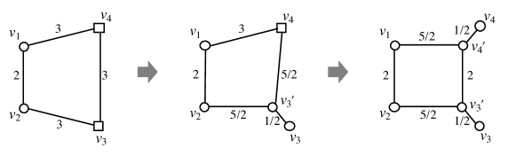
Figure 2: An illustration of compactification that is described in the proof of Theorem 5, where we highlight each slack vertex by a square. Compactification of $v_{3}$ in the left graph yields the graph in the middle panel, which still contains a slack vertex $v_{4}$. If we further apply the same operation to $v_{4}$, then we obtain the graph on the right which has no slack vertex.

It is interesting to see that for cactus metrics, we do not need to perform too many “compactifications” for each cycle in the above proof in light of the following observation.

Proposition 6

If the premise of Theorem 3 holds, then $C$ has at most two slack vertices. In the case when there exist precisely two slack vertices, they are adjacent in $C$.

Proof: Let $V(C)=\{v_{1},\dots,v_{m}\}$ as in Theorem 3. Suppose $C$ has at least two slack vertices and assume that $v_{i}$ is a slack vertex, in other words, that $d(v_{i-1},v_{i})+d(v_{i},v_{i+1})>d(v_{i-1},v_{i+1})$ holds. As the path in $C$ from $v_{i-1}$ to $v_{i+1}$ that does not contain $v_{i}$ is the shortest path between $v_{i-1}$ and $v_{i+1}$, it follows that any $v\in V(C)\setminus\{v_{i-1},v_{i},v_{i+1}\}$ is not slack. Now, suppose $v_{i-1}$ is a slack vertex. Then using a similar argument by considering the shortest path between $v_{i-2}$ and $v_{i}$, it follows that $v_{i+1}$ is not slack. So the only slack vertices are $v_{i}$ and $v_{i-1}$. The same argument applies to the case when $v_{i+1}$ is a slack vertex.

4 A polynomial time algorithm for finding the optimal cactus realization

In this section we describe an algorithm, which for a metric $d$ on $X$, produces the unique optimal realization for $d$ that is an $X$-cactus or a message that there is no such realization in $O(|X|^{3})$ time. This should be compared to tree metrics for which the same process can be carried out in $O(|X|^{2})$ time [4, 5].

We begin by considering cyclelike metrics. Note that the characterization given in Theorem 3 for when a realization of a cyclelike metric is optimal is not sufficient to characterize cyclelike metrics, as pointed out in [15]. Even so we have the following result (which is related to Theorem 4.1 in [2]):

Lemma 7

Given a metric $d$ on $X$, we can determine if there is an edge-weighted cycle $C$ that is an optimal realization of $(X,d)$ and, if so, compute $C$ in $O(|X|^{2})$ time.

Proof: We describe an algorithm that takes an arbitrary metric $d$ on $X$ as input, which in case $d$ has an optimal realization that is a cycle computes this cycle, and stops if this is not the case:

1) Start by finding a pair $\{v_{0},v_{1}\}$ of distinct elements in $X$ such that $d(v_{0},v_{1})\leq d(p,q)$ holds for any $\{p,q\}\in\binom{X}{2}\setminus\{\{v_{0},v_{1}\}\}$, and then set $e_{1}:=\{v_{0},v_{1}\}$ and $w_{1}:=d(v_{0},v_{1})$. 2) For each $j\in\{2,\dots,|X|-1\}$, find all vertices $x\in X\setminus\{v_{0},\dots,v_{j-1}\}$ with $d(v_{j-2},v_{j-1})+d(v_{j-1},x)=d(v_{j-2},x)$. Among these vertices, we let $v_{j}$ be the unique vertex $x$ that minimizes $d(v_{j-1},x)$. If such a vertex does not exist, or if such a vertex does exist but it is not unique, then stop; else set $e_{j}:=\{v_{j-1},v_{j}\}$ and $w_{j}:=d(v_{j-1},v_{j})$. 3) Set $e_{|X|}:=\{v_{|X|-1},v_{0}\}$ and $w_{|X|}:=d(v_{|X|-1},v_{0})$. 4) Check if the cycle $C$ defined by $V(C):=X$ and $E(C):=\{e_{1},\dots,e_{|X|}\}$ together with the weight $w_{j}$ of each edge $e_{j}\in E(C)$ is a minimal realization of $(X,d)$. If not then stop, else output the weighted cycle $C$.

If this algorithm returns a cycle $C$ that realizes $(X,d)$, then $C$ satisfies the equation in Theorem 3 and so $C$ is the optimal realization of $(X,d)$. Conversely, if there is a cycle $C$ that is an optimal realization of $(X,d)$, then $C$ is unique. In this case, the above algorithm correctly constructs $C$ as follows. The algorithm initializes by finding two vertices of $X$ that are closest together. Since an optimal realization that is a cycle is minimal, it must be the case that these two vertices are connected by an edge. In Step 2, the algorithm iteratively extends the existing path by seeking for the neighbour of $v_{j-1}$, which is one of the endvertices of the path. Observe that the two conditions in Step 2 uniquely determine this neighbour: the first condition ensures that a shortest path between $v_{j-2}$ and $v_{j}$ contains $v_{j-1}$; the second condition correctly identifies the neighbour of $v_{j-1}$ by making sure that the distance between it and $v_{j-1}$ is shortest. In Step 3, we join the two endvertices of the path by an edge to form the cycle $C$. Note that in this step, we run the risk of making a realization of $(X,d)$ that is a path into a realization of $(X,d)$ that is a cycle that is not minimal. Due to this, and also to ensure we have the correct solution, we check that the cycle is a minimal realization of $(X,d)$ in Step 4.

To give the running time of the algorithm, observe that Step 1 takes $O(|X|^{2})$ time as we search for a minimum element from a set of size $\binom{|X|}{2}$. In Step 2, we iterate over a ‘for loop’ at most $|X|$ times. Within the ‘for loop’ we iterate over at most $|X|$ elements to find the vertices that satisfy the first condition. Then, we iterate over those vertices to find a minimum element from at most $|X|$ elements. Hence, each ‘for loop’ takes $O(|X|)$ time; it follows then that Step 2 takes $O(|X|^{2})$ time. Step 3 takes constant time, as we simply add a weighted edge to the graph. Since one can obtain the metric induced by a cycle in at most $O(|X|^{2})$ time, Step 4 can be performed in at most $O(|X|^{2})$ time. As each step of the algorithm can be done in $O(|X|^{2})$ time, the whole algorithm requires $O(|X|^{2})$ time.

Theorem 8

Given a metric $d$ on $X$, we can determine if $d$ is a cactus metric and if so construct its optimal realization in $O(|X|^{3})$ time.

Proof: In [10, Algorithm 2] Hertz and Varone give a polynomial time algorithm for decomposing an arbitrary metric space $(X,d)$ into finite metric spaces $(M_{i},d_{i})$, $1\leq i\leq k$, with $|M_{i}|\leq|X|$, such that any optimal realization of $(M_{i},d_{i})$ must consist of a single block, and such that an optimal realization for $d$ can be constructed by piecing together the optimal realizations for the $(M_{i},d_{i})$. They also observe [10, p.174] that this decomposition can be computed in $O(|X|^{3})$ time using results in [7] (see also [7, p.160]). In addition, by the arguments in [7, Lemma 3.1], it follows that $k$ is $O(|X|)$.

Assume that we have decomposed $(X,d)$ into $\{(M_{i},d_{i})\}_{i\in\{1,\dots,k\}}$ by using the aforementioned preprocessing algorithm. In case $|M_{i}|=2$, its optimal realization is obviously a tree. Recalling the argument in the proof of Theorem 5, we know that $|M_{i}|\neq 3$ holds for each $i\in\{1,\dots,k\}$. For each $(M_{i},d_{i})$ with $|M_{i}|\geq 4$, by using the algorithm in Lemma 7, we can check if $(M_{i},d_{i})$ has an optimal realization that is a cycle or not, and if so construct the cycle in $O(|M_{i}|^{2})$ time (and hence $O(|X|^{2})$ time suffices). If there is some $i\in\{1,\dots,k\}$ such that $|M_{i}|\geq 4$ and $(M_{i},d_{i})$ does not have an optimal realization that is a cycle, then $d$ is not a cactus metric, else $d$ is a cactus metric, and we can construct the cactus by piecing together the optimal realizations for the $(M_{i},d_{i})$. Using the aforementioned fact that $k$ is $O(|X|)$, we conclude that the overall time complexity is $O(|X|^{3})$.

5 Discussion and future work

It may be worth investigating as to whether there is a more direct and efficient algorithm than the one given in Theorem 8 for recognizing and/or realizing cactus metrics that use structural properties of cactus graphs. More generally, we could investigate optimal realizations for metrics that can be realized by graphs $G$ in which every block $G_{i}=(V_{i},E_{i})$ satisfies $|E_{i}|-|V_{i}|+1\leq k$, and such that every vertex in $G$ with degree at most 2 is contained in $X$. Here, we note that in case $k=0$, $G$ is an $X$-tree, and in case $k=1$, $G$ is an $X$-cactus. However, even in case $k=2$, there may be infinitely many optimal realizations (e.g. the metric given in [1, Fig. 15]). So it might be interesting to first understand for $k\geq 2$ which of these metrics have a unique optimal realization, whether such metrics can be recognized in polynomial time, and whether there exists a polynomial time algorithm for computing some optimal realization.

Acknowledgment: Hayamizu is supported by JST PRESTO Grant Number JPMJPR16EB. Huber, Moulton and Murakami thank the Netherlands Organization for Scientific Research (NWO), including Vidi grant 639.072.602. Huber and Moulton also thank the Research Institute for Mathematical Sciences, Kyoto University, The Institute of Statistical Mathematics, Tokyo, and the London Mathematical Society for their support.

References

- [1] I.Althöfer, On optimal realizations of finite metric spaces by graphs, Discrete and Computational Geometry 3(1) (1988) 103-122.
- [2] A.Baldisserri, R.Elena, Distance matrices of some positive-weighted graphs, Australian Journal of Combinatorics 70(2) (2018) 185-201.
- [3] H.-J.Bandelt, Recognition of tree metrics, SIAM Journal on Discrete Mathematics 3(1) (1990) 1-6.
- [4] V.Batagelj, T.Pisanski, J.M.Simões-Pereira, An algorithm for tree-realizability of distance matrices, International Journal of Computer Mathematics 34(3-4) (1990) 171-176.
- [5] J.C.Culberson, P.Rudnicki, A fast algorithm for constructing trees from distance matrices, Information Processing Letters 30(4) (1989) 215-220.
- [6] A.Dress, Trees, tight extensions of metric spaces, and the cohomological dimension of certain groups: a note on combinatorial properties of metric spaces, Advances in Mathematics 53(3) (1984) 321-402.
- [7] A.Dress, K.T.Huber, J.Koolen, V.Moulton, A.Spillner, An algorithm for computing cutpoints in finite metric spaces, Journal of Classification 27(2) (2010) 158-172.
- [8] S.L.Hakimi, S.S.Yau, Distance matrix of a graph and its realizability, Quarterly of Applied Mathematics 22(4) (1965) 305-317.
-
[9]
M.Hayamizu,
-cactus trees and cactus tree metrics, The 21st New Zealand Phylogenomics Meeting (Waiheke 2017), 12-17 February 2017.
https://cdn.auckland.ac.nz/assets/compevol/events/
documents/Waiheke2017Programme.pdf - [10] A.Hertz, S.Varone, The metric cutpoint partition problem, Journal of Classification 25(2) (2008) 159-175.
- [11] D.H.Huson, R.Rupp, C.Scornavacca, Phylogenetic networks: concepts, algorithms and applications, Cambridge University Press, 2010.
- [12] W.Imrich, J.M.Simoes-Pereira, C.M.Zamfirescu, On optimal embeddings of metrics in graphs, Journal of Combinatorial Theory, Series B 36(1) (1984) 1-15.
- [13] J.Matoušek, 2.7 How large graph?, Open problems on embeddings of finite metric spaces Workshop on discrete metric spaces and their algorithmic applications, 2002, available at http://kam.mff.cuni.cz/ matousek/metrop.ps.
- [14] C.Semple, M.Steel, Phylogenetics, Oxford University Press, 2003.
- [15] J.M.S. Simões-Pereira, A note on distance matrices with unicyclic graph realizations, Discrete Mathematics 65(3) (1987) 277-287.
- [16] J.M.S. Simões-Pereira, C.M. Zamfirescu, Submatrices of non-tree-realizable distance matrices, Linear Algebra and its Applications 44 (1982) 1-17.
- [17] P.Winkler, The complexity of metric realization, SIAM Journal on Discrete Mathematics, 1(4) (1988) 552-559.