Probing of violation of Lorentz invariance
by ultracold neutrons in the Standard Model Extension

Abstract

We analyze a dynamics of ultracold neutrons (UCNs) caused by interactions violating Lorentz invariance within the Standard Model Extension (SME) (Colladay and Kostelecký, Phys. Rev. D 55, 6760 (1997) and Kostelecký, Phys. Rev. D 69, 105009 (2004)). We use the effective non–relativistic potential for interactions violating Lorentz invariance derived by Kostelecký and Lane (J. Math. Phys. 40, 6245 (1999)) and calculate contributions of these interactions to the transition frequencies of transitions between quantum gravitational states of UCNs bouncing in the gravitational field of the Earth. Using the experimental sensitivity of qBounce experiments we make some estimates of upper bounds of parameters of Lorentz invariance violation in the neutron sector of the SME which can serve as a theoretical basis for an experimental analysis. We show that an experimental analysis of transition frequencies of transitions between quantum gravitational states of unpolarized and polarized UCNs should allow to place some new constraints in comparison to the results adduced by Kostelecký and Russell in Rev. Mod. Phys. 83, 11 (2011); edition 2019, arXiv: 0801.0287v12 [hep-ph].

I Introduction

As has been pointed out by Kostelecký Kostelecky2004 , the combination of Einstein’s general relativity or a theory of gravitation and the Standard Model (SM) of particle physics provides a remarkably successful description of nature. In such a combined theory gravitation and dynamics of SM particles are described at the classical and quantum level, respectively. It may be expected that these two theories can be merged into a unified quantum theory at the Planck scale $m_{\rm Pl}=1/\sqrt{G_{N}}\sim 10^{19}\,{\rm GeV}$, where $G_{N}$ is the Newtonian gravitational constant PDG2018 , and the effects, which might be originated at the Planck scale, of such a unified quantum field theory may be associated with the breaking of Lorentz symmetry and be observable at low–energy scales, described using effective quantum field theory called the Standard Model Extension (SME) Kostelecky1997a ; Kostelecky1998a ; Kostelecky2006 ; Kostelecky2011a . At the classical level, the dominant terms in the SME include the pure–gravity and minimally coupled SM action, together with all leading–order terms introducing violations of Lorentz symmetry that can be contracted from gravitational and SM fields. According to Lüders–Pauli theorem Streater1980 (see also Greenberg2002 ) violation of Lorentz invariance entails violation of CPT invariance, where $C$, $P$ and $T$ are charged conjugation, parity and time reversal transformations, respectively.

For experimental searches of violation of Lorentz invariance there has been proposed i) to compare anomalous magnetic moments of the electron and positron Kostelecky1997b , ii) to use the Penning-trap experiments, measuring anomaly frequencies and providing the sharpest tests of CPT symmetry Kostelecky1998b , iii) to compare hydrogen and antihydrogen spectroscopy Kostelecky1999a ; Kostelecky2015 , iv) to use existing data on the ground state of muonium and on the muon anomalous magnetic moment Kostelecky2000 ; Kostelecky2014 , and v) to measure neutrino spectra in beta decays Kostelecky2013 . Contemporary experimental data on violation of Lorentz invariance are gathered in Kostelecky2011b .

The use of UCNs, quantized in the gravitational field of the Earth Nesvizhevsky2000 ; Nesvizhevsky2002 ; Nesvizhevsky2003 (see also Nesvizhevsky2005 ), was proposed for experimental searches of gravitational effects such as limits on non-Newtonian interactions in the range $1-10\,{\rm microns}$ by Abele et al. Abele2003 and by Nesvizhevsky and Protasov Nesvizhevsky2004 and weak equivalence principle by Bertolami and Nunes Bertolami2003 , and by Pokotilovski Pokotilovski2012 . Then, the method of the quantum gravitational states of UCNs bouncing in the gravitational field of the Earth Abele2009 ; Jenke2009 , named as Gravity Resonance Spectroscopy and based on the method of Resonance Spectroscopy or the “molecular beam resonance method” introduced by Rabi et al. Rabi1939 , has been applied in Abele2010 – Cronenberg2018 to experimental searches of large variety of gravitational effects.

Recently Martín-Ruiz and Escobar Escobar2018 ; Escobar2019 have used UCNs, quantized in the gravitational field of the Earth, as a tool to probe effects of violation of Lorentz invariance using the experimental data on the energy levels of the ground $E_{1}$ and first excited $E_{2}$ quantum gravitational states of UCNs Nesvizhevsky2005 . An influence of CPT–violating effects on the quantum gravitational states of UCNs has been also investigated by Zhi Xiao Xiao2019 . The analysis, carried out by Martín-Ruiz and Escobar Escobar2018 ; Escobar2019 , has allowed to impose the following upper bounds on the parameters of violation of Lorentz invariance

$$3\,\frac{\Delta E^{\exp}_{k}}{E^{\exp}_{k}}>|\bar{c}^{n}_{00}-2\bar{c}^{n}_{zz}|\quad\textrm{\cite[cite]{\@@bibref{Authors Phrase1YearPhrase2}{Escobar2018}{\@@citephrase{(}}{\@@citephrase{)}}}},\quad 3\,\frac{\Delta E^{\exp}_{k}}{E^{\exp}_{k}}>|3\bar{s}^{n}_{00}+\bar{s}^{n}_{zz}|\quad~{}\textrm{\cite[cite]{\@@bibref{Authors Phrase1YearPhrase2}{Escobar2019}{\@@citephrase{(}}{\@@citephrase{)}}}},$$ (1)

where $E^{\exp}_{k}$ are the experimental values of the energy levels of UCNS in the quantum gravitational ground $k=1$ and first excited $k=2$ states, respectively, and $\Delta E^{\exp}_{k}$ are their sensitivities. The parameters $c^{n}_{\mu\nu}$ and $s^{n}_{\mu\nu}$ define the strength of violation of Lorentz invariance in the kinetic term of the neutron and the kinetic term of the gravitational field in the Einstein–Hilbert action, respectively. In the Dirac action for the neutron field in a weak gravitational field such as the gravitational field of the Earth the $\gamma^{\mu}$–matrix is replaced by $\gamma_{\mu}\to\gamma_{\mu}+c^{n}_{\nu\mu}\gamma^{\nu}+\ldots$ with a neglect of contributions of a weak gravitational field to the terms violating Lorentz invariance Kostelecky1997a ; Kostelecky1998a , where the ellipsis stands for another contributions violating Lorentz invariance. The index “n” implies that such a coefficient $c^{n}_{\mu\nu}$ violating Lorentz invariance can be observable only in experiments with neutrons. In turn, the term $s^{n\mu\nu}R^{T}_{\mu\nu}$ enters to the effective action of the minimal gravity SME (with vanishing torsion) in the form $R\to R+s^{n\mu\nu}R^{T}_{\mu\nu}$ Kostelecky2004 ; Kostelecky2006 ; Kostelecky2011a , where $R$ and $R^{T}_{\mu\nu}$ are a scalar curvature and a traceless Ricci tensor, respectively. Then, the coefficients $c^{n}_{\mu\nu}$ and $s_{\mu\nu}$ are defined as $c^{n}_{\mu\nu}=\bar{c}^{n}_{\mu\nu}+\tilde{c}^{n}_{\mu\nu}$ and $s^{n}_{\mu\nu}=\bar{s}^{n}_{\mu\nu}+\tilde{s}^{n}_{\mu\nu}$ Kostelecky2004 ; Kostelecky2006 ; Kostelecky2011a , where $\bar{c}^{n}_{\mu\nu}$ and $\bar{s}^{n}_{\mu\nu}$ are the vacuum expectation values, whereas $\tilde{c}^{n}_{\mu\nu}$ and $\tilde{s}^{n}_{\mu\nu}$ define fluctuations around vacuum expectation values Kostelecky2004 ; Kostelecky2006 ; Kostelecky2011a . Of course, the fluctuations can in principle contribute to experimental effects Kostelecky2006 ; Kostelecky2011a . However, in our work we neglect the contributions of fluctuations in comparison to contributions of vacuum terms Kostelecky2006 .

This paper is addressed to extraction of an information on violation of Lorentz invariance from the analysis of experimental data on transition frequencies of transitions between quantum gravitational states of unpolarized UCNs, obtained in Cronenberg2018 . Using the current sensitivity $\Delta E<2\times 10^{-15}\,{\rm eV}$ of the qBounce experiments, closely related to experimental uncertainties of experimental data Cronenberg2018 (see a discussion below Eq.(18)), we place some constraints on parameters of Lorentz invariance violation from corrections to transition frequencies of non–spin–flip and spin–flip transitions between quantum gravitational states of polarized UCNs. We analyze the contributions of interactions violating Lorentz invariance at the neglect of the contributions of the chameleon–neutron interactions Ivanov2013 ; Ivanov2015a ; Ivanov2016 ; Jaffe2017 and symmetron–neutron interactions Cronenberg2018 , where scalar chameleon and symmetron fields were introduced in Khoury2004 and Khoury2010 as candidates for explanation of dynamics of the Universe such as an origin of dark energy, inflation and late–time acceleration. Taking into account the constraints on the parameters $\bar{s}^{n}_{\mu\nu}$ adduced in Ref.Kostelecky2011b (see p. 90, Table D40, Gravity sector, $d=4$ (part 2 of 3)) we neglect the contributions of Lorentz invariance violation in the gravitational sector and analyze the effects of Lorentz invariance violation in the neutron sector only. For this aim we use the effective non–relativistic potential of interactions violating Lorentz invariance which has been derived by Kostelecký and Lane Kostelecky1999b .

The paper is organized as follows. In section II we discuss the general form of the relativistic Lagrangian for a free neutron in the SME Kostelecky1997a ; Kostelecky1998a , and the non–relativistic potential, derived by Kostelecký and Lane Kostelecky1999b . In section III we define a location of the Institut Laue Langevin (ILL) in Grenoble on the surface of the Earth, and calculate the corrections to the transition frequencies of transitions between quantum gravitational states of unpolarized and polarized UCNs in the standard laboratory frame.We distinguish corrections to the binding energies of quantum gravitational states of unpolarized and polarized UCNs. This is because of the 2–fold degeneracy of the energy levels of quantum gravitational states of unpolarized UCNs caused by spin–degrees of freedom LL1965 ; Davydov1965 . In section IV we define the parameters of Lorentz invariance violation in the canonical Sun–centered frame. We use the current experimental sensitivity $\Delta E<2\times 10^{-15}\,{\rm eV}$ of the qBounce experiments and impose constraints on parameters of Lorentz invariance violation defined in the canonical Sun-centered frame extracted from the corrections to the transition frequencies of transitions between quantum gravitational states of unpolarized and polarized UCNS. In section V we derive Heisenberg’s equation of a neutron spin evolution, caused by interactions violating Lorentz invariance. In section VI we discuss the obtained results and perspectives of the analysis of parameters of Lorentz invariance violation in the qBounce experiments with an improved sensitivity $\Delta E$.

II Effective non–relativistic potential for Lorentz invariance violation in the neutron sector of the SME

The general relativistic Lagrangian for a free neutron in the SME takes the form Kostelecky1997a ; Kostelecky1998a

$${\cal L}_{\rm SME}=\frac{1}{2}\,\bar{\psi}i\,\Gamma_{\nu}\!\stackrel{{\scriptstyle\leftrightarrow}}{{\partial^{\nu}}}\psi-\bar{\psi}M\psi,$$ (2)

where $\Gamma_{\nu}$ and $M$ are given by Kostelecky1999b

$$\Gamma_{\nu}=\gamma_{\nu}+c^{n}_{\mu\nu}\gamma^{\mu}+d^{n}_{\mu\nu}\gamma^{5}\gamma^{\mu}+e^{n}_{\nu}+if^{n}_{\nu}\gamma^{5}+\frac{1}{2}\,g^{n}_{\lambda\mu\nu}\sigma^{\lambda\mu}\quad,\quad M=m+a^{n}_{\mu}\gamma^{\mu}+b^{n}_{\mu}\gamma^{5}\gamma^{\mu}+\frac{1}{2}\,H^{n}_{\mu\nu}\sigma^{\mu\nu}$$ (3)

with usual definition of the Dirac matrices $\{1,\gamma^{\mu},\gamma^{5},\gamma^{5}\gamma^{\mu},\sigma^{\mu\nu}\}$ and the Minkowski metric tensor $\eta^{\mu\nu}$ with a signature $(1,-1,-1,-1)$ Itzykson1980 , and $m$ is a neutron mass PDG2018 . The parameters $a^{n}_{\mu},b^{n}_{\mu},c^{n}_{\mu\nu},d^{n}_{\mu\nu},e^{n}_{\mu},g^{n}_{\lambda\mu\nu}$ and $H^{n}_{\mu\nu}$ are responsible for violation of Lorentz invariance. In an inertial frame of an observer they can be treated as fixed real Lorentz vectors and tensors Kostelecky1999b . The tensors $H^{n}_{\mu\nu}$, $c^{n}_{\mu\nu}$ and $d^{n}_{\mu\nu}$, and $g^{n}_{\lambda\mu\nu}$ are antisymmetric, traceless, and antisymmetric with respect to first two indices Kostelecky1999b , respectively.

The non–relativistic potential $\Phi_{\rm nLV}$, describing effects of violation of Lorentz invariance in the neutron sector of the SME, has been derived by Kostelecký and Lane Kostelecky1999b by using Foldy–Wouthuysen (FW) canonical transformations Foldy1950 from the relativistic Lagrangian Eq.(2) to order $O(|\vec{p}\,|^{3}/m^{3})$, where $\vec{p}$ is a 3–momentum operator of the neutron. It takes the form (see Eq.(26) of Ref. Kostelecky1999b )

$$\Phi_{\rm nLV}=2\,\Big{(}-b^{n}_{\ell}+md^{n}_{\ell 0}-\frac{1}{2}\,m\,\varepsilon_{\ell kj}g^{n}_{kj0}+\frac{1}{2}\,\varepsilon_{\ell kj}H^{n}_{kj}\Big{)}S_{\ell}+\big{(}-a^{n}_{j}+m(c^{n}_{0j}+c^{n}_{j0})+me^{n}_{j}\big{)}\frac{p_{j}}{m}+2\,\Big{(}b^{n}_{0}\delta_{j\ell}-m(d^{n}_{\ell j}$$

$$+d^{n}_{00}\delta_{\ell j})-\frac{1}{2}\,m\,\varepsilon_{\ell km}\big{(}g^{n}_{mkj}+2g^{n}_{m00}\delta_{jk}\big{)}-\varepsilon_{j\ell k}H^{n}_{k0}\Big{)}\frac{p_{j}}{m}S_{\ell}-\big{(}2c^{n}_{jk}+c^{n}_{00}\delta_{jk}\big{)}\frac{p_{j}p_{k}}{2m}+\Big{(}\big{(}4d^{n}_{0j}+2d^{n}_{j0}-\varepsilon_{jmn}g^{n}_{mn0}\big{)}\,\delta_{k\ell}$$

$$+\varepsilon_{\ell mn}g^{n}_{mn0}\,\delta_{jk}-2\,\varepsilon_{j\ell m}\,\big{(}g^{n}_{m0k}+g^{n}_{mk0}\big{)}\Big{)}\frac{p_{j}p_{k}}{2m}\,S_{\ell}+\Big{(}\big{(}-b_{j}-\frac{1}{2}\,\varepsilon_{jmn}H_{mn}\big{)}\,\delta_{k\ell}+b_{\ell}\Big{)}\,\frac{p_{j}p_{k}}{m^{2}}\,S_{\ell}+\frac{1}{2}\,(a_{j}\delta_{k\ell}-me_{j}\delta_{k\ell})$$

$$\times\,\frac{p_{j}p_{k}p_{\ell}}{m^{3}}+\Big{(}\big{(}-b_{0}\delta_{j\ell}+md_{\ell j}+\varepsilon_{j\ell n}\,H_{n0}\big{)}\,\delta_{km}+\big{(}-md_{jk}-m\frac{1}{2}\,\varepsilon_{knp}\,g_{npj}\big{)}\,\delta_{m\ell}\Big{)}\,\frac{p_{j}p_{k}p_{m}}{m^{3}}\,S_{\ell}+\ldots\,,$$ (4)

where $p_{j}=-i\nabla_{j}$ and $S_{j}=\frac{1}{2}\,\sigma_{j}$ are the neutron 3–momentum and spin operators, respectively, and $\sigma_{j}$ are $2\times 2$ Pauli metrices Itzykson1980 . The non–relativistic potential Eq.(II) is obtained in agreement with general assumption that dominant contributions to effects of violation of Lorentz invariance are linear in parameters of violation of such an invariance. The ellipsis denotes the contribution of the terms which have been neglected by Kostelecký and Lane Kostelecky1999b for the derivation of the non–relativistic potential to order $O(|\vec{p}\,|^{3}/m^{3})$.

The evolution of UCNs in such a theory is described by the Schrödinger–Pauli equation

$$i\frac{\partial\Psi_{k\sigma}}{\partial t}={\rm H}\Psi_{k\sigma}\quad,\quad{\rm H}={\rm H}_{0}+\Phi_{\rm nLV}=-\frac{1}{2m}\,\Delta+mgz+\Phi_{\rm nLV}$$ (5)

where $\Psi_{k\sigma}$ is a two–component spinorial wave function of UCNs in the $k$–gravitational state and in a spin eigenstate $\sigma=\uparrow$ or $\downarrow$, $\Delta$ is the Laplacian operator, and $mgz$ is the gravitational potential of the Earth with the standard gravitational acceleration $g$ having the local Grenoble value $g=​9.80507(2)\,{\rm m/s^{2}}$ Cronenberg2018 .

III Parameters of violation of Lorentz invariance in the standard laboratory frame

The experiments with UCNs, bouncing in the gravitational field of the Earth, are being performed in the laboratory at Institut Laue Langevin (ILL) in Grenoble. The ILL laboratory is fixed to the surface of the Earth in the northern hemisphere. Following Kostelecky2002a ; Kostelecky2002b ; Kostelecky2003 ; Kostelecky2009 ; Kostelecky2016 we choose the ILL laboratory or the standard laboratory frame with coordinates $(t,x,y,z)$, where the $x$, $y$ and $z$ axes point south, east and vertically upwards, respectively, with northern and southern poles on the axis of the Earth’s rotation with the Earth’s sidereal frequency $\Omega_{\oplus}=2\pi/(23\,{\rm hr}\,56\,{\rm min}\,4.09\,{\rm s}=7.2921159\times 10^{-5}\,{\rm rad/s}$. The position of the ILL laboratory on the surface of the Earth is determined by the angles $\chi$ and $\phi$, where $\chi=90^{0}-\theta$ is the colatitude of the laboratory, defined in terms of the latitude $\theta$, and $\phi$ is the longitude of the laboratory measured east of south with the values $\theta=45.16667^{0}$ N and $\phi=5.71667^{0}$ E Grenoble , respectively. The beam of UCNs moves from south to north antiparallel to the $x$–direction and with energies of UCNs quantized in the $z$–direction. In this section we neglect the Earth’s rotation assuming that the laboratory frame is an inertial one. In Fig. 1 we show a location of the ILL laboratory on the surface of the Earth.

The transition frequency $\nu_{p\sigma^{\prime}q\sigma}$ of the transition between two gravitational states of polarized UCNs $|q\sigma\rangle\to|p\sigma^{\prime}\rangle$ is defined by $\nu_{p\sigma^{\prime}q\sigma}=(E_{p\sigma^{\prime}}-E_{q\sigma})/2\pi$, where $E_{q\sigma}$ and $E_{p\sigma^{\prime}}$ are observable binding energies of UCNs in the $|q\sigma\rangle$ and $|p\sigma^{\prime}\rangle$ quantum gravitational states with definite spin eigenstates. Contributions of interactions violating Lorentz invariance to transition frequencies of transitions $|q\sigma\rangle\to|p\sigma^{\prime}\rangle$ between quantum gravitational states $|q\sigma\rangle$ and $|p\sigma^{\prime}\rangle$ of UCNs are defined by corrections to the binding energies of these bound states. For practical analysis we have to distinguish corrections to the binding energies of unpolarized and polarized UCNs, respectively LL1965 ; Davydov1965 .

The measurement of transition frequencies of transitions $|1\rangle\to|3\rangle$ and $|1\rangle\to|4\rangle$ between quantum gravitational states $|1\rangle$, $|3\rangle$ and $|4\rangle$ of unpolarized UCNs with experimental values $\nu^{\exp}_{31}=(E_{3}-E_{1})/2\pi=464.8(1.3)\,{\rm Hz}=0.3059(8)\,{\rm peV}$ and $\nu^{\exp}_{41}=(E_{4}-E_{1})/2\pi=649.8(1.8)\,{\rm Hz}=0.4277(12)\,{\rm peV}$, where $1\,{\rm peV}=10^{-12}\,{\rm eV}$ PDG2018 , has been reported by Cronenberg et al. Cronenberg2018 . The $E_{1}$, $E_{2}$ and $E_{4}$ are observable binding energies of quantum gravitational states of unpolarized UCNs in the ground $|1\rangle$ and two excited $|3\rangle$ and $|4\rangle$ states, respectively. Theoretical values of binding energies of unperturbed quantum gravitational states of UCNs are defined by $E^{(0)}_{k}=E_{0}|\xi_{k}|$ for the principal quantum number $k=1,2,\ldots$, where $\xi_{k}$ is the root of the wave function $\psi^{(0)}_{k}(0)=0$ Gibbs1975 ; Westphal2007 , which obeys the Schrödinger equation $({\rm H}_{0}-E^{(0)}_{k})\,\psi^{(0)}_{k}(z)=0$, and $E_{0}=mg\ell_{0}=\sqrt[3]{mg^{2}/2}=0.6016\,{\rm peV}$ is the quantum scale of quantum gravitational states of UCNs Gibbs1975 calculated for $m=939.5654\,{\rm MeV}$ and $g=9.80507\,{\rm m/s^{2}}$. For the quantum gravitational states $|1\rangle$, $|3\rangle$ and $|4\rangle$ we get $E^{(0)}_{1}=1.4066\,{\rm peV}$, $E^{(0)}_{3}=3.3212\,{\rm peV}$ and $E^{(0)}_{4}=4.0829\,{\rm peV}$. The experimental values of transition frequencies are measured with relative uncertainties $2.6\times 10^{-3}$ and $2.8\times 10^{-3}$, respectively. Since $\xi_{1}$, $\xi_{3}$ and $\xi_{4}$ are well–defined mathematical quantities as roots of coordinate wave functions $\psi^{(0)}_{k}(0)=0$ for $k=1,3,4$, relative experimental uncertainties should be attributed to $E_{0}$. This gives $\Delta E_{0}=1.6\times 10^{-15}\,{\rm eV}$ and $\Delta E_{0}=1.7\times 10^{-15}\,{\rm eV}$, respectively, which define the current sensitivity of the qBounce experiments $\Delta E<2\times 10^{-15}\,{\rm eV}$ Cronenberg2018 . Below as an example, we perform a numerical analysis of corrections, caused by interactions violating Lorentz invariance, to transition frequencies of transitions $|1\rangle\to|4\rangle$ between quantum gravitational states $|1\rangle$ and $|4\rangle$ of unpolarized and polarized UCNs using the current sensitivity of the qBounce experiments $\Delta E<2\times 10^{-15}\,{\rm eV}$ Cronenberg2018 , i.e. $|\delta\nu_{pq}|<\Delta E/2\pi$, where $\delta\nu_{pq}$ is a correction to the transition frequency $\nu_{pq}$ of the transition $|q\rangle\to|p\rangle$ between quantum gravitational states $|q\rangle$ and $|p\rangle$ of unpolarized and polarized UCNs.

III.1 Corrections to binding energies of quantum gravitational states of unpolarized UCNs

The problem of the calculation of corrections to the binding energies of quantum gravitational states of unpolarized UCNs, induced by the potential Eq.(II) violating Lorentz invariance, concerns the stationary perturbation theory for degenerate quantum bound states LL1965 ; Davydov1965 . Indeed, because of spin degrees of freedom every quantum gravitational state of unpolarized UCNs is 2–fold degenerate Davydov1965 . In the zeroth approximation the correct wave function of an unpolarized UCN in the $k$–quantum gravitational state should be taken in the following form LL1965

$$\Psi_{k}(z)=\psi^{(0)}_{k}(z)\,c_{\uparrow}\,\chi_{\uparrow}+\psi^{(0)}_{k}(z)\,c_{\downarrow}\,\chi_{\downarrow},$$ (6)

where $\psi^{(0)}_{k}(z)$ is the coordinate wave function of UCNs in the $k$–quantum gravitational state, $\chi_{\uparrow}$ and $\chi_{\downarrow}$ are Pauli spinorial wave functions of the UCN in the spin eigenstates up and down, respectively. Then, the coefficients $c_{\uparrow}$ and $c_{\downarrow}$ are normalized by $|c_{\uparrow}|^{2}+|c_{\downarrow}|^{2}=1$ and define probabilities to find the UCN in the $k$–quantum gravitational state with spin up and down, respectively. The coefficients $c_{\uparrow}$ and $c_{\downarrow}$ are determined in the first order approximation to the binding energies LL1965 ; Davydov1965 .

For the calculation of the first order corrections to the binding energies of quantum gravitational states of unpolarized UCNs we rewrite the total Hamilton operator ${\rm H}$ of UCNs in the gravitational field of the Earth with the potential $\Phi_{nLV}$ (see Eq.(5)) as follows

$${\rm H}={\rm H}_{0}+K_{\rm nLV}+Q_{\rm nLV\ell}\,S_{\ell},$$ (7)

where the operators $K_{\rm nLV}$ and $Q_{\rm nLV\ell}$ are given by

$$K_{\rm nLV}=\big{(}-\bar{a}^{n}_{j}+m(\bar{c}^{n}_{0j}+\bar{c}^{n}_{j0})+m\bar{e}^{n}_{j}\big{)}\frac{p_{j}}{m}-\big{(}2\bar{c}^{n}_{jk}+\bar{c}^{n}_{00}\delta_{jk}\big{)}\frac{p_{j}p_{k}}{2m}+\frac{1}{2}\,(a_{j}\delta_{k\ell}-me_{j}\delta_{k\ell})\,\frac{p_{j}p_{k}p_{\ell}}{m^{3}},$$

$$Q_{\rm nLV\ell}=\big{(}-2\bar{b}^{n}_{\ell}+2m\bar{d}^{n}_{\ell 0}-m\varepsilon_{\ell nm}\bar{g}^{n}_{nm0}+\varepsilon_{\ell nm}\bar{H}^{n}_{nm}\big{)}+\Big{(}2\bar{b}^{n}_{0}\delta_{j\ell}-2m(\bar{d}^{n}_{\ell j}+\bar{d}^{n}_{00}\delta_{\ell j})-m\,\varepsilon_{\ell nm}\big{(}\bar{g}^{n}_{mnj}+2\bar{g}^{n}_{m00}\delta_{jn}\big{)}$$

$$-2\varepsilon_{j\ell n}\bar{H}^{n}_{n0}\Big{)}\frac{p_{j}}{m}+\Big{(}\big{(}2\bar{d}^{n}_{0j}+\bar{d}^{n}_{j0}-\frac{1}{2}\,\varepsilon_{jmn}\bar{g}^{n}_{mn0}\big{)}\delta_{k\ell}+\frac{1}{2}\,\varepsilon_{\ell mn}\bar{g}^{n}_{mn0}\,\delta_{jk}-\varepsilon_{j\ell m}\,(\bar{g}^{n}_{m0k}+\bar{g}^{n}_{mk0})\Big{)}\,\frac{p_{j}p_{k}}{m}$$

$$+\Big{(}\big{(}-\bar{b}^{n}_{j}-\frac{1}{2}\,\varepsilon_{jmn}\bar{H}^{n}_{mn}\big{)}\,\delta_{k\ell}+\bar{b}^{n}_{\ell}\Big{)}\,\frac{p_{j}p_{k}}{m^{2}}+\Big{(}\big{(}-\bar{b}^{n}_{0}\delta_{j\ell}+m\bar{d}^{n}_{\ell j}+\varepsilon_{j\ell n}\,\bar{H}^{n}_{n0}\big{)}\,\delta_{km}+\big{(}-m\bar{d}^{n}_{jk}-m\frac{1}{2}\,\varepsilon_{knp}\,\bar{g}^{n}_{npj}\big{)}\,\delta_{m\ell}\Big{)}$$

$$\times\,\frac{p_{j}p_{k}p_{m}}{m^{3}}.$$ (8)

For the calculation of the first order correction to the energy level of the $k$–quantum gravitational state of unpolarized UCNs we have to solve the stationary Schrödinger–Pauli equation

$$({\rm H}-E_{k})\,\Psi_{k}(z)=0,$$ (9)

where $E_{k}=E^{(0)}_{k}+E^{(1)}_{k}$. Here $E^{(0)}_{k}=E_{0}|\xi_{k}|$ and $E^{(1)}_{k}$ are the binding energy of the unperturbed $k$–quantum gravitational state of unpolarized UCNs and the first order correction to the energy level LL1965 , respectively. Following LL1965 ; Davydov1965 Eq.(9) can be reduced to the system of homogeneous algebraical equations for the coefficients $c_{\uparrow}$ and $c_{\downarrow}$, which can have non–trivial solutions if the determinant of this system is equal to zero

$$\left|\begin{array}[]{lcl}\langle\uparrow k|H|k\uparrow\rangle-E_{k}&\langle\uparrow k|H|k\downarrow\rangle\\ ~{}~{}~{}~{}\langle\downarrow k|H|k\uparrow\rangle&\langle\downarrow k|H|k\downarrow\rangle-E_{k}\\ \end{array}\right|=0.$$ (12)

Such an equation is also called the secular equation LL1965 ; Davydov1965 . Substituting the roots of the secular equation Eq.(12) into the system of algebraical equations for the coefficients $c_{\uparrow}$ and $c_{\downarrow}$ and solving it we determine the wave function of the $k$–quantum gravitational state of an unpolarized UCN in the zeroth approximation LL1965 .

The matrix elements in Eq.(12) are defined by

$$\langle\uparrow k|H|k\uparrow\rangle = E^{(0)}_{k}+\langle k|K_{\rm nLV}|k\rangle+\langle k|Q_{\rm nLV\ell}|k\rangle\langle\uparrow|S_{\ell}|\uparrow\rangle,$$

$$\langle\downarrow k|H|k\downarrow\rangle = E^{(0)}_{k}+\langle k|K_{\rm nLV}|k\rangle+\langle k|Q_{\rm nLV\ell}|k\rangle\langle\downarrow|S_{\ell}|\downarrow\rangle,$$

$$\langle\uparrow k|H|k\downarrow\rangle = \langle k|Q_{\rm nLV\ell}|k\rangle\langle\uparrow|S_{\ell}|\downarrow\rangle\quad,\quad\langle\downarrow k|H|k\uparrow\rangle=\langle k|Q_{\rm nLV\ell}|k\rangle\langle\downarrow|S_{\ell}|\uparrow\rangle.$$ (13)

In order to simplify the solution of the secular equation we calculate the matrix elements of the neutron spin operator. For this aim we may choose the axis of the neutron spin quantization along one of the coordinate axes $(x,y,z)$. As a result, for the solution of the secular equation we obtain the following expression

$$E^{(\pm)}_{k}=E^{(0)}_{k}+\langle k|K_{\rm nLV}|k\rangle\pm\frac{1}{2}\,\sqrt{\big{(}\langle k|Q_{\rm nLV\ell}|k\rangle\big{)}^{2}}$$ (14)

with a summation over all components of the matrix element $\langle k|Q_{\rm nLV\ell}|k\rangle$. The second term in Eq.(14) defines the shift of the energy level, whereas the third one provides a splitting of the energy level of the $k$–quantum gravitational state of unpolarized UCNs into two levels separated by $\Delta E_{k}=E^{(+)}_{k}-E^{(-)}_{k}=2E^{(1)}_{k}=\sqrt{\big{(}\langle k|Q_{\rm nLV\ell}|k\rangle\big{)}^{2}}$. Such a splitting is fully caused by the spin-dependent interaction violating Lorentz invariance in Eq.(II). For the calculation of the matrix elements $\langle k|K_{\rm nLV}|k\rangle$ and $\langle k|Q_{\rm nLV\ell}|k\rangle$ we use the following integrals

$$\big{\langle}k|k\big{\rangle} = \int^{\infty}_{0}dz\,\psi^{(0)*}_{k}(z)\psi^{(0)}_{k}(z)=1,$$

$$\Big{\langle}k\Big{|}\frac{p_{a}p_{b}}{m^{2}}\Big{|}k\Big{\rangle} = \int^{\infty}_{0}dz\,\psi^{(0)*}_{k}(z)\frac{p_{a}p_{b}}{m^{2}}\,\psi^{(0)}_{k}(z)=\frac{2}{3}\,\frac{E^{(0)}_{k}}{m}\,\delta_{az}\,\delta_{bz}=2.9\times 10^{-21}\,\frac{E^{(0)}_{k}}{E^{(0)}_{4}}\,\delta_{az}\,\delta_{bz},$$

$$\Big{\langle}k\Big{|}\frac{p_{a}p_{b}p_{c}}{m^{3}}\Big{|}k\Big{\rangle} = \int^{\infty}_{0}dz\,\psi^{(0)*}_{k}(z)\frac{p_{a}p_{b}p_{c}}{m^{3}}\,\psi^{(0)}_{k}(z)=i\,\frac{g}{m}\,\delta_{az}\,\delta_{bz}\,\delta_{cz}=i\,2.3\times 10^{-32}\,\delta_{az}\,\delta_{bz}\,\delta_{cz},$$ (15)

which are obtained with the help of the relations derived by Albright Albright1977 . One may also show that the non–vanishing value of the last integral in Eq.(III.1) can be explained by a non–vanishing first derivative of the wave functions of quantum gravitational states of UCNs at the boundary $z=0$, which is equal to $d\psi^{(0)}_{k}(z)/dz\big{|}_{z=0}=\ell^{-3/2}=\sqrt{2m^{2}g}$.

The numerical analysis shows that the contributions of the terms proportional to $p_{a}p_{b}p_{c}/m^{3}$ can be neglected in comparison to the contributions of other terms in the potential Eq.(II). As a result, the matrix elements $\langle k|K_{\rm nLV}|k\rangle$ and $\langle k|Q_{\rm nLV\ell}|k\rangle$ are equal to

$$\langle k|K_{\rm nLV}|k\rangle = -\,\big{(}2m\,\bar{c}^{n}_{zz}+m\,\bar{c}^{n}_{00}\big{)}\,\frac{~{}E^{(0)}_{k}}{3m}\quad,\quad\langle k|Q_{\rm nLVx}|k\rangle=-2\tilde{b}^{n}_{x}+2(\bar{b}^{n}_{x}-\,m\,\bar{g}_{y0z})\,\frac{~{}E^{(0)}_{k}}{3m},$$

$$\,\langle k|Q_{\rm nLVy}|k\rangle = -2\tilde{b}^{n}_{y}+2(\bar{b}^{n}_{y}+m\,\bar{g}_{x0z})\,\frac{~{}E^{(0)}_{k}}{3m}\quad,\quad\langle k|Q_{\rm nLVz}|k\rangle=-2\tilde{b}^{n}_{z}+\,4\,\tilde{d}^{n}_{z}\,\frac{~{}E^{(0)}_{k}}{3m}.$$ (16)

where we have used the notations $\tilde{b}^{n}_{\ell}=\bar{b}^{n}_{\ell}-m\bar{d}^{n}_{\ell 0}+\frac{1}{2}\,m\varepsilon_{\ell nm}\bar{g}^{n}_{nm0}-\frac{1}{2}\,\varepsilon_{\ell nm}\bar{H}^{n}_{nm}$ and $\tilde{d}^{n}_{z}=m(\bar{d}^{n}_{0z}+\frac{1}{2}\,\bar{d}^{n}_{z0})-\frac{1}{2}\,\bar{H}^{n}_{xy}$ introduced in Kostelecky1999c ; Kostelecky2011b . Following the constraints on the parameters $\tilde{b}_{\ell}$, i.e. $|\tilde{b}_{\ell}|<7\times 10^{-30}\,{\rm GeV}$ Kostelecky2011b , we may neglect the contributions of $\tilde{b}_{\ell}$ to the matrix elements $\langle k|Q_{\rm nLV\ell}|k\rangle$. Using the constraint $|\bar{b}^{n}_{\ell}-\frac{1}{2}\,\varepsilon_{\ell jk}\bar{H}^{n}_{jk}|<10^{-28}\,{\rm GeV}$ for $\ell=x,y$ (see Ref.Kostelecky2011b , Table 12, p.35) and excluding occasional cancellation because of linear independence of the parameters $\bar{b}^{n}_{\ell}$ and $\bar{H}^{n}_{jk}$ we may also neglect the contributions of the parameters $\bar{b}^{n}_{\ell}$ for $\ell=x,y$. As a result, we get four transition frequencies of transitions $|q\rangle\to|p\rangle$ between quantum gravitational states $|q\rangle$ and $|p\rangle$ of unpolarized UCNs

$$\delta\nu_{pq}=-\,\big{(}2m\bar{c}^{n}_{zz}+m\bar{c}^{n}_{00}\big{)}\,\frac{E^{(0)}_{p}-E^{(0)}_{q}}{6\pi m}\pm\sqrt{(m\bar{g}_{x0z})^{2}+(m\bar{g}_{y0z})^{2}+4\,\tilde{d}^{2}_{z}}\,\frac{E^{(0)}_{p}\pm E^{(0)}_{q}}{6\pi m}.$$ (17)

For the numerical analysis we shall use only the corrections where the second term is proportional to $(E^{(0)}_{p}+E^{(0)}_{q})$.

III.2 Corrections to binding energies of quantum gravitational states of polarized UCNs

For the calculation of corrections to the binding energies of quantum gravitational states of polarized UCNs we have to solve the Schrödinger–Pauli equation Eq.(9), however with the wave functions in the zeroth approximation taken in the following form $\Psi_{k\sigma}(z)=\psi^{(0)}_{k}(z)\,\chi_{\sigma}$ with either $\sigma=\uparrow$ or $\sigma=\downarrow$. Since in this case quantum gravitational levels of UCNs are not degenerate with respect to neutron spin–degrees of freedom, for the calculation of corrections to the energy levels of quantum gravitational states of UCNs we have to use the stationary perturbation theory for non–degenerate bound states. Using Eq.(38.6) of Ref.LL1965 we get the correction $E^{(1)}_{k\sigma}$ to the energy level of the $k$–quantum gravitational state of polarized UCNs

$$E^{(1)}_{k\sigma}=\int^{\infty}_{0}dz\,\Psi^{\dagger}_{p\sigma^{\prime}}(z)\Phi_{\rm nLV}\Psi_{p\sigma^{\prime}}(z)=\langle k|K_{\rm nLV}|k\rangle+\langle k|Q_{\rm nLV\ell}|k\rangle\langle\sigma|S_{\ell}|\sigma\rangle.$$ (18)

The correction $\delta\nu^{(\ell)}_{p\sigma^{\prime}q\sigma}$ to the transition frequency $\nu_{p\sigma^{\prime}q\sigma}$ of the transition $|q\sigma\rangle\to|p\sigma^{\prime}\rangle$ between quantum gravitational states of polarized UCNs is equal to $\delta\nu^{(\ell)}_{p\sigma^{\prime}q\sigma}=(E^{(1)}_{p\sigma^{\prime}}-E^{(1)}_{q\sigma})/2\pi$, where $\ell=x,y,z$ shows a direction of the quantization axis of the neutron spin. For non–spin–flip transitions $|q\sigma\rangle\to|p\sigma\rangle$ we get

$$\delta\nu^{(x)}_{p\sigma q\sigma} = \big{(}-(2m\bar{c}^{n}_{zz}+m\bar{c}^{n}_{00})-2m\,\bar{g}^{n}_{y0z}\,\langle\sigma|S_{x}|\sigma\rangle\big{)}\,\frac{E^{(0)}_{p}-E^{(0)}_{q}}{6\pi m}=\big{(}-(2m\bar{c}^{n}_{zz}+m\bar{c}^{n}_{00})\mp m\,\bar{g}^{n}_{y0z}\big{)}\,\frac{E^{(0)}_{p}-E^{(0)}_{q}}{6\pi m},$$

$$\delta\nu^{(y)}_{p\sigma q\sigma} = \big{(}-(2m\bar{c}^{n}_{zz}+m\bar{c}^{n}_{00})+2m\,\bar{g}^{n}_{x0z}\,\langle\sigma|S_{y}|\sigma\rangle\big{)}\,\frac{E^{(0)}_{p}-E^{(0)}_{q}}{6\pi m}=\big{(}-(2m\bar{c}^{n}_{zz}+m\bar{c}^{n}_{00})\pm m\,\bar{g}^{n}_{x0z}\big{)}\,\frac{E^{(0)}_{p}-E^{(0)}_{q}}{6\pi m},$$

$$\delta\nu^{(z)}_{p\sigma q\sigma} = \Big{(}-(2m\bar{c}^{n}_{zz}+m\bar{c}^{n}_{00})-4\,\tilde{d}^{n}_{z}\,\langle\sigma|S_{z}|\sigma\rangle\Big{)}\,\frac{E^{(0)}_{p}-E^{(0)}_{q}}{6\pi m}=\big{(}-(2m\bar{c}^{n}_{zz}+m\bar{c}^{n}_{00})\mp 2\,\tilde{d}^{n}_{z}\big{)}\,\frac{E^{(0)}_{p}-E^{(0)}_{q}}{6\pi m},$$ (19)

where $\langle\sigma|S_{\ell}|\sigma\rangle=\chi^{\dagger}_{\sigma}S_{\ell}\chi_{\sigma}=\pm\frac{1}{2}$ is an averaged value of the neutron spin operator $S_{\ell}$ for $\ell=x,y,z$ with the quantization axis of the neutron spin directed along $x$–, $y$– and $z$–axis, respectively, in the standard laboratory frame (see Fig. 1). In turn, for spin–flip transitions $|q\sigma\rangle\to|p\sigma^{\prime}\rangle$ with $(\sigma=\uparrow,\sigma^{\prime}=\downarrow)$ or $(\sigma=\downarrow,\sigma^{\prime}=\uparrow)$, respectively, we obtain

$$\delta\nu^{(x)}_{p\sigma^{\prime}q\sigma}=\mp m\,\bar{g}^{n}_{y0z}\,\frac{E^{(0)}_{p}+E^{(0)}_{q}}{6\pi m}\;,\;\delta\nu^{(y)}_{p\sigma^{\prime}q\sigma}=\pm m\,\bar{g}^{n}_{x0z}\,\frac{E^{(0)}_{p}+E^{(0)}_{q}}{6\pi m}\;,\;\delta\nu^{(z)}_{p\sigma^{\prime}q\sigma}=\mp 2\,\tilde{d}^{n}_{z}\,\frac{E^{(0)}_{p}+E^{(0)}_{q}}{6\pi m}.$$ (20)

For the derivation of Eq.(III.2) and Eq.(20) we have used the matrix elements in Eq.(III.1) taken in the approximation discussed below Eq.(III.1). We would like to mention that, of course, the measurement of transition frequencies of non–spin–flip and spin–flip transitions between quantum gravitational states of polarized UCNs is a nearest future for the qBounce experiments.

III.3 Numerical analysis of parameters of Lorentz invariance violation from transition frequencies in the standard laboratory frame

For the numerical analysis of parameters of Lorentz invariance violation we use the transitions $|1\rangle\to|4\rangle$ between quantum gravitational states $|1\rangle$ and $|4\rangle$ for unpolarized and polarized UCNs. From the spin–flip transitions we get

$$|\bar{g}^{n}_{y0z}|<\frac{3\Delta E}{E^{(0)}_{4}+E^{(0)}_{1}}=1.1\times 10^{-3}\,,\,|\bar{g}^{n}_{x0z}|<\frac{3\Delta E}{E^{(0)}_{4}+E^{(0)}_{1}}=1.1\times 10^{-3}\,,\,|\tilde{d}^{n}_{z}|<\frac{3}{2}\,\frac{\Delta Em}{E^{(0)}_{4}+E^{(0)}_{1}}=5.1\times 10^{-4}{\rm GeV}.$$ (21)

Using these constraints we may estimate the value of the parameter $(2\bar{c}^{n}_{zz}+\bar{c}^{n}_{00})$. From the analysis of the corrections to the transition frequencies of transitions of unpolarized UCNs Eq.(17) and of non–spin–flip transitions of polarized UCNs Eq.(III.2) we get

$$|2\bar{c}^{n}_{zz}+\bar{c}^{n}_{00}|<\frac{6\Delta E\,E^{(0)}_{4}}{E^{(0)2}_{4}-E^{(0)2}_{1}}=3.4\times 10^{-3}.$$ (22)

Thus, measurements of transition frequencies of transitions between quantum gravitational states of unpolarized and polarized UCNs allow to place some new constraints on the parameters of Lorentz invariance violation in comparison to the results adduced in Ref.Kostelecky2011b .

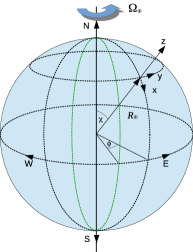
Figure 1: The position of the ILL laboratory of the qBounce experiments on the surface of the Earth.

IV Parameters of violation of Lorentz invariance in the canonical Sun–centered frame

Values of parameters of Lorentz invariance violation should in principle depend on an inertial frame, where they are measured. In the ground–based laboratory on the surface of the Earth such as the ILL, i.e.in the standard laboratory frame with coordinates $(t,x,y,z)$ (see Fig. 1), parameters of violation of Lorentz invariance should vary in time with a period ${\cal T}_{\oplus}=23\,{\rm hr}\,56\,{\rm min}\,4.09\,{\rm s}$ determined by the Earth’s sidereal angular frequency $\Omega_{\oplus}=2\pi/{\cal T}_{\oplus}=7.2921159\times 10^{-5}\,{\rm rad/s}$. It is obvious that because of rotation, yielding distinguishable inertial frames in a ground–based laboratory on the surface of the Earth, the standard laboratory frame is not appropriate for definition of the values of parameters of Lorentz invariance violation. In contrast, the frame centered on the Sun, i.e. the canonical Sun–centered frame, remains unchanged approximately inertial frame over thousands of years Kostelecky1999c –Kostelecky2016 . Thus, following Kostelecky1999c –Kostelecky2016 we define parameters of violation of Lorentz invariance in Eq.(II) in terms of the parameters of violation of Lorentz invariance in the canonical Sun–centered frame with coordinates $(T,X,Y,Z)$ (see also Smart1977 ), where $T$ is the celestial equatorial time An important point of the expression of parameters of violation of Lorentz invariance in the laboratory frame in terms of parameters in the canonical Sun–centered one we have to relate a local laboratory time $t$ to a time $T$ in the canonical Sun–centered frame, where $T$ is the celestial equatorial time Kostelecky2002b . Such a problem has been discussed in details in Kostelecky1999c –Kostelecky2016 . According to Kostelecky1999c –Kostelecky2016 , it is useful to match $t$ with the local sidereal time $T_{\oplus}$, which is measured in the canonical Sun–centered frame from one of the times when the $y$ axis lies along the $Y$ axis. The time $T{\oplus}$ is related to the celestial equatorial time $T$ by the relation Kostelecky2016

$$T_{\oplus}=T-T_{0}\quad,\quad T_{0}=\frac{66.25^{0}-\phi}{360^{0}}\,(23.934\,{\rm hr}),$$ (23)

where $\phi$ is a longitude of the laboratory measured in degrees. As the longitude of the ILL laboratory is $\phi=5.71667^{0}$, we get $T_{\oplus}=T-4\,{\rm hr}\,01\,{\rm min}\,30.44\,{\rm s}$. According to Kostelecky1999c –Kostelecky2016 , with reasonable approximation that the orbit of the Earth is circular, the transition from the canonical Sun–centered frame with coordinates $(X,Y,Z)$ to the laboratory frame with coordinates $(x,y,z)$ is given by the matrix dependent on the sidereal time $T_{\oplus}$ Kostelecky1999c –Kostelecky2016

$$R_{jJ}(T_{\oplus})=\left(\begin{array}[]{llcl}\cos\chi\cos\Omega_{\oplus}T_{\oplus}&\cos\chi\sin\Omega_{\oplus}T_{\oplus}&-\sin\chi\\ -\sin\Omega_{\oplus}T_{\oplus}&\cos\Omega_{\oplus}T_{\oplus}&0\\ \sin\chi\cos\Omega_{\oplus}T_{\oplus}&\sin\chi\sin\Omega_{\oplus}T_{\oplus}&\cos\chi\\ \end{array}\right),$$ (27)

where $j=x,y,z$ and $J=X,Y,Z$ denote the indices in the laboratory and canonical Sun–centered frames, respectively. The matrix $R(T_{\oplus})$ in Eq.(27) obeys the constraint $R(T_{\oplus})R^{T}(T_{\oplus})=R^{T}(T_{\oplus})R(T_{\oplus})=1$, where $T$ is a transposition. Now we may express parameters violating Lorentz invariance in the laboratory frame in terms of the parameters in the canonical Sun–centered frame. This concerns only parameters entering in Eq.(III.2), Eq.(20) and Eq.(22). We get

$$\bar{c}^{n}_{zz} = R_{zA}(T_{\oplus})R_{zB}(T_{\oplus})\bar{c}^{n}_{AB}=\frac{1}{2}\,\big{[}\sin^{2}\chi\big{(}\bar{c}^{n}_{XX}+\bar{c}^{n}_{YY}\big{)}+2\cos^{2}\chi\,\bar{c}^{n}_{ZZ}\big{]}+\sin\chi\cos\chi\,[\big{(}\bar{c}^{n}_{XZ}+\bar{c}^{n}_{ZX})\cos\Omega_{\oplus}T_{\oplus}$$

$$+ \big{(}\bar{c}^{n}_{YZ}+\bar{c}^{n}_{ZY}\big{)}\sin\Omega_{\oplus}T_{\oplus}\big{]}+\frac{1}{2}\,\sin^{2}\chi\big{(}\bar{c}^{n}_{XX}-\bar{c}^{n}_{YY}\big{)}\,\cos 2\Omega_{\oplus}T_{\oplus},$$

$$\bar{d}^{n}_{0z} = R_{zJ}(T_{\oplus})\bar{d}^{n}_{TJ}=\sin\chi\big{(}\bar{d}^{n}_{TX}\cos\Omega_{\oplus}T_{\oplus}+\bar{d}^{n}_{TY}\sin\Omega_{\oplus}T_{\oplus}\big{)}+\cos\chi\,\bar{d}^{n}_{TZ},$$

$$\bar{d}^{n}_{z0} = R_{zJ}(T_{\oplus})\bar{d}^{n}_{JT}=\sin\chi\big{(}\bar{d}^{n}_{XT}\cos\Omega_{\oplus}T_{\oplus}+\bar{d}^{n}_{YT}\sin\Omega_{\oplus}T_{\oplus}\big{)}+\cos\chi\,\bar{d}^{n}_{ZT},$$

$$\bar{g}^{n}_{y0z} = R_{yA}(T_{\oplus})R_{zB}(T_{\oplus})\bar{g}^{n}_{ATB}=\frac{1}{2}\,\sin\chi\,\big{(}\bar{g}^{n}_{YTX}-\bar{g}^{n}_{XTY}\big{)}+\cos\chi\,\big{(}\bar{g}^{n}_{YTZ}\,\cos\Omega_{\oplus}T_{\oplus}-\bar{g}^{n}_{XTZ}\,\sin\Omega_{\oplus}T_{\oplus}\big{)}$$

$$+ \frac{1}{2}\,\sin\chi\,\big{[}\big{(}\bar{g}^{n}_{XTY}+\bar{g}^{n}_{YTX}\big{)}\,\cos 2\Omega_{\oplus}T_{\oplus}-\big{(}\bar{g}_{XTX}-\bar{g}_{YTY}\big{)}\,\sin 2\Omega_{\oplus}T_{\oplus}\big{]},$$

$$\bar{g}^{n}_{yz0} = R_{yA}(T_{\oplus})R_{zB}(T_{\oplus})\bar{g}^{n}_{ABT}=-\sin\chi\,\bar{g}^{n}_{XYT}+\cos\chi\,\big{(}\bar{g}^{n}_{YZT}\,\cos\Omega_{\oplus}T_{\oplus}-\bar{g}^{n}_{XZT}\,\sin\Omega_{\oplus}T_{\oplus}\big{)},$$

$$\bar{g}^{n}_{x0z} = R_{xA}(T_{\oplus})R_{zB}(T_{\oplus})\bar{g}^{n}_{ATB}=\frac{1}{2}\sin\chi\cos\chi\,\big{(}\bar{g}^{n}_{XTX}+\bar{g}^{n}_{YTY}-2\bar{g}^{n}_{ZTZ}\big{)}-\big{(}\sin^{2}\chi\bar{g}^{n}_{ZTX}-\cos^{2}\chi\,\bar{g}^{n}_{XTZ}\big{)}$$

$$\times\,\cos\Omega_{\oplus}T_{\oplus}-\big{(}\sin^{2}\chi\bar{g}^{n}_{ZTY}-\cos^{2}\chi\bar{g}^{n}_{YTZ}\big{)}\sin\Omega_{\oplus}T_{\oplus}+\frac{1}{2}\,\sin\chi\cos\chi\,\big{[}\big{(}\bar{g}^{n}_{XTX}-\bar{g}^{n}_{YTY}\big{)}\,\cos 2\Omega_{\oplus}T_{\oplus}$$

$$+ \big{(}\bar{g}^{n}_{XTY}+\bar{g}^{n}_{YTX}\big{)}\sin 2\Omega_{\oplus}T_{\oplus}\big{]},$$

$$\bar{g}^{n}_{xz0} = R_{xA}(T_{\oplus})R_{zB}(T_{\oplus})\bar{g}^{n}_{ABT}=-\bar{g}^{n}_{ZXT}\,\cos\Omega_{\oplus}T_{\oplus}-\bar{g}^{n}_{ZYT}\,\sin\Omega_{\oplus}T_{\oplus},$$

$$\bar{b}^{n}_{j} = R_{jJ}(T_{\oplus})\bar{b}^{n}_{J},$$

$$\bar{d}^{n}_{j0} = R_{jJ}(t)\bar{d}^{n}_{JT},$$

$$\varepsilon_{jk\ell}\bar{g}^{n}_{kl0} = R_{jJ}(T_{\oplus})\varepsilon_{JKL}\bar{g}^{n}_{KLT},$$

$$\varepsilon_{jk\ell}\bar{H}^{n}_{k\ell} = R_{jJ}(T_{\oplus})\varepsilon_{JKL}\bar{H}^{n}_{KL}.$$ (28)

As has been pointed out in Kostelecky2002b the local sidereal time $T_{\oplus}$ should be chosen conveniently for every experiment. This can be also done defining the local sidereal time $T_{\oplus}$ in terms of the local laboratory time $t$ as follows $T_{\oplus}=t-t_{0}$, where $t_{0}$ can be determined for every run of qBounce experiments LSTime .

The transition frequencies for spin–flip and non–spin–flip transitions averaged over time impose the following upper bounds on parameters of violation of Lorentz invariance

$$|\bar{g}^{n}_{XTY}-\bar{g}^{n}_{YTX}| <\frac{2}{\sin\chi}\times 1.1\times 10^{-3}=3.1\times 10^{-3},$$

$$|\tilde{g}^{n}_{Q}| <\frac{2m}{\sin\chi\,\cos\chi}\times 1.1\times 10^{-3}=4.1\times 10^{-3}\,{\rm GeV},$$

$$|\tilde{d}^{n}_{Z}| <\frac{1}{2\,\cos\chi}\times 5.1\times 10^{-4}\,{\rm GeV}=3.6\times 10^{-4}\,{\rm GeV},$$ (29)

where we have used the notation $\tilde{g}^{n}_{Q}=m\big{(}\bar{g}^{n}_{XTX}+\bar{g}^{n}_{YTY}-2\bar{g}^{n}_{ZTZ}\big{)}$ Kostelecky1999c , and

$$\big{|}(1+\sin^{2}\chi)\,\tilde{c}^{n}_{Q}+5\,m\,\bar{c}^{n}_{ZZ}\big{|}<3.4\times 10^{-3}m,$$ (30)

where we have used the notation $\tilde{c}^{n}_{Q}=m(\bar{c}^{n}_{XX}+\bar{c}^{n}_{YY}-2\bar{c}^{n}_{ZZ})$ Kostelecky1999c and the traceless of $\bar{c}^{n}_{\mu\nu}$, i.e. $\bar{c}^{n}_{TT}=\bar{c}^{n}_{XX}+\bar{c}^{n}_{YY}+\bar{c}^{n}_{ZZ}$. Since $\tilde{c}^{n}_{Q}=(-1.8\pm 2.2)\times 10^{-14}\,{\rm GeV}$ (see Ref.Kostelecky2011b (see p.36, Table D12)), we may neglect the contribution of $\tilde{c}^{n}_{Q}$ and place a new constraint $|\bar{c}^{n}_{ZZ}|<6.8\times 10^{-4}$. We would like to emphasize that so far the parameter $|\bar{c}^{n}_{ZZ}|$ was not yet estimated (see Ref. Kostelecky2011b , p.36, Table D12). Then, using $\tilde{c}^{n}_{Q}=(-1.8\pm 2.2)\times 10^{-14}\,{\rm GeV}$ and $\bar{c}^{n}_{XX}-\bar{c}^{n}_{YY}=(1.4\pm 1.7)\times 10^{-29}$ (see Ref. Kostelecky2011b , p.36, Table D12), and $|\bar{c}^{n}_{ZZ}|<6.8\times 10^{-4}$ one may assume that $|\bar{c}^{n}_{XX}|=|\bar{c}^{n}_{YY}|<6.8\times 10^{-4}$. Using the property $\eta^{\mu\nu}\bar{c}^{n}_{\mu\nu}=0$ of the tensor $\bar{c}^{n}_{\mu\nu}$ we get $|\bar{c}^{n}_{TT}|=3|\bar{c}^{n}_{ZZ}|<2.0\times 10^{-3}$. Of course, such an estimate we can make also as follows. Expressing the parameter $m\bar{c}^{n}_{ZZ}$ in terms of $\bar{c}^{n}_{Q}$ and $m\bar{c}^{n}_{TT}$, we get $m\bar{c}^{n}_{ZZ}=(m\bar{c}^{n}_{TT}-\bar{c}^{n}_{Q})/3$ and transcribe Eq.(30) into the form

$$\Big{|}\Big{(}\sin^{2}\chi-\frac{2}{3}\Big{)}\,\bar{c}^{n}_{Q}+\frac{5}{3}\,m\,\bar{c}^{n}_{TT}\Big{|}<3.4\times 10^{-3}\,m.$$ (31)

Because of the experimental data $\tilde{c}^{n}_{Q}=(-1.8\pm 2.2)\times 10^{-14}\,{\rm GeV}$ giving $\bar{c}^{n}_{ZZ}=(\bar{c}^{n}_{XX}+\bar{c}^{n}_{YY})/2$, the experimental data $\bar{c}^{n}_{XX}-\bar{c}^{n}_{YY}=(1.4\pm 1.7)\times 10^{-29}$ giving $\bar{c}^{n}_{XX}=\bar{c}^{n}_{YY}=\bar{c}^{n}_{ZZ}$ and the relation $\bar{c}^{n}_{ZZ}=\bar{c}^{n}_{TT}/3$, we arrive at the constraint $|\bar{c}^{n}_{ZZ}|<6.8\times 10^{-4}$.

In Table I we have collected the obtained results in the form accepted in Kostelecky2011b . Of course, all of these estimates should be treated as a theoretical basis for future qBounce experiments of searches for effects of interactions violating Lorentz invariance in the neutron sector of the SME.

Combination	Result
$|\bar{c}^{n}_{XX}|$	$<6.8\times 10^{-4}$
$|\bar{c}^{n}_{YY}|$	$<6.8\times 10^{-4}$
$|\bar{c}^{n}_{ZZ}|$	$<6.8\times 10^{-4}$
$|\bar{c}^{n}_{TT}|$	$<2.0\times 10^{-3}$
$|\bar{g}^{n}_{XTY}-\bar{g}^{n}_{YTX}|$	$<3.1\times 10^{-3}$
$|\tilde{g}_{Q}|$	$<4.1\times 10^{-3}\,{\rm GeV}$
$\big{|}\tilde{d}^{n}_{Z}\big{|}$	$<3.6\times 10^{-4}\,{\rm GeV}$

Table 1: Neutron sector. A theoretical basis for an experimental analysis of upper bounds of parameters of Lorentz invariance violation in the neutron sector of the SME obtained by using the current experimental sensitivity $\Delta E<2\times 10^{-15}\,{\rm eV}$ of qBounce experiments Cronenberg2018 .

V Evolution of spin operator of UCNs

A time evolution of the spin operator $\vec{S}$ of UCNs is described by Heisenberg’s equation of motion LL1965

$$\frac{d\vec{S}}{dt}=\frac{\partial\vec{S}}{\partial t}+i\,[{\rm H},\vec{S}\,]=\frac{\partial\vec{S}}{\partial t}+i\,[\Phi_{\rm nLV},\vec{S}\,].$$ (32)

Since the spin operator $\vec{S}$ does not depend explicitly on time, the partial derivative in Eq.(20) is equal to zero. Then, using the effective non–relativistic potential Eq.(II) and the commutation relation $[S_{a},S_{b}]=i\varepsilon_{abc}S_{c}$ we get

$$\frac{d\vec{S}}{dt}=\vec{\Omega}_{\rm nLV}\times\vec{S},$$ (33)

where $\vec{\Omega}_{\rm nLV}$ is the angular velocity operator, induced by violation of Lorentz invariance. It is equal to

$$(\vec{\Omega}_{\rm nLV})_{a} = -2\tilde{b}^{n}_{a}+\Big{(}2b^{n}_{0}\delta_{ja}-2m(d^{n}_{aj}+d^{n}_{00}\delta_{aj})-m\,\varepsilon_{a\ell m}\big{(}g^{n}_{m\ell j}+2g_{m00}\delta_{j\ell}\big{)}-2\varepsilon_{ja\ell}H^{n}_{\ell 0}\Big{)}\frac{p_{j}}{m}$$ (34)

$$+ \Big{\{}\Big{(}-b^{n}_{j}+2\tilde{d}^{n}_{j}-\frac{1}{2}\,m\,\varepsilon_{jmn}\,g^{n}_{mn0}\Big{)}\delta_{ka}+b^{n}_{a}+\frac{1}{2}\,m\,\varepsilon_{amn}g^{n}_{mn0}\delta_{jk}-m\,\varepsilon_{jam}\,(g^{n}_{m0k}+g^{n}_{mk0})\Big{\}}\frac{p_{j}p_{k}}{m^{2}}.$$

Thus, Eq.(33) with the angular velocity operator Eq.(34) defines an spin evolution of UCNs caused by interactions violating Lorentz invariance. A dependence of the parameters violating Lorentz invariance on time and the Earth’s sidereal frequency leads to fluctuations of the angular velocity $\vec{\Omega}_{\rm nLV}$ with a period ${\cal T}_{\oplus}=23\,{\rm hr}\,56\,{\rm min}\,4.09\,{\rm s}$ of the Earth’s rotation.

VI Discussion

In this paper we have proposed to extract constraints on the parameters of Lorentz invariance violation from measurements of transition frequencies of transitions between quantum gravitational states of unpolarized and polarized UCNs by the qBounce Collaboration Cronenberg2018 ; Ivanov2013 . Neglecting contributions of parameters of violation of Lorentz invariance in the gravitational sector of the SME, and using the effective non–relativistic potential for interactions violating Lorentz invariance in the neutron sector of the SME, derived by Kostelecký and Lane Kostelecky1999b , we have calculated the corrections, caused by interactions violating Lorentz invariance, to transition frequencies of transitions between quantum gravitational states of unpolarized and polarized UCNs. We have carried out the calculations in the standard laboratory frame relative to the location of the ILL laboratory on the surface of the Earth.

For the extraction of constraints on parameters of violation of Lorentz invariance from these corrections it is important to define parameters of violation of Lorentz invariance relative to an inertial frame. Because of rotation of the Earth all terrestrial laboratories are non–inertial and parameters of violation of Lorentz invariance, analyzed in any terrestrial laboratory, should be expressed in terms of parameters of violation of Lorentz invariance in an inertial frame, for example, in the canonical Sun–centered frame, which remains unchanged approximately inertial frame over thousands of years Kostelecky1999c –Kostelecky2016 .

Having expressed parameters of violation of Lorentz invariance, which are responsible for corrections to the transition frequencies of transitions between quantum gravitational states of unpolarized and polarized UCNs in the ILL laboratory, in terms of parameters of violation of Lorentz invariance defined in the canonical Sun–centered frame, we have placed some new constraints (see Table I) in comparison to the results represented in Ref.Kostelecky2011b (see Ref.Kostelecky2011b , Table D12). In Table I we have adduced the constraints on parameters of violation of Lorentz invariance using the current sensitivity $\Delta E<2\times 10^{-15}\,{\rm eV}$ of the qBounce experiments Cronenberg2018 , which is closely related to experimental uncertainties of the experimental data Cronenberg2018 (see also a discussion below Eq.(18)). The results represented in Table I may serve as a theoretical basis for experimental searches of effects of violation of Lorentz invariance in the neutron sector of the SME in qBounce experiments.

Thus, following the results given in Table I one may assert that even for the current sensitivity $\Delta E<2\times 10^{-15}\,{\rm eV}$ of the qBounce experiments Cronenberg2018 the analysis of transition frequencies of transitions between quantum gravitational states of unpolarized and polarized UCNs may allow to place new constraints on parameters of violation of Lorentz invariance in the neutron sector of the SME. The qBounce experiments on an analysis of contributions of interactions violating Lorentz invariance will be carried out at Instrument PF2/UCN at ILL. A possible improvement of experimental sensitivity of the qBounce experiments up to $\Delta E<10^{-17}\,{\rm eV}$ in the nearest future and finally to reach a sensitivity $\Delta E<10^{-21}\,{\rm eV}$ Abele2010 should allow to improve substantially upper bounds of parameters in Table I. In our forthcoming publication we are planning to analyze contributions of interactions violating Lorentz invariance from the gravitational sector of the SME Kostelecky2006 ; Kostelecky2011a .

VII Acknowledgements

We are grateful to Alan Kostelecký for fruitful discussions and comments. The work of A. N. Ivanov was supported by the Austrian “Fonds zur Förderung der Wissenschaftlichen Forschung” (FWF) under the contracts P31702-N27 and P26636-N20, and “Deutsche Förderungsgemeinschaft” (DFG) AB 128/5-2. The work of M. Wellenzohn was supported by the MA 23 (FH-Call 16) under the project “Photonik - Stiftungsprofessur für Lehre”.

References

- (1) V. A. Kostelecký, Gravity, Lorentz violation, and the standard model, Phys. Rev. D 69, 105009 (2004); DOI: 10.1103/PhysRevD.69.105009.
- (2) M. Tanabashi et al. (Particle Data Group), Phys. Rev. D 98, 030001 (2018); DOI: 10.1103/PhysRevD.98.030001.
- (3) D. Colladay and V. A. Kostelecký, CPT violation and the standard model, Phys. Rev. D 55, 6760 (1997); DOI: 10.1103/PhysRevD.55.6760.
- (4) D. Colladay and V. A. Kostelecký, Lorentz violating extension of the standard model, Phys. Rev. D 58, 116002 (1998); DOI: 10.1103/PhysRevD.58.116002.
- (5) Q. G. Bailey and V. A. Kostelecký, Signals for Lorentz violation in post-Newtonian gravity, Phys. Rev. D 74, 045001 (2006); DOI: 10.1103/PhysRevD.74.045001.
- (6) V. A. Kostelecký and J. Tasson, Matter-gravity couplings and Lorentz violation, Phys. Rev. D 83, 016013 (2011); DOI: 10.1103/PhysRevD.83.016013.
- (7) R. F. Streater and A. S. Wightman, PCT, spin and statistics, and all that, Princeton University Press, Princeton and Oxford, Third printing (1980).
- (8) O. W. Greenberg, CPT violation implies violation of Lorentz invariance, Phys. Rev. Lett. 89, 231602 (2002); DOI: 10.1103/PhysRevLett.89.231602.
- (9) R. Bluhm, V. A. Kostelecký, and N. Russell, Testing CPT with anomalous magnetic moments, Phys. Rev. Lett. 79, 1432 (1997); DOI:” 10.1103/PhysRevLett.79.1432.
- (10) R. Bluhm, V. A. Kostelecký, and N. Russell, CPT and Lorentz tests in Penning traps, Phys. Rev. D 57, 3932 (1998); DOI: 10.1103/PhysRevD.57.3932.
- (11) R. Bluhm, V. A. Kostelecký, and N. Russell, CPT and Lorentz tests in hydrogen and anti-hydrogen, Phys. Rev. Lett. bf 82, 2254 (1999); DOI: 10.1103/PhysRevLett.82.2254.
- (12) V. A. Kostelecký and A. J. Vargas, Lorentz and CPT tests with hydrogen, antihydrogen, and related systems, Phys. Rev. D 92, 056002 (2015); DOI: 10.1103/PhysRevD.92.056002. YYY
- (13) R. Bluhm, V. A. Kostelecký, and Ch. D. Lane, CPT and Lorentz tests with muons, Phys. Rev. Lett. 84, 1098 (2000); DOI: 10.1103/PhysRevLett.84.1098.
- (14) A. H. Gomes, V. A. Kostelecký, and A. J. Vargas, Laboratory tests of Lorentz and CPT symmetry with muons, Phys. Rev. D 90, 076009 (2014); DOI: 10.1103/PhysRevD.90.076009.
- (15) J. S. Díaz, V. A. Kostelecký, and R. Lehnert, Relativity violations and beta decay, Phys. Rev. D 88, 071902 (2013); DOI: 10.1103/PhysRevD.88.071902.
- (16) V. A. Kostelecký and N. Russell, Data Tables for Lorentz and CPT Violation, Rev. Mod. Phys. 83, 11 (2011); DOI: 10.1103/RevModPhys.83.11; 2019 edition, arXiv: 0801.0287v12 [hep-ph].
- (17) V. V. Nesvizhevsky, H. G. Börner, A. M. Gagarsky, G. A. Petrov, A. K. Petukhov, H. Abele, S. Bäßler, T. Stoferle, and S. M. Solovev, Search for quantum states of the neutron in a gravitational field: Gravitational levels, Nucl. Instrum. Meth. A 440, 754 (2000); DOI: 10.1016/S0168-9002(99)01077-3.
- (18) V. V. Nesvizhevsky, H. G. Börner, A. K. Petukhov, H. Abele, S. Bäßler, F. J. Ruess, T. Stoferle, A. Westphal, A. M. Gagarski, G. A. Petrov, and A. V. Strelkov, Quantum states of neutrons in the Earth’s gravitational field, Nature 415, 297 (2002); DOI: 10.1038/415297a.
- (19) V. V. Nesvizhevsky, H. G. Börner, A. M. Gagarski, A. K. Petukhov, H. Abele, S. Bäßler, G. Divkovic, F. J. Ruess, T. Stoferle, A. Westphal, A. V. Strelkov, K.V. Protasov, and A. Yu. Voronin, Measurement of quantum states of neutrons in the earth’s gravitational field, Phys. Rev. D 67, 102002 (2003); DOI: 10.1103/PhysRevD.67.102002.
- (20) V. V. Nesvizhevsky, A. K. Petukhov, H. G. Börner, T. A. Baranova, A. M. Gagarski, G. A. Petrov, K. V. Protasov, A. Yu. Voronin, S. Bäßler, H. Abele, A. Westphal, and L. Lucovac, Study of the neutron quantum states in the gravity field, Eur. Phys. J. C 40, 479 (2005); DOI: 10.1140/epjc/s2005-02135-y.
- (21) H. Abele, S. Bäßler, and A. Westphal, Quantum states of neutrons in the gravitational field and limits for non-Newtonian interaction in the range between 1 micron and 10 microns, Lect. Notes Phys. 631, 355 (2003); DOI: 10.1007/978-3-540-45230-0.
- (22) V. V. Nesvizhevsky and K. V. Protasov, Constraints on non-Newtonian gravity from the experiment on neutron quantum states in the Earth’s gravitational field, Class. Quant. Grav. 21, 4557 (2004); DOI: 10.1088/0264-9381/21/19/005.
- (23) O. Bertolami and F. M. Nunes, Ultracold neutrons, quantum effects of gravity and the weak equivalence principle, Class. Quantum Grav. 20, L61 (2003); DOI: 10.1088/0264-9381/20/5/103.
- (24) Yu. N. Pokotilovski, Constraints on strongly coupled chameleon fields from the experimental test of the weak equivalence principle for the neutron, Pisma Zh. Eksp. Teor. Fiz. 96, 841 (2012), JETP Lett. 96, 751 (2013); DOI: 10.1134/S0021364012240095.
- (25) I. I. Rabi, S. Millman, P. Kusch, and J. R. Zacharias, The molecular beam resonance method for measuring nuclear magnetic moments. The magnetic moments of , and , Phys. Rev. 55, 526 (1939); DOI: 10.1103/PhysRev.55.526.
- (26) H. Abele, T. Jenke, D. Stadler, and P. Geltenbort, QuBounce: the dynamics of ultra-cold neutrons falling in the gravity potential of the Earth, Nucl. Phys. A 827, 593c (2009); DOI: 10.1016/j.nuclphysa.2009.05.131.
- (27) T. Jenke, D. Stadler, H. Abele, and P. Geltenbort, Q-BOUNCE—Experiments with quantum bouncing ultracold neutrons, Nucl. Instr. and Meth. in Physics Res. A 611, 318 (2009); DOI: 10.1016/j.nima.2009.07.073.
- (28) H. Abele, T. Jenke, H. Leeb, and J. Schmiedmayer, Ramsey’s method of separated oscillating fields and its application to gravitationally induced quantum phaseshifts, Phys. Rev. D 81, 065019 (2010); DOI: 10.1103/PhysRevD.81.065019.
- (29) T. Jenke, P. Geltenbort, H. Lemmel, and H. Abele, Realization of a gravity-resonance-spectroscopy technique, Nature Physics 7, 468 (2011); DOI: 10.1038/nphys1970.
- (30) H. Abele and H. Leeb, Gravitation and quantum interference experiments with neutrons, New J. Phys. 14, 055010 (2012); DOI: 10.1088/1367-2630/14/5/055010.
- (31) T. Jenke, G. Cronenberg, J. Bürgdorfer, L. A. Chizhova, P. Geltenbort, A. N. Ivanov, T. Lauer, T. Lins, S. Rotter, H. Saul, U. Schmidt, and H. Abele, Phys. Rev. Lett. 112, 151105 (2014); DOI: 10.1103/PhysRevLett.112.151105.
- (32) T. Jenke and H. Abele, Experiments with gravitationally-bound ultracold neutrons at the European Spallation Source ESS, Phys. Procedia 51, 67 (2014); DOI: 10.1016/j.phpro.2013.12.016.
- (33) J. Schmiedmayer and H. Abele, Probing the dark side, Science 349, 786 (2015); DOI: 10.1126/science.aac9828.
- (34) G. Cronenberg, H. Filter, M. Thalhammer, T. Jenke, H. Abele, and P. Geltenbort, A gravity of Earth measurement with a qBOUNCE experiment, PoS EPS-HEP2015 408, (2015); DOI: 10.22323/1.234.0408.
- (35) H. Abele, Precision experiments with cold and ultracold neutrons, Hyperfine Interact. 237, 155 (2016); DOI: 10.1007/s10751-016-1352-z.
- (36) G. Konrad and H. Abele, Cold and ultracold neutrons as probes of new physics, PoS INPC2016, 359 (2017); DOI: 10.22323/1.281.0359.
- (37) G. Cronenberg, Ph. Brax, H. Filter, P. Geltenbort, T. Jenke, G. Pignol, M. Pitschmann, M. Thalhammer, and H. Abele, Acoustic Rabi oscillations between gravitational quantum states and impact on symmetron dark energy, Nature Phys. 14, 1022 (2018); DOI: 10.1038/s41567-018-0205-x.
- (38) A. Martín-Ruiz and C. A. Escobar, Testing Lorentz- and CPT-invariance with ultracold neutrons, Phys. Rev. D 97, 095039 (2018); DOI: 10.1103/PhysRevD.97.095039.
- (39) C. A. Escobar and A. Martín-Ruiz, Gravitational searches for Lorentz violation with ultracold neutrons, Phys. Rev. D 99, 075032 (2019); DOI: 10.1103/PhysRevD.99.075032.
- (40) Zhi Xiao, The CPT-violating effects on neutron’s gravitational bound state, arXiv: 1906.00146 [hep-ph], arXiv: 1906.02011 [hep-ph].
- (41) J. Khoury and A. Weltman, Chameleon cosmology, Phys. Rev. D 69, 044026 (2004); DOI: 10.1103/PhysRevD.69.044026.
- (42) A. N. Ivanov, R. Höllwieser, T. Jenke, M. Wellenzohn, and H. Abele, Influence of the chameleon field potential on transition frequencies of gravitationally bound quantum states of ultracold neutrons, Phys. Rev. D 87, 105013 (2013); DOI: 10.1103/PhysRevD.87.105013.
- (43) A. N. Ivanov and M. Wellenzohn, Nonrelativistic approximation of the Dirac equation for slow fermions coupled to the chameleon and torsion fields in the gravitational field of the Earth, Phys. Rev. D 92, 065006 (2015); DOI: 10.1103/PhysRevD.92.065006.
- (44) A. N. Ivanov, G. Cronenberg, R. Höllwieser, M. Pitschmann, T. Jenke, M. Wellenzohn, and H. Abele, Exact solution for chameleon field, self-coupled through the Ratra-Peebles potential with and confined between two parallel plates, Phys. Rev. D 94, 085005 (2016); DOI: 10.1103/PhysRevD.94.085005.
- (45) M. Jaffe, Ph. Haslinger, V. Xu, P. Hamilton (UCLA), A. Upadhye, B. Elder, J. Khoury, and H. Müller, Testing sub-gravitational forces on atoms from a miniature, in-vacuum source mass, Nature Phys. 13, 938 (2017); DOI: 10.1038/nphys4189.
- (46) K. Hinterbichler and J. Khoury, Symmetron fields: Screening Long-range forces through local symmetry restoration, Phys. Rev. Lett. 104, 231301 (2010); DOI: 10.1103/PhysRevLett.104.231301.
- (47) V. A. Kostelecký and Ch. D. Lane, Nonrelativistic quantum Hamiltonian for Lorentz violation, J. Math. Phys. 40, 6245 (1999); DOI: 10.1063/1.533090.
- (48) L. D. Landau and E. M. Lifshitz, in Quantum mechanics, Non–relativistic theory, Vol. 3 of Course of Theoretical Physics, second edition, revised and enlarged, Pergamon Press, Oxford London Edinburgh New York Paris Frankfurt, 1965.
- (49) A. S. Davydov, in Quantum mechanics, Pergamon Press, Oxford London Edinburgh New York Paris Frankfurt, 1965.
- (50) C. Itzykson and J. Zuber, in Quantum Field Theory, McGraw–Hill, New York 1980.
- (51) L. L. Foldy and S. A. Wouthuysen, On the Dirac theory of spin 1/2 particle and its nonrelativistic limit, Phys. Rev. 78, 29 (1950); DOI: 10.1103/PhysRev.78.29.
- (52) R. L. Gibbs, The quantum bouncer, Am. J. Phys. 43, 25 (1975); DOI: 10.1119/1.10024.
- (53) A. Westphal, H. Abele, S. Bäßler, V. V. Nesvizhevsky, K .V. Protasov, and A. Y. Voronin, A quantum mechanical description of the experiment on the observation of gravitationally bound states, Eur. Phys. J. C51, 367(2007); DOI: 10.1140/epjc/s10052-007-0283-x.
- (54) J. R. Albright, Integrals of products of Airy functions, J. Phys. A: Math. Gen. 10, 485 (1977); DOI: 10.1088/0305-4470/10/4/011.
- (55) V. A. Kostelecký and Ch. D. Lane, Constraints on Lorentz violation from clock-comparison experiments, Phys. Rev. D 60, 116010 (1999); DOI: 10.1103/PhysRevD.60.116010.
- (56) R. Bluhm, V. A. Kostelecký, Ch. D. Lane, and N. Russell, Clock-comparison tests of Lorentz and CPT symmetry in space, Phys. Rev. Lett. 88, 090801 (2002); DOI: 10.1103/PhysRevLett.88.090801.
- (57) V. A. Kostelecký and M. Mewes, Signals for Lorentz violation in electrodynamics, Phys. Rev. D 66, 056005 (2002); DOI: 10.1103/PhysRevD.66.056005.
- (58) R. Bluhm, V. A. Kostelecký, Ch. D. Lane, and N. Russell, Probing Lorentz and CPT violation with space-based experiments, Phys. Rev. D 68, 125008 (2003); DOI: 10.1103/PhysRevD.68.125008.
- (59) V. A. Kostelecký and M. Mewes, Electrodynamics with Lorentz-violating operators of arbitrary dimension, Phys. Rev. D 80, 015020 (2009); DOI: 10.1103/PhysRevD.80.015020.
- (60) Y. Ding and V. A. Kostelecký, Lorentz-violating spinor electrodynamics and Penning traps, Phys. Rev. D 94, 056008 (2016); DOI: 10.1103/PhysRevD.94.056008.
- (61) GPS coordinates of Grenoble, France; https://latitude.to/map/fr/france/cities/grenoble
- (62) W. M. Smart, Textbook on Spherical Astronomy, sixth edition revised by R. M. Green, Cambridge University Press, Cambridge London (1977).
- (63) A definition of the local sidereal time as a function of a local laboratory time at the ILL laboratory in Grenoble. We set , where can be determined for every experimental run of qBounce experiments; http://www.jgiesen.de/astro/astroJS/siderealClock/