Introduction to nonlinear discrete systems: Theory and modeling

Abstract

An analysis of discrete systems is important for understanding of various physical processes, such as excitations in crystal lattices and molecular chains, the light propagation in waveguide arrays, and the dynamics of Bose-condensate droplets. In basic physical courses, usually linear properties of discrete systems are studied. In this paper we propose a pedagogical introduction to the theory of nonlinear distributed systems. The main ideas and methods are illustrated using a universal model for different physical applications, the discrete nonlinear Schrödinger (DNLS) equation. We consider solutions of the DNLS equation and analyze their linear stability. The notions of nonlinear plane waves, modulational instability, discrete solitons and the anti-continuum limit are introduced and thoroughly discussed. A Mathematica program is provided for better comprehension of results and further exploration. Also, few problems, extending the topic of the paper, for independent solution are given.

• 23 February 2018

Keywords: Discrete systems; Lattices, arrays, chains; Discrete nonlinear Schrödinger equation; Discrete solitons; Mathematica code

1 Introduction

A discrete system is a system that consists of several (or an infinite number of) well-separated points (sites). Each site is characterized by some variables, so that at a given time these variables specify a state of the system. A change of variables on each site may depend on values on other sites.

Many important physical systems, such as crystal lattices, atomic chains, polymers, arrays of resonators and waveguides, electrical transmission lines, and spin lattices are essentially discrete [1, 2, 3, 4, 5, 6]. A recent advance in this field is summarized in books and research papers, that are written mainly for specialists. The purpose of this paper is to give an accessible introduction to the subject, and to illustrate the analytical methods used.

Different aspects of discrete systems are discussed in educational literature (see e.g. [7, 8, 9, 10, 11]) to enhance the corresponding university courses. However, mainly linear properties are studied in such courses. In this work, the basic ideas of the nonlinear dynamics are presented. We demonstrate main steps for analysis of discrete systems, using a well-studied model, the discrete nonlinear Schrödinger (DNLS) equation [1, 2, 3, 4, 5, 6]. We analyze properties of plane waves and localized modes. We also provide a script in Mathematica that helps to do the analysis. A student can test these methods on the DNLS equation, and then extend and modify them to study more complex systems. Our paper can also be useful for lecturers, who want to include this topic to courses on nonlinear physics.

The DNLS equation is written in the following form:

$$i{du_{k}\over dt}+\beta_{0}u_{k}+\beta(u_{k+1}+u_{k-1})+\gamma|u_{k}|^{2}u_{k}=0,$$ (1)

where $u_{k}$ is the field value at $k$-th point, $k$ is an integer number, $\beta>0$ characterizes a coupling with neighbor sites, and $\gamma$ is the nonlinearity parameter. In this Section, we give examples of different physical systems described by Eq. (1).

Let us consider an array of optical waveguides, see Fig. 1(a). The field variable $u_{k}$ corresponds to the electric field $E$ in $k$-th waveguide. Waveguides are situated close to each other, so that light in one waveguide can tunnel into nearest-neighbor waveguides. This effect induces an overlap of modes and interaction of fields in the adjacent waveguides (see the third term in Eq. (1)). It is assumed that the refractive index $n$ of the material is intensity-dependent, $n=n_{0}+n_{2}|E|^{2}$. Such a dependence of $n$ results in linear (the second) term and nonlinear (the fourth) term in Eq. (1). Therefore, Eq. (1) describes light propagation in a waveguide array. The equation can be derived from the Maxwell equations in the limit of weakly coupled modes [1, 4, 6]. Parameter $\beta_{0}$ is the linear propagation constant, $\beta$ is the coupling coefficient, and $\gamma\sim n_{2}$ characterizes the Kerr nonlinearity. The propagation distance $z$ plays here the role of time. A study of beam dynamics in arrays can be useful for light routing in photonic circuits, for beam steering and switching [1, 4, 6]. Waveguide arrays can serve as a universal testbed for analysis of phenomena from solid state physics, such as Anderson localization and Bloch oscillations.

     

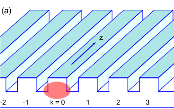
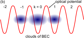
Figure 1: Examples of systems, described by the DNLS equation. (a) An array of optical rib waveguides. Light in a waveguide (a spot at $k=0$) is coupled with nearest neighbor waveguides. (b) Clouds of Bose-Einstein condensate, distributed in minima ($k=-1,0$ and 1) of the periodic optical potential.

Now, we consider a gas of ultra-cold (e.g. rubidium) atoms at temperature $\sim 10^{-7}$ K in an optical lattice, see Fig. 1(b). Because of such a low temperature, all atoms are in the ground state, and they form a new state of matter, a Bose-Einstein condensate (BEC) [12]. An optical lattice, which is a standing wave created due to interference of laser beams, forms a periodic potential for a BEC. Let us analyze a BEC distributed in the minima of the potential. A relative number of atoms in the $k$-th minimum are described by $|u_{k}|^{2}$. Then, assuming that particles on different minima interact weakly due to tunneling, and taking into account the two-body scattering effect, one can arrive to Eq. (1). More rigorous derivation of Eq. (1) from the Gross-Pitaevsky equation for a BEC in a periodic potential can be found in Ref. [13]. A BEC in optical lattices, as an ensemble of coherent objects, is actively studied from a fundamental point of view. A set of interacting condensate droplets can be used in experiments on matter wave interference, and precise measurements [12].

The DNLS Eq. (1) describes also other systems, such as Josephson junction arrays, layered magnetic systems, organic molecules and DNA, see [3, 5, 6]. Since the DNLS equation has different applications, in this work we treat it in general terms, referring to $u_{k}$ as the field variable and to $t$ as time. Now, when the physical importance of Eq. (1) is justified, let us consider its main properties.

Equation (1) has two conserved quantities

$$P=\sum_{k=1}^{N}{|u_{k}|^{2}},\quad H=\sum_{k=1}^{N}\left(\beta_{0}|u_{k}|^{2}+\beta|u_{k}-u_{k-1}|^{2}+{\gamma\over 2}|u_{k}|^{4}\right).$$ (2)

In the context of waveguide arrays, $P$ is the total power, while $H$ is the Hamiltonian. The second term in Eq. (1) can be eliminated by using transformation $u_{k}(t)\to u_{k}(t)\exp(i\beta_{0}t)$. In the rest of the paper, we assume $\beta_{0}=0$.

When $\gamma=0$, an excitation, initially localized on a single site, spreads across the array due to coupling. Nonlinearity ($\gamma\neq 0)$ can support localized states, in which the energy is locked mainly in few sites. These localized states are called discrete solitons (DSs). There are two basic types of solitons, namely, bright soltions and dark solitons. The names come from applications in optics. A bright DS corresponds to a distribution that vanishes far from the mode center. Such a mode is observed a set of bright spots located in few wavegudes. A dark DS corresponds to a dip on a constant background. We focus our attention on bright DSs.

Plane waves and DSs are considered as fundamental modes of nonlinear discrete systems. Any initial field distribution with finite $P$ ends up typically in a set of spreading waves and DSs [2, 5] . Therefore, in order to study the dynamics of discrete systems, one need to understand properties of these excitations.

2 Analysis of waves in discrete systems

2.1 Plane waves

For discrete systems, it is instructive to start the analysis from a plane wave solution. We look for a solution in the following form:

$$u_{k}(t)=a\exp[i(qk-\omega t)],$$ (3)

where $a$, $q$, and $\omega$ are the amplitude, the wave number and the frequency of the plane wave. A substitution of Eq. (3) into Eq. (1) results in the following dispersion relation:

$$\omega=-(2\beta\cos q+\gamma a^{2}).$$ (4)

This is an important characteristics of plane waves. The physical meaning of the dispersion relation is simple. If at $t=0$, one prepares a profile in a form of Eq. (3) with given $q$, then the real and imaginary parts oscillate in time with frequency $\omega$. Alternatively, exciting in time a single site with frequency $\omega$, one generates a wave with wavenumber $q$ defined by Eq. (4).

First, we consider the dispersion relation of the linear system, $\gamma=0$ (or $a\to 0$). The first derivative $d\omega/dq$ defines the group velocity, while the second derivative $d^{2}\omega/dq^{2}$ is the wave dispersion. Since, in general, $d^{2}\omega/dq^{2}\neq 0$, we conclude that the inter-site coupling induces effective dispersion. This dispersion is responsible for a spreading of initially localized distribution. Another property, worth to notice, is that dispersion can change its sign, depending on the value of $q$. We return to this property in the discussion of localized waves.

In presence of nonlinearity, $\gamma\neq 0$, the dispersion relation shifts up or down depending on sign of $\gamma$. The dependence of the wave frequency on the amplitude is typical for nonlinear systems.

For $q=0$ ($q=\pi$), amplitudes $ae^{iqk}$ in nearest-neighbor sites have the same (opposite) sign. The corresponding distribution is called unstaggered (staggered).

The next step of the analysis is to study the dynamics of small perturbations of the plane wave. A growth of small perturbations is a manifestation of modulational instability (MI). Usually, the result of MI is a structure with well-separated localized waves that can be associated with DSs.

In order to find unstable wave parameters, we represent the solution in the following form:

$$u_{k}(t)=[a+b_{k}(t)]\exp[i(qk-\omega t)],$$ (5)

where $b_{k}(t)$ is a complex amplitude of small modulations of the plane wave. Substituting Eq. (5) into Eq. (1), and taking only first-order terms on $b_{k}$, we get the following linear equation for perturbations:

$$i{db_{k}\over dt}+\omega b_{k}+\beta(b_{k-1}e^{-iq}+b_{k+1}e^{iq})+\gamma(2a^{2}b_{k}+a^{2}b_{k}^{*})=0,$$ (6)

Separating the real and imaginary parts of $b_{k}$, and representing them $\sim\exp[i(Qn-\Omega t)]$, we obtain a linear algebraic system. The compatibility condition of this system gives the dispersion relation of perturbations, cf. [5]:

$$(\Omega-2\beta\sin Q\sin q)^{2}=8\beta\sin^{2}(Q/2)\cos q\,[2\beta\sin^{2}(Q/2)\cos q-\gamma a^{2}].$$ (7)

When the right hand side of Eq. (7) is negative, $\Omega$ is complex, and plane wave (3) is unstable.

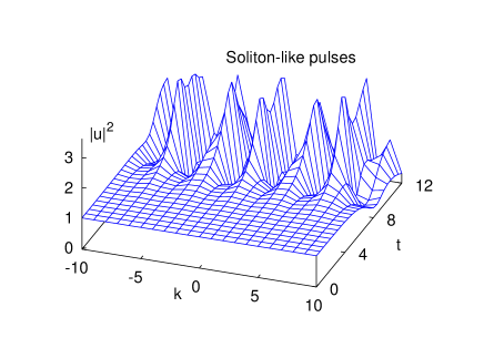
Figure 2: The dynamics of a plane wave with random modulations. The plane wave breaks up due to MI into a set of soliton-like pulses.

Figure 2 shows the dynamics of a plane wave, modulated initially by noise, $u_{k}(0)=1+\epsilon r_{k}$ , where $r_{k}$ is a random number with uniform distribution in $[-1,1]$, and $\epsilon=10^{-3}$. Numerical simulations, as in Fig. 2, can be obtained by commands, similar to those in steps 1 and 4 (MC.1 and MC.4 [14]) of the Mathematica code in A, see also Problem 1 in Sec. 3.

Since noise has waves with arbitrary $Q$, some of modulation wavenumbers are in the unstable region. As a result of instability, a plane wave breaks into a set of soliton-like pulses. Though amplitudes of pulses in Fig. 2 are varied, shapes and positions remain basically the same. Therefore, MI indicates a presence of DSs in the system. We analyze stationary DSs in the next Section.

2.2 Discrete bright solitons

There is no exact DS solutions of the DNLS equation. One can construct approximate solutions for different limiting cases. One limit is the case when the soliton width is much larger than the distance between sites. In other words, the variation of $u_{n}$ from one site to other is small. Then Eq. (1) can be approximated by the continuous NLS equation:

$$i{\partial w\over\partial t}+2\beta h^{2}{\partial^{2}w\over\partial x^{2}}+\gamma|w|^{2}w=0,$$ (8)

where $w(x_{k},t)\approx u_{k}(t)\exp(-2\beta t)$, and $h$ is the distance between neighbor sites. The NLS equation is the completely integrable model [2] that has a vast number of exact solutions. We can use the soliton solution of the NLS equation in order to construct an approximate expression for the DS:

$$u_{k,s}(t)=A\,\mbox{sech}(k/\nu)e^{i(2\beta+\gamma A^{2}/2)t},$$ (9)

where $\nu=(2\beta)^{1/2}/(A\gamma^{1/2})$ is the soliton width, and $A$ is a free parameter taken such that $\nu\gg 1$. In general, in the analysis of a discrete system, it is useful to consider the properties of its continuous counterpart.

We mention that the continuous equation (8) has bright soliton solutions when $\beta\gamma>0$ [1, 2]. In contrast, the discrete counterpart (1) can have bright solitons for any sign of $\beta\gamma$, provided that $d^{2}\omega/dq^{2}\,\gamma>0$. This is due to the change of the dispersion sign, mentioned in Sec. 2.1.

Another limit for an approximate solution is the anti-continuum limit [5], when $\beta=0$. In this case, the points are decoupled from each other. Therefore, one can write a strongly localized solution with only a single excited site

$$u_{k}(t)=A\,\delta_{0,k}\,e^{i\gamma A^{2}t}.$$ (10)

When $\beta\neq 0$, this solution is not valid, but it can be used as a basis solution in the perturbation theory or numerical simulations.

An exact profile of a DS for an arbitrary set of the system parameters can be found numerically. We look for the solution in the form $u_{k}(t)=U_{k}\exp(-i\eta t)$. Then, the soliton profile $U_{n}$ and the corresponding frequency $\eta$ are found from the nonlinear eigenvalue problem:

$$-\beta(U_{k+1}+U_{k-1})-\gamma|U_{k}|^{2}U_{k}=\eta U_{k},$$ (11)

where $k=1,\dots,N$. The derivation of this stationary equation can be checked by using symbolic calculations, see MC.2.

Eigenvalue problem (11) has $N$ equations for $N+1$ unknowns, namely, $\eta$ and $U_{1},\dots,U_{N}$, subject to vanishing (zero or periodic) boundary conditions for $U_{k}$. A direct numerical solution of such a problem is a difficult task. However, if we fix the value of $\eta$, then Eqs. (11) are just a set of $N$ nonlinear algebraic equations for $N$ unknowns. This set can easily be solved by corresponding routines, see MC.3.

For convergence of numerical solution of Eqs. (11), proper $\eta$ and an initial distribution should be chosen. A value of $\eta$ should be taken below the band of linear waves $\omega_{\mathrm{lin}}=[-2\beta,2\beta]$. This can be deduced from the analysis of the dispersion relation (4), see also Problem 4 in Sec. 3. An initial distribution can be taken in a form close to a DS, for example, $U_{k}=A\,\exp(-|k|)$, where $A$ is the soliton amplitude. An initial value of $A$ can be taken as $A=(|\eta|/\gamma)^{1/2}$, cf. Eq. (10). However, we find that the numerical procedure converges to the on-site (inter-site) soliton, even when initially only one (two) site(s) is (are) excited. Thus, in the code, different solitons can be obtained by changing parameters $\eta$, $c_{1}$ and $c_{2}$, see MC.1 and MC.3. Having a solution for one $\eta$, one can restore the whole family of soliton solutions, by changing gradually the value of $\eta$, see also Problem 6 in Sec. 3.

In order to solve the set of Eqs. (11) for a given $\eta$, one can use the Newton-Raphson method, see e.g. [15], which is the default method of the Mathematica FindRoot[] command, see MC.3. One can write Eqs. (11) in a vector form $\mathbf{f}(\mathbf{z})=0$, where $\mathbf{z}=(U_{1},U_{2},\dots,U_{N})$, and $\mathbf{f}$ is vector of functions, $\mathbf{f}=(f_{1},f_{2},\dots,f_{N})$. Then in the Newton-Raphson method, a root is found by iterations [15] $\mathbf{z}_{\mathrm{new}}=\mathbf{z}_{\mathrm{old}}+\delta\mathbf{z}$, where $\delta\mathbf{z}$ is a solution of a set of linear equations $\mathbf{J}(\mathbf{z}_{\mathrm{old}})\,\delta\mathbf{z}=-\mathbf{f}(\mathbf{z}_{\mathrm{old}})$, and $\mathbf{J}$ is the Jacobian matrix $J_{nm}=\partial f_{n}/\partial U_{m}$.

There are different types of discrete soliton solutions [1, 3, 5, 6, 16]. The distribution with a center at a site is called the on-site soliton, while that with a center between sites is called the inter-site soliton [1, 5]. Both on-site solitons and inter-site solitons can be symmetric or anti-symmetric [16]. If we define $u_{k}=(-1)^{k}v_{k}$, and change $\gamma\to-\gamma$ and $t\to-t$, then dynamics of $v_{k}(t)$ is described by the same DNLS equation. It means, in particular, that if $U_{k}$ is an unstaggered mode with frequency $\eta<0$ for $\gamma>0$, then $(-1)^{k}U_{k}$ is a staggered mode with $\eta>0$ for $\gamma<0$ [17]. This is similar to plane wave profiles with $q=0$ and $q=\pi$, respectively. We consider only unstaggered symmetric solitons for $\gamma>0$ (but see also Problem 5 in Sec. 3).

    

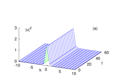
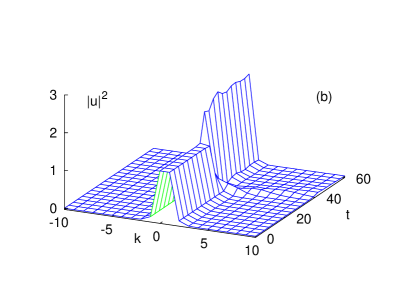
Figure 3: Dynamics of (a) on-site and (b) inter-site discrete solitons, obtained from numerical simulations of Eq. (1). The system parameters are $\beta=0.5$, $\gamma=1$, and $\eta=-2$.

We can check numerically that the solution found is indeed the eigenmode. For this purpose, we integrate numerically Eq. (1) taking the solution of Eqs. (11) as the initial condition, see MC.4. We expect a stationary evolution at least for small $t$. Such numerical simulations, using MC.4, show that on-site solitons are stable, while inter-site are unstable [1, 5]. Figure 3 shows the dynamics of stable and unstable solitons.

Physically relevant localized waves correspond to stable solutions. Therefore, it is necessary to analyze the stability of DSs. For this purpose, similarly to Eq. (5), we represent the solution as the soliton with small perturbations $w_{k}(t)$ added:

$$u_{k}(t)=[U_{k}+w_{k}(t)]\exp(-i\eta t).$$ (12)

Then, in the first approximation, the evolution of perturbations is described by the following equation:

$$i{dw_{k}\over dt}+\eta w_{k}+\beta(w_{k+1}+w_{k-1})+\gamma U_{k}^{2}(2w_{k}+w_{k}^{*})=0,$$ (13)

which can be checked with the code, see MC.5. Next, we apply a procedure similar to that used for the analysis of plane waves. Namely, we obtain from Eq. (13) the equations for the real and imaginary parts of $w_{n}$. Then substituting these parts in the form $\sim\exp(-i\Omega t)$, we get a set of linear algebraic equations in a form $\mathbf{F\,A}=\Omega\mathbf{A}$, where $\mathbf{A}$ is a real vector of length $2N$ of modulation amplitudes, and $\mathbf{F}$ is the matrix of coefficients. Eigenvalues of $\mathbf{F}$ are the frequencies of modulations. A complex frequency of modulations means instability of DSs. This stability analysis is valid also for an infinite array, $N\to\infty$. All the steps described are implemented in the code, see MC.6-MC.9. The distribution of eigenvalues on the complex $\Omega$-plane are shown in Fig. 4. Figure 4(a) shows that numerical accuracy of eigenvalue calculations is of order $10^{-7}$.

Figure 4: The distribution of modulation eigenvalues of the (a) on-site DS, and (b) inter-site DS on the complex plane of $\Omega$. The parameters are the same as in Fig. 3.

After identification of regions of stable DSs, one can perform a further study of the discrete system. For example, one can study the evolution of arbitrary localized distributions, or the interaction of discrete solitons.

3 Questions and Problems

In this Section, we suggest few problems. The aim of the problems is to help a deeper understanding of the methods reviewed in this paper, and also to develop skills in working with Mathematica program in A. Problems 1-7 consider the fundamental properties of plane waves and solitons. These properties are common for various systems. Solving these problems provides more insight into the nonlinear dynamics of discrete systems. Problems 8-12 and their extensions can be used as independent student projects. The references at each problem are sources for further study.

Problem 1 [5, 18]. Modify the program for the case of a nonlinear plane wave to obtain a plot of modulational instability similar to Fig. 2.

Problem 2 [1, 5]. The MI theory (see Eq. (7)) predicts an infinite growth of perturbations for some parameters. Does such infinite growth occur in numerical simulations of the DNLS equation?

Problem 3 [1, 5]. Prove analytically that $P$ and $H$ in Eq. (2) are indeed the invariants of Eq. (1). Include to the program a calculation of $P$. This helps to monitor errors of numerical simulations, see MC.4.

Problem 4 [1, 5]. Analyze the dispersion relation (4), and figure out why the soliton frequency should satisfy $\eta<-2\beta$ ($\beta>0$). Hint: Consider the soliton center and tails as parts of plane waves.

Problem 5 [4, 16, 17]. Find anti-symmetric on-site and inter-site solitons for $\gamma>0$. Find staggered solions for $\gamma<0$. Analyze their stability. For convergence, modify MC.3 to excite initially 3-5 consecutive sites.

Problem 6 [1, 5]. Using MC.1 and MC.3 of the program, find the dependencies of the soliton amplitude and $P$ on $\eta$.

Problem 7 [19]. An initial condition in a form of a localized mode (see Eq. (11) and MC.3) multiplied by $\exp(ipk)$, where $p$ is a constant, results in moving solitons. Modify step MC.4 of the program to generate such solitons. How does the soliton velocity depend on $\eta$ and $p$?

Problem 8 [20]. Consider a linear array with a nonlinear defect, described by the following equation

$$i{du_{k}\over dt}+\beta(u_{k+1}+u_{k-1})+\gamma\delta_{k,0}|u_{k}|^{d}u_{k}=0.$$ (14)

where $d$ is an arbitrary exponent. Find modes localized on the defect, and check their dynamics and stability.

Problem 9 [21]. Consider a semi-infinite array of waveguides, described by Eq. (1) with $k>0$ and $u_{0}=0$. Find and analyze localized modes with maximum at different distances from the border ($k=1$).

Problem 10 [22, 23]. Consider the cubic-quintic DNLS (C-Q DNLS) equation, which can be represented in the following form

$$i{du_{k}\over dt}+\beta(u_{k+1}+u_{k-1})+\gamma|u_{k}|^{2}u_{k}+\delta|u_{k}|^{4}u_{k}=0.$$ (15)

Modify and apply the program to find the different types of a localized solutions of C-Q DNLS equation and analyze their linear stability properties.

Problem 11 [2, 24, 25]. Consider the Ablowitz-Ladik (A-L) equation

$$i{du_{k}\over dt}+\beta(u_{k+1}+u_{k-1})+\gamma|u_{k}|^{2}(u_{k+1}+u_{k-1})=0.$$ (16)

This equation is an integrable discretization of the NLS equation and also has some applications in physics. It has exact solitonic solutions. Modify and apply the program to analyze the localized solutions of the A-L equation. One can include the on-site cubic term to A-L equation (which destroys the integrability) and analyze the properties of localized solutions

$$i{du_{k}\over dt}+\beta(u_{k+1}+u_{k-1})+\gamma|u_{k}|^{2}(u_{k+1}+u_{k-1})+\delta|u_{k}|^{2}u_{k}=0.$$ (17)

This equation is called the Salerno equation.

Problem 12 [26]. The following inhomogeneous DNLS equation describes the nonlinear localized impurity modes

$$i{du_{k}\over dt}+\beta(u_{k+1}+u_{k-1})+\gamma|u_{k}|^{2}u_{k}+\kappa\delta_{k,0}|u_{k}|^{4}u_{k}=0.$$ (18)

Use the Mathematica code to find these modes and check their stability.

4 Conclusion

The basic steps in the study of discrete systems have been presented. These steps include the construction of plane wave solutions and soliton solutions of the discrete system, the derivation of equations for small modulations, and analysis of stability. The corresponding code is implemented in Mathematica. It is demonstrated that theoretical consideration together with numerical modeling can substantially enhance the understanding of properties of discrete systems. The approach described here is quite generic, and it can be used to study other discrete systems.

The DNLS equation considered does not include many effects. An actual distributed system can be described by more general types of discrete equations, some examples are considered in Sec. 3. Further extension of the DNLS model includes a consideration of two- and three-dimensional arrays. Also, one can study higher-order interactions, non-local effects, and different types of nonlinearity. One can take into account external and parametric perturbations. We believe that the method and the code presented in this work can serve as a starting point to study these systems.

Appendix A Mathematica code

Here we describe a code in Mathematica (ver.8.0) for symbolic and numerical analysis of Eq. (1). A Supplementary File (both in np- and pdf-formats) provides the code with outputs, so that it gives a working example for a particular set of parameters. The code is valid for equations with nearest neighbor terms, however it can easily be extended to more general cases. Steps MC.1-MC.4 show a finding of a localized mode and a numerical simulation of its dynamics, while MC.5-MC.10 are related to a derivation of equations for modulations and calculation of the modulation spectrum.

1. Define parameters and the DNLS equation (eqn):

nPoints=200; tend=50;
par1= {$\beta$-> 0.5, $\gamma$-> 1, $\omega$-> -2}; par2= {c1-> 1., c2-> 1.};
eqn= I*u[k]’[t] + $\beta$*(u[k+1][t]+u[k-1][t]) + $\gamma$*(u[k][t])^∧2*Conjugate[u[k][t]]

2. Derive the stationary equation (eqnStat) from the DNLS equation :

sub1= u[k_ ]-> Function[{t}, U[k]*Exp[-I*$\omega$*t]];
eqn1= Simplify[eqn /.sub1, Assumptions-> {{$\omega$, t, U[i_ ]} $\in$ Reals}];
eqnStat= Coefficient[eqn1, Exp[-I*$\omega$*t]]

3. Find eigenmode (eigenMode) from the list of stationary equations (eqnStatList):

eqnStatList= Table[eqnStat, {k,1,nPoints}] /.
{U[0]-> U[nPoints], U[nPoints+1]-> U[1]};
init= Table[{U[k], (c1*KroneckerDelta[nPoints/2,k] +
c2*KroneckerDelta[nPoints/2+1,k]) /.par2}, {k,1,nPoints}];
eigenMode= FindRoot[(eqnStatList /.par1)==0, init];
init1= Table[U[k], {k,1,nPoints}] /.eigenMode;
ListLinePlot[init1, PlotRange-> {{nPoints/2-10, nPoints/2+10}, All},
PlotMarkers-> Automatic]

4. Solve the DNLSE, using eigenmode as an initial condition:

initialCond= Table[u[k][0]==init1[[k]], {k,1,nPoints}];
dnlsList= Join[Table[(eqn /.par1)==0, {k,1,nPoints}] /.
{u[0][t]-> u[nPoints][t], u[nPoints+1][t]-> u[1][t]}, initialCond];
sol1= NDSolve[dnlsList, Table[u[k], {k,1,nPoints}],
{t, 0, tend}, MaxSteps-> 1000000];
fig1= Evaluate[Table[Abs[u[k][t]], {t, 0, tend}, {k,1,nPoints}] /.sol1];
ListPlot3D[fig1, PlotRange-> All]

5. Derive an equation for the first correction, w[i][t] :

sub1= u[k_ ]-> Function[{t}, (U[k] + $\epsilon$*w[k][t]) Exp[-I*$\omega$*t]];
res1= Coefficient[Simplify[eqn /.sub1, Assumptions->
{{$\omega$, t, U[i_ ], $\epsilon$} $\in$ Reals, w[i_ ][t] $\in$ Complexes}], Exp[-I*$\omega$*t]];
eqnFirstCorr= Coefficient[Collect[res1, $\epsilon$], $\epsilon$, 1]

6. Split equation eqnFirstCorr into real and imaginary parts (wr, wi):

res1= Simplify[eqnFirstCorr /.w[k_ ] -> Function[{t}, (wr[k][t]+I*wi[k][t])],
Assumptions-> {wr[k_ ][t] $\in$ Reals, wi[k_ ][t] $\in$ Reals}];
eqnz1r= Simplify[ComplexExpand[Im[res1]]]
eqnz1i= Simplify[ComplexExpand[Re[res1]]]

7. Find left-hand sides (lhs1r and lhs1i) of the equations for spatial distributions:

sub2= {wr[k_ ]-> Function[{t}, ar[k]*Exp[-I*$\Omega$*t]],
wi[k_ ]-> Function[{t}, ai[k]*Exp[-I*$\Omega$*t]]};
eqn1r= Expand[Coefficient[Simplify[eqnz1r /.sub2], Exp[-I*$\Omega$*t], 1]];
eqn1i= Expand[Coefficient[Simplify[eqnz1i /.sub2], Exp[-I*$\Omega$*t], 1]];
lhs1r= Simplify[$\Omega$*ar[k] - eqn1r/Coefficient[eqn1r, $\Omega$*ar[k], 1]]
lhs1i= Simplify[$\Omega$*ai[k] - eqn1i/Coefficient[eqn1i, $\Omega$*ai[k], 1]]

8. Construct a matrix of coefficients in a difference form (matrF) and a vector of unknowns (vectA):

sub3= {ai[0]-> ai[nPoints], ai[nPoints+1]-> ai[1],
ar[0]-> ar[nPoints], ar[nPoints+1]-> ar[1]};
matrFdiff= Join[Table[lhs1r,{k,1,nPoints}] /.sub3,
Table[lhs1i, {k,1,nPoints}] /.sub3];
vectA= Join[Table[ar[k], {k,1,nPoints}], Table[ai[k], {k,1,nPoints}]];

9. Substitute eigenmode and parameters into matrFdiff, and convert it to a “standard” form. Then find eigenvalues of matrix F:

m1= matrFdiff /.eigenMode /.par1;
{bb1, matrF}= CoefficientArrays[m1, vectA];
ev1= Eigenvalues[Normal[matrF]]; Max[Im[ev1]]

10. Plot eigenvalues on the complex plane:

ev1Fig= Table[{Re[ev1[[i]]], Im[ev1[[i]]]}, {i,1,2*nPoints}];
ListPlot[ev1Fig, PlotRange-> All, PlotMarkers->
Graphics[{Blue,Thick,Circle[]}, ImageSize-> 8]]

References

- [1] Kivshar Yu S and Agrawal G P 2003 Optical Solitons: From Fibers to Photonic Crystals (Academic Press)
- [2] Ablowitz M J, Prinari B and Trubatch A D 2004 Discrete and Continuous Nonlinear Schrödinger Systems (Cambridge Univ. Press)
- [3] Flach S and Gorbach A V 2008 Discrete breathers - Advances in theory and applications Phys. Rep. 467 1-116
- [4] Lederer F, Stegeman G I, Christodoulides D N, Assanto G, Segev M and Silberberg Ya 2008 Discrete solitons in optics, Phys. Rep. 463 1-126
- [5] Kevrekidis P G 2009 The Discrete Nonlinear Schrödinger Equation: Mathematical Analysis, Numerical Computations and Physical Perspectives (Springer)
- [6] Kartashov Ya V, Malomed B A and Torner L 2011 Solitons in nonlinear lattices Rev. Mod. Phys. 83 247
- [7] Dauxois T, Peyrard M and Ruffo S 2005 The Fermi-Pasta-Ulam numerical experiment: history and pedagogical perspectives Eur. J. Phys. 26 S3
- [8] Lévesque L 2006 Revisiting the coupled-mass system and analogy with a simple band gap structure Eur. J. Phys. 27 133
- [9] Zhang J M and Dong R X 2010 Exact diagonalization: the Bose-Hubbard model as an example Eur. J. Phys. 31 591
- [10] Newman M E J 2011 Resource Letter CS 1: Complex Systems Am. J. Phys. 79 800
- [11] Liang C et al 2015 An undergraduate experiment of wave motion using a coupled-pendulum chain Am. J. Phys. 83 389
- [12] Pethick C J and Smith H 2008 Bose-Einstein Condensation in Dilute Gases 2nd ed. (Cambridge Univ. Press)
- [13] Trombettoni A and Smerzi A 2001 Discrete solitons and breathers with dilute Bose-Einstein condensates Phys. Rev. Lett. 86 2353
- [14] In the text, for brevity we use notation “MC.” that refers to -th step of the Mathematica code in Appendix.
- [15] Press W H, Teukolsky S A, Vetterling W T and Flannery B P 1997 Numerical Recipes in Fortran 77: the Art of Scientific Computing (Cambridge Univ. Press)
- [16] Lederer F, Darmanyan S and Kobyakov A 2001 Discrete solitons in nonlinear waveguide arrays Nonlinearity and Disorder: Theory and Applications, Abdullaev F Kh, Bang O and Sørensen M P (eds) (Kluwer Acad. Publ.)
- [17] Cai D, Bishop A R and Grønbech-Jensen N 1994 Localized states in discrete nonlinear Schrödinger (DNLS) equations Phys. Rev. Lett. 72 591
- [18] Kivshar Yu S and Peyrard M 1992 Modulational instabilities in discrete lattices Phys. Rev. A 46 3198
- [19] Kivshar Yu S and Campbell D K 1993 Peierls-Nabarro potential barrier for highly localized nonlinear modes Phys. Rev. E 48 3077
- [20] Tsironis G P, Molina M I and Hennig D 1994 Generalized nonlinear impurity in a linear chain Phys. Rev. E 50 2365
- [21] Molina M I, Vicencio R A and Kivshar Yu S 2006 Discrete solitons and nonlinear surface modes in semi-infinite waveguide arrays Opt. Lett. 31 1693
- [22] Carretero-González R, Talley J D, Chong C and Malomed B A 2006 Multistable solitons in the cubic-quintic discrete nonlinear Schrödinger equation Physica D 216 77
- [23] Abdullaev F Kh, Bouketir A, Messikh A and Umarov B A 2007 Modulational instability and discrete breathers in the discrete cubic-quintic nonlinear Shrödinger equation Physica D 232 54
- [24] Salerno M 1992 Quantum deformations of the discrete nonlinear Schrödinger equation Phys. Rev. A 46 6856
- [25] Gómez-Gardeñes J, Malomed B A, Floria L M and Bishop A R 2006 Solitons in the Salerno model with competing nonlinearities Phys. Rev. E 73 036608
- [26] Kevrekidis P G, Kivshar Yu S and Kovalev A S 2003 Instabilities and bifurcations of nonlinear impurity modes Phys. Rev. E 67 046604