Exact BER Performance Analysis for Downlink NOMA Systems Over Nakagami-$m$ Fading Channels

Abstract

In this paper, the performance of a promising technology for the next generation wireless communications, non- orthogonal multiple access (NOMA), is investigated. In particular, the bit error rate (BER) performance of downlink NOMA systems over Nakagami-$m$ flat fading channels, is presented. Under various conditions and scenarios, the exact BER of downlink NOMA systems considering successive interference cancellation (SIC) is derived. The transmitted signals are randomly generated from quadrature phase shift keying (QPSK) and two NOMA systems are considered; two users’ and three users’ systems. The obtained BER expressions are then used to evaluate the optimal power allocation for two different objectives, achieving fairness and minimizing average BER. The two objectives can be used in a variety of applications such as satellite applications with constrained transmitted power. Numerical results and Monte Carlo simulations perfectly match with the derived BER analytical results and provide valuable insight into the advantages of optimal power allocation which show the full potential of downlink NOMA systems.

$\boldsymbol{Index}$ $\boldsymbol{Terms:}$ NOMA, BER, SIC, Optimal Power Allocation, Fairness, Minimum Average BER, Nakagami-$m$.

I Introduction

The expeditious development of the mobile Internet and Internet of Things (IoT) has obtruded several challenges on the Fifth Generation (5G) and Beyond 5G (B5G) wireless communications systems. Such challenges include capacity increase by a factor of $1000$, data rates exceeding $10$ Gb/s, $10$ years battery life for machine-to-machine (M2M) communications, and network latency less than $1$ ms [1]. Consequently, extensive research has been focused in the last few years to develop the enabling technologies that can satisfy such requirements, which include dense heterogeneous networks, full-duplex communication, energy-aware communication and energy harvesting [2, 3], cloud-based radio access networks [4], wireless network virtualization [5], advanced antenna systems [6], and efficient error correction coding [7]. Moreover, great advancements have been achieved in terms of multiple access technologies such as the non-orthogonal multiple access (NOMA), which may improve the spectral efficiency and latency with respect to orthogonal multiple access (OMA) [8]. Several NOMA schemes have been actively investigated, which can be categorized into two main categories, power-domain NOMA, [9]-[10] and code-domain NOMA [11]-[12]. The focus of this paper is on the power-domain NOMA.

The performance of NOMA systems has attracted extensive literature, which is mainly focus outage probability and capacity. For example, the outage achievable rate region is studied in [13], where the results imply that NOMA outperforms OMA under similar conditions. In [14], the authors investigate a two-users NOMA system in terms of their power allocation, through the maximization of the ergodic sum capacity with the constraint of minimum sum rate requirement, fixed total transmit power, and partial channel state information (CSI) availability. In [15], a novel NOMA clustering scheme using a power allocation mechanism is presented to reduce the computational complexity at the expense of user fairness compared to the full search method. In [16], with the objective of providing proportional fairness, optimal power allocation and user pairing problems in multiuser downlink NOMA are investigated. A sum rate comparison between multiple-input multiple-output (MIMO) NOMA and OMA clusters is conducted in [17], where each cluster consists of two users. In [18], various user scheduling strategies are presented to accomplish flexible and efficient trade-offs between capacity and user fairness in NOMA systems. In [19] and [20], user clustering and power allocation for downlink NOMA system have been studied thoroughly.

More recently, noticeable efforts have focused on evaluating the bit error rate (BER) performance of NOMA systems with imperfect successive interference cancellation (SIC). For example, the authors of [21] derived closed-form expressions for the union bound on the BER of downlink NOMA with imperfect SIC over Nakagami-$m$ fading channels. Although the derived bounds are useful to estimate the BER, the results presented in [21] show that the bounds may deviate significantly from the simulation results in certain scenarios. The average BER performance of a NOMA system using space-shift keying (SSK) in Rayleigh fading channels is investigated in [22] where the exact BER is expressed in closed-form only for users two and three in a three users scenario. The exact symbol error rate (SER) for a downlink NOMA with imperfect SIC is presented in [23]. Nevertheless, using the BER is more informative when comparing different systems with different modulation orders, and the results are limited only to the two users scenario and Rayleigh fading channels. The exact SER for the two users scenario in Rayleigh fading channels is also investigated in [24]. The BER of uplink NOMA for the two users scenario is considered in [25] under imperfect SIC scenarios. The main limitation of this work is that the channel fading is considered constant over the transmission block, and hence, the channel becomes effectively an additive white Gaussian noise (AWGN) channel. An asynchronous uplink NOMA system based on triangle-SIC error is presented in [26]. Similar to [25], the channel coefficients are assumed to be fixed, hence the derived closed-form expressions can not be used in random fading scenarios. In [27], the BER is derived for a two users downlink and uplink NOMA systems over Rayleigh fading channels. However, the assumption that the links in downlink NOMA follows independent and identically distributed (i.i.d.) Rayleigh fading overlooks the large scale fading factor, which limits the contribution of this work. Moreover, the paper lacks in-depth insights into the analysis of the obtained BER results.

I-A Motivation and Main contributions

As can be noted from the aforementioned literature survey, to the best of the authors’ knowledge, there is no work reported that considers the exact BER analysis of downlink NOMA in Nakagami-$m$ fading channels. Moreover, the works considered the special case where $m=1$, i.e. Rayleigh, focus on the two-users scenario. Therefore, the main contributions of this paper are summarized as follows:

1. The exact BER performance analysis of a downlink NOMA with imperfect SIC over Nakagami-$m$ flat fading channel is considered, where exact analytical BER expressions are derived for each user individually for the cases of two and three users’ scenarios. The derived BER expressions are verified by Monte Carlo simulations.

2. The exact BER is derived in terms of a closed-form expressions for the special case of $m=1$, Rayleigh fading, for two and three users scenarios.

3. The optimal power allocation for all users is investigated based on the derived BER expressions for two different criteria. In the first, the power allocation for each user is allocated optimally to guarantee fairness among all users, which is expressed in terms of equal BER for all users. In the second, the power allocation coefficients are selected optimally to minimize the average BER for all users.

I-B Notations

To notations used throughout the paper are as follows. $\Pr(\cdot)=\mathrm{P\!}\left(\cdot\right)$, $\mathrm{P}\left(a,b\right)=\mathrm{P\!}\left(a\cap b\right)$, $\mathrm{P\!}\left(a;b\right)=\mathrm{P\!}\left(a\cup b\right)$, $\mathrm{P\!}\left(s_{1}=a_{c},s_{2}=a_{k},s_{3}=a_{v}\right)$ $\rightarrow$ $\mathrm{P\!}\left(a_{c},a_{k},a_{v}\right)$, $P_{b_{ni}}\triangleq\mathrm{P\!}\left(\hat{b}_{ni}\neq b_{ni}\right)$, $b_{ni}=c\rightarrow b_{ni}^{(c)}$, $c\in\left\{0,1\right\}$, and $s_{n}=a_{i}\rightarrow s_{n}^{(i)}$, $i\in\left\{0,1,2,3\right\}$.

I-C Paper organization

The rest of the paper is organized as follows. In Sec. II, the system and channel models are presented. This is followed by exact BER analysis for the two-users and three-users downlink NOMA systems are presented in Sec. III and Sec. IV, respectively. The optimal power allocation problem is formulated in Sec. V, while numerical and simulation results are shown in Sec. VI. Finally, the work is concluded in Sec. VII.

II System and Channel Models

This work considers a power-domain downlink NOMA system with $N$ users, $U_{1}$, $U_{2}$, $\ldots$, $U_{N}$. The users’ equipment (UEs) and the base station (BS) are equipped with single antennas [21]. Therefore, the transmitted signal from the BS can be expressed as

$$x=\mathop{\displaystyle\sum}\limits_{n=1}^{N}\sqrt{\beta_{n}P_{T}}s_{n}$$ (1)

where $s_{n}$ is the information signal of the $n$th user selected uniformly from a particular symbol constellation, $P_{T}$ is the BS transmit power, and $\beta_{n}$ is the allocated power coefficient for the $n$th user such that $\mathop{\displaystyle\sum}_{n=1}^{N}\beta_{n}=1$. For the rest of the paper, the transmit power $P_{T}$ is normalized to unity.

In flat fading channels, the received signal at the $n$th UE can be written as

$$r_{n}=h_{n}x+w_{n}$$ (2)

where $h_{n}$ represents the link between the BS and the $n$th user whose probability density function (PDF) is described in Appendix I and $w_{n}$ is the AWGN, $w_{n}\sim\mathcal{CN}\left(0,N_{0}\right).$ Given that the channel phase $\theta_{n}$ is estimated and compensated perfectly at the receiver, then the received signal after phase compensation $\check{r}_{n}=r_{n}\mathrm{e}^{-j\theta_{n}}=\alpha_{n}x+\check{w}_{n}$, where $\check{w}_{n}=w_{n}\mathrm{e}^{-j\theta_{n}}$ and $\alpha_{n}=\left|h_{n}\right|$ is the channel gain. Assuming that the AWGN is circularly symmetric, then $\check{w}_{n}$ and $w_{n}$ have identical PDFs, consequently $\check{w}_{n}$ and $w_{n}$ can be used interchangeably. Without loss of generality, it is assumed that the first user has the lowest channel gain, and the second user has the second lowest channel gain, and so forth, i.e., $\alpha_{1}<\alpha_{2}<\cdots<\alpha_{N}$. To enable reliable detection of all users, it is necessary to cancel the inter-user interference (IUI), which is typically performed using SIC. Therefore, the power should be allocated in the opposite order of the channel gains, i.e., $\beta_{1}>\beta_{2}>\cdots>\beta_{N}$.

To detect the signal of the $n$th user, the signals of $U_{1}$, $U_{2}$, $\ldots$, $U_{n-1}$ should be detected and scaled, then subtracted from $r_{n}$, the IUI for users $U_{n+1}$, $U_{n+2}$, $\ldots$, $U_{N}$ is considered as unknown additive noise. For the first user, the IUI from all users will be treated as noise, and thus, the maximum likelihood detector (MLD) given that the channel gain $h_{1}$ is known perfectly at the receiver can be expressed as [28],

$$\hat{s}_{1}=\arg\min_{\tilde{s}_{1}\in\mathbb{S}}\left|r_{1}-\sqrt{\beta_{1}}h_{1}\tilde{s}_{1}\right|^{2}$$ (3)

where $\hat{s}_{1}$ is the estimated data symbol, $\mathbb{S}$ is the set of all possible constellation points for $U_{1}$, and $\tilde{s}_{1}$ are the trial values of $s_{1}$. For the $n$th user, the detector can be described by

$$\hat{s}_{n}=\arg\min_{\tilde{s}_{n}\in\mathbb{S}}\left|\left(r_{n}-h_{n}\mathop{\displaystyle\sum}\limits_{k=1}^{n-1}\sqrt{\beta_{k}}\hat{s}_{k}\right)-\sqrt{\beta_{n}}h_{n}\tilde{s}_{n}\right|^{2}.$$ (4)

In the following sections, the exact BER is derived for a power-domain NOMA system with two and three users. Although the presented approach can be applied to any phase shift keying (PSK) or quadrature amplitude modulation (QAM), the derivation becomes intractable for a modulation order $M>4$, particularly for $N>2$. Therefore, the analysis presented in this work considers Gray coded quadrature PSK (QPSK) modulation where $\mathbb{S=}\left\{a_{0}=00\text{, }a_{1}=01\text{, }a_{2}=10\text{, }a_{3}=11\right\}$, and all symbols are considered equiprobable.

III NOMA Bit Error Rate (BER) Analysis: Two Users ($N=2)$

As can be noted from (1), the transmitted symbol $x$ for $N=2$ is the superposition of two QPSK symbols, and hence, it should correspond to one of the $16$ constellation points shown in Fig. 1. The bit representation for each constellation point is given in the form of $\begin{bmatrix}b_{11}&b_{12}&b_{21}&b_{22}\end{bmatrix}$, for each bit $b_{ni}$, $\left\{n,i\right\}\in\left\{1\text{, }2\right\}$, where $n$ denotes the user index while $i$ denotes the bit index.

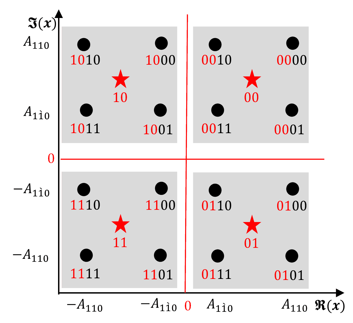
Figure 1: The constellation diagram of the transmitted symbol $x$ for $N=2$.

III-A BER of the first user $\left(U_{1}|_{N=2}\right)$

For the first user, the detection is performed using (3), and thus, no SIC is required. Based on the specific value of $s_{2}$, the IUI caused by $U_{2}$, the symbol $x$ may become one of the four constellation points in the neighborhood of $s_{1}$. The shaded blocks in Fig. 1 show the four possible values that a particular symbol $s_{1}$ may take. For example, given that $s_{1}=10$ then $x|_{s_{1}}\in\left\{1000\text{, }1001\text{, }1010\text{, }1011\right\}$. The amplitudes of the inphase $x_{I}\triangleq\Re\left(x\right)$ and quadrature $x_{Q}\triangleq\Im\left(x\right)$ for each constellation point are defined as

$$A_{u_{1}u_{2}u_{3}}=u_{1}\sqrt{\beta_{1}}+u_{2}\sqrt{\beta_{2}}+u_{3}\sqrt{\beta_{3}}\text{, }u_{i}\in\left\{0,1,\acute{1},2\right\}$$ (5)

where $\acute{1}\triangleq-1$. For example, given that $s_{1}^{(2)}=s_{2}^{(2)}$, then $x=1010$ and $x_{I}=-\sqrt{\beta_{1}}-\sqrt{\beta_{2}}\triangleq A_{\acute{1}\acute{1}0}$, and $x_{Q}=\sqrt{\beta_{1}}+\sqrt{\beta_{2}}\triangleq A_{110}$. It is worth noting that for $N=2$, $u_{3}=0$ regardless the values of $s_{1}$ or $s_{2}$, however, it is used to unify the notation throughout the paper.

The probability of error for each bit actually depends on the values of $s_{1}$ and $s_{2}$. For example, given that $s_{1}^{(2)}$ , the first bit $b_{11}$ might be detected incorrectly if $\hat{s}_{1}=a_{0}$ $(00)$ or $a_{1}$ $(01)$, as shown in Fig. 1. However, $\mathrm{P\!}\left(\hat{s}_{1}=a_{0}\text{ or }a_{1}\right)$, denoted as $\mathrm{P\!}\left(\hat{s}_{1}=a_{0};a_{1}\right),$ depends on $s_{2}$ as well. Therefore, the average BER should consider all possible combinations of $s_{1}$ and $s_{2}$,

$$P_{b_{1i}}=\sum_{l,k}\left(P_{b_{1i}}|_{s_{1}^{(l)}\text{, }s_{2}^{(k)}}\right)\mathrm{P\!}\left(s_{1}^{(l)}\text{, }s_{2}^{(k)}\right).$$ (6)

By noting that $s_{1}$ and $s_{2}$ are independent, then (6) can be written as,

$$P_{b_{1i}}=\frac{1}{16}\sum_{\{l.k\}=0}^{3}\left(P_{b_{1i}}|_{s_{1}^{(l)}\text{, }s_{2}^{(k)}}\right).$$ (7)

$\boldsymbol{Case}$ $\boldsymbol{1}$: $s_{1}^{(2)}$, $s_{2}^{(0)}$: For this case, $x|_{a_{2},a_{0}}=-A_{1\acute{1}0}+jA_{110}$, to simplify th notations $x|_{a_{l},a_{k}}$ is written as $x_{l,k}$. Consequently, the error probability of $b_{11}$ is given by,

$$P_{b_{11}}|_{s_{1}^{(2)}\text{, }s_{2}^{(0)}}=\mathrm{P\!}\left(\hat{s}_{1}=a_{0};a_{1}\right).$$

As can be noted from Fig. 1, $\mathrm{P\!}\left(\hat{s}_{1}=a_{0};a_{1}\right)$ depends only on the inphase component of $\check{r}_{1}$, i.e., $\Re\left(\check{r}_{1}\right)\triangleq\mathfrak{r}_{1}$ and the specific value of $x$. Thus,

$$P_{b_{11}}|_{s_{1}^{(2)}\text{, }s_{2}^{(0)}} =\mathrm{P\!}\left(\mathfrak{r}_{1}\geq 0\right)$$

$$=\mathrm{P\!}\left(-\alpha_{1}A_{1\acute{1}0}+\mathfrak{n}_{1}\geq 0\right)$$

$$=\mathrm{P\!}\left(\mathfrak{n}_{1}\geq\alpha_{1}A_{1\acute{1}0}\right)$$ (8)

where $\mathfrak{r}_{1}=-\alpha_{1}A_{1\acute{1}0}+\mathfrak{n}_{1}$, $\Re\left(\check{w}_{1}\right)\triangleq\mathfrak{n}_{1}$. Therefore,

$$P_{b_{11}}|_{s_{1}^{(2)}\text{, }s_{2}^{(0)}} =\frac{1}{\sqrt{2\pi\sigma_{\mathfrak{n}_{1}}^{2}}}\int_{\alpha_{1}A_{1\acute{1}0}}^{\infty}e^{-\frac{z^{2}}{2\sigma_{\mathfrak{n}_{1}}^{2}}}d\mathfrak{n}_{1}$$

$$=Q\left(\sqrt{\gamma_{1,1}}\right)$$ (9)

where $\gamma_{1,1}=\alpha_{1}^{2}A_{1\acute{1}0}^{2}/\sigma_{\mathfrak{n}_{1}}^{2}$ and $Q\left(.\right)$ denotes the Gaussian $Q$ function.

$\boldsymbol{Case}$ $\boldsymbol{2}$: $s_{1}^{(2)}$, $s_{2}^{(1)}$:

This case is similar to the case of $s_{2}^{(0)}$, hence, the error probability is given by (9) as well.

$\boldsymbol{Case}$ $\boldsymbol{3}$: $s_{1}^{(2)}$, $s_{2}^{(2)}$:

In this case, $x_{2,2}=-A_{110}+jA_{110}$, then the error probability can be expressed as

$$P_{b_{11}}|_{s_{1}^{(2)}\text{, }s_{2}^{(2)}} =\mathrm{P\!}\left(\mathfrak{r}_{1}\geq 0\right)$$

$$=\mathrm{P\!}\left(\mathfrak{n}_{1}\geq\alpha_{1}A_{110}\right).$$ (10)

Following the same approach used to derive (9) gives,

$$P_{b_{11}}|_{s_{1}^{(2)}\text{, }s_{2}^{(2)}}=Q\left(\sqrt{\gamma_{1,2}}\right)$$ (11)

where $\gamma_{1,2}=\alpha_{n}^{2}A_{110}^{2}/\sigma_{\mathfrak{n}_{1}}^{2}$.

$\boldsymbol{Case}$ $\boldsymbol{4}$: $s_{1}^{(2)}$, $s_{2}^{(3)}$:

The probability of error in this case is similar to the case of $s_{1}^{(2)}$, $s_{2}^{(2)}$.

The remaining cases, $\boldsymbol{Case}$ $\boldsymbol{5}$ to $\boldsymbol{Case}$ $\boldsymbol{16}$ are similar to $\boldsymbol{Case}$ $\boldsymbol{1}$ to $\boldsymbol{Case}$ $\boldsymbol{4}$ except that the value of $s_{1}$ is replaced by $a_{0}$, $a_{1}$, $a_{2}$ and $a_{3}$. Substituting the results of the $16$ cases in (7) gives $P_{11}=\frac{1}{2}\left[Q\left(\sqrt{\gamma_{1,1}}\right)+Q\left(\sqrt{\gamma_{1,2}}\right)\right]$. It is also straightforward to show that $P_{12}=P_{11}$. Therefore, the conditional BER of the first user is given:

$$P_{U_{1}} =\frac{1}{2}\left[P_{b_{11}}+Pb_{{}_{12}}\right]$$

$$=\frac{1}{2}\left[Q\left(\sqrt{\gamma_{1,1}}\right)+Q\left(\sqrt{\gamma_{1,2}}\right)\right].$$ (12)

III-B BER of Second User $\left(U_{2}|_{N=2}\right)$

To detect its own symbol $s_{2}$, the second user should initially detect $s_{1}$ as described in (3), and then compute,

$$\hat{s}_{2} =\arg\min_{\tilde{s}_{2}\in\mathbb{S}}\left|r_{2,sic}-\sqrt{\beta_{2}}h_{2}\tilde{s}_{2}\right|^{2}$$

$$=\arg\min_{\tilde{s}_{2}\in\mathbb{S}}\left|x_{sic}h_{2}+w_{2}-\sqrt{\beta_{2}}h_{2}\tilde{s}_{2}\right|^{2}$$ (13)

where $r_{2,sic}=r_{2}-h_{2}\sqrt{\beta_{1}}\hat{s}_{1}$ and $x_{sic}=x-\sqrt{\beta_{1}}\hat{s}_{1}$. Therefore, given that $\hat{s}_{1}=s_{1}$, then $x_{sic}=\sqrt{\beta_{2}}s_{2}$ and $r_{2,sic}$ corresponds to IUI-free QPSK signal. The constellation diagram of $x_{sic}|_{\hat{s}_{1}=s_{1}}$ is shown in Fig. 2. On the other hand, if $\hat{s}_{1}\neq s_{1}$, then $x_{sic}=\sqrt{\beta_{1}}s_{1}+\sqrt{\beta_{2}}s_{2}-\sqrt{\beta_{1}}\hat{s}_{1}$ and its constellation diagram depends on $\hat{s}_{1}$. For example, given that $s_{1}^{(0)}$, $\hat{s}_{1}^{(2)}$, the constellation diagram of $x_{sic}$ becomes as shown in Fig. 2.

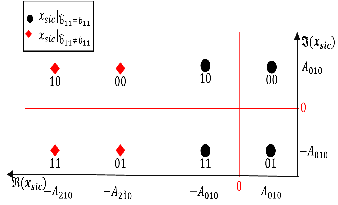
Figure 2: Equivelant constellation of $x_{sic}|_{\hat{s}_{1}=s_{1}}$ and $x_{sic}|_{\hat{s}_{1}\neq s_{1}}$ of the second user, $N=2$.

The BER of $U_{2}$ depends on $s_{1}$, $s_{2}$ and $\hat{s}_{1}$. Therefore, the probability of error should be averaged over all possible combinations,

$$P_{b_{2i}}=\sum_{v,k,l}P_{b_{2i}}|_{s_{1}^{(v)},s_{2}^{(k)},\hat{s}_{1}^{(l)}}\mathrm{P\!}\left(s_{1}^{(v)},s_{2}^{(k)},\hat{s}_{1}^{(l)}\right).$$ (14)

Using the chain rule $\mathrm{P\!}\left(s_{1}^{(v)},s_{2}^{(k)},\hat{s}_{1}^{(l)}\right)=\mathrm{P\!}\left(\hat{s}_{1}^{(a_{l})}|_{s_{1}^{(v)},s_{2}^{(k)}}\right)\mathrm{P\!}\left(s_{1}^{(v)},s_{2}^{(k)}\right)$ and noting that $s_{1}$ and $s_{2}$ are independent, then (14) can be written as,

$$P_{b_{2i}}=\frac{1}{16}\sum_{\left\{k,l,v\right\}=0}^{3}P_{b_{2i}}|_{s_{1}^{(v)},s_{2}^{(k)},\hat{s}_{1}^{(l)}}\mathrm{P\!}\left(\hat{s}_{1}^{(a_{l})}|_{s_{1}^{(v)},s_{2}^{(k)}}\right).$$ (15)

It should be noted that the probability of correct or incorrect detection of $b_{12}$ does not affect the error probability of the second user bits $P_{2i}$. Therefore, it is assumed that $P_{b_{12}}=1$ for all cases.

The case where $v=l$ corresponds to the event that $\hat{s}_{1}=s_{1}$, and the corresponding probabilities can be computed as follows:

$\boldsymbol{Case}$ $\boldsymbol{1}$: $s_{1}^{(0)}\left(b_{11}^{(0)}\right)$, $\hat{s}_{1}^{(0)}\left(\hat{b}_{11}^{(0)}\right)$, $s_{2}^{(2)}$:

The probability $\mathrm{P\!}\left(\hat{b}_{11}^{(0)}=0|_{b_{11}^{(0)}\text{,}s_{2}^{(2)}}\right)$ can be obtained by considering the error probability of $U_{1}$ given that $b_{11}^{(0)}=\hat{b}_{11}^{(0)}$ $\left(s_{1}^{(0)}\right)$ and $s_{2}^{(2)}$. In this case, the conditional error probability of $b_{21}$ can be computed by noting that $P_{b_{21}}|\mathbb{A}_{221}=\mathrm{P\!}\left(\hat{s}_{2}=a_{0};a_{1}|_{\mathbb{A}_{221}}\right)$ where $\mathbb{A}_{221}\rightarrow\left\{b_{11}^{(0)},\hat{b}_{11}^{(0)},s_{2}^{(2)}\right\}$. The transmitted signal amplitude for this case is $x=A_{1\acute{1}0}+jA_{110}$, thus, $x_{sic}=A_{0\acute{1}0}+jA_{010}$ and $r_{2,sic}=\alpha_{2}x_{sic}+w_{2}.$ As can be noted from Fig. 2, $\mathrm{P\!}\left(\hat{s}_{2}=a_{0};a_{1}|_{\mathbb{A}_{221}}\right)$ depends only on the inphase component of $\check{r}_{2,sic}$, i.e., $\Re\left(\check{r}_{2,sic}\right)\triangleq\mathfrak{r}_{2,sic}$. Thus

$$P_{b_{21}}|_{\mathbb{A}_{221}} =\mathrm{P\!}\left(\mathfrak{n}_{2}+\alpha_{2}A_{0\acute{1}0}\geq 0\left|\mathfrak{n}_{2}+\alpha_{2}A_{1\acute{1}0}\geq 0\right.\right)$$

$$=\mathrm{P\!}\left(\mathfrak{n}_{2}\geq\alpha_{2}A_{010}\left|\mathfrak{n}_{2}\geq\alpha_{2}A_{\acute{1}10}\right.\right)$$ (16)

where $\mathfrak{r}_{2,sic}=\alpha_{2}A_{0\acute{1}0}+\mathfrak{n}_{2}$, $\Re\left(\check{w}_{2}\right)\triangleq$ $\mathfrak{n}_{2}$and $-A_{0\acute{1}0}=A_{010}$. Using Bayes’ theorem and considering the results in (15) and (16), we obtain

$$P_{b_{21}}|\mathbb{A}_{221}\mathrm{P\!}\left(\hat{b}_{11}^{\left(0\right)}|_{b_{11}^{(0)},s_{2}^{(2)}}\right) =\mathrm{P\!}\left(\mathfrak{n}_{2}\geq\alpha_{2}A_{\acute{1}10}\right)$$

$$\times\mathrm{P\!}\left(\mathfrak{n}_{2}\geq\alpha_{2}A_{010}\left|\mathfrak{n}_{2}\geq\alpha_{2}A_{\acute{1}10}\right.\right)$$ (17)

By noting that the right hand side of (RHS) of (17) is equal to $\mathrm{P\!}\left(\mathfrak{n}_{2}\geq\alpha_{2}A_{010}\text{, }\mathfrak{n}_{2}\geq\alpha_{2}A_{\acute{1}10}\right)$, then

$$P_{b_{21}}|\mathbb{A}_{221}\mathrm{P\!}\left(\hat{b}_{11}^{(0)}|_{b_{11}^{(0)}\text{,}s_{2}^{(2)}}\right) =\mathrm{P\!}\left(\mathfrak{n}_{2}\geq\alpha_{2}A_{010}\right)$$

$$=Q\left(\sqrt{\gamma_{2,1}}\right)$$ (18)

where $\gamma_{2,1}=\alpha_{2}^{2}A_{010}^{2}/\sigma_{\mathfrak{n}_{2}}^{2}$.

For $b_{22}$, the error probability is obtained using the approach used with $b_{21}$

$$P_{b_{22}}|\mathbb{A}_{221}\mathrm{P\!}\left(\hat{b}_{11}^{(0)}|_{b_{11}^{(0)}\text{,}s_{2}^{(2)}}\right)=\mathrm{P\!}\left(\mathfrak{n}_{2}\geq\alpha_{2}A_{\acute{1}10}\right)\\ \times\mathrm{P\!}\left(\mathfrak{q}_{2}+\alpha_{2}A_{010}\leq 0\left|\mathfrak{n}_{2}\geq\alpha_{2}A_{\acute{1}10}\right.\right).$$ (19)

As the RHS of (19) can be simplified to $\mathrm{P\!}\left(\mathfrak{q}_{2}\leq\alpha_{2}A_{0\acute{1}0},\mathfrak{n}_{2}\geq\alpha_{2}A_{\acute{1}10}\right)$, then

$$P_{b_{22}}|\mathbb{A}_{221}\mathrm{P\!}\left(\hat{b}_{11}^{(0)}|_{b_{11}^{(0)},s_{2}^{(2)}}\right)=Q\left(\sqrt{\gamma_{2,1}}\right)\left(1-Q\left(\sqrt{\gamma_{2,2}}\right)\right)$$ (20)

where $\mathfrak{q}_{2}\triangleq\mathfrak{I}\left(\check{w}_{2}\right)$ and $\gamma_{2,2}=\alpha_{2}^{2}A_{1\acute{1}0}^{2}/\sigma_{\mathfrak{n}_{2}}^{2}.$

$\boldsymbol{Case}$ $\boldsymbol{2}$: $s_{1}^{(0)}\left(b_{11}^{(0)}\right)$, $\hat{s}_{1}^{(0)}$ $\left(\hat{b}_{11}^{(0)}\right)$, $s_{2}^{(0)}$:

In this case, $\left(P_{21}|_{\mathbb{A}_{222}}\right)\mathrm{P\!}\left(\hat{b}_{11}^{(0)}|_{b_{11}^{(0)},s_{2}^{(0)}}\right)$ where $\mathbb{A}_{222}\rightarrow\left\{b_{11}^{(0)},\hat{b}_{11}^{(0)},s_{2}^{(0)}\right\}$ is computed for $x_{sic}=A_{110}+jA_{110}$ and $r_{2,sic}=\alpha_{2}x_{sic}+w_{2}$,

$$P_{b_{21}}|_{\mathbb{A}_{222}}\mathrm{P\!}\left(\hat{b}_{11}^{(0)}|_{b_{11}^{(0)}\text{,}s_{2}^{(0)}}\right)=\mathrm{P\!}\left(\mathfrak{n}_{2}+\alpha_{2}A_{110}\geq 0\right)\\ \times\mathrm{P\!}\left(\mathfrak{n}_{2}+\alpha_{2}A_{010}\leq 0\left|\mathfrak{n}_{2}+\alpha_{2}A_{110}\geq 0\right.\right)$$ (21)

Since the RHS of (21) can be simplified to $\mathrm{P\!}\left(\mathfrak{n}_{2}\leq\alpha_{2}A_{0\acute{1}0},\mathfrak{n}_{2}\geq\alpha_{2}A_{\acute{1}\acute{1}0}\right)$, then

$$P_{b_{21}}|_{\mathbb{A}_{222}}\mathrm{P\!}\left(\hat{b}_{11}^{(0)}|_{b_{11}^{(0)}\text{,}s_{2}^{(0)}}\right)=Q\left(\sqrt{\gamma_{2,1}}\right)-Q\left(\sqrt{\gamma_{2,3}}\right)$$ (22)

where $\gamma_{2,3}=\alpha_{2}^{2}A_{110}^{2}/\sigma_{\mathfrak{n}_{2}}^{2}$.

For $b_{22}$, the error probability is given by

$$P_{b_{22}}|_{\mathbb{A}_{222}}\mathrm{P\!}\left(\hat{b}_{11}^{(0)}|_{b_{11}^{(0)}\text{,}s_{2}^{(0)}}\right)=\mathrm{P\!}\left(\mathfrak{n}_{2}+\alpha_{2}A_{110}\geq 0\right)\\ \times\mathrm{P\!}\left(\mathfrak{q}_{2}+\alpha_{2}A_{010}\leq 0\left|\mathfrak{n}_{2}+\alpha_{2}A_{110}\geq 0\right.\right).$$ (23)

The RHS of (23) can be simplified to $\mathrm{P\!}\left(\mathfrak{q}_{2}\leq\alpha_{2}A_{0\acute{1}0}\right)\mathrm{P\!}\left(\mathfrak{n}_{2}\geq\alpha_{2}A_{\acute{1}\acute{1}0}\right)$, and thus

$$P_{b_{22}}|_{\mathbb{A}_{222}}\mathrm{P\!}\left(\hat{b}_{11}^{(0)}|_{b_{11}^{(0)},s_{2}^{(0)}}\right)=Q\left(\sqrt{\gamma_{2,1}}\right)\left(1-Q\left(\sqrt{\gamma_{2,3}}\right)\right).$$ (24)

The remaining cases, $\boldsymbol{Case}$ $\boldsymbol{3}$ to $\boldsymbol{Case}$ $\boldsymbol{9}$ where the constellation points are $0110$, $0011$, $0111$, $1000$, $1001$, $1100$, $1101$ are similar to $\boldsymbol{Case}$ $\boldsymbol{1,}$ and $\boldsymbol{Case}$ $\boldsymbol{10}$ to $\boldsymbol{Case}$ $\boldsymbol{16}$ where the constellation points are $0001$, $0100$, $0101$, $1010$, $1011$, $1110$, $1111$ are similar to $\boldsymbol{Case}$ $\boldsymbol{2}$. By using (15), the BER of the second user given that $\hat{b}_{11}=b_{11}$ can be expressed as

$$P_{U_{2}}^{\left(1\right)}=\frac{1}{2}Q\left(\sqrt{\gamma_{2,1}}\right)\left[2-Q\left(\sqrt{\gamma_{2,2}}\right)-Q\left(\sqrt{\gamma_{2,3}}\right)\right]\\ -\frac{1}{2}Q\left(\sqrt{\gamma_{2,3}}\right).$$ (25)

The constellation diagram of $x_{sic}$, after subtracting $\hat{s}_{1}|_{\hat{b}_{11}\neq b_{11}}$ is shown in Fig. 2 (solid diamonds). The total error probability of the second user when $\hat{b}_{11}\neq b_{11}$ can be derived by considering all the cases in (15).

$\boldsymbol{Case}$ $\boldsymbol{1}$: $s_{1}^{(0)}$ $\left(b_{11}^{(0)}\right)$, $\hat{s}_{1}^{(2)}$ $\left(\hat{b}_{11}^{(1)}\right)$, $s_{2}^{(2)}$:

The transmitted signal amplitude of this point is $x=A_{1\acute{1}0}+jA_{110}$, thus, $x_{I,sic}=A_{2\acute{1}0}$. The error probability for this case is

$$P_{b_{21}}|_{\mathbb{B}_{221}}\mathrm{P\!}\left(\hat{b}_{11}^{(1)}|_{b_{11}^{(0)}\text{, }s_{2}^{(2)}}\right)=\mathrm{P\!}\left(\mathfrak{n}_{2}+\alpha_{2}A_{1\acute{1}0}\leq 0\right)\\ \times\mathrm{P\!}\left(\mathfrak{n}_{2}+\alpha_{2}A_{2\acute{1}0}\geq 0\left|\mathfrak{n}_{2}+\alpha_{2}A_{1\acute{1}0}\leq 0\right.\right)$$ (26)

where $\mathbb{B}_{221}\rightarrow\left\{b_{11}^{(0)},\hat{b}_{11}^{(1)},s_{2}^{(2)}\right\}$. The RHS of (26) can be simplified to $\mathrm{P\!}\left(\alpha_{2}A_{\acute{2}10}\leq\mathfrak{n}_{2}\leq\alpha_{2}A_{\acute{1}10}\right)$. Thus,

$$P_{b_{21}}|_{\mathbb{B}_{221}}\mathrm{P\!}\left(\hat{b}_{11}^{(1)}|_{b_{11}^{(0)}\text{, }s_{2}^{(2)}}\right)=Q\left(\sqrt{\gamma_{2,2}}\right)-Q\left(\sqrt{\gamma_{2,4}}\right)$$ (27)

where $\gamma_{2,4}=\alpha_{2}^{2}A_{2\acute{1}0}^{2}/\sigma_{\mathfrak{n}_{2}}^{2}$.

The error probability of $b_{22}$ is obtained as

$$P_{b_{22}}|_{\mathbb{B}_{221}}\mathrm{P\!}\left(\hat{b}_{11}^{(1)}|_{b_{11}^{(0)}\text{, }s_{2}^{(2)}}\right)=\mathrm{P\!}\left(\mathfrak{n}_{2}+\alpha_{2}A_{1\acute{1}0}\leq 0\right)\\ \times\mathrm{P\!}\left(\mathfrak{q}_{2}+\alpha_{2}A_{010}\leq 0\left|\mathfrak{n}_{2}+\alpha_{2}A_{1\acute{1}0}\leq 0\right.\right)$$ (28)

By noting that the RHS of (28) can be simplified to $\mathrm{P\!}\left(\mathfrak{q}_{2}\leq\alpha_{2}A_{0\acute{1}0},\mathfrak{n}_{2}\leq\alpha_{2}A_{\acute{1}10}\right)$, then

$$P_{b_{22}}|_{\mathbb{B}_{221}}\mathrm{P\!}\left(\hat{b}_{11}^{(1)}|_{b_{11}^{(0)}\text{, }s_{2}^{(2)}}\right)=Q\left(\sqrt{\gamma_{2,1}}\right)Q\left(\sqrt{\gamma_{2,2}}\right).$$ (29)

$\boldsymbol{Case}$ $\boldsymbol{2}$: $s_{1}^{(0)}$ $\left(b_{11}^{(0)}\right)$, $\hat{s}_{1}^{(2)}$ $\left(\hat{b}_{11}^{(1)}\right)$, $s_{2}^{(0)}$:

The error probability of this case can be computed as

$$P_{b_{21}}|_{\mathbb{B}_{222}}\mathrm{P\!}\left(\hat{b}_{11}^{(1)}|_{b_{11}^{(0)}\text{,}s_{2}^{(0)}}\right)=\mathrm{P\!}\left(\mathfrak{n}_{2}+\alpha_{2}A_{110}\leq 0\right)\\ \times\mathrm{P\!}\left(\mathfrak{n}_{2}+\alpha_{2}A_{210}\leq 0\left|\mathfrak{n}_{2}+\alpha_{2}A_{110}\leq 0\right.\right)$$ (30)

The RHS of (30) can be expressed as $\mathrm{P\!}\left(\mathfrak{n}_{2}\leq\alpha_{2}A_{\acute{2}\acute{1}0},\mathfrak{n}_{2}\leq\alpha_{2}A_{\acute{1}\acute{1}0}\right)$, and hence,

$$P_{b_{21}}|_{\mathbb{B}_{222}}\mathrm{P\!}\left(\hat{b}_{11}^{(1)}|_{b_{11}^{(0)}\text{,}s_{2}^{(0)}}\right)=Q\left(\sqrt{\gamma_{2,5}}\right)$$ (31)

where $\gamma_{2,5}=\alpha_{2}^{2}A_{210}^{2}/\sigma_{\mathfrak{n}_{2}}^{2}$, and $\mathbb{B}_{222}\rightarrow\left\{b_{11}^{(0)},\hat{b}_{11}^{(1)},s_{2}^{(0)}\right\}.$

For $b_{22}$, the error probability is evaluated as

$$P_{b_{22}}|_{\mathbb{B}_{222}}\mathrm{P\!}\left(\hat{b}_{11}^{(1)}|_{b_{11}^{(0)}\text{,}s_{2}^{(0)}}\right)=\mathrm{P\!}\left(\mathfrak{n}_{2}+\alpha_{2}A_{110}\leq 0\right)\\ \times\mathrm{P\!}\left(\mathfrak{q}_{2}+\alpha_{2}A_{010}\leq 0\left|\mathfrak{n}_{2}+\alpha_{2}A_{110}\leq 0\right.\right)$$ (32)

Since the RHS of (32) can be simplified to $\mathrm{P\!}\left(\mathfrak{q}_{2}\leq\alpha_{2}A_{0\acute{1}0},\mathfrak{n}_{2}\leq\alpha_{2}A_{\acute{1}\acute{1}0}\right)$, then

$$P_{b_{22}}|_{\mathbb{B}_{222}}\mathrm{P\!}\left(\hat{b}_{11}^{(1)}|_{b_{11}^{(0)}\text{,}s_{2}^{(0)}}\right)=Q\left(\sqrt{\gamma_{2,1}}\right)Q\left(\sqrt{\gamma_{2,3}}\right).$$ (33)

For the remaining cases, $\boldsymbol{Case}$ $\boldsymbol{3}$ to $\boldsymbol{Case}$ $\boldsymbol{9}$ where the associated symbols are $0011$, $0110$, $0111$, $1000$, $1001$, $1100$, and $1101$ are identical to $\boldsymbol{Case}$ $\boldsymbol{1}$. $\boldsymbol{Case}$ $\boldsymbol{\boldsymbol{1}0}$ to $\boldsymbol{Case}$ $\boldsymbol{\boldsymbol{1}6}$ where the constellation points are $0001$, $0100$, $0101$, $1010$, $1011$, $1110$, and $1111$ are similar to $\boldsymbol{Case}$ $\boldsymbol{2}$. Therefore, the total error probability when $\hat{b}_{11}$ $\neq b_{11}$can be expressed as

$$P_{U_{2}}^{\left(2\right)}=Q\left(\sqrt{\gamma_{2,1}}\right)\left[Q\left(\sqrt{\gamma_{2,2}}\right)+Q\left(\sqrt{\gamma_{2,3}}\right)\right]+Q\left(\sqrt{\gamma_{2,2}}\right)\\ -Q\left(\sqrt{\gamma_{2,4}}\right)+Q\left(\sqrt{\gamma_{2,5}}\right).$$ (34)

Finally, the exact total BER for the second user is given as the sum of the results of the two scenarios where $\hat{b}_{11}=b_{11}$ and $\hat{b}_{11}\neq b_{11}$,

$$P_{U_{2}}=\frac{1}{2}\sum_{i=1}^{5}v_{i}Q\left(\sqrt{\gamma_{2,i}}\right)\text{, }\mathbf{v}=\left[2,1,-1,-1,1\right].$$ (35)

III-C Average BER, $N=2$

The average BER can be evaluated by averaging over the PDFs of all $\gamma_{n,c}$ values, which are given in Appendix I. Therefore, by substituting $N=2$ and $n=\left[1,2\right]$ in the ordered PDF in  (93), the exact average BER of the first and second users can be simplified to

$$\overline{P}_{U_{1}}=\frac{1}{\pi\Gamma(m)}\sum_{c=1}^{2}\sum_{k=0}^{2}\sum_{i=0}^{\infty}\left(-1\right)^{k}S_{i}\left(\frac{m}{\overline{\gamma}_{1,c}}\right)^{m(1+k)}\\ \times\int_{0}^{\frac{\pi}{2}}\frac{\left(i+mk\right)!}{\left(\frac{1}{2\sin^{2}\left(\psi_{1,c}\right)}+\frac{m\text{ }\left(1+k\right)}{\overline{\gamma}_{1,c}}\right)^{i+mk+1}}d\psi_{n,c}$$ (36)

and

$$\bar{P}_{U_{2}}=\frac{1}{\pi\Gamma(m)}\sum\limits_{c=1}^{5}\sum_{i=0}^{\infty}v_{c}S_{i}\left(\frac{m}{\overline{\gamma}_{2,c}}\right)^{2m}\\ \times\int_{0}^{\frac{\pi}{2}}\frac{\left(i+m\right)!}{\left(\frac{1}{2\sin^{2}\left(\psi_{2,c}\right)}+\frac{2m\text{ }}{\overline{\gamma}_{2,c}}\right)^{i+m+1}}d\psi_{2,c}$$ (37)

where $\mathbf{v}=\left[2,1,-1,-1,1\right]$. It is interesting to note that for the special case of Rayleigh fading channel where $m=1$, the BER for both users can be expressed in closed-form as,

$$\bar{P}_{U_{1}}=\frac{1}{4}\sum_{c=1}^{2}\left(1-\frac{1}{\sqrt{\frac{1}{\overline{\gamma}_{1,c}}+1}}\right)$$ (38)

and

$$\bar{P}_{U_{2}}=\frac{1}{2}\sum_{c=1}^{5}v_{c}\left(\sqrt{\frac{\overline{\gamma}_{2,c}}{\overline{\gamma}_{2,c}+1}}-\sqrt{\frac{8\overline{\gamma}_{2,c}}{2\overline{\gamma}_{2,c}+1}}+1\right)$$ (39)

where $\mathbf{v}=\left[2,1,-1,-1,1\right]$.

IV NOMA Bit Error Rate (BER) Analysis: Three Users ($N=3)$

This section presents the derivation of the BER for a three-users NOMA system, $N=3$, which generally follows the derived $N=2$ case. The transmitted signal constellation is given in Fig. 3. The first, second, and third users’ signals are shown in the form of $\left[s_{1},s_{2},s_{3}\right]$. The binary bit representation for the three users are represented as $\begin{bmatrix}b_{11}&b_{12}&b_{21}&b_{22}&b_{31}&b_{32}\end{bmatrix}$, for each bit $b_{ni}$, $n=\left[1\text{, }2,3\right]$, and $i=\left[1,2\right]$ which denotes bits’ indices.

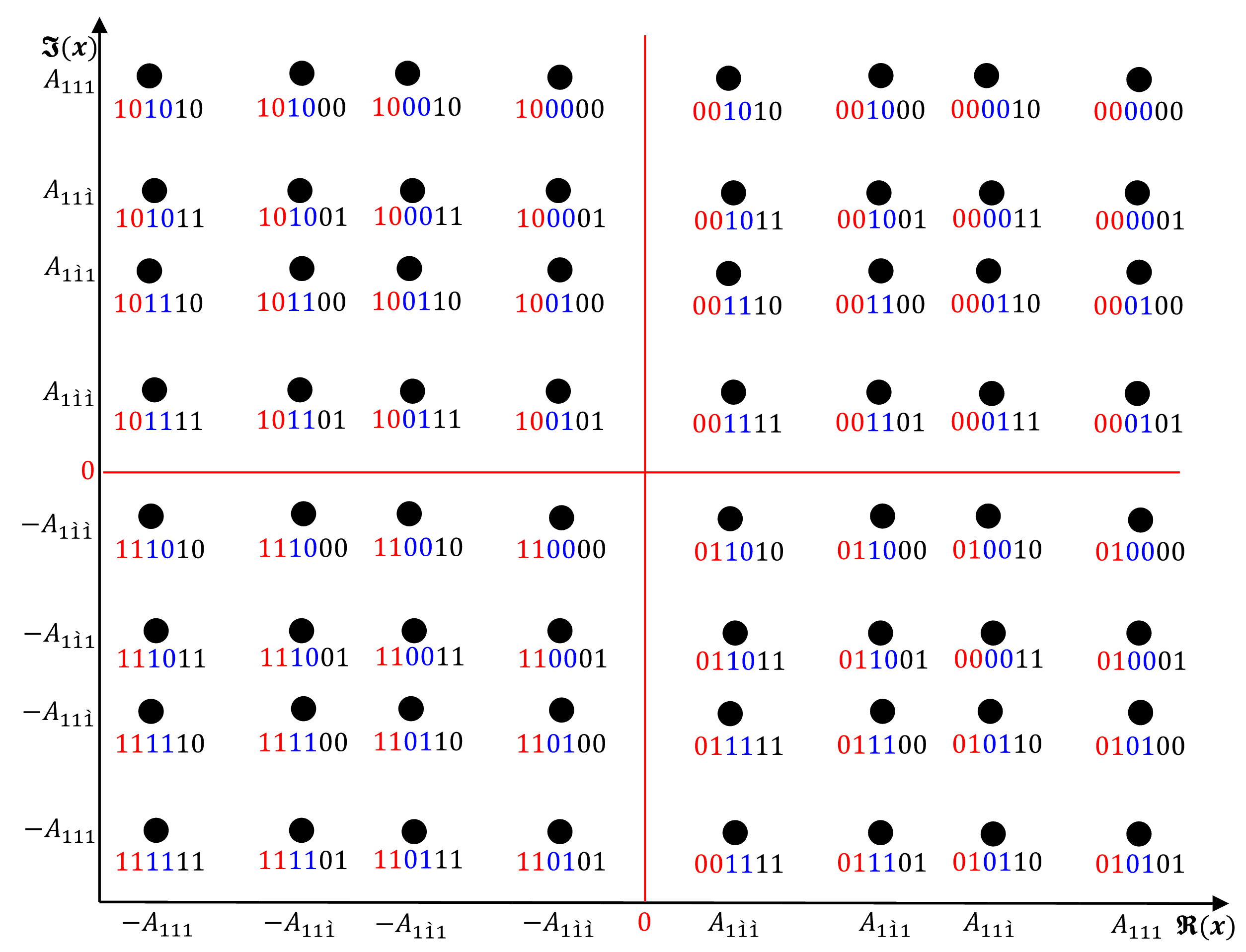
Figure 3: The transmitted superimposed signal constellation for $N=3$.

IV-A BER of First User $\left(U_{1}|_{N=3}\right)$

The error probability of the first user can be obtained directly from Fig. 3. The probability of error for each bit depends on the values of $s_{1}$, $s_{2}$ and $s_{3}$. For example, given that $s_{1}^{\left(2\right)}$, $s_{3}^{(3)}$, the first bit $b_{11}$ might be detected incorrectly if $\hat{s}_{1}=a_{0}$ $(00)$ or $a_{1}$ $(01)$, as shown in Fig. 3. Therefore, the average BER should consider all possible combinations of $s_{1}$, $s_{2}$ and $s_{3}$,

$$P_{b_{1i}}=\sum_{c,k,v}P_{b_{1i}}|_{s_{1}^{(c)},s_{2}^{(k)},s_{3}^{(v)}}\mathrm{P\!}\left(s_{1}^{(c)},s_{2}^{(k)},s_{3}^{(v)}\right).$$ (40)

Because $s_{1}$, $s_{2}$ and $s_{3}$ are mutually independent, (40) can be written as

$$P_{b_{1i}}=\frac{1}{64}\sum_{\left\{c,k,v\right\}=0}^{3}P_{b_{1i}}|_{s_{1}^{(c)},s_{2}^{(k)},s_{3}^{(v)}}.$$ (41)

The error probability of the first user is derived by considering all possible combinations, which can be derived as follows:

$\boldsymbol{Case}$ $\boldsymbol{1}$: $s_{1}^{(0)}$, $s_{2}^{(2)}$, $s_{3}^{(2)}$:

For this case, $x=A_{1\acute{1}\acute{1}}+jA_{111}$, consequently, the error probability of $b_{11}$ is given by,

$$P_{b_{1i}}|_{s_{1}^{(0)},s_{2}^{(2)},s_{3}^{(2)}}=\mathrm{P\!}\left(\hat{s}_{1}=a_{2};a_{3}\right)$$ (42)

As can be noted from Fig. 3, $\mathrm{P\!}\left(\hat{s}_{1}=a_{2};a_{3}\right)$ depends only on the inphase component of $\check{r}_{1}$, i.e., $\mathfrak{r}_{1}=\alpha_{1}A_{1\acute{1}\acute{1}}+\mathfrak{n}_{1}$, and the specific value of $x$. Thus,

$$P_{b_{1i}}|_{s_{1}^{(0)},s_{2}^{(2)},s_{3}^{(2)}} =\mathrm{P\!}\left(\mathfrak{r}_{1}\leq 0\right)$$

$$=\mathrm{P\!}\left(\alpha_{1}A_{1\acute{1}\acute{1}}+\mathfrak{n}_{1}\leq 0\right)$$

$$=Q\left(\sqrt{\gamma_{3,1}}\right).$$ (43)

Following the same approach, Table I shows the summary of $\boldsymbol{Case}$ $\mathbf{2}$ to $\boldsymbol{Case}$ $\mathbf{4}$. The remaining $60$ cases, $\boldsymbol{Case}$ $\boldsymbol{5}$ to $\boldsymbol{64}$ in Fig. 3, can be obtained following the same approach, and hence, the total BER of the first user can be expressed as

$$P_{U_{1}}=\frac{1}{4}\sum\limits_{v=1}^{4}Q\left(\sqrt{\gamma_{3,v}}\right).$$ (44)

TABLE I: Summary of cases 1 to 4 for $U_{1}$, $N=3.$

$Case$ $(v)$	$x$	$s_{1},s_{2},s_{3}$	$\gamma_{3,v}$
$1$	$A_{1\acute{1}\acute{1}}+jA_{111}$	$a_{0},a_{2},a_{2}$	$\frac{\alpha_{1}^{2}A_{1\acute{1}\acute{1}}^{2}}{\sigma_{\mathfrak{n}_{1}}^{2}}$
$2$	$A_{1\acute{1}1}+jA_{111}$	$a_{0},a_{2},a_{0}$	$\frac{\alpha_{1}^{2}A_{1\acute{1}1}^{2}}{\sigma_{\mathfrak{n}_{1}}^{2}}$
$3$	$A_{11\acute{1}}+jA_{111}$	$a_{0},a_{0},a_{2}$	$\frac{\alpha_{1}^{2}A_{11\acute{1}}^{2}}{\sigma_{\mathfrak{n}_{1}}^{2}}$
$4$	$A_{111}+jA_{111}$	$a_{0},a_{0},a_{0}$	$\frac{\alpha_{1}^{2}A_{111}^{2}}{\sigma_{\mathfrak{n}_{1}}^{2}}$

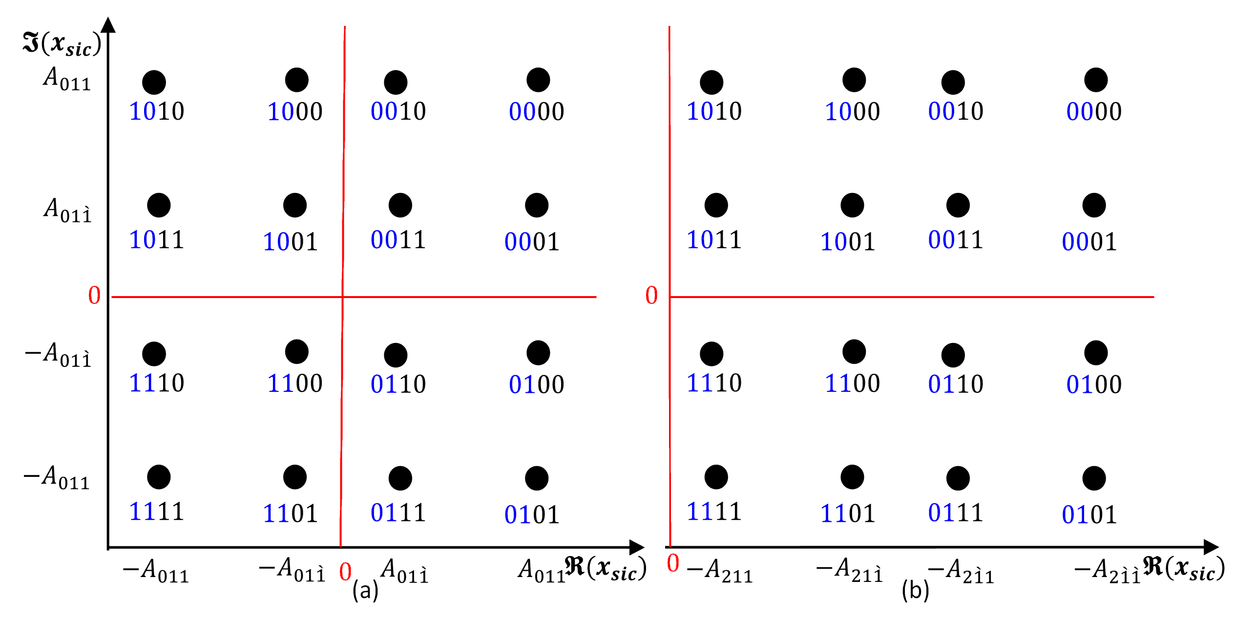
Figure 4: Equivelant constellation of (a) $x_{sic}|_{\hat{b}_{11}=b_{11}}$ and (b) $x_{sic}|_{\hat{b}_{11}\neq b_{11}}$ of the second user, $N=3$.

IV-B BER of Second User $\left(U_{2}|_{N=3}\right)$

The BER of the second user depends on the detection result of the first user and the SIC process as illustrated in Fig. 4. The first case is when $\hat{s}_{1}=s_{1}$, which is represented in Fig. 4.a while the other case is when $\hat{s}_{1}\neq s_{1}$, which is depicted in Fig. 4.b. To detect its own symbol $s_{2}$, the second user should follow the SIC process described in (13). It should be noted that the error probability of the second user is not affected by the detection result of the second bit of the first user $b_{12}$.

The BER of $U_{2}$ depends on $s_{1}$, $\hat{s}_{1}$, $s_{2}$ and $s_{3}$. Therefore, the average BER for $b_{2i}$ is the average of all possible combinations,

$$P_{b_{2i}} =\sum_{g,l,k,v}P_{b_{2i}}|_{s_{1}^{(g)},s_{2}^{(k)},s_{3}^{(v)},\hat{s}_{1}^{(l)}}\mathrm{P\!}\left(s_{1}^{(g)},s_{2}^{(k)},s_{3}^{(v)},\hat{s}_{1}^{(l)}\right)$$

$$=\sum_{g,l,k,v}P_{b_{2i}}|_{s_{1}^{(g)},s_{2}^{(k)},s_{3}^{(v)},\hat{s}_{1}^{(l)}}\mathrm{P\!}\left(\hat{s}_{1}^{(l)}|_{s_{1}^{(g)},s_{2}^{(k)},s_{3}^{(v)}}\right)$$

$$\text{ \ \ \ \ \ \ \ \ \ \ \ \ \ \ \ \ \ \ \ \ \ \ \ \ \ \ \ \ \ \ \ \ \ }\times\mathrm{P\!}\left(s_{1}^{(g)},s_{2}^{(k)},s_{3}^{(v)}\right)$$

$$=\frac{1}{64}\sum_{\left\{g,l,k,v\right\}=0}^{3}P_{b_{2i}}|_{s_{1}^{(g)},s_{2}^{(k)},s_{3}^{(v)},\hat{s}_{1}^{(l)}}$$

$$\text{ \ \ \ \ \ \ \ \ \ \ \ \ \ \ \ \ \ \ \ \ \ \ \ \ \ \ \ \ \ \ \ \ }\times\mathrm{P\!}\left(\hat{s}_{1}^{(l)}|_{s_{1}^{(g)},s_{2}^{(k)},s_{3}^{(v)}}\right)$$ (45)

With the aid of Fig. 4.a, the total BER for the scenario where $\hat{s}_{1}=s_{1}$, or more specifically, where $\hat{b}_{11}=b_{11}$ is obtained as follows:

$\boldsymbol{Case}$ $\boldsymbol{1}$: $s_{1}^{(0)}$ $\left(b_{11}^{(0)}\right)$, $\hat{s}_{1}^{(0)}$ $\left(\hat{b}_{11}^{(0)}\right)$, $s_{2}^{(2)}$, $s_{3}^{(2)}$:

The probability $P_{b_{21}}|_{\mathbb{A}_{321}}$, $\mathbb{A}_{321}\rightarrow\left\{b_{11}^{(0)},\hat{b}_{11}^{(0)},s_{2}^{(2)},s_{3}^{(2)}\right\}$ can be evaluated by considering the error probability of $U_{1}$ given $\mathbb{A}_{321}$. In this case $P_{b_{21}}$ can be computed by noting that $P_{b_{21}}|_{\mathbb{A}_{321}}=\mathrm{P\!}\left(\hat{s}_{2}=a_{0};a_{1}|_{b_{11}^{(0)}\text{, }\hat{b}_{11}^{(0)}\text{, }s_{2}^{(2)}\text{, }s_{3}^{(2)}}\right)$. The transmitted signal amplitude of this case is $x=A_{1\acute{1}\acute{1}}+jA_{111}$, thus, $x_{sic}=A_{0\acute{1}\acute{1}}+jA_{011}$ and $r_{2,sic}=\alpha_{2}x_{sic}+w_{2}$. Therefore,

$$P_{b_{21}}|_{\mathbb{A}_{321}} =\mathrm{P\!}\left(\mathfrak{n}_{2}+\alpha_{2}A_{0\acute{1}\acute{1}}\geq 0\left|\mathfrak{n}_{2}+A_{1\acute{1}\acute{1}}\geq 0\right.\right)$$

$$=\mathrm{P\!}\left(\mathfrak{n}_{2}\geq\alpha_{2}A_{011}\left|\mathfrak{n}_{2}\geq\alpha_{2}A_{\acute{1}11}\right.\right)$$ (46)

where $\mathfrak{r}_{2,sic}=\alpha_{2}A_{0\acute{1}\acute{1}}+\mathfrak{n}_{2}$. Therefore,

$$P_{b_{21}}|_{\mathbb{A}_{321}}\mathrm{P\!}\left(\hat{b}_{11}^{(0)}|_{b_{11}^{(0)}\text{,}s_{2}^{(2)},s_{3}^{(2)}}\right) =\mathrm{P\!}\left(\mathfrak{n}_{2}\geq\alpha_{2}A_{011}\right)$$

$$=Q\left(\sqrt{\gamma_{3,5}}\right)$$ (47)

where $\gamma_{3,5}=\alpha_{2}^{2}A_{011}^{2}/\sigma_{\mathfrak{n}_{2}}^{2}$.

For $b_{22\text{ }}$bit, the error probability is obtained in a similar approach as $b_{21}$

$$P_{b_{22}}|_{\mathbb{A}_{321}}\mathrm{P\!}\left(\hat{b}_{11}^{(0)}|_{b_{11}^{(0)}\text{,}s_{2}^{(2)},s_{3}^{(2)}}\right) =\mathrm{P\!}\left(\mathfrak{q}_{2}\leq\alpha_{2}A_{0\acute{1}\acute{1}}\right)\mathrm{P\!}\left(\mathfrak{n}_{2}\geq\alpha_{2}A_{\acute{1}11}\right)$$

$$=Q\left(\sqrt{\gamma_{3,5}}\right)\left(1-Q\left(\sqrt{\gamma_{3,1}}\right)\right).$$ (48)

$\boldsymbol{Case}$ $\boldsymbol{2}$: $s_{1}^{(0)}$ $\left(b_{11}^{(0)}\right)$, $\hat{s}_{1}^{(0)}$ $\left(\hat{b}_{11}^{(0)}\right)$, $s_{2}^{(2)}$, $s_{3}^{(0)}$:

Based on Fig. 4.a, the error probability of $b_{21}$ is given by

$$P_{b_{21}}|_{\mathbb{A}_{321}}\mathrm{P\!}\left(\hat{b}_{11}^{(0)}|_{b_{11}^{(0)}\text{,}s_{2}^{(2)},s_{3}^{(0)}}\right)=\mathrm{P\!}\left(\mathfrak{n}_{2}\geq\alpha_{2}A_{\acute{1}1\acute{1}}\right)\\ \times\mathrm{P\!}\left(\mathfrak{n}_{2}\geq\alpha_{2}A_{01\acute{1}}\left|\mathfrak{n}_{2}\geq\alpha_{2}A_{\acute{1}1\acute{1}}\right.\right)$$ (49)

By noting that the RHS of (49) can be simplified to $\mathrm{P\!}\left(\mathfrak{n}_{2}\geq\alpha_{2}A_{01\acute{1}}\right)$, and consequently it is straightforward to show that

$$P_{b_{21}}|_{\mathbb{A}_{322}}\mathrm{P\!}\left(\hat{b}_{11}^{(0)}|_{b_{11}^{(0)}\text{,}s_{2}^{(2)},s_{3}^{(0)}}\right)=Q\left(\sqrt{\gamma_{3,6}}\right)$$ (50)

where $\gamma_{3,6}=\alpha_{2}^{2}A_{01\acute{1}}^{2}/\sigma_{\mathfrak{n}_{2}}^{2}$, $\mathbb{A}_{322}\rightarrow\left\{b_{11}^{\left(0\right)},\hat{b}_{11}^{(0)},s_{2}^{(2)},s_{3}^{(0)}\right\}$.

For $b_{22\text{ }}$bit, the error probability is obtained as

$$P_{b_{22}}|_{\mathbb{A}_{322}}\mathrm{P\!}\left(\hat{b}_{11}^{(0)}|_{b_{11}^{(0)}\text{,}s_{2}^{(2)},s_{3}^{(0)}}\right) =\mathrm{P\!}\left(\mathfrak{q}_{2}\leq\alpha_{2}A_{0\acute{1}\acute{1}}\right)\mathrm{P\!}\left(\mathfrak{n}_{2}\geq\alpha_{2}A_{\acute{1}1\acute{1}}\right)$$

$$=Q\left(\sqrt{\gamma_{3,5}}\right)\left(1-Q\left(\sqrt{\gamma_{3,2}}\right)\right).$$ (51)

$\boldsymbol{Case}$ $\boldsymbol{3}$: $s_{1}^{(0)}$ $\left(b_{11}^{(0)}\right)$, $\hat{s}_{1}^{(0)}$ $\left(\hat{b}_{11}^{(0)}\right)$, $s_{2}^{(0)}$, $s_{3}^{(2)}$:

The error probability of this case can be evaluated as

$$P_{b_{21}}|_{\mathbb{A}_{323}}\mathrm{P\!}\left(\hat{b}_{11}^{(0)}|_{b_{11}^{(0)},s_{2}^{(0)},s_{3}^{(2)}}\right) =\mathrm{P\!}\left(\alpha_{2}A_{\acute{1}\acute{1}1}\leq\mathfrak{n}_{2}\leq\alpha_{2}A_{0\acute{1}1}\right)$$

$$=Q\left(\sqrt{\gamma_{3,6}}\right)-Q\left(\sqrt{\gamma_{3,3}}\right).$$ (52)

where $\mathbb{A}_{323}\rightarrow\left\{b_{11}^{(0)},\hat{b}_{11}^{(0)},s_{2}^{(0)},s_{3}^{(2)}\right\}.$

For $b_{22\text{ }}$bit, the error probability is obtained as

$$P_{b_{22}}|_{\mathbb{A}_{323}}\mathrm{P\!}\left(\hat{b}_{11}^{(0)}|_{b_{11}^{(0)},s_{2}^{(0)},s_{3}^{(2)}}\right) =\mathrm{P\!}\left(\mathfrak{q}_{2}\leq\alpha_{2}A_{0\acute{1}\acute{1}}\right)$$

$$\text{ \ \ \ \ \ \ \ \ \ \ \ \ }\times\mathrm{P\!}\left(\mathfrak{n}_{2}\geq\alpha_{2}A_{\acute{1}\acute{1}1}\right)$$

$$=Q\left(\sqrt{\gamma_{3,5}}\right)\left(1-Q\left(\sqrt{\gamma_{3,3}}\right)\right).$$ (53)

$\boldsymbol{Case}$ $\boldsymbol{4}$: $s_{1}^{(0)}$ $\left(b_{11}^{(0)}\right)$, $\hat{s}_{1}^{(0)}$ $\left(\hat{b}_{11}^{(0)}\right)$, $s_{2}^{(0)}$, $s_{3}^{(0)}$:

The error probability of $b_{21}$ can be evaluated as

$$P_{b_{21}}|_{\mathbb{A}_{324}}\mathrm{P\!}\left(\hat{b}_{11}^{(0)}|_{b_{11}^{(0)}\text{,}s_{2}^{(0)},s_{3}^{(0)}}\right) =\mathrm{P\!}\left(\alpha_{2}A_{\acute{1}\acute{1}\acute{1}}\leq\mathfrak{n}_{2}\leq\alpha_{2}A_{0\acute{1}\acute{1}}\right)$$

$$=Q\left(\sqrt{\gamma_{3,5}}\right)-Q\left(\sqrt{\gamma_{3,4}}\right).$$ (54)

where $\mathbb{A}_{324}\rightarrow\left\{b_{11}^{(0)},\hat{b}_{11}^{(0)},s_{2}^{(0)},s_{3}^{(0)}\right\}$.

For $b_{22\text{ }}$, the error probability can be expressed as

$$P_{b_{22}}|_{\mathbb{A}_{324}}\mathrm{P\!}\left(\hat{b}_{11}^{(0)}|_{b_{11}^{(0)}\text{,}s_{2}^{(0)},s_{3}^{(0)}}\right) =\mathrm{P\!}\left(\mathfrak{q}_{2}\leq\alpha_{2}A_{0\acute{1}\acute{1}}\right)\mathrm{P\!}\left(\mathfrak{n}_{2}\geq\alpha_{2}A_{\acute{1}\acute{1}\acute{1}}\right)$$

$$=Q\left(\sqrt{\gamma_{3,5}}\right)\left(1-Q\left(\sqrt{\gamma_{3,4}}\right)\right).$$ (55)

By taking into account the remaining $60$ cases from $\boldsymbol{Case}$ $\boldsymbol{5}$ to $\boldsymbol{64}$, the total BER of the second user when $\hat{b}_{11}=$ $b_{11}$ can be expressed as

$$P_{U_{2}}^{(1)}=\frac{1}{4}Q\left(\sqrt{\gamma_{3,5}}\right)\left(6-\sum\limits_{v=1}^{4}Q\left(\sqrt{\gamma_{3,v}}\right)\right)\\ +\frac{1}{4}\sum\limits_{i}d_{i}Q\left(\sqrt{\gamma_{3,i}}\right)\text{, }i\in\left\{3,4,6\right\}\text{, }\mathbf{d}=\left[-1,-1,2\right].$$ (56)

The same approach is adopted for the scenario where $\hat{b}_{11}\neq b_{11}$. The transmitted signal constellation after subtracting $\hat{s}_{1}$ when $\hat{b}_{11}\neq b_{11}$ is shown in Fig. 4 (b).

$\boldsymbol{Case}$ $\boldsymbol{1}$: $s_{1}^{(0)}$ $\left(b_{11}^{(0)}\right)$, $\hat{s}_{1}^{(2)}$ $\left(\hat{b}_{11}^{(1)}\right)$, $s_{2}^{(2)}$, $s_{3}^{(2)}$:

The transmitted signal in this case is $x=A_{1\acute{1}\acute{1}}+jA_{111}$, which after subtracting $\hat{s}_{1}=-\sqrt{\beta_{1}}+j\sqrt{\beta_{1}}$ becomes $x_{sic}=A_{2\acute{1}\acute{1}}+jA_{011}$. The error probability can be computed as

$$P_{b_{21}}|_{\mathbb{B}_{321}}\mathrm{P\!}\left(\hat{b}_{11}^{(1)}|_{b_{11}^{(0)}\text{,}s_{2}^{(2)},s_{3}^{(2)}}\right) =\mathrm{P\!}\left(\alpha_{2}A_{\acute{2}11}\leq\mathfrak{n}_{2}\leq\alpha_{2}A_{\acute{1}11}\right)$$ (57)

$$=Q\left(\sqrt{\gamma_{3,1}}\right)-Q\left(\sqrt{\gamma_{3,7}}\right)$$

where $\gamma_{3,7}=\alpha_{2}^{2}A_{2\acute{1}\acute{1}}^{2}/\sigma_{\mathfrak{n}_{2}}^{2}$ and $\mathbb{B}_{321}\rightarrow\left\{b_{11}^{(0)},\hat{b}_{11}^{(1)},s_{2}^{(2)},s_{3}^{(2)}\right\}$

For $b_{22}$ bit,

$$P_{b_{22}}|_{\mathbb{B}_{321}}\mathrm{P\!}\left(\hat{b}_{11}^{(1)}|_{b_{11}^{(0)}\text{,}s_{2}^{(2)},s_{3}^{(2)}}\right) =\mathrm{P\!}\left(\mathfrak{q}_{2}\leq\alpha_{2}A_{0\acute{1}\acute{1}}\text{, }\mathfrak{n}_{2}\leq\alpha_{2}A_{\acute{1}11}\right)$$

$$=Q\left(\sqrt{\gamma_{3,5}}\right)Q\left(\sqrt{\gamma_{3,1}}\right).$$ (58)

$\boldsymbol{Case}$ $\boldsymbol{2}$: $s_{1}^{(0)}$ $\left(b_{11}^{(0)}\right)$, $\hat{s}_{1}^{(2)}$ $\left(\hat{b}_{11}^{(1)}\right)$, $s_{2}^{(2)}$, $s_{3}^{(0)}$:

The error probability of $b_{21}$ for this case can be derived as,

$$P_{b_{21}}|_{\mathbb{B}_{322}}\mathrm{P\!}\left(\hat{b}_{11}^{(1)}|_{b_{11}^{(0)}\text{,}s_{2}^{(2)},s_{3}^{(0)}}\right) =\mathrm{P\!}\left(\alpha_{2}A_{\acute{2}1\acute{1}}\leq\mathfrak{n}_{2}\leq\alpha_{2}A_{\acute{1}1\acute{1}}\right)$$

$$=Q\left(\sqrt{\gamma_{3,2}}\right)-Q\left(\sqrt{\gamma_{3,8}}\right)$$ (59)

where $\gamma_{3,8}=\alpha_{2}^{2}A_{2\acute{1}1}^{2}/\sigma_{\mathfrak{n}_{2}}^{2}$ and $\mathbb{B}_{322}\rightarrow\left\{b_{11}^{(0)}\text{, }\hat{b}_{11}^{(1)}\text{, }s_{2}^{(2)}\text{, }s_{3}^{(0)}\right\}$.

The second bit $b_{22}$ error probability can be represented as

$$P_{b_{22}}|_{\mathbb{B}_{322}}\mathrm{P\!}\left(\hat{b}_{11}^{(1)}|_{b_{11}^{(0)}\text{,}s_{2}^{(2)},s_{3}^{(0)}}\right) =\mathrm{P\!}\left(\mathfrak{q}_{2}\leq\alpha_{2}A_{0\acute{1}\acute{1}}\right)\mathrm{P\!}\left(\mathfrak{n}_{2}\leq\alpha_{2}A_{\acute{1}1\acute{1}}\right)$$

$$=Q\left(\sqrt{\gamma_{3,5}}\right)Q\left(\sqrt{\gamma_{3,2}}\right).$$ (60)

$\boldsymbol{Case}$ $\boldsymbol{3}$: $s_{1}^{(0)}$ $\left(b_{11}^{(0)}\right)$, $\hat{s}_{1}^{(2)}$ $\left(\hat{b}_{11}^{(1)}\right)$, $s_{2}^{(0)}$, $s_{3}^{(2)}$:

Similar to the previous cases, the error probability for this case can be derived as follows.

$$P_{b_{21}}|_{\mathbb{B}_{323}}\mathrm{P\!}\left(\hat{b}_{11}^{(1)}|_{b_{11}^{(0)}\text{,}s_{2}^{(0)},s_{3}^{(2)}}\right) =\mathrm{P\!}\left(\mathfrak{n}_{2}\leq\alpha_{2}A_{\acute{2}\acute{1}1}\right)$$

$$=Q\left(\sqrt{\gamma_{3,9}}\right)$$ (61)

where $\gamma_{3,9}=\alpha_{2}^{2}A_{21\acute{1}}^{2}/\sigma_{\mathfrak{n}_{2}}^{2}$ and $\mathbb{B}_{323}\rightarrow\left\{b_{11}^{(0)},\hat{b}_{11}^{(1)},s_{2}^{(0)},s_{3}^{(2)}\right\}$.

The error probability of $b_{22}$ is

$$P_{b_{22}}|_{\mathbb{B}_{323}}\mathrm{P\!}\left(\hat{b}_{11}^{(1)}|_{b_{11}^{(0)}\text{,}s_{2}^{(0)},s_{3}^{(2)}}\right) =\mathrm{P\!}\left(\mathfrak{q}_{2}\leq\alpha_{2}A_{0\acute{1}\acute{1}}\text{, }\mathfrak{n}_{2}\leq\alpha_{2}A_{\acute{1}\acute{1}1}\right)$$

$$=Q\left(\sqrt{\gamma_{3,5}}\right)Q\left(\sqrt{\gamma_{3,3}}\right).$$ (62)

$\boldsymbol{Case}$ $\boldsymbol{4}$: $s_{1}^{(0)}$ $\left(b_{11}^{(0)}\right)$, $\hat{s}_{1}^{(2)}$ $\left(\hat{b}_{11}^{(1)}\right)$, $s_{2}^{(0)}$, $s_{3}^{(0)}$:

The probability of error for $b_{21}$can be computed as:

$$P_{b_{21}}|_{\mathbb{B}_{324}}\mathrm{P\!}\left(\hat{b}_{11}^{(1)}|_{b_{11}^{(0)}\text{,}s_{2}^{(0)},s_{3}^{(0)}}\right) =\mathrm{P\!}\left(\mathfrak{n}_{2}\leq\alpha_{2}A_{\acute{2}\acute{1}\acute{1}}\text{, }\mathfrak{n}_{2}\leq\alpha_{2}A_{\acute{1}\acute{1}\acute{1}}\right)$$

$$=\mathrm{P\!}\left(\mathfrak{n}_{2}\leq\alpha_{2}A_{\acute{2}\acute{1}\acute{1}}\right)$$ (63)

$$=Q\left(\sqrt{\gamma_{3,10}}\right)$$ (64)

where $\gamma_{3,10}=\alpha_{2}^{2}A_{211}^{2}/\sigma_{\mathfrak{n}_{2}}^{2}$ and $\mathbb{B}_{324}\rightarrow\left\{b_{11}^{(0)}\text{, }\hat{b}_{11}^{(1)}\text{, }s_{2}^{(0)}\text{, }s_{3}^{(0)}\right\}$.

For $b_{22}$ error probability

$$P_{b_{22}}|_{\mathbb{B}_{324}}\mathrm{P\!}\left(\hat{b}_{11}^{(1)}|_{b_{11}^{(0)}\text{,}s_{2}^{(0)},s_{3}^{(0)}}\right) =\mathrm{P\!}\left(\mathfrak{q}_{2}\leq\alpha_{2}A_{0\acute{1}\acute{1}}\right)\mathrm{P\!}\left(\mathfrak{n}_{2}\leq\alpha_{2}A_{\acute{1}\acute{1}\acute{1}}\right)$$

$$=Q\left(\sqrt{\gamma_{3,5}}\right)Q\left(\sqrt{\gamma_{3,4}}\right).$$ (65)

By considering the other $60$ cases, $\boldsymbol{Case}$ $\boldsymbol{5}$ to $\boldsymbol{Case}$ $\boldsymbol{64}$, the total BER of the second user when $\hat{b}_{11}\neq$ $b_{11}$ can be represented as

$$P_{U_{2}}^{(2)}=\frac{1}{4}\left[Q\left(\sqrt{\gamma_{3,5}}\right)\left(\sum\limits_{v=1}^{4}Q\left(\sqrt{\gamma_{3,v}}\right)\right)+\sum\limits_{i}d_{i}Q\left(\sqrt{\gamma_{3,i}}\right)\right]\text{, }\\ i=\left[1,2,7,8,9,10\right]\text{, }\mathbf{d}=\left[1,1,-1,-1,1,1\right].$$ (66)

The total BER for the second user is evaluated by combining (56) and (66)

$$P_{U_{2}}=\frac{1}{4}\sum\limits_{i=1}^{10}g_{i}Q\left(\sqrt{\gamma_{3,i}}\right)\text{, }\mathbf{g}=\left[1,1,-1,-1,6,2,-1,-1,1,1\right].$$ (67)

IV-C BER of Third User $\left(U_{3}|_{N=3}\right)$

The error probability of the third user is calculated based on Fig. 5. The BER of $U_{3}$ depends on $s_{1}$, $s_{2}$, $s_{3}$, $\hat{s}_{1}$ and $\hat{s}_{2}$ and . Therefore, the average BER for $b_{3i}$ is the average of all possible combinations.

$$P_{b_{3i}} =\sum_{g,k,v,l,c}P_{b_{3i}}|_{s_{1}^{(g)},s_{2}^{(k)},s_{3}^{(v)},\hat{s}_{1}^{(l)},\hat{s}_{2}^{(c)}}$$

$$\text{ \ \ \ \ \ \ \ \ \ \ \ \ \ \ \ \ \ \ \ \ \ \ \ \ \ \ \ \ \ \ \ }\times\mathrm{P\!}\left(s_{1}^{(g)},s_{2}^{(k)},s_{3}^{(v)},\hat{s}_{1}^{(l)},\hat{s}_{2}^{(c)}\right)$$

$$=\sum_{g,k,v,l,c}P_{b_{3i}}|_{s_{1}^{(g)},s_{2}^{(k)},s_{3}^{(v)},\hat{s}_{1}^{(l)},\hat{s}_{2}^{(c)}}$$

$$\text{ \ \ \ \ \ \ \ \ \ \ }\times\mathrm{P\!}\left(\hat{s}_{1}^{(l)},\hat{s}_{2}^{(c)}|_{s_{1}^{(g)},s_{2}^{(k)},s_{3}^{(v)}}\right)\mathrm{P\!}\left(s_{1}^{(g)},s_{2}^{(k)},s_{3}^{(v)}\right)$$

$$=\frac{1}{64}\sum_{\left\{g,k,v,l,c\right\}=0}^{3}P_{b_{3i}}|_{s_{1}^{(g)},s_{2}^{(k)},s_{3}^{(v)},\hat{s}_{1}^{(l)},\hat{s}_{2}^{(c)}}$$

$$\text{ \ \ \ \ \ \ \ \ \ \ \ \ \ \ \ \ \ \ \ \ \ \ \ \ \ \ \ \ \ \ \ \ \ \ \ \ }\times\mathrm{P\!}\left(\hat{s}_{1}^{(l)},\hat{s}_{2}^{(c)}|_{s_{1}^{(g)},s_{2}^{(k)},s_{3}^{(v)}}\right)\cdot$$ (68)

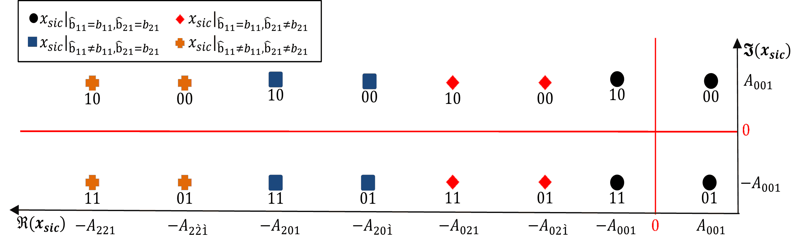
Figure 5: Equivelant constellation of the third user, $N=3$.

Table II presents the four different possible scenarios for this user.

TABLE II: The four possible cases for the third user.

Scenario	$U_{1}$ Detection	$U_{2}$ Detection
$1$	$\checkmark$	$\checkmark$
$2$	$\checkmark$	$\times$
$3$	$\times$	$\checkmark$
$4$	$\times$	$\times$

It should be noted that both $b_{12}$ and $b_{22}$ bits do not affect the error probability of the third user, hence it is assumed that $P_{b_{12}}=P_{b_{22}}=1$. As for the first scenario where $\hat{b}_{11}=b_{11}$ and $\hat{b}_{21}=b_{21}$, the error probability of the third user is derived according to Fig. 5 (solid circles) and (68).

$\boldsymbol{Case}$ $\boldsymbol{1}$: $s_{1}^{(0)}$ $\left(b_{11}^{(0)}\right)$, $\hat{s}_{1}^{(0)}$ $\left(\hat{b}_{11}^{(0)}\right)$, $s_{2}^{(2)}$ $\left(b_{21}^{(1)}\right)$, $\hat{s}_{2}^{(2)}$ $\left(\hat{b}_{21}^{(1)}\right),$ $s_{3}^{(2)}$:

The transmitted signal $x=A_{1\acute{1}\acute{1}}+jA_{111}$ is subtracted by $\hat{s}_{1}$ and $\hat{s}_{2}$, hence, $x_{sic}=A_{00\acute{1}}+jA_{001}$. The error probability for this case can be obtained as follows.

$$P_{b_{31}}|_{\mathbb{A}_{331}}\mathrm{P\!}\left(\hat{b}_{11}^{(0)},\hat{b}_{21}^{(1)}|_{\ddot{\mathbb{A}}_{331}}\right) =\mathrm{P\!}\left(\mathfrak{n}_{3}\geq\alpha_{3}A_{001},\mathfrak{n}_{3}\geq\alpha_{3}A_{\acute{1}11}\right)$$

$$=Q\left(\sqrt{\gamma_{3,11}}\right)$$ (69)

$\mathbb{A}_{331}\rightarrow\left\{b_{11}^{(0)}\text{, }\hat{b}_{11}^{(0)}\text{, }b_{21}^{(1)}\text{, }\hat{b}_{21}^{(1)}\text{, }s_{3}^{(2)}\right\}$, $\ddot{\mathbb{A}}_{331}\rightarrow\left\{b_{11}^{(0)}\text{, }b_{21}^{\left(1\right)}\text{, }s_{3}^{(2)}\right\}$, $\mathfrak{n}_{3}\triangleq\mathfrak{R}\left(\check{w}_{3}\right)$ and $\gamma_{3,11}=\alpha_{3}^{2}A_{001}^{2}/\sigma_{\mathfrak{n}_{3}}^{2}$.

The second bit $b_{32\text{ }}$error probability is derived as follows.

$$P_{b_{32}}|\mathbb{A}_{331}\mathrm{P\!}\left(\hat{b}_{11}^{(0)},\hat{b}_{21}^{(1)}|_{\ddot{\mathbb{A}}_{331}}\right)\!\!\!\!\!\! =\!\!\!\!\!\!\mathrm{P\!}\left(\mathfrak{q}_{3}\leq\alpha_{3}A_{00\acute{1}}\right)\mathrm{P\!}\left(\mathfrak{n}_{3}\geq\alpha_{3}A_{\acute{1}11}\right)$$

$$=\!\!\!\!Q\left(\sqrt{\gamma_{3,11}}\right)\left(1-Q\left(\sqrt{\gamma_{3,1}}\right)\right)\!\!.$$ (70)

where $\mathfrak{q}_{3}\triangleq\mathfrak{I}\left(\check{w}_{3}\right)$.

$\boldsymbol{Case}$ $\boldsymbol{2}$: $s_{1}^{(0)}$ $\left(b_{11}^{(0)}\right)$, $\hat{s}_{1}^{(0)}$ $\left(\hat{b}_{11}^{(0)}\right)$, $s_{2}^{(2)}$ $\left(b_{21}^{(1)}\right)$, $\hat{s}_{2}^{(2)}$ $\left(\hat{b}_{21}^{(1)}\right)$, $s_{3}^{(0)}$:

The error probability of this case is expressed as

$$P_{b_{31}}|_{\mathbb{A}_{332}}\mathrm{P\!}\left(\hat{b}_{11}^{(0)},\hat{b}_{21}^{(1)}|_{\ddot{\mathbb{A}}_{332}}\right) =\mathrm{P\!}\left(\alpha_{3}A_{\acute{1}1\acute{1}}\leq\mathfrak{n}_{3}\leq\alpha_{3}A_{00\acute{1}}\right)$$

$$=Q\left(\sqrt{\gamma_{3,11}}\right)-Q\left(\sqrt{\gamma_{3,2}}\right).$$ (71)

$\mathbb{A}_{332}\rightarrow\left\{b_{11}^{(0)}\text{, }\hat{b}_{11}^{(0)}\text{, }b_{21}^{(1)}\text{, }\hat{b}_{21}^{(1)}\text{, }s_{3}^{(0)}\right\}$ and $\ddot{\mathbb{A}}_{332}\rightarrow\left\{b_{11}^{(0)}\text{, }b_{21}^{(1)}\text{, }s_{3}^{(0)}\right\}$.

For $b_{32\text{ }}$, the error probability can be obtained as

$$P_{b_{32}}|_{\mathbb{A}_{332}}\mathrm{P\!}\left(\hat{b}_{11}^{(0)},\hat{b}_{21}^{(1)}|_{\ddot{\mathbb{A}}_{332}}\right)\!\! =\!\!\mathrm{P\!}\left(\mathfrak{q}_{3}\leq\alpha_{3}A_{00\acute{1}}\right)\mathrm{P\!}\left(\mathfrak{n}_{3}\geq\alpha_{3}A_{\acute{1}1\acute{1}}\right)$$

$$=Q\left(\sqrt{\gamma_{3,11}}\right)\left(1-Q\left(\sqrt{\gamma_{3,2}}\right)\right).$$ (72)

$\boldsymbol{Case}$ $\boldsymbol{3}$: $s_{1}^{(0)}$ $\left(b_{11}^{(0)}\right)$, $\hat{s}_{1}^{(2)}$ $\left(\hat{b}_{11}^{(0)}\right)$, $s_{2}^{(0)}$ $\left(b_{21}^{(0)}\right)$, $\hat{s}_{2}^{(0)}$ $\left(\hat{b}_{21}^{(0)}\right)$, $s_{3}^{(2)}$:

The error probability of this case is derived as

$$P_{b_{32}}|_{\mathbb{A}_{333}}\mathrm{P\!}\left(\hat{b}_{11}^{(0)},\hat{b}_{21}^{(0)}|_{\ddot{\mathbb{A}}_{333}}\right) =\mathrm{P\!}\left(\mathfrak{n}_{3}\geq\alpha_{3}A_{001}\right)$$

$$=Q\left(\sqrt{\gamma_{3,11}}\right).$$ (73)

$\mathbb{A}_{333}\rightarrow\left\{b_{11}^{(0)},\hat{b}_{11}^{(0)},b_{21}^{(0)},\hat{b}_{21}^{(0)},s_{3}^{(2)}\right\}$ and $\ddot{\mathbb{A}}_{333}\rightarrow\left\{b_{11}^{(0)},b_{21}^{(0)},s_{3}^{(2)}\right\}$.

The error probability for $b_{32}$ is

$$P_{b_{32}}|_{\mathbb{A}_{333}}\mathrm{P\!}\left(\hat{b}_{11}^{(0)},\hat{b}_{21}^{(0)}|_{\ddot{\mathbb{A}}_{333}}\right)\!\! =\!\!\mathrm{P\!}\left(\mathfrak{q}_{3}\leq\alpha_{3}A_{00\acute{1}}\right)\mathrm{P\!}\left(\mathfrak{n}_{3}\geq\alpha_{3}A_{\acute{1}\acute{1}1}\right)$$

$$=Q\left(\sqrt{\gamma_{3,11}}\right)\left(1-Q\left(\sqrt{\gamma_{3,3}}\right)\right).$$ (74)

$\boldsymbol{Case}$ $\boldsymbol{4}$: $s_{1}^{(0)}$ $\left(b_{11}^{(0)}\right)$, $\hat{s}_{1}^{(2)}$ $\left(\hat{b}_{11}^{(0)}\right)$, $s_{2}^{(0)}$ $\left(b_{21}^{(0)}\right)$, $\hat{s}_{2}^{(0)}$ $\left(\hat{b}_{21}^{(0)}\right)$, $s_{3}^{(0)}$:

The error probability of this case is obtained as

$$P_{b_{31}}|_{\mathbb{A}_{334}}\mathrm{P\!}\left(\hat{b}_{11}^{(0)},\hat{b}_{21}^{(0)}|_{\ddot{\mathbb{A}}_{334}}\right) =\mathrm{P\!}\left(\mathfrak{n}_{3}\leq\alpha_{3}A_{00\acute{1}}\right)$$

$$\text{ \ \ \ \ \ \ \ \ \ \ \ }-\mathrm{P\!}\left(\mathfrak{n}_{3}\leq\alpha_{3}A_{\acute{1}\acute{1}\acute{1}}\right)$$

$$=Q\left(\sqrt{\gamma_{3,11}}\right)-Q\left(\sqrt{\gamma_{3,4}}\right).$$ (75)

$\mathbb{A}_{334}\rightarrow\left\{s_{1}^{(0)},\hat{s}_{1}^{(2)},s_{2}^{(0)},\hat{s}_{2}^{(0)},s_{3}^{(0)}\right\}$ and $\ddot{\mathbb{A}}_{334}\rightarrow\left\{b_{11}^{(0)},b_{21}^{(0)},s_{3}^{(0)}\right\}$.

For $b_{32}$ is as follows

$$P_{b_{32}}|\mathbb{A}_{334}\mathrm{P\!}\left(\hat{b}_{11}^{(0)},\hat{b}_{21}^{(0)}|_{\ddot{\mathbb{A}}_{334}}\right) =\mathrm{P\!}\left(\mathfrak{q}_{3}\leq\alpha_{3}A_{00\acute{1}}\right)\mathrm{P\!}\left(\mathfrak{n}_{3}\geq\alpha_{3}A_{\acute{1}\acute{1}\acute{1}}\right)$$

$$=Q\left(\sqrt{\gamma_{3,11}}\right)\left(1-Q\left(\sqrt{\gamma_{3,4}}\right)\right).$$ (76)

By taking into consideration the other $60$ cases, $\boldsymbol{Case}$ $\boldsymbol{5}$ to $\boldsymbol{Case}$ $\boldsymbol{64}$, which are obtained in a similar manner, the total BER for the first scenario where $\hat{b}_{11}=b_{11}$ and $\hat{b}_{21}=b_{21}$ can be represented as

$$P_{U_{3}}^{(1)}=\frac{1}{4}Q\left(\sqrt{\gamma_{3,11}}\right)\left(8-\sum_{i=1}^{4}Q\left(\sqrt{\gamma_{3,i}}\right)\right)\\ -\frac{1}{4}\left[Q\left(\sqrt{\gamma_{3,2}}\right)-Q\left(\sqrt{\gamma_{3,4}}\right)\right].$$ (77)

As for the other scenarios, a similar procedure is followed as for the case $\hat{b}_{11}=b_{11}$ and $\hat{b}_{21}=b_{21}$. The analysis for $\hat{b}_{11}=b_{11}$, $\hat{b}_{21}\neq b_{21}$, $\hat{b}_{11}\neq b_{11}$, $\hat{b}_{21}=b_{21}$ and $\hat{b}_{11}\neq b_{11},$ $\hat{b}_{21}\neq b_{21}$ is based on Fig. 5 and (68). The final total BER results for this scenario is respectively given by,

$$P_{U_{3}}^{(2)}=2-Q\left(\sqrt{\gamma_{3,1}}\right)-Q\left(\sqrt{\gamma_{3,2}}\right)-Q\left(\sqrt{\gamma_{3,4}}\right)-Q\left(\sqrt{\gamma_{3,14}}\right)\\ +2Q\left(\sqrt{\gamma_{3,13}}\right)+Q\left(\sqrt{\gamma_{3,11}}\right)\left(4-\sum_{i=1}^{4}Q\left(\sqrt{\gamma_{3,i}}\right)\right)$$ (78)

$$P_{U_{3}}^{(3)}=Q\left(\sqrt{\gamma_{3,11}}\right)\left(\sum_{i=1}^{4}Q\left(\sqrt{\gamma_{3,i}}\right)\right)+Q\left(\sqrt{\gamma_{3,2}}\right)+Q\left(\sqrt{\gamma_{3,4}}\right)$$ (79)

and

$$P_{U_{3}}^{(4)}=Q\left(\sqrt{\gamma_{3,1}}\right)-Q\left(\sqrt{\gamma_{3,15}}\right)+\sum_{i=16}^{18}Q\left(\sqrt{\gamma_{3,i}}\right)\\ +Q\left(\sqrt{\gamma_{3,11}}\right)\left(\sum_{i=1}^{4}Q\left(\sqrt{\gamma_{3,i}}\right)\right)$$ (80)

where $\gamma_{3,12}=\alpha_{3}^{2}A_{02\acute{1}}^{2}/\sigma_{\mathfrak{n}_{3}}^{2}$, $\gamma_{3,13}=\alpha_{3}^{2}A_{201}^{2}/\sigma_{\mathfrak{n}_{3}}^{2}$, $\gamma_{3,14}=\alpha_{3}^{2}A_{20\acute{1}}^{2}/\sigma_{\mathfrak{n}_{3}}^{2}$, $\gamma_{3,15}=\alpha_{3}^{2}A_{2\grave{2}\acute{1}}^{2}/\sigma_{\mathfrak{n}_{3}}^{2}$, $\gamma_{3,16}=\alpha_{3}^{2}A_{2\grave{2}1}^{2}/\sigma_{\mathfrak{n}_{3}}^{2}$, $\gamma_{3,17}=\alpha_{3}^{2}A_{22\acute{1}}^{2}/\sigma_{\mathfrak{n}_{3}}^{2}$, $\gamma_{3,18}=\alpha_{3}^{2}A_{221}^{2}/\sigma_{\mathfrak{n}_{3}}^{2}$. By combining the results in (77), (78), (79) and (80), the total BER for the third user can be computed as

$$P_{U_{3}}=\frac{1}{4}\left[\left(\sum_{i}v_{i}Q\left(\sqrt{\gamma_{3,i}}\right)\right)\right]\text{,}\\ \text{ }i=\left[2,4,11,13,14,15,16,17,18\right]\text{,}\\ \mathbf{v}=[-1,-1,12,2,-1,-1,-1,-1,-1].$$ (81)

IV-D Average BER, $N=3$

Similar to the $N=2$ NOMA system, the average BER of $N=3$ NOMA system can be evaluated by averaging over the PDFs of all $\gamma_{n,c}$ values, which are given in Appendix I. Therefore, by substituting $N=3$ and $n=\left[1,2,3\right]$ in the ordered PDF in  (93), the exact average BER of the first and second users can be simplified to

$$\bar{P}_{U_{1}}=\frac{3}{4\pi\Gamma(m)}\sum\limits_{c=1}^{4}\sum_{k=0}^{2}\sum_{i=0}^{\infty}\binom{2}{k}\left(-1\right)^{k}S_{i}\left(\frac{m}{\overline{\gamma}_{1,c}}\right)^{m(1+k)}\\ \times\int_{0}^{\frac{\pi}{2}}\frac{\left(i+mk\right)!}{\left(\frac{1}{2\sin^{2}\left(\psi_{1,c}\right)}+\frac{m\text{ }\left(1+k\right)}{\overline{\gamma}_{1,c}}\right)^{i+mk+1}}d\psi_{1,c}$$ (82)

$$\bar{P}_{U_{2}}=\frac{3}{2\pi\Gamma(m)}\sum\limits_{c=1}^{10}\sum_{k=0}^{1}\sum_{i=0}^{\infty}\left(-1\right)^{k}S_{i}g_{c}\left(\frac{m}{\overline{\gamma}_{2,c}}\right)^{m(2+k)}\\ \times\int_{0}^{\frac{\pi}{2}}\frac{\left(i+m(1+k)\right)!}{\left(\frac{1}{2\sin^{2}\left(\psi_{2,c}\right)}+\frac{m\text{ }\left(2+k\right)}{\overline{\gamma}_{2,c}}\right)^{i+m(1+k)+1}}d\psi_{2,c}\text{,}\\ \mathbf{g}=\left[1,1,-1,-1,6,2,-1,-1,1,1\right]$$ (83)

and

$$\bar{P}_{U_{3}}=\frac{3}{8\pi\Gamma(m)}\sum\limits_{c=1}^{18}\sum_{i=0}^{\infty}v_{c}S_{i}\left(\frac{m}{\overline{\gamma}_{3,c}}\right)^{3m}\\ \times\int_{0}^{\frac{\pi}{2}}\frac{\left(i+2m\right)!}{\left(\frac{1}{2\sin^{2}\left(\psi_{3,c}\right)}+\frac{3m\text{ }}{\overline{\gamma}_{3,c}}\right)^{i+2m+1}}d\psi_{3,c}\text{,}\\ c\in\left\{2,4,11,13,14,15,16,17,18\right\}\text{,}\\ \mathbf{v}=[-1,-1,12,2,-1,-1,-1,-1,-1].$$ (84)

The closed-form average BER for the first, second, and third users over Rayleigh fading channel $\left(m=1\right)$ are shown in (85), (86), and (87), respectively.

$$\bar{P}_{U_{1}}=\frac{1}{4}\mathop{\displaystyle\sum}\limits_{c=1}^{4}\left(1-\sqrt{\frac{2\overline{\gamma}_{{}_{3,c}}}{2\overline{\gamma}_{3,c}+3}}\right)$$ (85)

$$\bar{P}_{U_{2}}=\frac{1}{4}\left[\mathop{\displaystyle\sum}\limits_{c=1}^{10}g_{c}\left(\sqrt{\frac{2\overline{\gamma}_{3,c}}{2\overline{\gamma}_{3,c}+3}}-\frac{3}{2}\sqrt{\frac{\overline{\gamma}_{3,c}}{\overline{\gamma}_{3,c}+1}}+\frac{1}{2}\right)\right]\text{,}\\ \mathbf{g}=\left[1,1,-1,-1,6,2,-1,-1,1,1\right]$$ (86)

and

$$\bar{P}_{U_{3}}=\frac{1}{4}\sum_{c}v_{c}\left(-\sqrt{\frac{2\overline{\gamma}_{3,c}}{2\overline{\gamma}_{3,c}+3}}-3\sqrt{\frac{2\overline{\gamma}_{3,c}}{2\overline{\gamma}_{3,c}+1}}\right.\\ +\left.3\sqrt{\frac{\overline{\gamma}_{3,c}}{\overline{\gamma}_{3,c}+1}}+\frac{1}{2}\right)\\ c\in\left\{2,4,11,13,14,15,16,17,18\right\},\\ \mathbf{v}=[-1,-1,12,2,-1,-1,-1,-1,-1].$$ (87)

V Optimum Power Allocation Problem

The optimal power allocation problem is formulated for two different objective functions using the derived exact BER expressions for $N=2$ and $N=3$ NOMA systems. The first objective is to obtain the optimum power coefficients $\ddot{\beta}_{n}$ that minimize the overall average BER of all users. The second objective function is to evaluate the optimum power coefficients which guarantee fairness among all users. The fairness in this work indicates equal BER for all the users.

The optimal power allocation for minimizing the average BER is formulated as follows:

$$\min_{\beta_{n}}\text{ }\frac{1}{N}\sum_{n=1}^{N}\bar{P}_{U_{n}}$$ (88a)

subject to:

$$\sum_{n=1}^{N}\beta_{n}=1$$ (88b)

$$\beta_{l}\geqslant\beta_{k}\text{, }l\neq k\text{, }l<k\text{, }\left\{l,k\right\}\in\left\{1,2,\ldots,N\right\}$$ (88c)

where the first constraint limits the maximum transmit power, which is normalized to unity. The second constraint is used assure that the power allocated to each user is inversely proportional to its channel gain, i.e., $$\beta_{1}>\beta_{2}>\cdots>\beta_{N} \alpha_{1}<\alpha_{2}<\cdots<\alpha_{N}$$ are assigned for the users with the channel gains , respectively. The problem in (88b) is a constrained non-linear optimization problem which is solved using the Interior-Point Optimization (IPO) algorithm [29].

The optimal power allocation for achieving fairness among the users in the NOMA system is formulated as follows:

$$\bar{P}_{U_{l}}=\bar{P}_{U_{k}}\text{, }\forall\{l,k\}\in\left\{1,2,\ldots,N\right\}\text{, }l\neq k$$ (89)

The constraints for the second optimization problem are similar to those in the first optimization problem and the solution can be obtained using the same approach.

VI Numerical and Simulation Results

This section presents numerical and Monte Carlo simulation results for $N=2$ and $N=3$ downlink NOMA systems. All users are assumed to be equipped with a single antenna, and the channel between the BS and each user is modeled as an ordered Nakagami-$m$ flat fading channel. The randomly generated channels are ordered based on their strength, where the weakest channel is assigned to the first user and the strongest channel is assigned to $N$th user. The transmitted symbols for all users are selected uniformly from a Gray coded QPSK constellation. The total transmit power from the BS is unified for all cases, $P_{T}=1$.

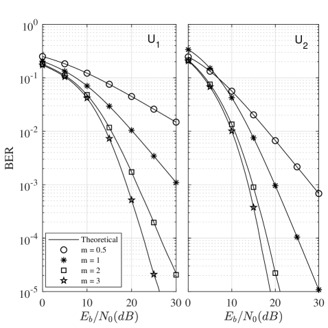
Figure 6: BER for the first and second users, $N=2$, $m=0.5,1,2$ and $3$, and $\Omega=1.$

Fig. 6 presents the analytical and simulated BER performance of the two users scenario, $N=2$ for power coefficients $\beta_{1}=0.7$ and $\beta_{2}=0.3$, $\Omega=1$ and various values of $m$ over a range of $E_{b}/N_{0}$, where $E_{b}/N_{0}=1/N_{0}$. As can be noted from the figure, the analytical results obtained using (36), (37), (38), and (39) perfectly match the simulation results for all the considered values of $m$ and $E_{b}/N_{0}$. It is worth noting that the $m=1$ case corresponds to the derived to the Rayleigh fading case.

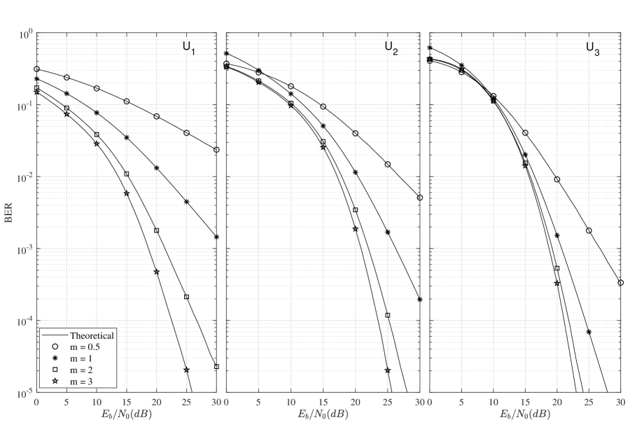
Figure 7: BER for the first, second, and third users in the $N=2$, $m=0.5,1,2$ and $3$, and $\Omega=1.$

Fig. 7 is generally similar to Fig. 6, except that it considers the three users scenario, i.e., $N=3$. The power allocation coefficients are $\beta_{1}=0.8$, $\beta_{2}=0.15$ and $\beta_{3}=0.05$. The figure clearly shows the perfect match between the analytical results obtained using (82)-(87) and simulation results for all $m$ values and over the entire $E_{b}/N_{0}$ range. As can be seen from Figures 6 and 7, the performance of the first user is more sensitive to the variations of $m$ as compared to the second and third users, which is due to the fact that the fading effect becomes less significant for the near users.

Figure 8: Exact BER and union bound for the first and second users, $N=2$, $m=1$ and $\Omega=1.$

Fig. 8 compares the exact BER and union bound [21] for $N=2$, $m=1$, $\beta_{1}=0.7$ and $\beta_{2}=0.3$. It can be noted that the union bound is generally tight in the high $E_{b}/N_{0}$ range, particularly for the second user. For example, the gap between the exact BER and union bound at $E_{b}/N_{0}=20$ dB is about $2$ dB for the first user and $1$ dB for the second user. At low $E_{b}/N_{0}$, the gap may increase to $3$ dB. Therefore, using the exact BER expression is critical when accurate BER estimates are desired.

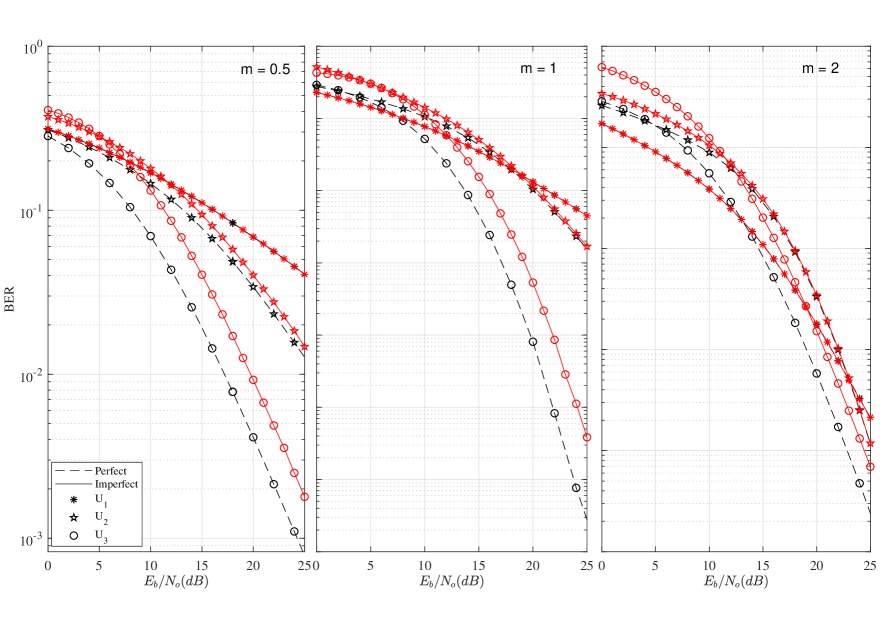
Figure 9: Perfect and imperfect BER for the first, second, and third users in the N=3, $m=0.5,1$ and $2$, and $\Omega=1$.

Fig. 9 shows the BER for $N=3$ under perfect and imperfect SIC for different values of $m$. Although the perfect SIC assumption may tremendously reduce the BER analysis, the results presented in Fig. 9 show that such assumption is too optimistic, particularly for $U_{3}$. As expected, the results for $U_{1}$ with/without SIC are identical because $U_{1}$ detection does not involve a SIC process. For $U_{2}$, the impact of the perfect SIC assumption is apparent at low SNRs, because at high $E_{b}/N_{0}$, $U_{1}$ signal is mostly detected correctly, and thus, the results with/without SIC converge. The third user $U_{3}$ is the one who will experience the maximum difference because the probability that the two SIC operations are performed successfully is relatively small. Therefore, the BER with and without SIC for $U_{3}$ will exhibit substantial difference. Moreover, as $m$ increases, the BER with perfect and imperfect BERs become closer, particularly at high SNRs, which is due to that fact that for high values of $m$ the fading is less severe, which implies that the probability of having successful SIC operations is higher as compared to the low $m$ values.

Tables III and IV present the optimal power coefficients that provide equal BER for all users. The results are obtained for different values of $E_{b}/N_{0}$, $N=2$, $3$, and $m=1$, $3$. As can be noted from the results in Table III, most of the power is actually allocated for $U_{1}$, particularly at high SNRs. For $N=2$, the first user is allocated more than $98\%$ of the total power at $E_{b}/N_{0}=30$ dB, and it is about $89\%$ for $N=3$. Moreover, the range of values that the power coefficients might be allocated depends drastically on $N$. The same trends can be noted for the $m=3$ case in Table IV. Nevertheless, the power given to the first user generally decreases by increasing $m$ as the impact of the AWGN becomes more noticeable.

TABLE III: Optimal power allocation to achieve fairness, for $m=1$.

	$N=2$		$N=3$
$E_{b}/N_{0}$	$\beta_{1}$	$\beta_{2}$	$\beta_{1}$	$\beta_{2}$	$\beta_{3}$
$0$	$0.838$	$0.186$	$0.500$	$0.27$	$0.23$
$10$	$0.851$	$0.151$	$0.790$	$0.114$	$0.095$
$20$	$0.916$	$0.083$	$0.818$	$0.151$	$0.029$
$30$	$0.981$	$0.018$	$0.890$	$0.095$	$0.014$

TABLE IV: Optimal power allocation to achieve fairness, for $m=3$.

	$N=2$		$N=3$
$E_{b}/N_{0}$	$\beta_{1}$	$\beta_{2}$	$\beta_{1}$	$\beta_{2}$	$\beta_{3}$
$0$	$0.830$	$0.17$	$0.490$	$0.24$	$0.27$
$10$	$0.841$	$0.159$	$0.700$	$0.201$	$0.099$
$20$	$0.903$	$0.097$	$0.806$	$0.145$	$0.049$
$30$	$0.962$	$0.038$	$0.850$	$0.088$	$0.062$

Table V shows the optimal power coefficients which minimize the average BER for $N=2$, $3$, and $m=1$. As can be noted from the table, the power allocation should be performed meticulously to achieve the desire results. Although the exact results are different, the observations about the power coefficients generally follows those of the BER fairness case. Moreover, the optimum power allocation requires the knowledge of  the $E_{b}/N_{0}$ at the transmitter. For example, the value of $\beta_{2}$ drops by about $50\%$ when the $E_{b}/N_{0}$ is increased from $20$ to $30$ dB.

TABLE V: Optimal power allocation to achieve minimum average BER, $m=1$.

	$N=2$		$N=3$
$E_{b}/N_{0}$	$\beta_{1}$	$\beta_{2}$	$\beta_{1}$	$\beta_{2}$	$\beta_{3}$
$0$	$0.810$	$0.189$	$0.546$	$0.320$	$0.132$
$10$	$0.842$	$0.157$	$0.670$	$0.273$	$0.057$
$20$	$0.896$	$0.103$	$0.860$	$0.116$	$0.023$
$30$	$0.943$	$0.056$	$0.946$	$0.046$	$0.007$

Figure 10: The average BER for $N=2$ and $N=3$ for two different power levels and the minimum value, $m=1.$

Fig. 10 presents the BER using the optimum power coefficients that guarantees minimizing the average BER, in addition, two other curves obtained using fixed power values are used where $\beta_{1}=0.7$, and $0.9$ for $N=2$, and $\left\{\beta_{1}=0.84\text{, }\beta_{2}=0.12\right\}$, and $\left\{\beta_{1}=0.9,\beta_{2}=0.07\right\}$ for $N=3$. As can be noted from the figure, allocating the power coefficients appropriately might save the need to use adaptive power values. On the other hand, large deviations from the optimum power values might result in severe BER degradation.

Figure 11: BER for the first, and second users at various $m$ values, $\Omega=1$, $N=2$ NOMA system.

Figure 12: BER for the first, second, and third users at various $m$ values, $\Omega=1$ and $N=3$.

Figures 11 and 12 show the effect of the fading factor on the performance of each user for NOMA systems with $N=2$, $3$ where $E_{b}/N_{0}=10,$ and $18$ dB. Power allocation coefficients at $E_{b}/N_{0}=10$ dB are assigned as follows, $\beta_{1}=0.84,$ $\beta_{2}=0.16$ and $\beta_{1}=0.67,$ $\beta_{2}=0.27,$ and $\beta_{3}=0.06$ for the two and three users’ systems, respectively. For the case where $E_{b}/N_{0}=18$ dB, the power allocation coefficients are $\beta_{1}=0.88,$ $\beta_{2}=0.12$ and $\beta_{1}=0.84,$ $\beta_{2}=0.13,$ and $\beta_{3}=0.03$ for the two and three users’ systems, respectively. It should be noted that the power allocation coefficients are the optimal values that minimize the average BER. As can be seen from Figures 11 and  12, the BER performance of all users highly depends on the fading parameter $m$. Additionally, it is shown that $m$ affects the performance of the higher order users more than the lower order users, which is due to the ordering of users based on the channel conditions that resulted in an enhanced performance for higher order users. Moreover, when $E_{b}/N_{0}$ increases, the effect of $m$ on the performance increases because the BER will be mostly determined by  the fading.

VII Conclusion

This work presented the performance of a downlink NOMA system in terms of BER where exact BER expressions were derived for different users over Nakagami-$m$ fading channels for two and three users’ scenarios, where imperfect SIC is considered. The BER can be evaluated numerically for general $m$ values, as one of the integrals does not have an analytical solution. For the special case of Rayleigh fading, $m=1$, closed-form expressions are derived for several cases of interest. Moreover, constrained nonlinear optimization problems which aim to find the optimum power coefficients that minimize the average BER and achieve fairness among the users were formulated. Each objective can be used for different purposes, for example, if the main goal of NOMA system is to fairly acquire equal average BER for all users such as satellite systems, then the fairness optimal power allocation should be evaluated. On the other hand, when the purpose of a NOMA system is to minimize the overall average BER for applications such as , then the latter problem formulation can be used.

Appendix I: Average BER over Nakagami-$m$ Fading Channel

The average BER for a NOMA system over Nakagami-$m$ fading channel follows the order statistics of Nakagami-$m$ distribution. Based on order statistics theory, the general ordered PDF of the channel gain of the $n$th user can be expressed as [30],

$$f_{n}\left(\alpha_{n}\right)=K_{n}f\left(\alpha_{n}\right)\left[F\left(\alpha_{n}\right)\right]^{n-1}\left[1-F\left(\alpha_{n}\right)\right]^{N-n}$$ (90)

where $K_{n}=\frac{N!}{\left(n-1\right)!\left(N-n\right)!}$, $f\left(\alpha_{n}\right)$ and $F\left(\alpha_{n}\right)$ are respectively the PDF and CDF of Nakagami-$m$ distribution with parameters $m$ and $\Omega$,

$$f(\alpha_{n})=\frac{2m^{m}\alpha_{n}^{2m-1}}{\Omega^{m}\Gamma\left(m\right)}\mathrm{e}^{\left(-\frac{m\alpha_{n}^{2}}{\Omega}\right)}$$ (91)

$$F(\alpha_{n})=\frac{1}{\Gamma\left(m\right)}\Phi\left(m,\frac{m\alpha_{n}^{2}}{\Omega}\right)$$ (92)

where $\Gamma(m)$ is the upper incomplete Gamma function, $\Omega=\mathbb{E}\left(\alpha_{n}^{2}\right)$, $m=\frac{\Omega^{2}}{Var\left(\alpha_{n}^{2}\right)}$, and $\Phi\left(a,z\right)=\mathop{\displaystyle\int}_{0}^{z}t^{a-1}\mathrm{e}^{-t}dt$ is the lower incomplete Gamma function [31]. Therefore, the ordered PDF of the $n$th channel gain over Nakagami-$m$ channel is

$$f_{n}(\alpha_{n})=\frac{2K_{n}m^{m}\alpha_{n}^{2m-1}}{\Omega^{m}\left[\Gamma\left(m\right)\right]^{n}}\mathrm{e}^{\left(-\frac{m\alpha_{n}^{2}}{\Omega}\right)}\left[\Phi\left(m,\frac{m\alpha_{n}^{2}}{\Omega}\right)\right]^{n-1}\\ \times\left[1-\frac{\Phi\left(m,\frac{m\alpha_{n}^{2}}{\Omega}\right)}{\Gamma\left(m\right)}\right]^{N-n}.$$ (93)

Because the lower incomplete Gamma function is raised to a power, rendering the integral analytically for $m>1$ is intractable. Therefore, the infinite series representation of the lower incomplete Gamma function can be used [32],

$$\left[\Phi\left(m,\frac{m\alpha_{n}^{2}}{\Omega}\right)\right]^{\mu}=\left(\frac{m\alpha_{n}^{2}}{\Omega}\right)^{m\mu}\left[\Gamma\left(m\right)\right]^{\mu}\mathrm{e}^{-\frac{\mu m\alpha_{n}^{2}}{\Omega}}\sum_{i=0}^{\infty}S_{i}\alpha_{n}^{2i}$$ (94)

where

$$S_{i}=\left\{\begin{array}[]{lc}a_{0}^{\mu}\text{,}&i=0\\ \frac{1}{ia_{0}}\mathop{\displaystyle\sum}\limits_{z=1}^{i}\left(z\left(\mu+1\right)-i\right)a_{z}S_{i-z}\text{, }&i\neq 0\end{array}\right.\text{, }\\ a_{{}_{z}}=\frac{\left(\frac{m}{\Omega}\right)^{z}}{\Gamma(m+z+1)}\text{, }z=0,1,...,\infty.$$ (95)

In addition, the term $\left[1-\frac{\Phi\left(m,\frac{m\alpha_{n}^{2}}{\Omega}\right)}{\Gamma\left(m\right)}\right]^{N-n}$is expanded using binomial theorem [33]

$$\left[1-\frac{\Phi\left(m,\frac{m\alpha_{n}^{2}}{\Omega}\right)}{\Gamma\left(m\right)}\right]^{N-n}=\sum_{k=0}^{N-n}\binom{N-n}{k}\left(\frac{-\Phi\left(m,\frac{m\alpha_{n}^{2}}{\Omega}\right)}{\Gamma\left(m\right)}\right)^{k}.$$ (96)

Now, $\gamma_{n,c}$ for a Nakagami-$m$ channel follows the Gamma distribution $\mathcal{G}\left(k,\theta\right)$ where $k=m$, and $\theta=\frac{\Omega}{m}$, with the following PDF and CDF

$$f(\gamma_{n,c})=\frac{m^{m}\gamma_{n,c}^{m-1}}{\overline{\gamma}_{n,c}^{m}\Gamma(m)}\mathrm{e}^{-\frac{m_{n}\gamma_{n,c}}{\bar{\gamma}_{n,c}}}$$ (97)

and

$$F\left(\gamma_{n,c}\right)=\frac{\Phi\left(m,\frac{m\gamma_{n,c}}{\overline{\gamma}_{n,c}}\right)}{\Gamma(m)}$$ (98)

respectively, where $\overline{\gamma}_{n,c}=A_{u_{2}u_{2}u_{3}}^{2}\Omega/\sigma_{n}^{2}$ and $c$ is the index parameter.

The ordered PDF of $\gamma_{n,c}$ of the $n$th channel can be expressed using (90), (94), and (97), as follows

$$f_{n}(\gamma_{n,c})=\frac{K_{n}}{\Gamma(m)}\sum_{k=0}^{N-n}\binom{N-n}{k}\left(-1\right)^{k}\mathrm{e}^{-\frac{m\text{ }\gamma_{{}_{n,c}}}{\overline{\gamma}_{n,c}}\left(n+k\right)}\\ \times\left(\frac{m}{\overline{\gamma}_{n,c}}\right)^{m(n+k)}\sum_{i=0}^{\infty}S_{i}\gamma_{{}_{n,c}}^{i+m(n+k-1)}.$$ (99)

In order to evaluate the average BER of the $n$th user over Nakagami-$m$ channel, (99) and the alternative representation of the $Q$ function defined by [34] are utilized. Moreover, the following integral is used [33],

$$\int_{0}^{\infty}x^{t}\mathrm{e}^{-bx}dx=\frac{t!}{b^{t+1}}\text{, \ \ }t\in\left\{0,1,\ldots,b\right\}>0.$$ (100)

The general average BER for user $n$ is given by,

$$\overline{P}_{U_{n}} =\int_{0}^{\infty}Q\left(\gamma_{n,c}\right)f_{n}\left(\gamma_{n,c}\right)d\gamma_{n,c}$$

$$=\frac{K_{n}}{\pi\Gamma(m)}\int\limits_{0}^{\infty}\int\limits_{0}^{\frac{\pi}{2}}\frac{1}{\mathrm{e}^{\frac{\gamma_{n,c}}{2\sin^{2}\left(\psi_{n,c}\right)}}}\sum_{k=0}^{N-n}\tbinom{N-n}{k}\frac{\left(-1\right)^{k}}{\mathrm{e}^{\frac{m\text{ }\gamma_{{}_{n},c}}{\overline{\gamma}_{n,c}}\left(n+k\right)}}$$

$$\text{ \ \ \ \ \ \ \ }\times\left(\frac{m}{\overline{\gamma}_{n,c}}\right)^{m(n+k)}\sum_{i=0}^{\infty}S_{i}\gamma_{{}_{n,c}}^{i+m(n+k-1)}d\psi_{n,c}d\gamma_{n,c}$$

$$=\frac{K_{n}}{\pi\Gamma(m)}\sum_{k=0}^{N-n}\sum_{i=0}^{\infty}\tbinom{N-n}{k}\left(-1\right)^{k}S_{i}\frac{m^{m(n+k)}}{\overline{\gamma}_{n,c}^{m(n+k)}}$$

$$\text{ \ \ \ \ \ \ }\times\int\limits_{0}^{\frac{\pi}{2}}\frac{\left[i+m(n+k-1)\right]!}{\left(\frac{1}{2\sin^{2}\left(\psi_{n,c}\right)}+\frac{m\text{ }\left(n+k\right)}{\overline{\gamma}_{n,c}}\right)^{i+m(n+k-1)+1}}d\psi_{n,c}.$$ (101)

Although the integral in (101) does not have an analytical solution, it can be easily solved numerically.

Tasneem Assaf (S’14) received the B.Sc. degree in communications engineering from Khalifa University (KU), Abu Dhabi, UAE, in 2014, and the master’s degree in electrical engineering from the American University of Sharjah (AUS), Sharjah, UAE, in 2016. She is currently pursuing the Ph.D. degree from KU. Her research interests include smart grids, optimization, wireless communications, and machine learning.

Arafat Al-Dweik (S’97-M’01-SM’04) received the M.S. (Summa Cum Laude) and Ph.D. (Magna Cum Laude) degrees in electrical engineering from Cleveland State University, Cleveland, OH, USA in 1998 and 2001, respectively. He was with Efficient Channel Coding, Inc., Cleveland-Ohio, from 1999 to 2001. From 2001 to 2003, he was the Head of Department of Information Technology at the Arab American University in Palestine. Since 2003, he is with the Department of Electrical Engineering, Khalifa University, United Arab Emirates. He joined University of Guelph, ON, Canada, as an Associate Professor from 2013-2014. Dr. Al-Dweik is a Visiting Research Fellow at the School of Electrical, Electronic and Computer Engineering, Newcastle University, Newcastle upon Tyne, UK and he is Research Professor Western University, London, ON, Canada and University of Guelph. Dr Al-Dweik has extensive editorial experience where he served as an Associate Editor at the IEEE Transactions on Vehicular Technology and the IET Communications. Dr Al-Dweik has extensive research experience in various areas of wireless communications that include modulation techniques, channel modeling and characterization, synchronization and channel estimation techniques, OFDM technology, error detection and correction techniques, MIMO and resource allocation for wireless networks. Dr. Al-Dweik is a member of Tau Beta Pi and Eta Kappa Nu. He was awarded the Fulbright scholarship from 1997 to 1999. He received the Hijjawi Award for Applied Sciences in 2003 and the Fulbright Alumni Development Grant in 2003 and 2005, and the Dubai Award for Sustainable Transportation in 2016. He is a Senior Member of the IEEE, and a Registered Professional Engineer in the Province of Ontario, Canada.

Mohamed El Moursi (M’12, SM15) received the B.Sc. and M.Sc. degrees from Mansoura University, Mansoura, Egypt, in 1997 and 2002, respectively, and the Ph.D. degree from the University of New Brunswick (UNB), Fredericton, NB, Canada, in 2005, all in electrical engineering. He was a Research and Teaching Assistant in the Department of Electrical and Computer Engineering, UNB, from 2002 to 2005. He joined McGill University as a Postdoctoral Fellow with the Power Electronics Group. He joined Vestas Wind Systems, Arhus, Denmark, in the Technology R&D with the Wind Power Plant Group. He was with TRANSCO, UAE, as a Senior Study and Planning Engineer. He is currently a Professor in the Electrical and Computer Engineering Department at Khalifa University of Science and Technology- Masdar Campus and seconded to a Professor Position in the Faculty of Engineering, Mansoura University, Mansoura, Egypt and currently on leave. He was a Visiting Professor at Massachusetts Institute of Technology, Cambridge, Massachusetts, USA. Dr. Shawky is currently an Editor of IEEE Transactions on Power Delivery, IEEE Transactions on Power Systems, Associate Editor of IEEE Transactions on Power Electronics, Guest Editor of IEEE Transactions on Energy Conversion, Guest Editor-in-Chief for special section between TPWRD and RPWRS, Editor for IEEE Power Engineering Letters, Regional Editor for IET Renewable Power Generation and Associate Editor for IET Power Electronics Journals. His research interests include power system, power electronics, FACTS technologies, VSC-HVDC systems, Microgrid operation and control, Renewable energy systems (Wind and PV) integration and interconnections.

Hatem Zeineldin (M’06–SM’13) received the B.Sc. and M.Sc. degrees in electrical engineering from Cairo University, Giza, Egypt, in 1999 and 2002, respectively, and the Ph.D. degree in electrical and computer engineering from the University of Waterloo, Waterloo, ON, Canada, in 2006. He was with Smith and Andersen Electrical Engineering, Inc., North York, ON, USA, where he was involved in projects involving distribution system designs, protection, and distributed generation. He was a Visiting Professor with the Massachusetts Institute of Technology, Cambridge, MA, USA. He is currently a Professor with the Khalifa University of Science and Technology, Abu Dhabi, UAE, and is currently on leave from the Faculty of Engineering, Cairo University, Giza. His current research interests include distribution system protection, distributed generation, and micro grids. He is currently an Editor for the IEEE Transactions on Energy Conversion and the IEEE Transactions on Smart Grid.

References

- [1] S. Mattisson, “An overview of 5G requirements and future wireless networks: Accommodating scaling technology,” IEEE Solid-State Circuits Mag., vol. 10, no. 3, pp. 54–60, May 2018.
- [2] L. Bariah, S. Muhaidat, and A. Al-Dweik, “Error probability analysis of NOMA-based relay networks with SWIPT,” IEEE Commun. Lett., vol. 23, no. 7, pp. 1223–1226, Jul. 2019.
- [3] E. Hossain and M. Hasan, “5G cellular: key enabling technologies and research challenges,” IEEE Instrum. Meas. Mag., vol. 18, no. 3, pp. 11–21, Jun. 2015.
- [4] M. Kalil, A. Al-Dweik, M. F. Abu Sharkh, A. Shami, and A. Refaey, “A framework for joint wireless network virtualization and cloud radio access networks for next generation wireless networks,” IEEE Access, vol. 5, pp. 20 814–20 827, 2017.
- [5] M. Kalil, A. Moubayed, A. Shami, and A. Al-Dweik, “Efficient low-complexity scheduler for wireless resource virtualization,” IEEE Wireless Commun. Lett., vol. 5, no. 1, pp. 56–59, Feb. 2016.
- [6] Q. Nadeem, A. Kammoun, M. Debbah, and M. Alouini, “Design of 5G full dimension massive MIMO systems,” IEEE Trans. Commun., vol. 66, no. 2, pp. 726–740, Feb. 2018.
- [7] H. Mukhtar, A. Al-Dweik, and A. Shami, “Turbo product codes: Applications, challenges, and future directions,” IEEE Commun. Surveys Tuts., vol. 18, no. 4, pp. 3052–3069, 4th Quart. 2016.
- [8] L. Dai, B. Wang, Z. Ding, Z. Wang, S. Chen, and L. Hanzo, “A survey of non-orthogonal multiple access for 5G,” IEEE Commun. Surveys Tuts., vol. 20, no. 3, pp. 2294–2323, 3rd Quart. 2018.
- [9] S. M. R. Islam, N. Avazov, O. A. Dobre, and K. Kwak, “Power-domain non-orthogonal multiple access (NOMA) in 5G systems: Potentials and challenges,” IEEE Commun. Surveys Tuts, vol. 19, no. 2, pp. 721–742, 2nd Quart. 2017.
- [10] J. Ding, J. Cai, and C. Yi, “An improved coalition game approach for MIMO-NOMA clustering integrating beamforming and power allocation,” IEEE Trans. Veh. Technol., vol. 68, no. 2, pp. 1672–1687, Feb. 2019.
- [11] M. Al-Imari, M. A. Imran, R. Tafazolli, and D. Chen, “Subcarrier and power allocation for LDS-OFDM system,” in Proc. IEEE Veh. Technol. Conf. (VTC), May 2011, pp. 1–5.
- [12] F. Kara and H. Kaya, “On the error performance of cooperative-NOMA with statistical CSIT,” IEEE Commun. Lett., vol. 23, no. 1, pp. 128–131, Jan. 2019.
- [13] Z. Tang, J. Wang, J. Wang, and J. Song, “On the achievable rate region of NOMA under outage probability constraints,” IEEE Commun. Lett., vol. 23, no. 2, pp. 370–373, Feb. 2019.
- [14] Q. Sun, S. Han, C. I, and Z. Pan, “On the ergodic capacity of MIMO NOMA systems,” IEEE Wireless Commun. Lett., vol. 4, no. 4, pp. 405–408, Aug. 2015.
- [15] L. Yao, J. Mei, H. Long, L. Zhao, and K. Zheng, “A novel multi-user grouping scheme for downlink non-orthogonal multiple access systems,” in Proc. IEEE Wireless Commun. Netw. Conf., Apr. 2016, pp. 1–6.
- [16] F. Liu, P. Mahõnen, and M. Petrova, “Proportional fairness-based power allocation and user set selection for downlink NOMA systems,” in Proc. Conf. Commun. (ICC), May 2016, pp. 1–6.
- [17] Z. Ding, F. Adachi, and H. V. Poor, “The application of MIMO to non-orthogonal multiple access,” IEEE Trans. Wireless Commun., vol. 15, no. 1, pp. 537–552, Jan. 2016.
- [18] C. Park, H. Lee, and J. Lim, “Capacity and fairness trade-off in an outage situation over multiuser diversity systems,” IEEE Commun. Lett., vol. 15, no. 2, pp. 184–186, Feb. 2011.
- [19] Z. Ding, P. Fan, and H. V. Poor, “Impact of user pairing on 5G nonorthogonal multiple-access downlink transmissions,” IEEE Trans. Veh. Technol., vol. 65, no. 8, pp. 6010–6023, Aug. 2016.
- [20] M. B. Shahab, M. F. Kader, and S. Y. Shin, “On the power allocation of non-orthogonal multiple access for 5G wireless networks,” in Proc. Int. Conf. Open Source Syst. Technol. (ICOSST), Dec. 2016, pp. 89–94.
- [21] L. Bariah, S. Muhaidat, and A. Al-Dweik, “Error probability analysis of non-orthogonal multiple access over nakagami- fading channels,” IEEE Trans. Commun., vol. 67, no. 2, pp. 1586–1599, Feb. 2019.
- [22] F. Kara and H. Kaya, “Performance analysis of SSK-NOMA,” IEEE Trans. Veh. Technol., vol. 68, no. 7, pp. 6231 – 6242, May 2019.
- [23] Q. He, Y. Hu, and A. Schmeink, “Closed-form symbol error rate expressions for non-orthogonal multiple access systems,” IEEE Trans. Veh. Technol., vol. 68, no. 7, pp. 6775 – 6789, Jul. 2019.
- [24] I. Lee and J. Kim, “Average symbol error rate analysis for non-orthogonal multiple access with M-ary QAM signals in rayleigh fading channels,” IEEE Commun. Lett., pp. 1–1, Jun. 2019.
- [25] X. Wang, F. Labeau, and L. Mei, “Closed-form BER expressions of QPSK constellation for uplink non-orthogonal multiple access,” IEEE Commun. Lett., vol. 21, no. 10, pp. 2242–2245, Oct. 2017.
- [26] H. Haci, H. Zhu, and J. Wang, “Performance of non-orthogonal multiple access with a novel asynchronous interference cancellation technique,” IEEE Trans. Commun., vol. 65, no. 3, pp. 1319–1335, Mar. 2017.
- [27] F. Kara and H. Kaya, “BER performances of downlink and uplink NOMA in the presence of SIC errors over fading channels,” IET Commun., vol. 12, no. 15, pp. 1834–1844, Sep. 2018.
- [28] J. G. Proakis and M. Salehi, Digital Communications, 5th ed. McGraw Hill, 2007.
- [29] T. Coleman and Y. Li, “An interior trust region approach for nonlinear minimization subject to bounds,” SIAM J on Optimiz., vol. 6, no. 2, pp. 418–445, Dec. 1996.
- [30] P. Dhakal, R. Garello, S. K. Sharma, S. Chatzinotas, and B. Ottersten, “On the error performance bound of ordered statistics decoding of linear block codes,” in Proc. IEEE Int. Conf. Commun. (ICC), May 2016, pp. 1–6.
- [31] M. Fraczek, Selberg Zeta Functions and Transfer Operators: An Experimental Approach to Singular Perturbations, 1st ed. Springer, 2017.
- [32] J. Wu and T. Wang, “Power allocation for robust distributed best-linear-unbiased estimation against sensing noise variance uncertainty,” IEEE Wireless Commun. Lett., vol. 12, no. 6, pp. 2853–2869, Jun. 2013.
- [33] I. Gradshteyn and I. Ryzhik, Table of Integrals, Series, and Products, 7th ed. Academic Press, 2007.
- [34] J. Craig, “A new, simple and exact result for calculating the probability of error for two-dimensional signal constellations,” in Proc. Military Commun. Conf. (MILCOM 91), Nov. 1991.