Sequential tracking of an unobservable two-state Markov process under Brownian noise

Abstract

We consider an optimal control problem, where a Brownian motion with drift is sequentially observed, and the sign of the drift coefficient changes at jump times of a symmetric two-state Markov process. The Markov process itself is not observable, and the problem consist in finding a $\{-1,1\}$-valued process that tracks the unobservable process as close as possible. We present an explicit construction of such a process.

Keywords: sequential tracking, multiple changepoint detection, optimal switching, two-state Markov process, optimal stopping.

MSC 2010: 62L10, 62L15, 60G40.

1 Introduction

We consider a problem of sequential tracking of a symmetric two-state Markov process, the values of which cannot be seen directly but are only observed with noise. The presence of noise is modelled by that this process appears as a local drift coefficient of an observable Brownian motion with drift. Under a tracking procedure we understand a two-state process such that its value should be equal to the value of the unobservable process as often as possible, provided that there is a penalty for frequent switching of the value of the tracking process.

This problem can be viewed as a multiple quickest changepoint detection problem. Recall that in standard changepoint detection problems, the goal is to detect a (single) change of some characteristic of an observable process, e.g., the drift of a Brownian motion. Single changepoint problems are well-studied in the literature and there exist many different settings and methods of their solution (see, e.g., the monographs [17, 14, 18]). Problems, where changes may occur several times, are less investigated, though for a wide range of applications multiple changepoint models seem to be more adequate; in particular, it is interesting to note that when the theory of quickest detection started to actively develop in the 1950-60s, multiple changepoint settings were though to be the “right ones” for practical applications — see a historical review in [16].

We solve our problem by first reducing it to an optimal control problem for the posterior mean of the unobservable process. Using standard filtering techniques for Brownian motion, it is possible to write an explicit SDE for the posterior mean process. This allows to obtain an optimal control problem, where the control process assumes just two values, i.e., we get a so-called optimal switching problem. Its solution is obtained by considering a free-boundary problem for an ODE associated with the infinitesimal operator of the posterior mean process. Although the solution of the latter problem cannot be expressed in elementary functions, it is possible to characterize it in a rather convenient form, which allows to find it numerically.

Let us briefly mention other results in the literature related to our paper. A similar multiple changepoint detection problem was studied by Gapeev [8]. His optimality criterion is somewhat different from ours, and he considers general (non-symmetric) two-state Markov processes. The main results of [8] consist in reduction of the changepoint detection problem to coupled optimal stopping problems and, further, to coupled free-boundary problems. Then the optimal boundaries at which switching occurs are identified as unique functions satisfying the smooth fit conditions. It seems to be difficult to find an explicit solution, but, nevertheless, the paper establishes some analytic estimates for it.

Bayraktar and Ludkovski [2] considered a tracking problem for a compound Poisson process with local arrival rate and jump distribution depending on the state of an unobservable Markov chain. That problem was also reduced to a coupled optimal stopping problem, though, due to the nature of Poisson process, the method used to solve it is somewhat different from techniques applied to continuous processes.

There are many results related to optimal switching problems for stochastic processes (optimal control problems, where control processes assume values from a finite set). An exposition of the topic can be found, for example, in Chapter 5 of [13]. Among various results, let us mention the paper of Bayraktar and Egami [1], where two-state switching problems were considered. General results of that paper show how a solution of a switching problem can be characterized as a solution of coupled optimal stopping problems. The paper also includes several examples of explicit solutions, but all of them are related to the situation when a controlled process is a diffusion on $(0,\infty)$ with $\infty$ being the natural boundary, and $0$ a natural or absorbing boundary (on the contrary, in our problem, we have a diffusion with finite inaccessible entrance boundaries). An explicit solution to a two-state switching problem for a geometric Brownian motion was obtained by Ly Vath and Pham [11].

Let us also mention the paper of Cai et al. [5] (and the subsequent paper [6]), which studies a general tracking problem, where an observer needs to adjust a controlled process to keep it close to an observable Itô process. The main results are related to the asymptotic analysis of the cost function when the costs are small. Besides general results, the paper includes examples of their applications to particular processes. Also, examples of applied models related to optimal switching problems can be found in mathematical finance. Among others, we can mention the papers [4, 7] on optimal investment decisions; see also references in [5].

Our paper is organized as follows. Section 2 contains a formal statement of the problem. The main theorem describing its solution is stated in Section 3, together with a discussion on how a numerical procedure can be implemented. All the proofs are assembled in Section 4. Finally, the appendix contains analysis of the boundary behavior of the posterior mean process and establishes its auxiliary properties needed in the paper.

2 The problem

We consider independent processes $W=(W_{t})_{t\geq 0}$ and $\theta=(\theta_{t})_{t\geq 0}$ on a probability space $(\Omega,\mathcal{F},\mathsf{P}_{x})$, where $W$ is a standard Brownian motion with $W_{0}=0$, and $\theta$ is a càdlàg $\{-1,1\}$-valued continuous-time Markov process, which jumps from $-1$ to $1$ and back with intensity $\lambda>0$, with $\mathsf{E}_{x}\theta_{0}=x\in[-1,1]$ (that is, under $\mathsf{P}_{x}$ the random variable $\theta_{0}$ has the distribution $\frac{1+x}{2}\delta_{1}+\frac{1-x}{2}\delta_{-1}$). Neither of the processes $W$ and $\theta$ is considered observable. Given some $\mu>0$ we sequentially observe the process

$$X_{t}=\int_{0}^{t}\mu\theta_{s}\,ds+W_{t},\quad t\geq 0,$$

and the aim is to track the “hidden signal” $\theta$ as close as possible. More precisely, we consider the right-continuous filtration $\mathbb{F}=(\mathcal{F}_{t})_{t\geq 0}$,

$$\mathcal{F}_{t}=\bigcap_{\varepsilon>0}\sigma(X_{s};\,s\in[0,t+\varepsilon]),\quad t\geq 0,$$

generated by $X$, define the space of controls $\mathcal{A}$ as the space of $\mathbb{F}$-adapted $\{-1,1\}$-valued càdlàg processes that have finite number of jumps on compact time intervals with a possibility to have a jump at time zero (i.e., we distinguish between $A_{0-}$ and $A_{0}$, which will be important in (3)–(4) below), and, for some $\alpha>0$ and $c_{1},c_{2}\geq 0$ such that $c_{1}+c_{2}>0$, define the cost function of the arguments $x\in[-1,1]$, $A\in\mathcal{A}$,

$$J(x,A)=\mathsf{E}_{x}\biggl{[}\int_{0}^{\infty}e^{-\alpha t}I(A_{t}\neq\theta_{t})\,dt\\ +\sum_{t\geq 0}e^{-\alpha t}I(\Delta A_{t}\neq 0)(c_{1}+c_{2}I(A_{t}\neq\theta_{t}))\biggr{]}$$ (1)

and the value function

$$\mathcal{V}^{*}(x)=\inf_{A\in\mathcal{A}}J(x,A).$$ (2)

That is, we have the running cost of intensity $1$ when the control process $A$ differs from the (unobservable) signal $\theta$ and the cost for switching between the levels $\pm 1$ in the control $A$, which consists of the fixed cost $c_{1}$ and the additional cost $c_{2}$ for switching at an incorrect time. All costs being discounted with rate $\alpha$.

The goal of the problem that we consider is, given the numbers $\lambda,\mu,\alpha>0$, $c_{1},c_{2}\geq 0$ with $c_{1}+c_{2}>0$ as inputs, to find the infimum in (2) for all $x\in[-1,1]$ and the corresponding optimal control.

Let us make three simple observations regarding the structure of the solution that will be used in what follows.

(i) For $a\in\{-1,1\}$, define

$$\mathcal{A}_{a}=\{A\in\mathcal{A}:A_{0-}=a\}$$ (3)

and

$$V^{*}(x,a)=\inf_{A\in\mathcal{A}_{a}}J(x,A),\quad x\in[-1,1].$$ (4)

Obviously, the solutions of switching problems in (4) both for $a=-1$ and $a=1$ yield the solution of (2). Indeed, we clearly have

$$\mathcal{V}^{*}(x)=V^{*}(x,1)\wedge V^{*}(x,-1),\quad x\in[-1,1],$$

and if $A^{*,a}$ are optimal controls in problem (4) ($a\in\{-1,1\}$), then the optimal control in (2) is $A^{*}=A^{*,1}$ if $V^{*}(x,1)<V^{*}(x,-1)$, and $A^{*}=A^{*,-1}$ otherwise.

(ii) Each control process $A\in\mathcal{A}$ ($\equiv\mathcal{A}_{-1}\cup\mathcal{A}_{1}$) can be identified with a sequence of stopping times $(\tau_{n})_{n=0}^{\infty}$ of the filtration $\mathbb{F}$ such that

$$0=\tau_{0}\leq\tau_{1}<\tau_{2}<\ldots,\quad\tau_{n}\to\infty,$$ (5)

and in the case $A\in\mathcal{A}_{a}$, $a\in\{-1,1\}$,

$$A_{0-}=a,$$ (6)

$$A_{t}=a\text{ for }t\in[\tau_{2n},\tau_{2n+1}),$$

$$A_{t}=-a\text{ for }t\in[\tau_{2n+1},\tau_{2n+2}),\quad n\geq 0.$$

Notice that the first inequality in (5) is not strict, which allows the possibility of jump at time zero.

(iii) By the symmetry of the setting it is enough to solve (4) only for $a=1$, as it is easy to check that

$$V^{*}(x,-1)=V^{*}(-x,1),\quad x\in[-1,1].$$

For the statement regarding optimal controls, see Remark 1 below.

3 Solution of the problem

3.1 Main result

We begin with introducing several auxiliary objects that will be needed to provide a solution of the problem.

A key role will be played by the posterior mean process of $\theta_{t}$, which we define as the $\mathbb{F}$-adapted process

$$M_{t}=\mathsf{E}_{x}(\theta_{t}|\mathcal{F}_{t}),\quad t\geq 0.$$ (7)

From general results of the filtration theory for diffusion processes (see, e.g., Theorem 9.1 in [10]), one can deduce that under $\mathsf{P}_{x}$, $x\in[-1,1]$, the process $M$ satisfies the SDE

$$dM_{t}=-2\lambda M_{t}\,dt+\mu(1-M_{t}^{2})\,d\overline{W}_{t},\quad M_{0}=x,$$ (8)

where the innovation process $\overline{W}$ is an $(\mathcal{F}_{t},\mathsf{P}_{x})$-Brownian motion. Moreover, the relation between $\overline{W}$ and $X$ is described by the formula $\overline{W}_{t}=X_{t}-\int_{0}^{t}\mu M_{s}\,ds$, which gives a possibility to express $M$ through the observable process $X$ in a practical realisation of the optimal tracking rule.

Notice that $M$ is a pathwise unique solution of (8), as the coefficients in (8) are locally Lipschitz on $\mathbb{R}$ (see Theorem 5.2.5 in [9]). Expression (7) implies that, for $x\in[-1,1]$, the solution $M$ of (8) is $[-1,1]$-valued, but we can say more. By computing the scale function of $M$ inside $(-1,1)$ we establish that the boundaries $\pm 1$ are inaccessible; in particular, $M$ is $(-1,1)$-valued whenever $x\in(-1,1)$. A further computation entails that $\pm 1$ are entrance boundaries for (8), i.e., a solution $M$ to (8) can be started in $\pm 1$, which then immediately enters $(-1,1)$ and never leaves $(-1,1)$. For more detail to these points, see the appendix.

Let us now introduce the differential operator $L$, which is associated with $M$ and the discounting factor $\alpha$ from (1), and acts on $C^{2}$-functions $f\colon(-1,1)\to\mathbb{R}$ by

$$Lf(x)=\frac{\mu^{2}}{2}(1-x^{2})^{2}\,\frac{d^{2}f}{dx^{2}}(x)-2\lambda x\,\frac{df}{dx}(x)-\alpha f(x),\quad x\in(-1,1).$$ (9)

Consider the second-order linear ODE

$$LV(x)=-\frac{1}{2}(1-x),\quad x\in(-1,1).$$ (10)

We will relate the solution of the problem $V^{*}(x,1)$ to a solution of a certain free boundary problem for (10). A straightforward calculation shows that a particular solution of (10) is

$$\widetilde{V}(x)=\frac{1}{2\alpha}-\frac{x}{2(2\lambda+\alpha)},\quad x\in[-1,1].$$

Solutions of the corresponding homogeneous ODE cannot be expressed in elementary functions, but the following proposition states their properties that will be need further. We prove it in Section 4.1 by deducing from the general theory of one-dimensional diffusions.

Proposition 1.

Consider the homogeneous ODE that corresponds to (10),

$$Lf(x)=0,\quad x\in(-1,1).$$ (11)

The following claims are true:

1. this ODE has a strictly decreasing strictly positive solution $\varphi$;

2. every decreasing strictly positive solution to (11) is a constant multiple of $\varphi$;

3. $\varphi(-1):=\lim\limits_{x\to-1}\varphi(x)=+\infty$ and $\varphi(1):=\lim\limits_{x\to 1}\varphi(x)>0$.

Given any such solution $\varphi$ we obtain a strictly increasing strictly positive solution $\psi$ to (11) by setting $\psi(x)=\varphi(-x)$. Clearly, $\psi$ and $\varphi$ are linearly independent, hence we obtain a general solution to the inhomogeneous ODE (10) in the form

$$V(x)=\widetilde{V}(x)+K_{1}\varphi(x)+K_{2}\psi(x),\quad x\in(-1,1),$$ (12)

where $K_{1},K_{2}\in\mathbb{R}$. It follows from (12) together with claim (c) that the set of solutions $V$ to (10) which are bounded in a left neighbourhood of $1$ is

$$\{\widetilde{V}-K\varphi:K\in\mathbb{R}\}.$$ (13)

Now we are ready to formulate the main result.

Theorem 1.

(i) Suppose $c_{1}<(2\lambda+\alpha)^{-1}$. Then there exists a unique pair

$$(K,B)\in(0,\infty)\times\biggl{(}\frac{2c_{1}+c_{2}}{2(2\lambda+\alpha)^{-1}+c_{2}},\;1\biggr{)}$$ (14)

such that, with $V:=\widetilde{V}-K\varphi$ (cf. (13)), we have

$$V(-B) =V(B)+c_{1}+\frac{c_{2}}{2}(1-B),$$ (15)

$$V^{\prime}(-B) =-V^{\prime}(B)+\frac{c_{2}}{2}.$$ (16)

Furthermore, the value function $V^{*}(x,1)$, $x\in[-1,1]$, is given by

$$V^{*}(x,1)=\begin{cases}V(x),&x\in[-B,1],\\ V(-x)+c_{1}+\dfrac{c_{2}}{2}(1+x),&x\in[-1,-B),\end{cases}$$ (17)

and the optimal control process $A^{*}\in\mathcal{A}_{1}$ in the problem $V^{*}(x,1)$ is given via (6) (with $a=1$) by the sequence of stopping times

$$\tau_{0}^{*}=0,$$ (18)

$$\tau^{*}_{2n+1}=\inf\{t\geq\tau^{*}_{2n}:M_{t}\leq-B\},$$

$$\tau^{*}_{2n+2}=\inf\{t\geq\tau^{*}_{2n+1}:M_{t}\geq B\}\ \text{for}\ n\geq 0.$$

(ii) If $c_{1}\geq(2\lambda+\alpha)^{-1}$, we have

$$V^{*}(x,1)=\widetilde{V}(x),\quad x\in[-1,1],$$

and the optimal control process $A^{*}\in\mathcal{A}_{1}$ is never to switch: $A^{*}\equiv 1$.

Remark 1.

For the sake of comparison with (17) and (18) let us again mention that $V^{*}(x,-1)=V^{*}(-x,1)$ and explicitly state that the optimal control $A^{*}\in\mathcal{A}_{-1}$ in the problem $V^{*}(x,-1)$ for the (interesting) case $c_{1}<(2\lambda+\alpha)^{-1}$ is given via (6) (with $a=-1$) by the sequence of stopping times

$$\tau_{0}^{*}=0,$$ (19)

$$\tau^{*}_{2n+1}=\inf\{t\geq\tau^{*}_{2n}:M_{t}\geq B\},$$

$$\tau^{*}_{2n+2}=\inf\{t\geq\tau^{*}_{2n+1}:M_{t}\leq-B\}\ \text{for}\ n\geq 0.$$

Remark 2.

A formal proof of Theorem 1 is performed in Section 4.2. It is based on a verification argument and does not explain how to come to the statement of the theorem. The following discussion explains main ideas that lead to the conditions appearing in it.

First, we reduce the optimization problem (4) that contains the process $\theta_{t}$, which is not $(\mathcal{F}_{t})$-adapted, to a problem containing the posterior mean process $M_{t}$. It is not hard to see that the distribution of $\theta_{t}$ conditionally on $\mathcal{F}_{t}$ is given by the formula

$$\operatorname{Law}(\theta_{t}|\mathcal{F}_{t})=\frac{1+M_{t}}{2}\delta_{1}+\frac{1-M_{t}}{2}\delta_{-1}.$$

Since the controls $A$ are $(\mathcal{F}_{t})$-adapted and $\{-1,1\}$-valued, we get

$$\mathsf{P}_{x}(\theta_{t}\neq A_{t}|\mathcal{F}_{t})=\frac{1-A_{t}M_{t}}{2}.$$

Taking intermediate conditioning with respect to $\mathcal{F}_{t}$ in (1) we obtain for $x\in[-1,1]$, $A\in\mathcal{A}$

$$J(x,A)=\mathsf{E}_{x}\biggl{[}\frac{1}{2}\int_{0}^{\infty}e^{-\alpha t}(1-A_{t}M_{t})\,dt\\ +\sum_{t\geq 0}e^{-\alpha t}I(\Delta A_{t}\neq 0)\Bigl{(}c_{1}+\frac{c_{2}}{2}(1-A_{t}M_{t})\Bigr{)}\biggr{]}.$$ (20)

This provides a restatement of the optimisation problem (4) in terms of the process $M$, which is introduced directly as a (unique strong) solution to (8).

It is intuitively clear that we can get a non-trivial solution only when the switching costs are not too high, since otherwise it will never be optimal to switch. This distinguishes cases (i) and (ii) of the theorem.

In order to solve the problem $V^{*}(x,1)$ in case (i), it is natural to guess that the optimal strategy should be of the form (18) with an appropriate threshold $B\in(0,1)$. Then we can expect that the value function solves the inhomogeneous ODE (10) in $(-B,1)$, which is known from the general optimal stopping theory (see, e.g. [12, Chapter III]). The solutions to (10) that are bounded in a left neighbourhood of $1$ are described in (13). Moreover, we are interested only in solutions with $K>0$ in (13) because $\widetilde{V}(x)$ turns out to be an upper bound for $V^{*}(x,1)$. That can be seen from the equality

$$\widetilde{V}(x)=\mathsf{E}_{x}\left[\frac{1}{2}\int_{0}^{\infty}e^{-\alpha t}(1-M_{t})\,dt\right]\;\;(=J(x,1)),\quad x\in[-1,1],$$ (21)

which follows from direct computations.

Then it remains to find appropriate $K\in(0,\infty)$ and $B\in(0,1)$. If we assume that the optimal strategy is of the form (18), then the value function $V^{*}(x,1)$ must be obtained by pasting like in (17). Natural conditions for determining $K$ and $B$ are then continuous fit (15) and smooth fit (16) at the point $-B$.

3.2 Numerical solution

Theorem 1 provides a complete solution of our problem. Now the question is, given the numbers $\lambda,\mu,\alpha>0$, $c_{1},c_{2}\geq 0$ with $c_{1}+c_{2}>0$ as inputs, how to determine the pair $(K,B)$ and the function $\varphi$ numerically with a given precision. The problem is that $\varphi$ is not known explicitly, but only characterised as a (unique up to a positive multiplier) decreasing strictly positive solution of (11). This characterisation does not provide us with a Cauchy problem for (11), neither we can set up an appropriate boundary value problem (recall that $\varphi(-1)=+\infty$). The following result about the structure of $\varphi$ allows us, in particular, to write down a Cauchy problem for $\varphi$, which can be then efficiently solved numerically. This result will be also used in the proof of Theorem 1.

Proposition 2.

For the function $\varphi$ from Proposition 1 the following statements hold true:

1. $\varphi$ is a strictly convex function on $(-1,1)$;

2. $\varphi^{\prime}(1):=\lim\limits_{x\to 1}\varphi^{\prime}(x)=-\frac{\alpha\varphi(1)}{2\lambda}<0$.

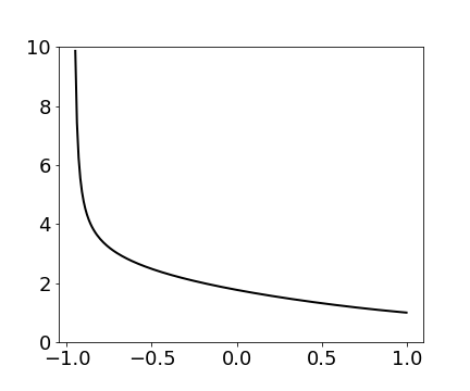
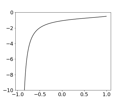
Figure 1: Left: the function $\varphi$ with $\varphi(1)=1$ for $\lambda=\alpha=1/4$, $\mu=1$. Center: the derivative $\varphi^{\prime}$. Right: the solid line is the value function $V^{*}(x,1)$; the dashed line is $V(x)$, $x\in[-1,-B]$ (cf. (17)).

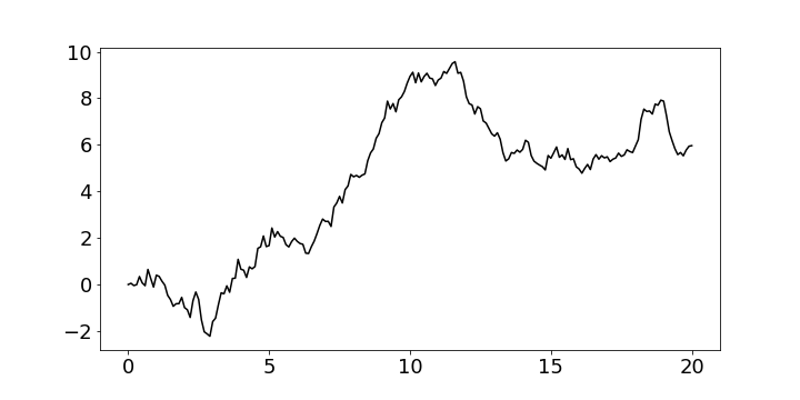
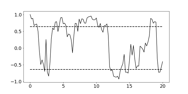
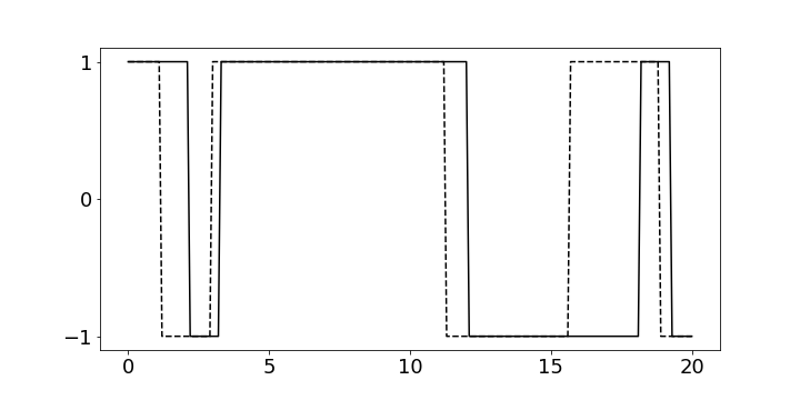
Figure 2: Top: a simulated path of the process $X_{t}$. Center: the posterior mean $M_{t}$ and the thresholds $\pm B$. Bottom: the solid line is the control process $A_{t}$, the dashed line is the unobservable process $\theta_{t}$.

In Figure 1 we show the plot of the approximation of the function $\varphi$ (normalised so that $\varphi(1)=1$) that corresponds to $\lambda=\alpha=1/4$, $\mu=1$, and the plot of its derivative. The plots were obtained by solving the Cauchy problem for (11) with $\varphi(0.9999)=1$ and $\varphi^{\prime}(0.9999)=-0.5$ (cf. the second statement of Proposition 2). We need to step a little to the left from $1$ in setting up the Cauchy problem because (11) is a regular ODE only strictly inside $[-1,1]$ (the coefficient in front of the second derivative vanishes at $\pm 1$).

Finally, being able to obtain good approximations of $\varphi$ we can numerically find the values $(K,B)$ satisfying (15)–(16) (see (26)–(27) below for more detail). For example, for the above values of $\lambda$, $\alpha$, $\mu$ and $c_{1}=1/4$, $c_{2}=0$, we get $B=0.639$ and $K=0.378$ (this value of $K$ corresponds to $\varphi$ normalised by $\varphi(1)=1$; recall that the value of $K$ depends on the chosen version of $\varphi$), which fully determines both the value function $V^{*}(x,1)$ and the optimal strategy.

Figure 2 shows a simulated example of the process $X_{t}$, the posterior mean process $M_{t}$, and the optimal control process $A_{t}$ with the same parameters.

4 Proofs

4.1 Proofs of the auxiliary results

Proof of Proposition 1.

While statements like (a)–(c) belong to common knowledge in the Sturm-Liouville theory, some of their aspects depend on the ODE under consideration. For example, for the ODE $f^{\prime\prime}-f=0$ on $(-1,1)$ (cf. with (11)), the functions $e^{-x}$ and $e^{-x+1}+e^{x-1}$ are non-proportional strictly decreasing strictly positive solutions, that is, the analogue of (b) does not hold true. Therefore, even though the topic is well-studied, we give a short treatment of claims (a)–(c) deducing them from the general theory of one-dimensional diffusions. The analysis below relies on boundary behavior of the process $M$, which is investigated in the appendix.

Consider the diffusion $M$ driven by (8) inside $(-1,1)$ with a starting point $x\in(-1,1)$ under measure $\mathsf{P}_{x}$. Notice that the first- and second-order derivative terms in (9) constitute the generator of $M$, hence the relation between $M$ and ODE (11). As for claim (a) of Proposition 1, the fact that (11) possesses a strictly decreasing (as well as a strictly increasing) strictly positive solution is a well-known fact in the theory of one-dimensional diffusions: e.g., see Proposition 50.3 in Chapter V in [15] or Section II.1.10 in [3]. Moreover, there is a strictly decreasing strictly positive solution $\varphi$ of (11) with the property (analogue of formula (50.5) in Chapter V of [15])

$$\varphi(x)=\varphi(y)\mathsf{E}_{x}\left[e^{-\alpha T_{y}}\right],\quad\text{for all }x>y\text{ in }(-1,1),$$ (22)

where $\alpha>0$ is the one present in (9) and

$$T_{y}=\inf\{t\geq 0:M_{t}=y\}$$

(with the usual convention $\inf\emptyset:=\infty$).

Let $f\colon(-1,1)\to\mathbb{R}$ be a decreasing strictly positive solution to (11). In particular, $f\in C^{2}$. Fix a starting point $x\in(-1,1)$ of $M$ and consider the process $(e^{-\alpha t}f(M_{t}))_{t\geq 0}$, which is well-defined because the boundaries $\pm 1$ are inaccessible for $M$, and is a $\mathsf{P}_{x}$-local martingale by the Itô formula. Then, for any $y\in(-1,x)$, the process $X_{t}:=e^{-\alpha(t\wedge T_{y})}f(M_{t\wedge T_{y}})$, $t\geq 0$, is a bounded $\mathsf{P}_{x}$-martingale. The identity $\mathsf{E}_{x}X_{0}=\mathsf{E}_{x}X_{\infty}$ now yields $f(x)=f(y)\mathsf{E}_{x}\left[e^{-\alpha T_{y}}\right]$. As $x>y$ in $(-1,1)$ are arbitrary, we get that the function $f$ satisfies (22) (in place of $\varphi$). But (22) determines a function up to proportionality (given a value of $f(c)$ for some fixed $c\in(-1,1)$, we uniquely determine $f(x)$ for all $x\in(-1,1)$ via (22)). This implies claim (b).

Finally, for a fixed $x$, let $y\to-1$ in (22). Since the boundary $-1$ is inaccessible for $M$, we have $\mathsf{E}_{x}\left[e^{-\alpha T_{y}}\right]\to 0$ and, therefore, $\varphi(y)\to+\infty$ as $y\to-1$. Let now $x\to 1$ in (22) with a fixed $y$. As $1$ is entrance boundary, we have $\lim_{x\to 1}\mathsf{E}_{x}\left[e^{-\alpha T_{y}}\right]>0$, which means that $\lim_{x\to 1}\varphi(x)>0$. This proves claim (c). ∎

Proof of Proposition 2.

Given arbitrary strictly positive numbers $\lambda$, $\mu$ and $\alpha$, take any decreasing strictly positive solution $\varphi$ to (11).

(a) We have

$$\frac{\mu^{2}}{2}(1-x^{2})^{2}\varphi^{\prime\prime}(x)=2\lambda x\varphi^{\prime}(x)+\alpha\varphi(x),\quad x\in(-1,1),$$ (23)

hence $\varphi^{\prime\prime}>0$ on $(-1,0]$. Let us show that also $\varphi^{\prime\prime}\geq 0$ on $[0,1)$. Indeed, if there was a point $x_{0}\in[0,1)$ such that $\varphi^{\prime\prime}(x_{0})<0$, then $\varphi^{\prime}(x)$ would be locally decreasing at $x_{0}$, from which one would conclude that $2\lambda x\varphi^{\prime}(x)+\alpha\varphi(x)\leq 2\lambda x\varphi^{\prime}(x_{0})+\alpha\varphi(x_{0})$ for any $x\in(x_{0},1)$, which implies that $\varphi^{\prime\prime}(x)\leq\gamma/(1-x^{2})^{2}$ for $x\in(x_{0},1)$ with $\gamma=(1-x_{0}^{2})^{2}\varphi^{\prime\prime}(x_{0})<0$. Integrating twice we would get that $\varphi(x)\to-\infty$ as $x\to 1$, which contradicts the positivity of $\varphi$.

Thus, we have $\varphi^{\prime\prime}(x)\geq 0$ on $(-1,1)$, so $\varphi(x)$ is convex. Moreover, it is actually strictly convex on $(-1,1)$ because otherwise there would be an interval, where $\varphi$ is affine, but there is no affine function locally satisfying (11).

(b) Since $\varphi$ is decreasing and convex on $(-1,1)$, there is a finite limit $\lim\limits_{x\to 1}\varphi^{\prime}(x)$ and

$$\lim_{x\to 1}\varphi^{\prime}(x)\leq 0.$$ (24)

Then it follows from (23) that there is a finite limit $\gamma:=\lim\limits_{x\to 1}(1-x^{2})^{2}\varphi^{\prime\prime}(x)$. Convexity of $\varphi$ yields $\gamma\geq 0$. If we assume that $\gamma>0$, we get $\varphi^{\prime\prime}(x)\geq\frac{1}{2}\gamma/(1-x^{2})^{2}$ for $x\in[y,1)$ with some $y\in(0,1)$. Integrating we obtain $\varphi^{\prime}(x)\to+\infty$ as $x\to 1$, which contradicts (24). Therefore, $\lim\limits_{x\to 1}(1-x^{2})^{2}\varphi^{\prime\prime}(x)=0$, which concludes the proof. ∎

4.2 Proof of the main theorem

1. Consider the case $c_{1}<(2\lambda+\alpha)^{-1}$. It is convenient to define $\beta=(2\lambda+\alpha)^{-1}$ and $\gamma=\frac{c_{1}+{c_{2}}/{2}}{\beta+{c_{2}}/{2}}$. Let us prove that there is a pair $(K,B)$ with $K>0$ and $B\in(\gamma,1)$ such that (15)–(16) hold true, where we set

$$V(x)=\widetilde{V}(x)-K\varphi(x),\quad x\in(-1,1]$$ (25)

(recall that $\widetilde{V}$ is given in (21) and that $\varphi$ satisfies claims (a)–(c) after (11)).

Let us observe that the system (15)–(16) is equivalent to

$$K=h_{1}(B)=h_{2}(B),$$ (26)

where the continuous functions $h_{1}$ and $h_{2}$ are defined on $(0,1)$ by the formulas

$$h_{1}(x)=\frac{(\beta+{c_{2}}/{2})x-c_{1}-{c_{2}}/{2}}{\varphi(-x)-\varphi(x)},\quad h_{2}(x)=\frac{\beta+c_{2}/2}{-\varphi^{\prime}(-x)-\varphi^{\prime}(x)}.$$ (27)

Notice that not only $\varphi$ is strictly decreasing on $(-1,1)$, but also $\varphi^{\prime}<0$ everywhere on $(-1,1)$, so that we have strictly positive quantities in the denominators. Indeed, if $\varphi^{\prime}(x_{0})=0$ at some point $x_{0}\in(-1,1)$, then, by (11), $\varphi^{\prime\prime}(x_{0})>0$, hence $\varphi^{\prime}$ would be strictly positive in a right neighbourhood of $x_{0}$. This would contradict the fact that $\varphi$ is decreasing.

Since we are considering the case $c_{1}<\beta$, the function $h_{1}$ is negative on $(0,\gamma)$ and positive on $(\gamma,1)$, while the function $h_{2}$ is positive everywhere on $(0,1)$. Therefore, in order to prove that the system (15)–(16) has a solution $(K,B)\in(0,\infty)\times(\gamma,1)$, it is sufficient to show that $h_{1}(x)/h_{2}(x)\geq 1$ for some $x\in(\gamma,1)$. Let $\varepsilon>0$ be such that $\gamma+\varepsilon<1$. Then for $x\in[\gamma+\varepsilon,1)$ we have

$$\frac{h_{1}(x)}{h_{2}(x)}=(x-\gamma)\,\frac{-\varphi^{\prime}(-x)-\varphi^{\prime}(x)}{\varphi(-x)-\varphi(x)}\geq\varepsilon\frac{-\varphi^{\prime}(-x)}{\varphi(-x)},$$

hence it will be enough to establish that $\limsup_{x\to 1}(-\varphi^{\prime}(-x)/\varphi(-x))=+\infty$, or, equivalently, with $f(x):=\varphi^{\prime}(x)/\varphi(x)$, that it holds

$$\liminf_{x\to-1}f(x)=-\infty.$$ (28)

Dividing the homogeneous equation $L\varphi=0$ by the function $\varphi$, we get

$$\frac{\mu^{2}}{2}(1-x^{2})^{2}(f^{\prime}(x)+f^{2}(x))-2\lambda xf(x)=\alpha,$$

which implies

$$f^{\prime}(x)+f^{2}(x)=\frac{2(\alpha+2\lambda xf(x))}{\mu^{2}(1-x^{2})^{2}}.$$

Observe that $f(x)\leq 0$, hence, if $x\leq 0$, then the right-hand side is strictly positive and tends to $+\infty$ as $x\to-1$. If we suppose that $f$ is bounded in a right neighbourhood of $-1$, then, for some $\varepsilon>0$, we have $f^{\prime}(x)\geq\varepsilon/(1-x^{2})^{2}$ in a right neighbourhood of $-1$, and integrating we obtain a contradiction with the boundedness of $f$, which proves (28). Thus, the system (15)–(16) has a solution $(K,B)\in(0,\infty)\times(\gamma,1)$. Its uniqueness will be proved later.

2. Let us take any solution $(K,B)\in(0,\infty)\times(\gamma,1)$ of the system (15)–(16) and, with the function $V(x)$ given by (25), define the “candidate” value function $V(x,a)$, $x\in[-1,1]$, $a\in\{-1,1\}$, as the right-hand side of (17):

$$V(x,1) =\begin{cases}V(x),&x\in[-B,1],\\ V(-x)+c_{1}+\dfrac{c_{2}}{2}(1+x),&x\in[-1,-B),\end{cases}$$ (29)

$$V(x,-1) =V(-x,1),\quad x\in[-1,1].$$ (30)

We are going to prove that $V(x,a)$ defined in this way coincides with the value function $V^{*}(x,a)$ defined in (4), where $J(x,A)$ admits representation (20).

Before we are able to do this, we need to establish the following auxiliary facts:

1. $V^{\prime}(x,a)$ is bounded for $x\in[-1,1]$, where by $V^{\prime}(x,a)$ we will denote the derivative with respect to the first argument;

2. $|\Delta V(x,a)|\leq c_{1}+\frac{c_{2}}{2}(1+x)$ for $x\in[-1,1]$, where $\Delta V(x,a):=V(x,a)-V(x,-a)$;

3. $V(x,a)\in C^{1}$ in $x\in[-1,1]$, $V(x,a)\in C^{2}$ in $x$ except at points $x=\pm B$, and $LV(x,a)\geq-\frac{1}{2}(1-ax)$ for $x\in[-1,1]\setminus\{-B,B\}$.

Due to the symmetry, it is enough to consider only $V(x,1)$. As for (F1), by (29) it is enough to establish boundedness of $V^{\prime}(x,1)$ in a left neighbourhood of $1$. The latter follows from (25) and the fact that $\varphi$ is decreasing and convex (recall Proposition 2).

Let us prove that (F2). Denote for convenience

$$g(x):=\Delta V(x,1)\;(\equiv V(x,1)-V(-x,1)).$$

According to the definition of $V(x,a)$, we immediately have $|g(x)|=c_{1}+\frac{c_{2}}{2}(1+x)$ for $|x|\geq B$. In particular, $g(-B)=c_{1}+\frac{c_{2}}{2}(1-B)$, $g(B)=-c_{1}-\frac{c_{2}}{2}(1+B)$, so it is sufficient to show that $g$ is decreasing on $[-B,B]$.

Considering the second derivative of $g$ in $(-B,B)$, $g^{\prime\prime}(x)=-K(\varphi^{\prime\prime}(x)-\varphi^{\prime\prime}(-x))$, and recalling that (as follows from (11))

$$\varphi^{\prime\prime}(x)=\frac{2}{\mu^{2}}\,\frac{2\lambda x\varphi^{\prime}(x)+\alpha\varphi(x)}{(1-x^{2})^{2}},$$

hence, for $x<0$,

$$\varphi^{\prime\prime}(x)\geq\frac{2}{\mu^{2}}\,\frac{\alpha\varphi(x)}{(1-x^{2})^{2}}>\frac{2}{\mu^{2}}\,\frac{\alpha\varphi(-x)}{(1-x^{2})^{2}}\geq\varphi^{\prime\prime}(-x),$$

we get $g^{\prime\prime}(x)<0$ and $g^{\prime}(x)$ is strictly decreasing for $x\in[-B,0)$. In a similar way, $g^{\prime}(x)$ is strictly increasing for $x\in(0,B]$. These two facts combined with that $g^{\prime}(-B)=g^{\prime}(B)=0$ (according to (16)), mean that $g^{\prime}(x)<0$ for $x\in(-B,B)$, so $g$ is decreasing on $[-B,B]$. Thus, fact (F2) is proved.

Finally, the differentiability properties of $V(x,1)$ follow from its definition together with (16), and, since $\widetilde{V}(x)$ solves the inhomogeneous ODE, while $\varphi(x)$ solves the homogeneous ODE, we have

$$LV(x,1)=-\frac{1}{2}(1-x)\text{ for }x\in(-B,1),$$

$$LV(x,1)=-\frac{1}{2}(1+x)-\alpha c_{1}-\frac{c_{2}}{2}(2\lambda x+1+x)\text{ for }x\in(-1,-B).$$

Using that $c_{1}<\beta$ and $B>\gamma$ one can check that $LV(x,1)>-\frac{1}{2}(1-x)$ for $x\in(-1,-B)$, which completes the proof of (F3).

3. Now we continue with proving that $V(x,a)$ defined in (29)–(30) coincides with the value function $V^{*}(x,a)$. Consider a control process $A_{t}$ starting in $A_{0-}=a$ and let $(\tau_{n})_{n=0}^{\infty}$ be the corresponding sequence of stopping times (see (5)–(6)). By the Itô formula we have for any $n\geq 1$

$$e^{-\alpha\tau_{n}}V(M_{\tau_{n}},A_{\tau_{n}})=V(M_{0},a)+\sum_{1\leq k\leq n}\biggl{[}\int_{\tau_{k-1}}^{\tau_{k}}e^{-\alpha s}LV(M_{s},A_{s})ds\\ +\mu\int_{\tau_{k-1}}^{\tau_{k}}e^{-\alpha s}(1-M_{s}^{2})V^{\prime}(M_{s},A_{s})\,d\overline{W}_{s}+e^{-\alpha\tau_{k}}\Delta V(M_{\tau_{k}},A_{\tau_{k}})\biggr{]}.$$

Taking the expectation under $\mathsf{P}_{x}$ of the both sides and letting $n\to\infty$, so that $\tau_{n}\to\infty$, we obtain

$$V(x,a)=-\mathsf{E}_{x}\sum_{k\geq 1}\biggl{[}\int_{\tau_{k-1}}^{\tau_{k}}e^{-\alpha s}LV(M_{s},A_{s})ds+e^{-\alpha\tau_{k}}\Delta V(M_{\tau_{k}},A_{\tau_{k}})\biggr{]},$$

where it was used that the stochastic integral is a uniformly integrable martingale (since $V^{\prime}(x,a)$ is bounded as proved in (F1) above), so its expectation is zero.

From (F2)–(F3) proved above, we get

$$V(x,a)\leq\mathsf{E}_{x}\biggl{[}\frac{1}{2}\int_{0}^{\infty}e^{-\alpha s}(1-A_{s}M_{s})\,ds\\ +\sum_{s\geq 0}e^{-\alpha s}I(\Delta A_{s}\neq 0)\Bigl{(}c_{1}+\frac{c_{2}}{2}(1-A_{t}M_{t})\Bigr{)}\biggr{]}.$$ (31)

Taking the infimum over all $A\in\mathcal{A}_{a}$ we see that

$$V(x,a)\leq V^{*}(x,a),\quad x\in[-1,1].$$

Furthermore, if we define the control process $A^{*}$ as in (18) in the case $a=1$, respectively as in (19) in the case $a=-1$, then we have $LV(M_{s},A^{*}_{s})=-\frac{1}{2}(1-A^{*}_{s}M_{s})$ for all $s\in(0,\infty)\setminus\{\tau_{k}:k\geq 1\}$ and $\Delta V(M_{\tau_{k}},A^{*}_{\tau_{k}})=-(c_{1}+\frac{c_{2}}{2}(1-A_{s}^{*}M_{s}))$ for all $k\geq 1$, so that (31) turns into equality, i.e., we get

$$V(x,a)=\mathsf{E}_{x}\biggl{[}\frac{1}{2}\int_{0}^{\infty}e^{-\alpha s}(1-A^{*}_{s}M_{s})\,ds\\ +\sum_{s\geq 0}e^{-\alpha s}I(\Delta A^{*}_{s}\neq 0)\Bigl{(}c_{1}+\frac{c_{2}}{2}(1-A_{S}^{*}M_{s})\Bigr{)}\biggr{]}.$$

Consequently, $V^{*}(x,a)=V(x,a)$.

4. The final step in considering the case $c_{1}<\beta$ is to prove uniqueness of the pair $(K,B)\in(0,\infty)\times(\gamma,1)$ that satisfies (15)–(16), where the function $V(x)$, $x\in[-1,1]$, is given by (25). Suppose there are two such pairs $(K_{1},B_{1})$ and $(K_{2},B_{2})$ and denote by $V_{1}(x,a)$, $V_{2}(x,a)$ the respective functions defined by (29)–(30). Without loss of generality assume $B_{1}\leq B_{2}$.

According to the reasoning in part 4.2 of the proof, both $V_{1}$ and $V_{2}$ coincide with the value function $V^{*}$. In particular, $V_{1}(x,1)=V_{2}(x,1)$ for $x\in[-B_{1},1]$, which readily implies $K_{1}=K_{2}$.

Suppose $B_{1}<B_{2}$. Denote $V(x)=\widetilde{V}(x)-K\varphi(x)$ with $K=K_{1}\;(=K_{2})$. It follows from (29) and the equality $V_{1}(x,1)=V_{2}(x,1)$ that $V(x)=V(-x)+c_{1}+\frac{c_{2}}{2}(1+x)$ for $x\in[-B_{2},-B_{1}]$, i.e.,

$$g(x):=V(x)-V(-x)\equiv c_{1}+\frac{c_{2}}{2}(1+x)\quad\text{on }[-B_{2},-B_{1}].$$ (32)

However, by the treatment of (F2) in part 4.2 of this proof, $g^{\prime\prime}(x)<0$ for $x\in(-B_{2},B_{2})$, which contradicts (32). Therefore, $B_{1}=B_{2}$.

5. Finally, let us consider the case $c_{1}\geq\beta$. The proof of part (i) of Theorem 1 is completed by now, and we are going to use it. To this end, we extend the previous notation to stress the dependence of the involved functions and constants on $c_{1}$. In particular, for all $c_{1}\geq 0$, $V^{*}(x,1)$ will now be denoted by $V^{*}_{c_{1}}(x,1)$; for $c_{1}\in[0,\beta)$, the constants $K$ and $B$ determined by (14)–(16) will be denoted by $K_{c_{1}}$ and $B_{c_{1}}$ (we consider the same version of $\varphi$ for different values of $c_{1}$, e.g., the version obtained by the normalisation $\varphi(1)=1$). Also, for $c_{1}\in(0,\beta)$, we set

$$V_{c_{1}}(x)=\widetilde{V}(x)-K_{c_{1}}\,\varphi(x),\quad x\in(-1,1]$$ (33)

As $B_{c_{1}}\in(\gamma_{c_{1}},1)$ for $c_{1}\in(0,\beta)$, we have $\lim_{c_{1}\to\beta}B_{c_{1}}=1$. Furthermore, it follows from (26)–(27) that $\lim_{c_{1}\to\beta}K_{c_{1}}=0$. Together with (17), this yields

$$\lim_{c_{1}\to\beta}V^{*}_{c_{1}}(x,1)=\widetilde{V}(x),\quad x\in[-1,1].$$

More precisely, for $x\in(-1,1]$, use (17), $B_{c_{1}}\to 1$, (33), and $K_{c_{1}}\to 0$, while, for $x=-1$, use additionally that $\widetilde{V}(-1)=\widetilde{V}(1)+\beta$. Since, clearly, $V^{*}_{c_{1}}(x,1)$ is increasing in ${c_{1}}$ (for any $x\in[-1,1]$), we obtain

$$V^{*}_{c_{1}}(x,1)\geq\widetilde{V}(x),\;\;x\in[-1,1],\quad\text{for all }c_{1}\geq\beta.$$

It remains to recall that, for any $c_{1}\geq\beta$, the strategy $A^{*}\in\mathcal{A}_{1}$ with $A^{*}\equiv 1$ produces the cost $\widetilde{V}(x)$. This concludes the proof.

Appendix: Boundary behaviour of the process $M$

In this appendix we show that the posterior mean process $M$ is a regular diffusion in $(-1,1)$ with $\pm 1$ being inaccessible entrance boundaries. Such a characterization of the boundaries conceptually means that if a solution to (8) is started at a point $x\in(-1,1)$, then it never reaches the boundaries $\pm 1$. If a solution is started at $x=\pm 1$, then it immediately enters the interval $(-1,1)$ and never leaves it.

So, let us consider $M$ driven by (8) with a starting point $x\in(-1,1)$. The regularity follows from that $(1+|b(x)|)\sigma^{-2}(x)$ is a locally integrable function in $(-1,1)$, where $b(x):=-2\lambda x$ is the drift coefficient and $\sigma(x):=\mu(1-x^{2})$ is the diffusion coefficient (see Section 5.5.C and, in particular, conditions (ND)’ and (LI)’ in [9]).

The scale function of $M$ is given by the formula

$$p(x)=\int_{0}^{x}\exp\left\{\frac{2\lambda}{\mu^{2}}\frac{1}{1-y^{2}}\right\}dy,\quad x\in(-1,1).$$

Since $p(\pm 1)=\pm\infty$, the boundaries $\pm 1$ are inaccessible (see Proposition 5.5.22 in [9]).

The speed measure of $M$ is

$$m(dx)=\frac{2\,dx}{p^{\prime}(x)\mu^{2}(1-x^{2})^{2}}\,dx\quad\text{on }(-1,1).$$

Let us show that

$$\int_{(0,1)}p(y)\,m(dy)<\infty,$$ (34)

which implies that $1$ is an entrance boundary for $M$ (see Section II.1.6 in [3]), and, by symmetry, $-1$ is an entrance boundary as well.

In order to prove (34) it is enough to establish that there is a finite limit

$$\gamma:=\lim_{x\to 1}\frac{p(x)}{p^{\prime}(x)(1-x^{2})^{2}}.$$

We have

$$p^{\prime}(x)=\exp\left\{\frac{2\lambda}{\mu^{2}}\frac{1}{1-x^{2}}\right\},\qquad p^{\prime\prime}(x)=p^{\prime}(x)\frac{4\lambda}{\mu^{2}}\frac{x}{(1-x^{2})^{2}}.$$

Since the limit $\gamma$ is of the type $\frac{\infty}{\infty}$, by l’Hôpital’s rule, we find

$$\gamma=\lim_{x\to 1}\frac{p^{\prime}(x)}{p^{\prime\prime}(x)(1-x^{2})^{2}-2p^{\prime}(x)(1-x^{2})x}=\frac{\mu^{2}}{4\lambda}.$$

References

- Bayraktar and Egami [2010] E. Bayraktar and M. Egami. On the one-dimensional optimal switching problem. Mathematics of Operations Research, 35(1):140–159, 2010.