Distributed Adaptive Coverage Control of Differential Drive Robotic Sensors

Abstract

This paper is concerned with the deployment of multiple mobile robots in order to autonomously cover a region $\mathcal{Q}$. The region to be covered is described using a density function which may not be apriori known. In this paper, we pose the coverage problem as an optimization problem over some space of functions on $\mathcal{Q}$. In particular, we look at $\mathcal{L}^{2}$-distance based coverage algorithm and derive adaptive control laws for the same. We also propose a modified adaptive control law incorporating consensus for better parameter convergence. We implement the algorithms on real differential drive robots with both simulated density function as well as density function implemented using light sources. We also compare the $\mathcal{L}^{2}$-distance based method with the locational optimization method using experiments.

1 Introduction

Cooperative control problems involving multi-agent systems have been widely studied in the literature. We consider multiple autonomous agents that work together to achieve an objective. Objectives include rendezvous where the agents try to converge to a common state, formation control where the agents try to maintain a given spatial formation and coverage control where the agents are deployed to cover a given region of interest. See Jadbabaie and Lin (2003); Murray (2007); Olfati-Saber et al. (2007); Tanner et al. (2007); Cortes et al. (2004); Bullo et al. (2009); Song et al. (2011, 2013). These cooperative control algorithms find applications in surveillance, patrolling, environmental monitoring and sensing etc.

The agents communicate with each other using some communication topology which is described in terms of a graph where the nodes correspond to the agents and two nodes are connected if the two corresponding agents can communicate with each other. In most cases, communication graphs correspond to proximity graphs meaning that two agents communicate if they are close to each other. This also motivates the use of decentralized or distributed control strategies for efficient solution of multiagent problems where the control laws of individual agents are determined by the information exchange with their neighbouring agents See for example Murray (2007); Olfati-Saber et al. (2007); Bullo et al. (2009).

In this paper, we consider the problem of optimally covering a given region using multiple agents to sense a phenomenon/event of interest. The event of interest is described by a density function over the region. The density function can be thought of as giving the distribution of the intensity of the phenomenon to be sensed. For example, in case of mobile agents deployed to sense nuclear radiation over a region, the density function could be the intensity of radiation over the region. In this case, we would like the mobile agents which are deployed starting at some initial position to converge to some optimal configuration for sensing purpose.

The coverage problem in the locational optimization framework was investigated in in Cortes et al. (2004), where $n$ agents are deployed to cover a convex region $\mathcal{Q}\subset\mathbb{R}^{q}$. The problem was solved for agents with single integrator dynamics and known density function. In Schwager et al. (Apr. 10-14, 2007) and Schwager et al. (2009), the authors extend the algorithm of Cortes et al. (2004) using adaptive control for the case where the density function is not fully known. The density function is assumed to be linearly parameterized in terms of a vector of unknown constant parameters. They also propose a consensus term in the adaptation law which improves parameter convergence. In Cortes and Bullo (2005), the authors discuss spatial optimization problems closely related to coverage problems using gradient descent methods. In Hexsel et al. (2011); Guruprasad and Ghose (2013); Bopardikar et al. (2018), the authors talk about different versions of the coverage problem based on locational optimization by using different assumptions on the agent sensing capabilities. The adaptive coverage algorithms have been extended to nonholonomic robots in Luna et al. (2013); Abdul Razak et al. (2018). In many problems, it would be also be beneficial to estimate the parameters of the density function correctly along with the coverage task. In this case, the issue of parameter estimation becomes important. The parameters converge to true values provided an integral condition over the trajectories of the agents are satisfied which may not always be achieved. There are not many works in the literature which focus on the issue of parameter estimation in the context of coverage control.

In this work, we pose the coverage problem in a general framework. The agents located at different positions in the domain can be thought of as defining an agent density function. The coverage problem can then be posed as an optimization problem which seeks to minimize the distance between the original density function and the agent density function for some appropriately defined distance. This approach is more general in the sense that the locational optimization problem can be viewed as a special case of this formulation. We in addition look at the $\mathcal{L}^{2}$-metric for achieving coverage and derive adaptive control laws for differential drive robots. We also present a slightly modified adaptive control law using consensus over directed sub-graphs of the delaunay graph for improving parameter convergence. The algorithms described are tested on actual differential drive robots and a comparison is given between the $\mathcal{L}^{2}$-distance based approach and the locational optimization approach in Cortes et al. (2004); Abdul Razak et al. (2018). We are particularly interested in studying how the two approaches handle the problem of parameter estimation. A part of the current work has been presented at Razak et al. (2018).

In section 2, we formulate and discuss the coverage problem. In section 3, we discuss a new objective function based on $\mathcal{L}^{2}$-distance for achieving coverage. In section 4 we derive control and adaptation laws for differential drive robots to converge to near optimal configuration. We also discuss some improvements to the parameter adaptation law which gives better parameter convergence. In section 5 we discuss experimental results on differential drive robots and also give a comparison of the $\mathcal{L}^{2}$ method with the locational optimization. Finally we conclude the paper with section 6.

2 Problem Formulation

We consider a bounded convex region $\mathcal{Q}\subset\mathbb{R}^{n}$ where $N$ agents are deployed so as to spread and distribute themselves in an optimal manner with respect to a density function $\phi:\mathcal{Q}\to\mathbb{R}_{+}$ where $\mathbb{R}_{+}$ is the set of positive real numbers. The density function $\phi(.)$ represents the event of interest with respect to which coverage is to be obtained (also called $\phi(.)$ the target density). Intuitively we want more robots to be concentrated over regions having higher values of the density function. The positions of the agents are denoted by $p_{i}$ for $i=1,2,\dots,N$ and the set of all agent positions is denoted by $P$. For a given configuration of agents $P=\{p_{i}\}_{i=1}^{N}$, we define the voronoi partition of $\mathcal{Q}$ as the set $\{\mathcal{V}_{i}\}_{i=1}^{N}$ where

$$\centering\mathcal{V}_{i}=\{q\in\mathcal{Q}\,\mid\,\|q-p_{i}\|\leq\|q-p_{j}\|,\,\,\forall j\neq i\}.\@add@centering$$ (1)

The voronoi cell $\mathcal{V}_{i}$ is the set of all points closest to agent $i$ compared to all the other agents. In Cortes et al. (2004), the optimal coverage configuration is described as the optimum of the locational optimization cost

$$\centering\mathcal{H}(P)=\sum_{i=1}^{N}\int\limits_{\mathcal{V}_{i}}\|p_{i}-q\|^{2}\phi(q)dq\@add@centering$$ (2)

In this paper, we formulate the coverage problem in a more general framework, as an optimization problem over a space of functions over $\mathcal{Q}$.

2.1 Distance Function based Approach

Each agent is assumed to have a sensing capability which decreases with the distance from the agent location. We quantify this sensing capability of each agent as the sensing function denoted by $f_{i}(p_{i},q)$. The sensing function describes the capability of the agent at position $p_{i}$ to sense event at point $q$. In this work we assume isotropic sensors whose sensing is independent of direction. We can thus represent the sensing function as $f_{i}(\|p_{i}-q\|)$. We require $f_{i}:\mathbb{R}_{+}\to\mathbb{R}_{+}$ to be an appropriate decreasing function of its argument. An illustration for the one-dimensional case is shown in figure 1.

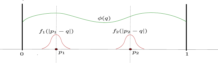
Figure 1: Two agents covering the interval $\mathcal{Q}=[0,1]$

Given $N$ agents each with its sensing functions, we define an aggregate agent density function defined by

$$f_{P}(q):=\alpha(f_{1}(\|p_{1}-q\|),f_{2}(\|p_{2}-q\|),\dots,f_{N}(\|p_{N}-q\|))$$

where $\alpha:\mathbb{R}_{+}^{N}\to\mathbb{R}_{+}$ is an aggregation function which is to be chosen appropriately. The aggregate agent density gives a measure of the quality of sensing of the region $\mathcal{Q}$ using all the $N$ agents. The general coverage problem can then be posed as the following optimization problem:

$$\min_{P=\{p_{1},p_{2},\dots,p_{N}\}}d(\phi,f_{P})$$ (3)

where $d(.,.)$ is an appropriate measure of divergence or distance between $\phi$ and $f_{P}$. The agents should move to a configuration such that the distance between the target density $\phi$ and the aggregate agent density $f_{P}$ is minimized. The choice of $d(.,.)$ will generally be determined by the class of functions we work with which depends on the nature of the coverage density function $\phi(.)$ as well as the nature of sensors in the mobile agents employed. The optimal locations of the agents is then given by

$$P^{*}=\{p_{1}^{*},p_{2}^{*},\dots,p_{N}^{*}\}=\mbox{arg}\min_{P}d(\phi,f_{P})$$ (4)

2.2 Choice of the agent sensing functions and aggregate density

The agent sensing functions $f_{i}(\|p_{i}-q\|)$ as mentioned above is required to be a non-increasing function of its argument, and depends on the nature of sensors. Some examples which we can be used are given below:

1. Gaussian function

   $$f_{i}(x)=A_{i}\exp\left(-\frac{x^{2}}{\sigma_{i}^{2}}\right)$$ (5)

   for some constants $A_{i}>0$, $\sigma_{i}>0$.

2. Constant sensing function

   $$f_{i}(x)=\mathcal{\chi}_{\{x\leq r_{i}\}}$$ (6)

   where $\mathcal{\chi}_{S}$ is the characteristic function of the set $S$ and $r_{i}>0$ is some constant.

3. Quartic function

   $$f_{i}(x)=\left\{\begin{array}[]{ll}\frac{M}{r_{i}^{4}}\left(x^{2}-r_{i}^{2}\right)^{2}&\mbox{ if }x<r_{i}\\ 0&\mbox{ if }x\geq r_{i}\end{array}\right.$$ (7)

   for some constants $M>0,r_{i}>0$.

4. Bump function

   $$f_{i}(x)=\left\{\begin{array}[]{ll}A_{i}\exp\left\{-\frac{1}{1-\left(\frac{x}{r_{i}}\right)^{2}}\right\}&\mbox{ if }x<r_{i}\\ 0&\mbox{ if }x\geq r_{i}\end{array}\right.$$ (8)

   for some constant $A_{i}>0$, $r_{i}>0$.

The constant sensing function, the bump function and the quartic function (unlike the Gaussian function) allow us to model sensors with a finite sensing range since they take zero value outside a finite region of radius $r_{i}$ around the agent position. Accordingly, we consider these functions as examples of limited range sensing functions, and the Gaussian function as an example of a full range sensing function. The choice of aggregate agent density $f_{P}(\cdot)$ could be made in different ways. We give here two natural choices:

1. Average/sum function

   $$f_{P}(q)=\gamma\sum_{i=1}^{N}f_{i}(\|p_{i}-q\|)$$ (9)

2. Max function

   $$f_{P}(q)=\gamma\max_{i}f_{i}(\|p_{i}-q\|)$$ (10)

where $\gamma$ is some positive constant. The max function defines the aggregate density at a point as the value of the agent sensing function with the maximum value at the point. If the agents are identical, then the aggregate density at a point in this case is the agent density corresponding to the agent that is closest to the point. We will see that this naturally leads to a partition of the region $\mathcal{Q}$ and allows using distributed control schemes.

2.3 Locational Optimization

Now, we consider the locational optimization problem defined by the cost function [see Cortes et al. (2004)]

$$\mathcal{H}(p_{1},\dots,p_{N}) =\int_{Q}\min_{i}\|p_{i}-q\|^{2}\phi(q)dq$$ (11)

$$=\sum_{i=1}^{N}\int_{\mathcal{V}_{i}}\|p_{i}-q\|^{2}\phi(q)dq$$ (12)

where the domain $\mathcal{Q}$ is assumed to be compact and convex, $p_{i}$ are the locations of the agents and {$\mathcal{V}_{i}$} is the voronoi partition of $\mathcal{Q}$ corresponding to $\{p_{i}\}$. The minimizer of the function $\mathcal{H}$ correspond to the centroidal voronoi configuration. These are the points $p_{i}^{*}$ such that $p_{i}^{*}=C_{\mathcal{V}_{i}}$ where $C_{\mathcal{V}_{i}}=(\int_{\mathcal{V}_{i}}q\phi(q)dq)/(\int_{\mathcal{V}_{i}}\phi(q)dq)$.

We wish to pose the locational optimization problem in the general framework discussed above (equation (3)). In order to do that we consider the relative entropy or Kullback-Leibler divergence of two integrable functions $f:\mathcal{Q}\to\mathbb{R}_{+}$ and $g:\mathcal{Q}\to\mathbb{R}_{+}$ where $g(q)>0$, defined as

$$d_{KL}(f,g)=\int_{Q}f(q)\log(\frac{f(q)}{g(q)})dq$$ (13)

$d_{KL}$ is not a metric (since it is not symmetric) but it is a measure of divergence (distance) of $g$ with respect to $f$ and $d_{KL}(f,f)=0$ [see Kullback and Leibler (1951); Press (2007)]. If we interpret the density function $\phi$ as defining the probability density of events occurring in the domain $\mathcal{Q}$, and agent sensing functions as defining the probability of detecting an event, then minimizing $d_{KL}(\phi,f_{P})$ would mean that we are choosing those agent positions which results in maximum likelihood of detection of these events.

Proposition 1

Assume that

• The target density $\phi(.)$ is integrable.

• The sensing functions of the agents are gaussian (equation (5)) with $A_{i}=1$ and $\sigma_{i}=1$.

• The aggregate density function of the agents is given by the max function (10) with $\gamma=1$.

Under the above assumptions,

$$\underset{P}{\arg\min}\,\,\,d_{KL}(\phi,f_{P})=\underset{P}{\arg\min}\,\,\,\mathcal{H}(P)$$

i.e. minimizing $d_{KL}(\phi,f_{P})$ is equivalent to minimizing $\mathcal{H}(P)$.

Proof

For each agent $i$

$$f_{i}(\|p_{i}-q\|)=\exp(-\|p_{i}-q\|^{2})$$

and the aggregate density is given by

$$f_{P}(q)=\max_{i}\,\exp(-\|p_{i}-q\|^{2})$$

Then,

$$d_{KL}(\phi,f_{P}) =\int_{Q}\phi(q)\log\frac{\phi(q)}{f_{P}(q)}dq$$

$$=\int_{Q}\phi(q)\log\phi(q)dq-\int_{Q}\phi(q)\log f_{P}(q)dq$$

Since the first term is independent of $P$, we have

$$\min_{P}d_{KL}(\phi,f_{P}) =\min_{P}-\int_{Q}\phi(q)\log f_{P}(q)dq$$

$$=\min_{P}-\int_{Q}\phi(q)\log\max_{i}f_{i}(\|p_{i}-q\|)dq$$

$$=\min_{P}-\int_{Q}\phi(q)\max_{i}\log f_{i}(\|p_{i}-q\|)dq$$

$$=\min_{P}\int_{Q}\phi(q)\min_{i}\|p_{i}-q\|^{2}dq$$

$$=\min_{P}\mathcal{H}(P)$$

It can be shown [Cortes et al. (2004)] that for agents with single integrator dynamics $\dot{p}_{i}=u_{i}$, the gradient control law given by

$$u_{i}=-\frac{\partial\mathcal{H}}{\partial p_{i}}=-kM_{\mathcal{V}_{i}}(p_{i}-C_{\mathcal{V}_{i}})$$

allows the agents to coverge to the centroidal voronoi configuration.

3 $\mathcal{L}^{2}$-distance based coverage

We assume that the target density $\phi$ belong to $\mathcal{L}^{2}(\mathcal{Q})$. We further assume that $\phi$ is lower bounded, i.e., $\phi(q)\geq\beta$ for some constant $\beta>0$. Assuming that the aggregate density of the agents also belong to $\mathcal{L}^{2}(\mathcal{Q})$, we can define the following cost function

$$d_{2}(\phi,f_{P})=\int_{Q}|\phi(q)-f_{P}(q)|^{2}dq$$ (14)

We now investigate the multiagent coverage problem using the above cost function. Any minima of the cost function $d_{2}(.,.)$ with respect to $P$ satisifies the condition $\frac{\partial d_{2}}{\partial p_{i}}=0$ for every $i$. Let $\mathcal{Q}\subset\mathbb{R}^{n}$ be a convex and bounded region with $N$ agents and let

$$f_{P}(q) =\gamma\max_{i}f(\|p_{i}-q\|)$$

where the agent sensing function $f(.)$ is assumed to be the same for all the agents. Then

$$d_{2}(\phi,f_{P}) =\int_{\mathcal{Q}}\left|\phi(q)-f_{P}(q)\right|^{2}dq$$ (15)

$$=\int_{\mathcal{Q}}\left|\phi(q)-\gamma\left[\max_{i}f(\|p_{i}-q\|)\right]\right|^{2}dq$$

Since $f(.)$ is a decreasing function of its argument, we can write the above as

$$d_{2}(\phi,f_{P})=\sum_{i=1}^{N}\int_{\mathcal{V}_{i}}\left|\phi(q)-\gamma.f(\|p_{i}-q\|)\right|^{2}dq$$ (16)

where $\{\mathcal{V}_{i}\}_{i=1}^{N}$ is the voronoi partition defined by equation (1).

Lemma 1

The gradient of the $\mathcal{L}^{2}$ cost function (16) with respect to $p_{i}$ is given by

$$\frac{\partial d_{2}}{\partial p_{i}}=\int_{\mathcal{V}_{i}}\frac{\partial}{\partial p_{i}}\left|\phi(q)-\gamma.f(\|p_{i}-q\|)\right|^{2}dq$$ (17)

Proof

Computing the gradient with respect to $p_{i}$,

$$\frac{\partial d_{2}}{\partial p_{i}} =\frac{\partial}{\partial p_{i}}\int_{\mathcal{V}_{i}}\left|\phi(q)-\gamma.f(\|p_{i}-q\|)\right|^{2}dq$$ (18)

$$\,\,+\sum_{j\in\mathcal{N}_{i}}\frac{\partial}{\partial p_{i}}\int_{\mathcal{V}_{j}}\left|\phi(q)-\gamma.f(\|p_{j}-q\|)\right|^{2}dq$$

It should be noted that in the expression above the regions of integration $\mathcal{V}_{i}$ and $\mathcal{V}_{j}$ are themselves functions of $p_{i}$. Thus we have [see Cortes et al. (May, 2002); Flanders (1973)]

$$\frac{\partial d_{2}}{\partial p_{i}} =\int_{\mathcal{V}_{i}}\frac{\partial}{\partial p_{i}}\left|\phi(q)-\gamma.f(\|p_{i}-q\|)\right|^{2}dq$$ (19)

$$\,\,+\int_{\partial\mathcal{V}_{i}}\left|\phi(q)-\gamma.f(\|p_{i}-q\|)\right|^{2}n_{iq}^{\scriptscriptstyle\top}\frac{\partial q}{\partial p_{i}}dq$$

$$\,\,+\sum_{j\in\mathcal{N}_{i}}\int_{c_{ij}}\left|\phi(q)-\gamma.f(\|p_{j}-q\|)\right|^{2}n_{jq}^{\scriptscriptstyle\top}\frac{\partial q}{\partial p_{i}}dq$$

where $\partial\mathcal{V}_{i}$ is the boundary of the voronoi region $\mathcal{V}_{i}$ , $\mathcal{N}_{i}$ is the set of voronoi neighbours of agent $i$, $n_{iq}$ is the unit normal at point $q$ pointing outward from the region $\mathcal{V}_{i}$ and $c_{ij}$ is the boundary segment of voronoi region $\mathcal{V}_{i}$ that is shared with the voronoi region of agent $j$ ($\mathcal{V}_{j}$) [see also Cortes et al. (May, 2002)]. The boundary $\partial\mathcal{V}_{i}$ consists of segments $c_{ij}$ and possibly parts of $\partial\mathcal{Q}$ (the boundary of $\mathcal{Q}$). The integrand of the second term is zero over $\partial\mathcal{Q}$. Thus the second and third terms in the above expression cancel each other (since the outward normals $n_{iq}$ and $n_{jq}$ in the two terms point opposite to each other) and the proof is complete.

As a simple example, consider $\mathcal{Q}=[0,1]$ with one agent with $f(|p-q|)=\exp\{-|p-q|^{2}\}=:f_{P}(q)$. Assume the density function is given by $\phi(q)=\exp\{-|c-q|^{2}\}$ for some $c\in(0,1)$. Minimizing the $\mathcal{L}^{2}$ norm implies $\frac{\partial d_{2}}{\partial p}=0$ which implies from (17) that $p=c$.

3.1 Gaussian sensing function

Now consider the Gaussian agent density function, $f(\|p_{i}-q\|)=\exp\{-\frac{\|p_{i}-q\|^{2}}{\sigma^{2}}\},\,\,i=1,2,\dots,N$. In this case the gradient becomes

$$\frac{\partial d_{2}}{\partial p_{i}} =\int_{\mathcal{V}_{i}}\frac{\partial}{\partial p_{i}}\left|\phi(q)-\gamma.f(\|p_{i}-q\|)\right|^{2}dq$$

$$=\frac{4\gamma}{\sigma^{2}}\int_{\mathcal{V}_{i}}\left(\phi(q)-\gamma.f(\|p_{i}-q\|)\right)\left(p_{i}-q\right)e^{-\frac{\|p_{i}-q\|^{2}}{\sigma^{2}}}dq$$

$$=\frac{4\gamma}{\sigma^{2}}\left\{p_{i}\int_{\mathcal{V}_{i}}\left[\phi(q)-\gamma.e^{-\frac{\|p_{i}-q\|^{2}}{\sigma^{2}}}\right]e^{-\frac{\|p_{i}-q\|^{2}}{\sigma^{2}}}dq\right.$$

$$\qquad-\left.\int_{\mathcal{V}_{i}}q\left[\phi(q)-\gamma.e^{-\frac{\|p_{i}-q\|^{2}}{\sigma^{2}}}\right]e^{-\frac{\|p_{i}-q\|^{2}}{\sigma^{2}}}dq\right\}$$

$$=\frac{4\gamma}{\sigma^{2}}\left\{p_{i}\int_{\mathcal{V}_{i}}\lambda_{i}(q)dq-\int_{\mathcal{V}_{i}}q\lambda_{i}(q)dq\right\}$$

where

$$\lambda_{i}(q):=e^{-\frac{\|p_{i}-q\|^{2}}{\sigma^{2}}}\left[\phi(q)-\gamma\cdot e^{-\frac{\|p_{i}-q\|^{2}}{\sigma^{2}}}\right].$$ (20)

Thus we can write

$$\frac{\partial d_{2}}{\partial p_{i}}=4\gamma M_{\mathcal{V}_{i}}^{\lambda}(p_{i}-C_{\mathcal{V}_{i}}^{\lambda})$$ (21)

where we define

$$\mathcal{C}_{\mathcal{V}_{i}}^{\lambda}:=\frac{L_{\mathcal{V}_{i}}^{\lambda}}{M_{\mathcal{V}_{i}}^{\lambda}}=\frac{\int_{\mathcal{V}_{i}}q\lambda_{i}(q)dq}{\int_{\mathcal{V}_{i}}\lambda_{i}(q)dq}$$ (22)

In order to make sure that $C_{\mathcal{V}_{i}}^{\lambda}$ is well-defined, we need the following:

Lemma 2

For $0<\gamma\leq\beta$ (recall that $\beta$ is the lower bound on $\phi$), $\lambda_{i}(q)\geq 0$ for $q\in\mathcal{V}_{i}$ and $i=1,2,\dots,N$.

Proof

The second term in equation (20) an exponential and is always positive. The first term (in the square brackets) is non-negative if $0<\gamma\leq\beta$. Thus proved.

Remark 1

From the definition of $\mathcal{C}_{\mathcal{V}_{i}}^{\lambda}$ and lemma 2, we conclude that $\mathcal{C}_{\mathcal{V}_{i}}^{\lambda}\in\mathcal{V}_{i}$ for $0<\gamma\leq\beta$, i.e. $\mathcal{C}_{\mathcal{V}_{i}}^{\lambda}$ is contained in the convex set $\mathcal{V}_{i}$.

Remark 2

Choosing $\gamma$ as per the above lemma guarantees that the aggregate density function of the agents $f_{P}(.)$ is scaled below the lower bound of $\phi(.)$ function. This might be detrimental to matching $f_{P}$ and $\phi$ if the lower bound $\beta$ is very small and there is a large variation in $\phi(.)$. An alternative could be to add a constant bias to the density function. We will not however consider this case here and leave it for future work.

Remark 3

Although we have derived the expression for $\lambda_{i}$’s assuming that the agent density functions $f_{i}$ are Gaussians, the above computations carry over to any definition of $f_{i}$’s which are decreasing as a function of $\|p_{i}-q\|^{2}$.

Setting the gradient $\frac{\partial d_{2}}{\partial p_{i}}=0$ gives

$$p_{i} =C_{\mathcal{V}_{i}}^{\lambda}=\frac{\int_{\mathcal{V}_{i}}q\lambda_{i}(q)dq}{\int_{\mathcal{V}_{i}}\lambda_{i}(q)dq}$$ (23)

Thus the critical points of the $\mathcal{L}^{2}$ optimization problem is described by $p_{i}=\mathcal{C}_{\mathcal{V}_{i}}^{\lambda}$. $\lambda_{i}$ defines a density on $\mathcal{V}_{i}$ and $C_{\mathcal{V}_{i}}$ is the generalized centroid of $\mathcal{V}_{i}$ corresponding to the density function $\lambda_{i}$. We call the critical point defined by $p_{i}=\mathcal{C}_{\mathcal{V}_{i}}^{\lambda};\,\,i=1,2,\dots,N$ as a generalized centroidal voronoi configuration corresponding to the $\lambda_{i}$’s.

3.2 Control laws for single integrator agents

We assume that the agent dynamics are given by

$$\dot{p}_{i}=u_{i},\qquad i=1,2,\dots,N.$$ (24)

where $p_{i}\in\mathcal{Q}^{q}$ is the position of agent $i$ and $u_{i}\subset\mathbb{R}^{n}$ is the control input. Then we have the following result.

Theorem 3.1

Consider $N$ agents deployed in a convex and bounded region $\mathcal{Q}\subset\mathbb{R}^{n}$. Let the agent dynamics be given by (24). Then the control law given by

$$u_{i}=-K_{p}(p_{i}-\mathcal{C}_{\mathcal{V}_{i}}^{\lambda})$$ (25)

with $0<\gamma\leq\beta$ and $K_{p}>0$, drives the agents to a minimum of the cost function (14) which is the generalized centroidal voronoi configuration with respect to the $\lambda_{i}$’s.

Proof

Consider the function

$$V(t)=d_{2}(\phi,f_{P})$$

Taking the derivative,

$$\dot{V} =\sum_{i=1}^{N}\frac{\partial d_{2}}{\partial p_{i}}^{\scriptscriptstyle\top}\dot{p}_{i}=\sum_{i=1}^{N}\frac{\partial d_{2}}{\partial p_{i}}^{\scriptscriptstyle\top}u_{i}$$

$$=\sum_{i=1}^{N}\frac{4\gamma}{\sigma^{2}}M_{\mathcal{V}_{i}}^{\lambda}(p_{i}-\mathcal{C}_{\mathcal{V}_{i}}^{\lambda})^{\scriptscriptstyle\top}u_{i}$$

Substituting the control law, we get

$$\dot{V} =-\sum_{i=1}^{N}\frac{4\gamma}{\sigma^{2}}K_{p}M_{\mathcal{V}_{i}}^{\lambda}\|p_{i}-\mathcal{C}_{\mathcal{V}_{i}}^{\lambda}\|^{2}$$

$V$ is continuously differentiable on the compact set $\mathcal{Q}$, and $\mathcal{Q}$ is positively invariant with respect to the closed loop dynamics. Since $\dot{V}\leq 0$, from LaSalle invariance principle [Khalil (2002)], we conclude that the trajectories converge to the largest invariant set in $\{p_{i}:\|p_{i}-\mathcal{C}_{\mathcal{V}_{i}}^{\lambda}\|=0\}$ which is the set itself. Since the cost function $V$ is decreasing with time, we see that it converges to a minimum. This concludes the proof.

Remark 4

The above control law is similar to the control law derived for the locational optimization case discussed previously [Cortes et al. (2004)] except that in defining the generalized centroid, $\phi(q)$ is replaced by the modified function $\lambda_{i}(q)\,\,\mbox{for}\,\,q\in\mathcal{V}_{i}$.

3.3 Density function

In the sequel, we assume that the density function is unknown as will be the case in most practical scenarios. We will also assume that it can be linearly parameterized as [see Schwager et al. (2009)]

$$\phi(q)=\mathcal{K}(q)^{\scriptscriptstyle\top}a$$ (26)

where $\mathcal{K}(q)^{\scriptscriptstyle\top}=\left[\mathcal{K}^{1}(q),\mathcal{K}^{2}(q),\dots,\mathcal{K}^{p}(q)\right]$ is a vector of known basis functions evaluated at $q\in\mathcal{Q}$ and $a\in\mathbb{R}^{p}$ is an unknown constant parameter vector. Here $\mathcal{K}^{i}:\mathcal{Q}\to\mathbb{R}_{+}$ and $a>0$. Each agent estimates the parameter $a$ to form the estimate for $\phi(.)$. Each agent is also capable of measuring the value of $\phi(.)$ at its current location. We also assume that the parameters are lower bounded, i.e. $a^{i}>a_{\mbox{\small min}}$ where $a^{i}$ is the $i$-th component of $a$.

4 Control laws for Differential Drive Robots

In this section, we introduce the model for the differential drive robots, and derive the adaptive control laws.

4.1 Robot Model

The robot model is given by (see figure (2))

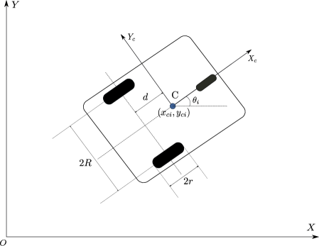
(a)

Figure 2: Robot Model

$$\left[\begin{array}[]{c}\dot{x}_{i}\\ \dot{y}_{i}\\ \dot{\theta}_{i}\end{array}\right]=\left[\begin{array}[]{cc}\mbox{cos}(\theta_{i})&-d.\mbox{sin}(\theta_{i})\\ \mbox{sin}(\theta_{i})&d.\mbox{cos}(\theta_{i})\\ 0&1\end{array}\right]\left[\begin{array}[]{c}u_{i}\\ \omega_{i}\end{array}\right]$$ (27)

Here, $p_{i}=(x_{i},y_{i})^{\scriptscriptstyle\top}$ is the position of the centre point of robot $i$ (this corresponds to the point which is tracked by the localization system). $\theta_{i}$ is the orientation of robot $i$. The control input is given by $v_{i}=(u_{i},\omega_{i})^{\scriptscriptstyle\top}$ where $u_{i}$ and $\omega_{i}$ are the linear and angular velocity commands. $d$ is the distance of the centre point from the wheel axis.

4.2 Adaptive Control Law

The control law derivation is similar to that in Schwager et al. (2009); Abdul Razak et al. (2018). We denote the estimate of parameter $a$ of agent $i$ at time $t$ by $\hat{a}_{i}(t)$ and the measurement of $\phi(.)$ by the agent $i$ by $\phi_{i}(t)=\phi(p_{i}(t))$ where $p_{i}(t)$ is the position of agent $i$ at time $t$. Now we define the following filters:

$$\dot{\Lambda}_{i}(t) =-\alpha\Lambda_{i}(t)+\mathcal{K}_{i}(t)\mathcal{K}_{i}(t)^{\scriptscriptstyle\top}$$ (28)

$$\dot{\lambda}_{i}(t) =-\alpha\lambda_{i}(t)+\mathcal{K}_{i}(t)\phi_{i}(t)$$ (29)

where $\mathcal{K}_{i}(t)=\mathcal{K}(p_{i}(t))$, $\Lambda_{i}(0)={0}$, $\lambda_{i}(0)={0}$.

The control and adaptation laws are then given by

$$v_{i} =-k_{1}\left[S_{i}(q)\right]^{-1}(p_{i}-\hat{C}_{\mathcal{V}_{i}}^{\lambda})$$ (30)

$$\dot{\hat{a}}_{i} =\Gamma(b_{i}-I_{\beta_{i}}b_{i})$$ (31)

$$b_{i} =-k_{2}\int_{\mathcal{V}_{i}}e^{-\frac{\|p_{i}-q\|^{2}}{\sigma^{2}}}\mathcal{K}(q)(q-p_{i})^{T}dq\,\,S_{i}(q)v_{i}$$ (32)

$$\qquad-\gamma(\Lambda_{i}\hat{a}_{i}-\lambda_{i})$$

where $k_{1},k_{2}>0$ are positive gains, $S(q)$ is the matrix

$$\centering S(q)=\left[\begin{array}[]{cc}\mbox{cos}(\theta_{i})&-d.\mbox{sin}(\theta_{i})\\ \mbox{sin}(\theta_{i})&d.\mbox{cos}(\theta_{i})\end{array}\right]\@add@centering$$ (33)

We can now state the following theorem:

Theorem 4.1

Consider $N$ differential drive robots deployed in the region $\mathcal{Q}$ for covering the region. Assume that the robots implement the control law (30) and the adaptation law (31) and (32). Then the following statements hold:

1. $\lim_{t\to\infty}\|p_{i}-\hat{C}_{\mathcal{V}_{i}}^{\lambda}\|=0$,

2. $\lim_{t\to\infty}\|v_{i}\|=0$,

3. $\lim_{t\to\infty}\mathcal{K}_{i}(\tau)\tilde{a}_{i}(t)=0$ for $\forall\tau\,\,\mbox{s.t}\,\,\,t-T<\tau<t$, where $T>0$.

for all $i=1,2,\dots,N$.

Proof

Consider the lyapunov function

$$V=d_{2}(\phi,f_{P})+\frac{1}{2}\sum_{i=1}^{N}\tilde{a}_{i}^{\scriptscriptstyle\top}\Gamma^{-1}\tilde{a}_{i}$$

Taking the derivative,

$$\dot{V} =\sum_{i=1}^{N}\frac{\partial d_{2}}{\partial p_{i}}^{\scriptscriptstyle\top}\dot{p}_{i}+\sum_{i=1}^{N}\tilde{a}_{i}^{\scriptscriptstyle\top}\Gamma^{-1}\dot{\hat{a}}_{i}$$

Using (21), we get

$$\dot{V} =\sum_{i=1}^{N}\frac{4\gamma}{\sigma^{2}}M_{\mathcal{V}_{i}}^{\lambda}(p_{i}-C_{\mathcal{V}_{i}}^{\lambda})^{\scriptscriptstyle\top}\dot{p}_{i}+\sum_{i=1}^{N}\tilde{a}_{i}^{\scriptscriptstyle\top}\Gamma^{-1}\dot{\hat{a}}_{i}$$

Using the definitions of $M_{\mathcal{V}_{i}}^{\lambda}$ and $C_{\mathcal{V}_{i}}^{\lambda}$,

$$\dot{V} =\frac{4\gamma}{\sigma^{2}}\sum_{i=1}^{N}\int_{\mathcal{V}_{i}}(p_{i}-q)^{\scriptscriptstyle\top}\lambda_{i}(q)dq\,\dot{p}_{i}+\sum_{i=1}^{N}\tilde{a}_{i}^{\scriptscriptstyle\top}\Gamma^{-1}\dot{\hat{a}}_{i}$$ (34)

Now $\lambda_{i}(q)$ can be written as

$$\lambda_{i}(q) =e^{-\frac{\|p_{i}-q\|^{2}}{\sigma^{2}}}\left[\phi(q)-\gamma\cdot e^{-\frac{\|p_{i}-q\|^{2}}{\sigma^{2}}}\right]$$

$$=e^{-\frac{\|p_{i}-q\|^{2}}{\sigma^{2}}}\left[\mathcal{K}(q)^{\scriptscriptstyle\top}(\hat{a}_{i}-\tilde{a}_{i})-\gamma\cdot e^{-\frac{\|p_{i}-q\|^{2}}{\sigma^{2}}}\right]$$

$$=e^{-\frac{\|p_{i}-q\|^{2}}{\sigma^{2}}}\left[\hat{\phi}(q)-\gamma\cdot e^{-\frac{\|p_{i}-q\|^{2}}{\sigma^{2}}}\right]$$

$$\quad-\tilde{a}_{i}^{\scriptscriptstyle\top}\mathcal{K}(q)e^{-\frac{\|p_{i}-q\|^{2}}{\sigma^{2}}}$$

$$=\hat{\lambda}_{i}(q)-\tilde{a}_{i}^{\scriptscriptstyle\top}\mathcal{K}(q)e^{-\frac{\|p_{i}-q\|^{2}}{\sigma^{2}}}.$$

where $\hat{\lambda}_{i}(q):=e^{-\frac{\|p_{i}-q\|^{2}}{\sigma^{2}}}\left[\hat{\phi}(q)-\gamma\cdot e^{-\frac{\|p_{i}-q\|^{2}}{\sigma^{2}}}\right]$.
Using this in equation (34), we get

$$\dot{V} =\frac{4\gamma}{\sigma^{2}}\sum_{i=1}^{N}\int_{\mathcal{V}_{i}}(p_{i}-q)^{\scriptscriptstyle\top}\hat{\lambda}_{i}(q)dq\,\dot{p}_{i}+\sum_{i=1}^{N}\tilde{a}_{i}^{\scriptscriptstyle\top}\Gamma^{-1}\dot{\hat{a}}_{i}$$

$$\quad+\frac{4\gamma}{\sigma^{2}}\sum_{i=1}^{N}\tilde{a}_{i}^{\scriptscriptstyle\top}\int_{\mathcal{V}_{i}}\mathcal{K}(q)e^{-\frac{\|p_{i}-q\|^{2}}{\sigma^{2}}}(p_{i}-q)^{\scriptscriptstyle\top}dq\,\dot{p}_{i}$$

Using (27), the control law (30), adaptation law (31) and simplifying, we get

$$\dot{V} =-\frac{4\gamma}{\sigma^{2}}k_{1}\sum_{i=1}^{N}\|p_{i}-\hat{C}_{\mathcal{V}_{i}}^{\lambda}\|^{2}-\sum_{i=1}^{N}\tilde{a}_{i}^{\scriptscriptstyle\top}I_{\beta_{i}}b_{i}$$

$$\quad-\tilde{a}_{i}^{\scriptscriptstyle\top}\int_{0}^{t}e^{-\alpha(t-\tau)}\mathcal{K}_{i}(\tau)\mathcal{K}_{i}(\tau)^{\scriptscriptstyle\top}d\tau\,\tilde{a}_{i}.$$

It can be shown that all three terms of $\dot{V}$ above are non-positive [see Schwager et al. (2009)]. Since $V$ is bounded below by zero and its time derivative is non-positive, it follows that $\lim_{t\to\infty}V(t)$ is finite. This implies that $\dot{V}$ is integrable. Using Barbalat’s lemma, we can conclude that $\lim_{t\to\infty}\dot{V}=0$. Statements 1 and 3 of the theorem follow immediately. Statement 2 follows from statement 1 and equation (30). The proof is thus complete.

Remark 5

From the statements of theorem 4.1, we also observe that $\lim_{t\to\infty}\dot{\theta}_{i}=0$ for all $i=1,2,\dots,N$.

Remark 6

Since we intend to compare the performance of the $\mathcal{L}^{2}$ framework with the locational optimization problem, we mention below the control and adaptation laws for the locational optimization case [see Abdul Razak et al. (2018) for more details on the same] which is derived similar to theorem 4.1.

$$v_{i} =-k_{1}\left[S_{i}(q)\right]^{-1}(p_{i}-\hat{C}_{\mathcal{V}_{i}})$$ (35)

$$\dot{\hat{a}}_{i} =\Gamma(b_{i}-I_{\beta_{i}}b_{i})$$ (36)

$$b_{i} =-k_{2}\int_{\mathcal{V}_{i}}\mathcal{K}(q)(q-p_{i})^{T}dq\,\,S_{i}(q)v_{i}$$ (37)

$$\qquad-\gamma(\Lambda_{i}\hat{a}_{i}-\lambda_{i})$$

4.3 Consensus for improving Parameter Convergence

From the proof of theorem 4.1, it can be observed that the parameter estimate of $\hat{a}_{i}$ converges to the true value $a$ if the matrix

$$\lim_{t\to\infty}\int_{0}^{t}e^{-\alpha(t-\tau)}\mathcal{K}_{i}(\tau)\mathcal{K}_{i}(\tau)^{\scriptscriptstyle\top}d\tau$$

is positive definite. In Schwager et al. (2009), a consensus term was proposed to be included in the adaptation law to improve parameter convergence. It was shown that using a consensus term in the adaptation law makes the parameter estimates of the agents converge to a common value and thus also weakens the sufficient richness condition required for parameter convergence. The modified adaptation law is given by:

$$\dot{\hat{a}}_{i} =\Gamma\left(b_{i}-I_{\beta}b_{i}\right)$$ (38)

$$b_{i} =-F_{i}(p_{i})-\gamma(\Lambda_{i}\hat{a}_{i}-\lambda_{i})-\zeta\sum_{j=1}^{N}l_{ij}(\hat{a}_{i}-\hat{a}_{j})$$ (39)

where $F_{i}(p_{i})$ is the integral term in the adaptation law. The underlying graph used for consensus is the delaunay graph where the agents which share an edge of voronoi partition have the corresponding coefficients $l_{ij}$ non-zero. In Schwager et al. (2009) the authors propose that $l_{ij}$ be equal to the length of the shared voronoi edge ($|\mathcal{V}_{i}\cap\mathcal{V}_{j}|$) between agent $i$ and $j$. An important consequence of using consensus based adaptation law is [see Schwager et al. (2009)].

Corollary 1 (Corollary 2, Schwager et al. (2009))

Using the consensus adaptation law, in addition to the convergence of position and velocity, if the agent paths are such that

$$\sum_{i=1}^{N}\int\limits_{0}^{t}e^{-\alpha(t-\tau)}\mathcal{K}_{i}(\tau)\mathcal{K}_{i}(\tau)^{\scriptscriptstyle\top}d\tau$$

is positive definite, each agent’s parameter estimate converges to the true value of the parameter.

The above condition is weaker since with consensus, the positive definiteness condition is over sum of trajectories of all agents as opposed to the individual trajectories for each of the agents.

4.3.1 Directed Consensus

It can be seen that the agents whose trajectories follow a certain path estimates certain parameters to large accuracy whereas for other parameters they have poor estimates. This can be observed from the adaptation term $-(\Lambda_{i}\hat{a}_{i}-\lambda_{i})$ which means that the error between the measured and the estimated value of $\phi(.)$ is weighted by the corresponding regressor element $\mathcal{K}_{i}^{(j)}$ for updating the corresponding parameter estimate $\hat{a}_{i}^{(j)}$. Thus if the agent trajectory is such that the regressor element always takes a low value, then the corresponding parameter estimate is also very poor. This means that using a consensus term can sometimes reduce the accuracy and/or convergence speed of parameter estimates of those agents which are otherwise able to accurately estimate the parameter.

Based on the above observation, we propose a modified consensus law. Corresponding to each parameter $a^{(j)}$, we construct a directed sub-graph $\mathcal{G}^{(j)}(t)$ of the delaunay graph $\mathcal{G}(t)$ as follows: a directed edge between voronoi neighbours $i$ and $l$ exists if

$$\mathcal{K}_{i}^{(j)}(t)\geq\mathcal{K}_{l}^{(j)}(t).$$ (40)

The weights for the directed edges are taken as constant. This protocol creates a seperate directed sub-graph of the undirected delaunay graph corresponding to each parameter at each time $t$. An illustration is shown in figure 3.

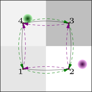
Figure 3: Illustration of directed graphs for consensus: $4$ agents with $2$ parameters - the peak of the basis functions are shown in color with the directed graph for the corresponding parameter shown in the same color; the black color shows the original delaunay graph.

Lemma 3

If the delaunay graph $\mathcal{G}(t)$ is connected and the basis functions in $\mathcal{K}(\cdot)$ are radial functions (i.e., the functions have their peak value at some point and the value reduces with distance from that point), then the directed graphs $\mathcal{G}^{(j)}(t)$ for each $j$ has a rooted tree. The root of the tree is the agent having the maximum value of $\mathcal{K}_{i}^{(j)}(t)$ among all agents $i=1,2,\dots,N$.

Proof

For any $j$ and each pair of agents $(i,l)$ which are voronoi neighbours, we see from condition (40) that there is always a directed edge either from $i$ to $l$ or from $l$ to $i$. Then the agent with the largest value of $\mathcal{K}_{i}^{(j)}(t)$, say $n_{j}$, will only have outgoing edges, and the agent with the smallest value of $\mathcal{K}_{i}^{(j)}(t)$ will only have incoming edges. Given any node (agent) $l$, there always exists atleast one path in the delaunay graph $\mathcal{G}(t)$ (since $\mathcal{G}(t)$ is connected) from agent $n_{j}$ to $l$. In particular, there exists a path such that the sequence of nodes starting from $n_{j}$ in the path are in decreasing order with respect to the value of $\mathcal{K}^{j}(\cdot)$, i.e., $\mathcal{K}^{j}(p_{n_{j}})\geq\dots\geq\mathcal{K}^{j}(p_{l})$. This assertion can be proved as follows: Given node $n_{j}$, either $n_{j}$ is connected to $l$, or it is not. If it is connected, we are done. If it is not connected, there exists another node which is at lower distance from node $n_{j}$ as compared to node $l$. This new node is either connected to $l$, or there has to exist another node which is at smaller distance from this new node as compare to node $l$. This can be continued until all such nodes are exhausted. If all such nodes are exhausted, and the node $l$ is still not connected to one of these nodes, it means that the graph is disconnected which is not possible. Thus there exists some sequence of nodes in increasing order of distance from the node $n_{j}$. This along with the fact that the functions $\mathcal{K}^{j}(\cdot)$ are radial proves the assertion. Using (40) it easily follows that in the directed graph $\mathcal{G}^{(j)}(t)$, there always exists a directed path from the root node $n_{j}$ to any other node. This completes the proof.

Now we modify the adaptation law with each parameter $j$ having seperate consensus law according to the directed sub-graph $\mathcal{G}^{(j)}(t)$. Thus we have the following adaptation law for agent $i$’s parameter estimate:

$$b_{i} =-F_{i}(p_{i})-\gamma(\Lambda_{i}\hat{a}_{i}-\lambda_{i})-\zeta\sum_{j=1}^{N}L_{ij}(\hat{a}_{i}-\hat{a}_{j})$$ (41)

$$=-F_{i}(p_{i})-\gamma(\Lambda_{i}\hat{a}_{i}-\lambda_{i})-\sum_{\alpha=1}^{p}\zeta\sum_{j=1}^{N}l_{ij}^{\alpha}\left(\hat{a}_{i}^{(\alpha)}-\hat{a}_{j}^{(\alpha)}\right)$$ (42)

where $L_{ij}=\mbox{diag}(\{l_{ij}^{\alpha}\}_{\alpha=1}^{p})$ and $L^{\alpha}=\left[l_{ij}^{\alpha}\right]$ is the laplacian matrix for graph $\mathcal{G}^{(\alpha)}(t)$.

Theorem 4.2

Using the modified adaptation law 42, and assuming that all the other conditions of thereom 4.1 hold, all the statements of the theorem 4.1 hold. In addition

$$\lim_{t\to\infty}(\hat{a}_{i}(t)-\hat{a}_{j}(t))=0,$$ (43)

for all $i,j\in\{1,2,\dots,N\}$.

Proof

Proceeding the same way as in the proof of theorem 4.1, we have an additional term in the derivative of the lyapunov function $\dot{V}$, all other terms remaining exactly the same. The term is given by

$$T=-\sum_{i=1}^{N}\tilde{a}_{i}^{\scriptscriptstyle\top}\sum_{j=1}^{N}L_{ij}(\hat{a}_{i}-\hat{a}_{j}).$$

Simplifying this, we have

$$T =\sum_{i=1}^{N}\left[\tilde{a}_{i}^{(1)}\tilde{a}_{i}^{(2)}\dots\tilde{a}_{i}^{(p)}\right]\sum_{j=1}^{N}L_{ij}\left[\begin{array}[]{c}\hat{a}_{i}^{(1)}-\hat{a}_{j}^{(1)}\\ \hat{a}_{i}^{(2)}-\hat{a}_{j}^{(2)}\\ \vdots\\ \hat{a}_{i}^{(p)}-\hat{a}_{j}^{(p)}\end{array}\right]$$

$$=\sum_{\alpha=1}^{p}\sum_{i=1}^{N}\sum_{j=1}^{N}\tilde{a}_{i}^{(\alpha)}l_{ij}^{\alpha}(\hat{a}_{i}^{(\alpha)}-\hat{a}_{j}^{(\alpha)})$$

$$=\sum_{\alpha=1}^{p}\left[\tilde{a}_{1}^{(\alpha)}\dots\tilde{a}_{N}^{(\alpha)}\right]\left[\begin{array}[]{cccc}\sum_{i=2}^{N}l_{1i}^{\alpha}&\dots&\dots&-l_{1N}^{\alpha}\\ -l_{21}^{\alpha}&\dots&\dots&-l_{2N}^{\alpha}\\ \vdots&\vdots&\vdots&\vdots\\ -l_{N1}^{\alpha}&\dots&\dots&\vdots\end{array}\right]\left[\begin{array}[]{c}\hat{a}_{1}^{(\alpha)}\\ \hat{a}_{2}^{(\alpha)}\\ \vdots\\ \hat{a}_{N}^{(\alpha)}\end{array}\right]$$

$$=\sum_{\alpha=1}^{p}\tilde{a}^{{\alpha}^{\scriptscriptstyle\top}}L^{\alpha}\hat{a}^{\alpha}=\sum_{\alpha=1}^{p}\hat{a}^{{\alpha}^{\scriptscriptstyle\top}}L^{\alpha}\hat{a}^{\alpha}$$

where $\hat{a}^{\alpha}=\left[\hat{a}_{1}^{(\alpha)}\,\hat{a}_{2}^{(\alpha)}\,\dots\hat{a}_{N}^{(\alpha)}\right]^{\scriptscriptstyle\top}$.

Thus the term contributed by the consensus term in $\dot{V}$ is non-positive. The term is also uniformly continuous. The other terms in $\dot{V}$ remain non-positive and uniformly continuous as in the proof of theorem 4.1. Thus using Barbalat’s lemma, all the statements of the theorem 4.1 holds. In addition, we have that $\lim_{t\to\infty}\hat{a}^{{\alpha}^{\scriptscriptstyle\top}}L^{\alpha}\hat{a}^{\alpha}=0$ for each $\alpha$. Since $L^{\alpha}$ is the laplacian matrix of the directed graph $\mathcal{G}^{(\alpha)}$, we have that $\lim_{t\to\infty}\hat{a}^{\alpha}=c_{\alpha}\mathbf{1}$ for each $\alpha$ ($c_{\alpha}$ is some positive constant), i.e. the agents achieve consensus on the parameter values and the theorem holds.

5 Hardware Implementation and Experimental Results

In this section, we discuss the details of hardware implementation as well as the experimental results.

5.1 Experiment Setup

The experimental setup consists of five differential drive robots, based on the turtlebot3 platform, with OpenCR 1.0 controller module and Raspberry Pi 3 module mounted on each of them.

5.1.1 Workspace and Localization System

The workspace where the robots move is a flat $4\mbox{m}\times 4\mbox{m}$ square region. For localization of robots, we use the motion-capture system from Optitrack. The system comprises of 16 cameras with infrared sensors which detect the markers fixed atop the robots. A proprietary software (Motive, by Optitrack) uses data in the form of images captured by the cameras, performs localization computations, and provides position data for all the robots in the workspace. This data is streamed over the local network using the Virtual Reality Peripheral Network (VRPN) protocol. The localization system provides millimeter-level precision at high frequencies upto 200 Hz. See figure 4 for the overall setup.

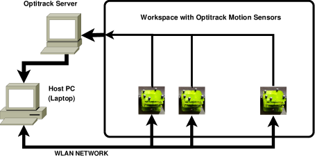
Figure 4: Experiment Setup

The robots communicate with the host PC via WLAN. ROS (Robot Operating System) is used for the software implementation. Each robot runs multiple ROS nodes which implements the coverage algorithm, receives localization data from the Optitrack system as well as communicate with other robots. The host PC runs the ROS master node and subscribes to the position data from the localization system (using VRPN protocol) which are then distributed to the individual robots. Figure 5 shows the overall software implementation using ROS.

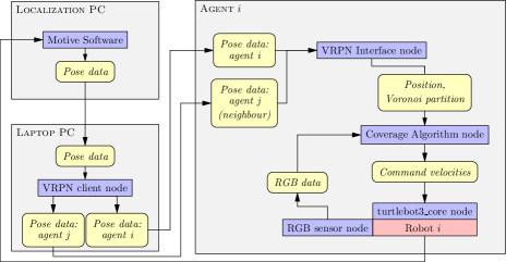
Figure 5: ROS Implementation: the blue blocks represent ROS nodes and the yellow blocks represent the data exchanged between nodes.

5.1.2 Sensors

The density function is implemented as a light distribution using Xiaomi smart bulbs. The Adafruit TCS34725 RGB sensors are used for measuring the light intensity.

5.2 Experimental Results

We do two sets of experiments: (1) The density function is simulated, and (2) the density function is implemented using white light sources, and the agents measure the light intensity using light sensors.
The simulated density function case allows us to study the performance of the coverage algorithm and parameter convergence in better detail since there is no sensor noise and associated issues. Implementing actual sources and sensors allows us to evaluate how well the algorithms behave in the real world with noisy sensors. The values of various constants used in the simulation are given in table 1.

Parameter	Value	Description
Domain related
borderx	[-2.0, 2.0, 2.0, -2.0]	x-coordinates of vertices of the domain
bordery	[-2.0, -2.0, 2.0, 2.0]	y-coordinates of vertices of the domain
Density function related
centrex	[1.0, 1.0]	x-coordinates of centres of density fcn.
centrey	[0.98, -0.8]	y-coordinates of centres of density fcn.
$\sigma$	[0.6, 0.3]	std. deviation
$a$	[85, 30]	true strengths to be estimated
Control and Adaptation gains
$k_{1}$	$0.1$	controller gain
$\Gamma$	$0.1I$	adaptation gain matrix
Loop rates
Control loop	$10$ Hz.	rate at which control loop runs
Position update loop	$20$ Hz.	rate at which position data is available
Robot related
$d$	$0.05$ m	distance of the centre from wheel axis
Adaptation law related
paramInitValue	10	initial value of parameter estimates
$\alpha$	1.0	filter parameter
$\gamma$	2	measurement update gain
$\zeta$	1	consensus related gain

Table 1: Experiment related parameters

5.2.1 Simulated Density Function

The true density function consists of two gaussian components. The various constants related to the density function are given in table 1. The trajectories, average position error and the average velocity of the agents are shown in figure 6. The average position and velocity errors are given by

$$e_{p} =\sum_{i=1}^{N}\|p_{i}-\hat{C}_{\mathcal{V}_{i}}\|,\qquad e_{v}=\sum_{i=1}^{N}\|v_{i}\|.$$

The corresponding plots for the locational optimization based coverage is also shown in the figure for comparison. The initial position error and velocity are higher for the locational optimization case. The agent parameter estimation errors are compared in figures 7 and 8 for the two parameters. It can be seen that for three of the agents the estimation errors for parameter $1$ drops significantly from the initial value, with one agent able to estimate parameter $1$ accurately. The other two agents are not able to adapt for parameter $1$. Similarly two of the agents are able to estimate parameter $2$ better while for the rest of the agents the parameter $2$ estimation error barely change from the initial estimation error. It also appears that the $\mathcal{L}^{2}$ algorithm performs slightly better from figure 7. This could be due to the fact that the integral term in the $\mathcal{L}^{2}$ adaptation law (32) is much smaller (due to the presence of the exponential term) than for the locational optimization adaptation law (37). This term can be viewed as a coupling term between the coverage task (through the cost function $d_{2}(\cdot)$) and the estimation task. The term being smaller means that the estimate $\hat{a}_{i}$ is better able to adapt through the measured error in $\phi(\cdot)$ given by the second term in the adaptation law (32). The parameter errors for adaptation with the consensus terms are shown in figures 9 and 10. We show the average parameter estimation errors across all the agents for ease of comparison since the agent estimation errors closely follow each other due to the consensus term. From the plots we see that overall, the parameter errors starts dropping faster in the locational optimization case although towards the end the drop in error becomes slower compared to the $\mathcal{L}^{2}$ case. This could be due to the fact that the initial velocity is higher for the locational optimization case and thus it is able to initially move faster to regions where significant measurements are available for adaptation. Overall the final values of parameter estimates are slightly better for the $\mathcal{L}^{2}$ case. It can also be seen that the directional consensus algorithm leads to a significantly faster convergence as opposed to the undirected consensus algorithm.

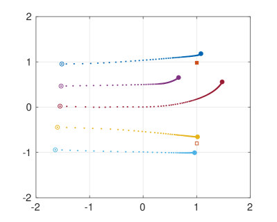
(a) Trajectories

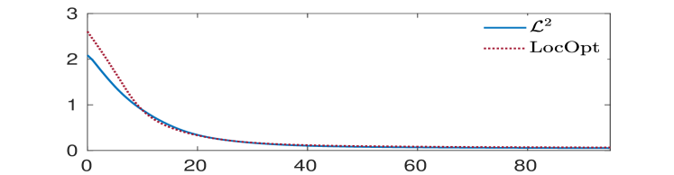
(b) Avg. Position error vs Time (sec).

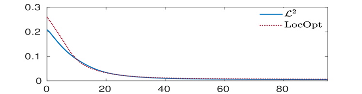
(c) Avg. Velocity vs Time (sec).

Figure 6: Results for $\mathcal{L}^{2}$ coverage: simulated $\phi(\cdot)$.

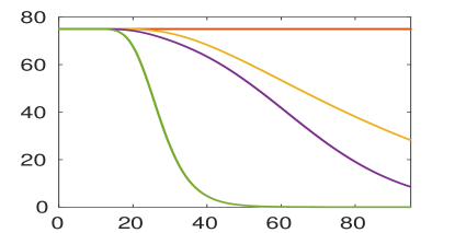
(a) $\mathcal{L}^{2}$ coverage

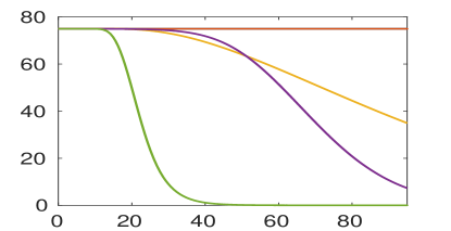
(b) LocOpt coverage

Figure 7: Parameter $1$ estimation errors with time - No consensus.

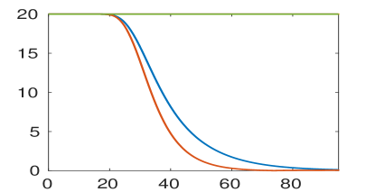
(a) $\mathcal{L}^{2}$ coverage

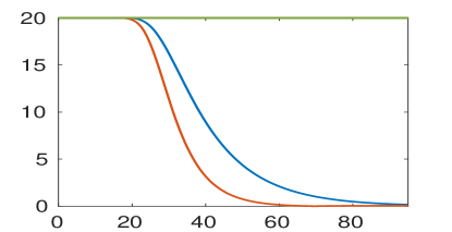
(b) LocOpt coverage

Figure 8: Parameter $2$ estimation errors with time - No consensus.

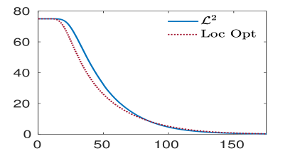
(a) Parameter $1$

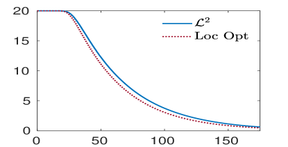
(b) Parameter $2$

Figure 9: Avg. parameter estimation errors with time - with consensus.

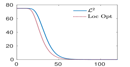
(a) Parameter $1$

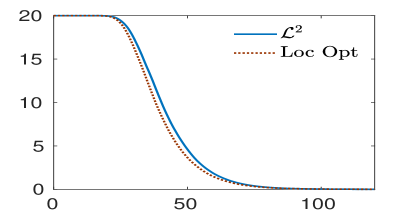
(b) Parameter $2$

Figure 10: Avg. parameter estimation errors with time - with directed consensus.

5.2.2 Density Function implemented using Light Sources

There are two light sources, one of high intensity and the other of lower intensity. Each agent is equipped with TCS34725 RGB sensors to measure the light intensity. The trajectories, average position error and the average velocity of the agents for $\mathcal{L}^{2}$ coverage are shown in figure 11. The plots also show the results of locational optimization based coverage for comparison. As with the results for simulated density function, we see that the initial position error and velocity are larger for the locational optimization case. The agent parameter estimation errors are compared in figures 12 and 13 for the two parameters with no consensus term in the adaptation law. The parameter errors for adaptation with the consensus terms are shown in figures 14 and 15. Overall the parameter estimates using the $\mathcal{L}^{2}$ coverage framework seems to be more accurate. It can also be seen that the direted consensus leads to faster convergence of the parameter errors as expected.

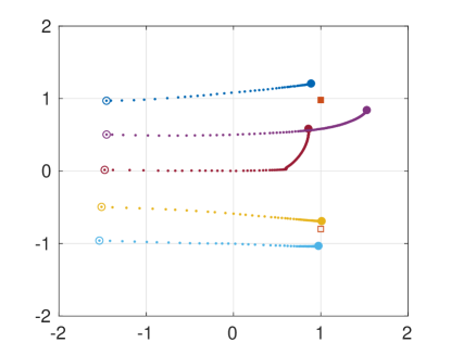
(a) Trajectories

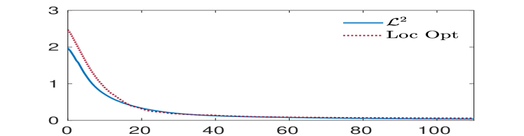
(b) Avg. Position error vs Time (sec).

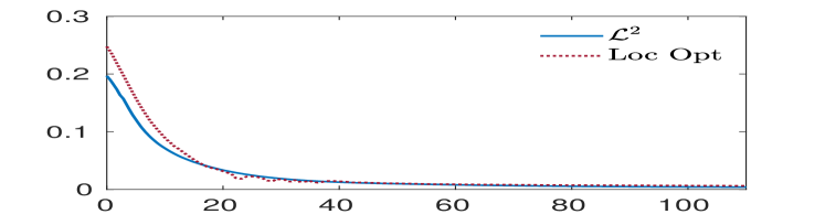
(c) Avg. Velocity vs Time (sec).

Figure 11: Results for $\mathcal{L}^{2}$ coverage: RGB sensors.

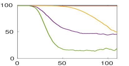
(a) $\mathcal{L}^{2}$ coverage

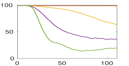
(b) LocOpt coverage

Figure 12: Parameter $1$ estimation errors with time - No consensus.

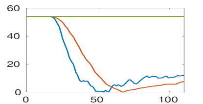
(a) $\mathcal{L}^{2}$ coverage

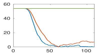
(b) LocOpt coverage

Figure 13: Parameter $2$ estimation errors with time - No consensus.

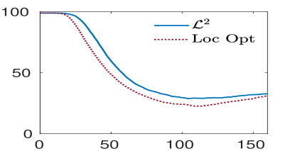
(a) Parameter $1$

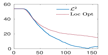
(b) Parameter $2$

Figure 14: Avg. parameter estimation errors with time - with consensus.

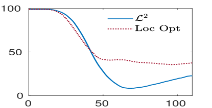
(a) Parameter $1$

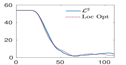
(b) Parameter $2$

Figure 15: Avg. parameter estimation errors with time - with directed consensus.

6 Conclusion

We have looked at an alternative framework for defining the coverage problem. The sensing quality of each agent was quantified as the agent sensing function, and an aggregate sensing function was formed. The coverage problem was then defined as the minimization of some distance between the aggregate function and the density function. We showed that the locational optimization problem can be viewed as a special case of this framework using the K-L divergence as the distance measure. We also looked at the $\mathcal{L}^{2}$ distance as a metric for coverage, and compared the performance of $\mathcal{L}^{2}$ coverage with the locational optimization based coverage.

References

- Abdul Razak et al. (2018) Abdul Razak R, Srikant S, Chung H (2018) Decentralized and adaptive control of multiple nonholonomic robots for sensing coverage. International Journal of Robust and Nonlinear Control 28(6):2636–2650
- Bopardikar et al. (2018) Bopardikar SD, Mehta D, Hauenstein JD (2018) Optimal Configurations in Coverage Control with Polynomial Costs. ArXiv e-prints 1801.10285
- Bullo et al. (2009) Bullo F, Cortés J, Martínez S (2009) Distributed Control of Robotic Networks. Applied Mathematics Series, Princeton University Press, electronically available at http://coordinationbook.info
- Cortes and Bullo (2005) Cortes J, Bullo F (2005) Coordination and geometric optimization via distributed dynamical systems. SIAM Journal on Control and Optimization 44(5):1543–1574
- Cortes et al. (2004) Cortes J, Martinez S, Karatas T, Bullo F (2004) Coverage control for mobile sensing networks. IEEE Trans on Automatic Control 20(2):243–255
- Cortes et al. (May, 2002) Cortes J, Martinez S, Karatas T, Bullo F (May, 2002) Coverage control for mobile sensing networks. In: Proc. IEEE Int. Conf. Robot. Autom., pp 1327–1332
- Flanders (1973) Flanders H (1973) Differentiation Under the Integral Sign. Amer Math Monthly 80(6):615–627
- Guruprasad and Ghose (2013) Guruprasad KR, Ghose D (2013) Heterogeneous locational optimisation using a generalised Voronoi partition. Int J Control 86(6):977–993
- Hexsel et al. (2011) Hexsel B, Chakraborty N, Sycara K (2011) Coverage control for mobile anisotropic sensor networks. In: 2011 IEEE Int. Conf. Robot. and Autom., pp 2878–2885
- Jadbabaie and Lin (2003) Jadbabaie A, Lin J (2003) Coordination of groups of mobile autonomous agents using nearest neighbor rules. IEEE Trans on Automatic Control 48(6):988–1001
- Khalil (2002) Khalil H (2002) Nonlinear Systems. Pearson Education, Prentice Hall
- Kullback and Leibler (1951) Kullback S, Leibler RA (1951) On information and sufficiency. Ann Math Statist 22(1):79–86
- Luna et al. (2013) Luna JM, Fierro R, Abdallah CT, Wood J (2013) An Adaptive Coverage Control for Deployment of Nonholonomic Mobile Sensor Networks Over Time-Varying Sensory Functions. Asian J Control 15(4):988–1000
- Murray (2007) Murray RM (2007) Recent research in cooperative control of multivehicle systems. J Dynam Syst Measur and Control 129(5):571–583
- Olfati-Saber et al. (2007) Olfati-Saber R, Fax A, Murray RM (2007) Consensus and cooperation in networked multi-agent systems. Proceedings of the IEEE 95(1):215–233
- Press (2007) Press W (2007) Numerical Recipes 3rd Edition: The Art of Scientific Computing. Cambridge University Press
- Razak et al. (2018) Razak RA, Sukumar S, Chung H (2018) Distributed coverage control of mobile sensors: Generalized approach using distance functions. In: 2018 IEEE Conference on Decision and Control (CDC), pp 3323–3328
- Schwager et al. (2009) Schwager M, Rus D, Slotine JJ (2009) Decentralized, adaptive coverage control for networked robots. Int J Rob Res 28(3):357–375
- Schwager et al. (Apr. 10-14, 2007) Schwager M, Slotine JE, Rus D (Apr. 10-14, 2007) Decentralized, adaptive control for coverage with networked robots. In: Proc. IEEE Int. Conf. Robot. Autom., pp 3289–3294
- Song et al. (2011) Song C, Feng G, Fan Y, Wang Y (2011) Decentralized adaptive awareness coverage control for multi-agent networks. Automatica 47(12):2749–2756
- Song et al. (2013) Song C, Liu L, Feng G, Wang Y, Gao Q (2013) Persistent awareness coverage control for mobile sensor networks. Automatica 49(6):1867–1873
- Tanner et al. (2007) Tanner H, Jadbabaie A, Pappas G (2007) Flocking in fixed and switching networks. IEEE Trans on Automatic Control 52(5):863–868