On the tension between growth rate and CMB data

Abstract

We analyze the claimed tension between redshift space distorsions measurements of $f(z)\sigma_{8}(z)$ and the predictions of standard $\Lambda$CDM (Planck 2015 and 2018) cosmology. We consider a dataset consisting of 17 data points extending up to redshift $z=1.52$ and corrected for the Alcock-Paczynski effect. Thus, calculating the evolution of the growth factor in a $w$CDM cosmology, we find that the tension for the best fit parameters $w$, $\Omega_{m}$ and $\sigma_{8}$ with respect to the Planck 2018 $\Lambda$CDM parameters is below $2\sigma$ in all the marginalized confidence regions.

I Introduction

Large-scale galaxy surveys are becoming one of the most powerful tools to test the currently accepted $\Lambda$CDM model based on General Relativity. The possibility of mapping the distribution of matter in large volumes at different redshifts allows to measure the growth rate of structures as a function of time and (length) scale which is a well-defined prediction of any cosmological model.

The ability of such surveys to construct 3D maps depends crucially on the precise determination of galaxy redshifts from which radial distances to the survey objects can be inferred. The actual conversion depends, in turn, on two important effects. On one hand, peculiar velocities introduce distorsions in the redshift distribution, the so called redshift space distorsions (RSD), generating an anisotropic galaxy power spectrum. On the other, although at low redshift the Hubble law provides a straightforward relation between resdhift and distances, at higher redshifts this conversion depends on the chosen fiducial cosmology. This fact lays behind the Alcock-Paczynski (AP) effect. In recent times these effects have allowed to measure the linear growth rate of structures, defined as $f=d\ln\delta_{m}/d\ln a$ with $\delta_{m}$ the linear matter density contrast with relatively good precision in a wide range of redshifts. More precisely, RSD provide a measurement of the quantity $f(z)\sigma_{8}(z)$, where $\sigma_{8}(z)$ is the normalization of the linear matter power spectrum at redshift $z$ on scales of $8h^{-1}$Mpc. In particular, measurements which can reach $10\%$ precision have been obtained at $z<1$ by different surveys such as 2dF Percival:2004fs , 6dFGRS Beutler:2012px , WiggleZ Blake:2011rj and recently by SDSS-III BOSS Alam:2016hwk and VIPERS Pezzotta:2016gbo . At higher redshifts two measurements have also been obtained recently by FMOS Okumura:2015lvp and from the BOSS quasar sample Zarrouk:2018vwy although with relatively lower precision.

Confrontation of $f(z)\sigma_{8}(z)$ measurements with standard $\Lambda$CDM cosmology predictions has lead in recent years to claims of inconsistency or tension at different statistical significance levels. Thus in Macaulay:2013swa a lower growth rate than expected from Planck $\Lambda$CDM cosmology was identified for the first time. Later on MacCrann:2014wfa ; Battye:2014qga a tension at the 2$\sigma$ level was claimed between the Planck data and the CFHTLenS determination of $\sigma_{8}$. A similar tension was found by the KiDS+VIKING tomographic shear analysis Hildebrandt:2018yau . More recently Nesseris:2017vor a 3$\sigma$ tension with respect to the best fit parameters of Planck 2015 was also identified in a set of 18 data points from RSD measurements of $f(z)\sigma_{8}(z)$. The tension could even increase up to $5\sigma$ if an extended dataset is used Kazantzidis:2018rnb . The extended dataset has far more data at low redshifts where the model discrimination is easier Kazantzidis:2018jtb , however in this extended case possible correlations within data points have not been taken into account. The possibility that more recent datapoints with larger errorbars compared to earlier datapoints could introduce a bias towards the expected standard Planck/$\Lambda$CDM cosmology is also discussed in Kazantzidis:2018rnb .

In this paper, we follow a complementary approach, rather than using the extended dataset for which correlations are unknown, we will revisit the analysis of the tension from the most conservative point of view, i.e. using only independent datapoints or points whose correlations are known. Thus we consider the Gold dataset of Nesseris:2017vor and introduce two changes in the analysis. Firstly, we include the most recent measurements from BOSS-Q Zarrouk:2018vwy and on the other, we draw attention on the possible correlation between SDSS-LRG and BOSS-LOWZ points. Notice that the former are obtained from the SDSS data release DR7 with practically the same footprint as the later, obtained from DR10 and DR11, but with less galaxies. In this sense, we explore the consequences of removing the two SDSS-LRG points from the analysis. In this sense, our dataset is very similar to that consider by Planck collaboration Aghanim:2018eyx . On the other hand, we will take the best fit parameters of Planck 2018 (CMB alone) given in Aghanim:2018eyx rather than Planck 2015 used in Nesseris:2017vor . We consider the same type of $w$CDM cosmologies with three free parameters $(w,\Omega_{m},\sigma_{8})$ but obtain the confidence regions from the marginalized (rather than maximized) likelihoods. This enlarges the confidence regions so that the tension is found to be reduced below the $2\sigma$ level for all the parameters combinations.

II Growth of structures and $f(z)\sigma_{8}(z)$

Let us consider a flat Robertson-Walker background whose metric in conformal time reads

$$ds^{2}=a^{2}(\eta)\left[-d\eta^{2}+\delta_{ij}dx^{i}dx^{j}\right]$$ (1)

The evolution of matter density perturbations $\delta_{m}=\delta\rho_{m}/\rho_{m}$ in a general cosmological model with non-clustering dark energy and standard conservation of matter is given for sub-Hubble scales by

$$\delta_{m}^{\prime\prime}+\mathcal{H}\delta_{m}^{\prime}-\frac{3}{2}\mathcal{H}^{2}\Omega_{m}(a)\delta_{m}=0$$ (2)

where prime denotes derivative with respect to conformal time, ${\cal H}=a^{\prime}/a$ and $\Omega_{m}(a)=\rho_{m}/(\rho_{m}+\rho_{DE})$. In this work we will limit ourselves to $w$CDM cosmologies so that at late times

$${\cal H}^{2}=H_{0}^{2}a^{2}(\Omega_{m}a^{-3}+(1-\Omega_{m})a^{-3(1+w)})$$ (3)

and

$$\Omega_{m}(a)=\frac{\Omega_{m}}{\Omega_{m}+(1-\Omega_{m})\ a^{-3w}}$$ (4)

The growth rate is defined as

$$f=\frac{d\ln\delta_{m}}{d\ln a}$$ (5)

which can be approximated by $f\simeq\Omega_{m}^{\gamma}(a)$ with $\gamma\simeq 0.55$ for $w$CDM models. Even though this fitting function provides accurate description for cosmologies close to $\Lambda$CDM, since we are interested in exploring a wide range of parameter space, in this work we will obtain $f$ just by numerically solving (2) with initial conditions $\delta_{m}(a_{i})=1$ and $\delta^{\prime}(a_{i})=1/a_{i}$ with $a_{i}$ well inside the matter dominated era.

The matter power spectrum corresponding to the matter density contrast in Fourier space $\delta_{k}(z)$ with $1+z=1/a$ is given by $P(k,z)=V|\delta_{k}(z)|^{2}$ with $V$ the volume. Thus the variance of the matter fluctuations on a scale $R$ is given by

$$\sigma_{R}^{2}(z)=\frac{1}{2\pi^{2}}\int P(k^{\prime},z)W_{R}^{2}(k^{\prime})^{2}dk^{\prime}$$ (6)

with the window function defined as:

$$W_{R}(k)=\frac{3}{k^{3}R^{3}}\,[\sin(kR)-kR\cos(kR)]$$ (7)

Thus $\sigma_{8}(z)$ corresponds to $\sigma_{R}(z)$ at the scale $R=8h^{-1}$ Mpc.

From the matter power spectrum it is possible to define the galaxy power spectrum as $P_{g}(k,z)=b^{2}(z)P(k,z)$ with $b(z)$ the bias factor.

From the observational point of view, galaxy surveys are able to determine the galaxy power spectrum in redshift space, which is given by

$$P_{r,\textrm{obs}}(k_{r},\mu_{r};z)$$

$$= \frac{H(z)d_{Ar}^{2}(z)}{H_{r}(z)d_{A}^{2}(z)}D^{2}(z)b^{2}(z)\left[1+\beta(z)\mu^{2}\right]^{2}P(k,z=0)$$

where $H(z)=(1+z){\cal H}(z)$,

$$d_{A}(z)=\frac{1}{1+z}\int_{\frac{1}{1+z}}^{1}\frac{1}{a^{1/2}}\frac{da}{H_{0}\sqrt{\Omega_{m}+(1-\Omega_{m})\ a^{-3w}}}$$ (9)

is the angular diameter distance, $D(z)=\delta_{m}(z)/\delta_{m}(0)$ is the growth factor, $\beta(z)=f(z)/b(z)$ and $\mu$ is the cosine of the angle between $\hat{k}$ and the observation direction. Finally, the index $r$ denotes that the corresponding quantity is evaluated on the fiducial cosmology. Notice that the first factor in (II) corresponds to the AP effect, whereas the $(1+\beta\mu^{2})^{2}$ factor is generated by the RSD. As we see RSD induce an angular dependence on the power spectrum which contains a monopole, quadrupole and hexadecapole contributions. From the measurements of monopole and quadropole it is possible to obtain the $f(z)\sigma_{8}(z)$ function that for simplicity in the following we will simple denote $f\sigma_{8}(z)$. The measured value depends on the fiducial cosmology, so that in order to translate from the fiducial cosmology used by the survey to other cosmology it is needed to rescale by a factor Nesseris:2017vor

$$\textrm{ratio}(z)=\frac{H(z)d_{A}(z)}{H_{r}(z)d_{A,r}(z)}$$ (10)

The fiducial cosmology correction could affect not only $f\sigma_{8}$ but also the power spectrum or even introduce additional multipoles in the galaxy power spectrum in redshift space. In principle, all these effects could be properly taken into account but, as shown in Kazantzidis:2018rnb , in practice an approximated approach is employed which relies on the introduction of correction factors. In our case, and in order to check the results of Nesseris:2017vor and Kazantzidis:2018rnb , we have chosen the same correction factors used in those references. The same factors were used in Macaulay:2013swa . In any case, different approaches can change the significance of the tension.

III Testing Planck cosmology

In order to confront the predictions of standard $\Lambda$CDM model with $f\sigma_{8}(z)$ measurements, we will obtain theoretical predictions for a general $w$CDM model with three free parameters $(\Omega_{m},w,\sigma_{8})$ with $\sigma_{8}=\sigma_{8}(z=0)$. Our benchmark models will correspond to the Planck 2015 and Planck 2018 (TT,TE,EE+lowE) best fit parameters in Table 1.

	Planck 2015	Planck 2018
$\Omega_{m}$	$0.3156\pm 0.0091$	$0.3166\pm 0.0084$
$w$	$-1$	$-1$
$\sigma_{8}$	$0.831\pm 0.013$	$0.8120\pm 0.0073$

Table 1: Planck 2015 Ade:2015xua and 2018 Aghanim:2018eyx (TT,TE,EE+lowE) best fit $\Lambda$CDM parameters.

On the other hand, our data points will correspond to measurements of SDSS Samushia:2011cs ; Howlett:2014opa ; Feix:2015dla ; 6dFGS Huterer:2016uyq ; IRAS Hudson:2012gt ; Turnbull:2011ty ; $2$MASS Davis:2010sw ; Hudson:2012gt ; 2dFGRS Song:2008qt , GAMA Blake:2013nif , BOSS Sanchez:2013tga , WiggleZ Blake:2012pj , Vipers Pezzotta:2016gbo , FastSound Okumura:2015lvp and BOSS Q Zarrouk:2018vwy . In Table 2 we show the 17 independent data points with the corresponding fiducial cosmology parameters corresponding to the so called Gold-2017 compilation of Nesseris:2017vor which contains 18 robust and independent measurements based on galaxy or SNIa observations together with an additional independent BOSS quasar point. As mentioned before, we have removed the two SDSS-LRG-200 points since they are based on almost the same galaxy selection as the BOSS-LOWZ point from two heavily overlapping footprints with BOSS-LOWZ including fainter galaxies. On the data provided by these surveys we will apply the fiducial cosmology correction given by (10).

Index	Dataset	$z$	$f\sigma_{8}(z)$	$\Omega_{m}$
$1$	6dFGS+SnIa	$0.02$	$0.428\pm 0.0465$	$0.3$
$2$	SnIa+IRAS	$0.02$	$0.398\pm 0.065$	$0.3$
$3$	2MASS	$0.02$	$0.314\pm 0.048$	$0.266$
$4$	SDSS–veloc	$0.10$	$0.370\pm 0.130$	$0.3$
$5$	SDSS-MGS	$0.15$	$0.490\pm 0.145$	$0.31$
$6$	2dFGRS	$0.17$	$0.510\pm 0.060$	$0.3$
$7$	GAMA	$0.18$	$0.360\pm 0.090$	$0.27$
$8$	GAMA	$0.38$	$0.440\pm 0.060$	$0.27$
$9$	BOSS–LOWZ	$0.32$	$0.384\pm 0.095$	$0.274$
$10$	SDSS-CMASS	$0.59$	$0.488\pm 0.060$	$0.307115$
$11$	WiggleZ	$0.44$	$0.413\pm 0.080$	$0.27$
$12$	WiggleZ	$0.60$	$0.390\pm 0.063$	$0.27$
$13$	WiggleZ	$0.73$	$0.437\pm 0.072$	$0.27$
$14$	Vipers PDR–2	$0.60$	$0.550\pm 0.120$	$0.3$
$15$	Vipers PDR–2	$0.86$	$0.400\pm 0.110$	$0.3$
$16$	FastSound	$1.40$	$0.482\pm 0.116$	$0.270$
$17$	BOSS-Q	$1.52$	$0.426\pm 0.077$	$0.31$

Table 2: Data points from Nesseris:2017vor ; Zarrouk:2018vwy .

Apart from the errors quoted in Table 2, the three points corresponding to WiggleZ are correlated. Thus the non-diagonal covariance matrix for the data points $11,12,13$ is given by:

$$C_{ij}^{11,12,13}=10^{-3}\left(\begin{array}[]{ccc}6.4000&2.570&0.000\\ 2.570&3.969&2.540\\ 0.000&2.540&5.184\end{array}\right)$$ (14)

and the total covariance matrix would be

$$C_{ij}=\left(\begin{array}[]{cccc}\sigma_{1}^{2}&0&0&...\\ 0&C_{ij}^{11,12,13}&0&...\\ 0&0&...&\sigma_{N}^{2}\end{array}\right)$$ (18)

The corresponding $\chi^{2}$ is defined as

$$\chi^{2}(\Omega_{m},w,\sigma_{8})=V^{i}C_{ij}^{-1}V^{j}$$ (19)

with $V^{i}=f\sigma_{8,i}-\textrm{ratio}(z_{i})f\sigma_{8}(z_{i};\Omega_{m},w,\sigma_{8})$. Here $f\sigma_{8,i}$ corresponds to each of the data points in Table 2 and $f\sigma_{8}(z_{i};\Omega_{m},w,\sigma_{8})$ is the theoretical value for a given set of parameters values. In order to obtain the two-dimensional confidence regions for the different pairs of parameters, we will construct the marginalized likelihoods integrating the remaining parameter with a flat prior , i.e.

$$L(w,\sigma_{8})=N\int_{\Delta\Omega_{m}}e^{-\frac{1}{2}\chi^{2}(\Omega_{m},w,\sigma_{8})}\,d\Omega_{m}$$ (20)

In particular for $\Omega_{m}\in[0.05;0.9]$, $w\in[-2.5;0.5]$ and $\sigma_{8}\in[0.1;4.0]$. We have checked that the confidence regions remain practically unchanged if we enlarge these intervals. Notice that this is one of the main differences with respect to Nesseris:2017vor in which the remaining parameter was fixed to the Planck cosmology value. This procedure implies the introduction of a strong prior in the likelihood (20) from CMB data. However, if we want to determine the confidence regions obtained from $f\sigma_{8}$ data alone, no CMB information should be included in the corresponding likelihoods which is the approach considered in this work.

IV Results

In Fig. 1, the data points quoted in Table 2 together with the corresponding $w$CDM best fit curve are represented. The best fit corresponds to the parameters $\Omega_{m}=0.145$, $\sigma_{8}=1.18$ and $w=-0.46$. For the sake of comparison we also show the $f\sigma_{8}(z)$ curves corresponding to the Planck $2015$ and Planck $2018$ (in Table 1) cosmologies. The $\chi^{2}$ values for the different models can be found in Table 3 together with the corresponding tension level obtained from the $\chi^{2}$ difference for a three-parameter distribution. As we can see, for both models the tension of Planck cosmology with respect to the best fit $w$CDM cosmology is below 2$\sigma$.

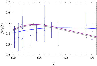
Figure 1: Blue line corresponds to $w$CDM best fit, purple line corresponds to Planck $2015$ and grey line to Planck $2018$.

Model	$\chi^{2}_{LRG}$	$\chi^{2}_{N}$
$w$CDM	16.51	$10.09$
Planck $2015$	21.58 ($1.38\sigma$)	$16.22$ ($1.62\sigma$)
Planck $2018$	18.32 ($0.51\sigma$)	$14.31$ ($1.18\sigma$)

Table 3: Values of $\chi^{2}$ for the models plotted in Fig. 1. $\chi^{2}_{LRG}$ refers to the dataset in Nesseris:2017vor whereas $\chi^{2}_{N}$ refers to the data set in this work in Table 2. The best fit parameters for $w$CDM with $LRG$ data points are $\sigma_{8}=1.57$, $\Omega_{M}=0.1$ and $w=-0.27$. The tension between Planck cosmologies and $w$CDM for three fitted parameters is also shown in parenthesis.

We see that Planck 2018 provides a better fit than the Planck 2015 cosmology, mainly thanks to the reduction in the $\sigma_{8}$ parameter, but still both are well above the best fit to $w$CDM.

In order to obtain the corresponding confidence regions we will compare two procedures. On one hand, we will follow the approach in Nesseris:2017vor in which the likelihood is maximized, i.e. in the two-dimensional confidence regions the remaining parameter is fixed to the corresponding Planck value in Table 1. In the second procedure, the remaining parameter is marginalized as mentioned in the previous section. In Figs. 2, 3 and 4 we show the different two-dimensional confidence contours. As we can see, Planck 2018 $\Lambda$CDM shows tensions of $1.56\sigma$, $1.19\sigma$ and $1.68\sigma$ in the maximized contours which is around $1\sigma$ below the tension found in Nesseris:2017vor with Planck 2015 parameters, partially thanks to the reduced $\sigma_{8}$ value of Planck 2018 as mentioned before and the exclusion of the two SDSS-LRG points. On the other hand, the marginalized contours are as expected enlarged as compared to the maximized ones. Notice also that although the form of the $(\sigma_{8},w)$ and $(\Omega_{m},\sigma_{8})$ contours are similar in both cases, the marginalization procedure changes the shape of the $(\Omega_{m},w)$ regions and the tensions with respect to Planck 2018 are $1.71\sigma$ for $(\Omega_{m},w)$, $0.33\sigma$ for $(\sigma_{8},w)$ and in the $(\Omega_{m},\sigma_{8})$ plane we get $1.23\sigma$. In Table 4 the different tension levels are summarized for the two Planck cosmologies, comparing maximized and marginalized contours and with the dataset in this work and that in Nesseris:2017vor .

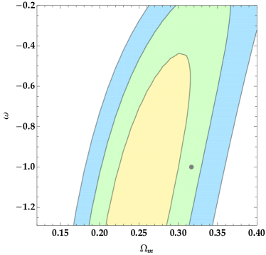
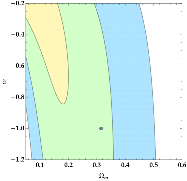
Figure 2: $w$ vs. $\Omega_{m}$ 1$\sigma$, 2$\sigma$ and 3$\sigma$ confidence regions. Left: maximized contours with $\sigma_{8}=0.812$. The Planck $2018$ point lays at $1.56\sigma$. Right: marginalized contours. The blue point corresponds to Planck $2015$ and lays at $1.71\sigma$; and the grey point corresponds to Planck $2018$ and lays also at $1.71\sigma$

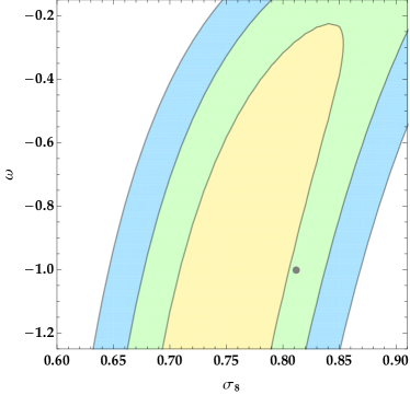
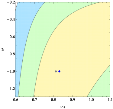
Figure 3: $w$ vs. $\sigma_{8}$ 1$\sigma$, 2$\sigma$ and 3$\sigma$ confidence regions. Left: maximized contours with $\Omega_{m}=0.3166$. The Planck $2018$ point lays at $1.19\sigma$. Right: marginalized contours. The blue point corresponds to Planck $2015$ and lays at $0.26\sigma$ and the grey point corresponds to Planck $2018$ and lays at $0.33\sigma$.

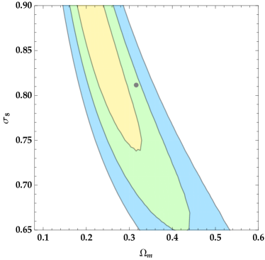
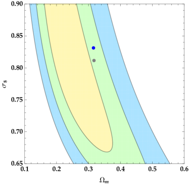
Figure 4: $\sigma_{8}$ vs. $\Omega_{m}$ 1$\sigma$, 2$\sigma$ and 3$\sigma$ confidence regions. Left: maximized contours with $w=-1$. The Planck $2018$ point lays at $1.68\sigma$. Right: marginalized contours. The blue point corresponds to Planck $2015$ and lays at $1.44\sigma$. The grey point corresponds to Planck $2018$ and lays at $1.23\sigma$.

		MaxLRG	MargLRG	MaxN	MargN
$\sigma_{8}$-$w$	P15	$2.70\sigma$	$0.29\sigma$	$1.76\sigma$	$0.26\sigma$
	P18	$2.04\sigma$	$0.30\sigma$	$1.19\sigma$	$0.33\sigma$
$\Omega_{m}$-$w$	P15	$2.86\sigma$	$1.57\sigma$	$2.08\sigma$	$1.71\sigma$
	P18	$2.22\sigma$	$1.58\sigma$	$1.56\sigma$	$1.71\sigma$
$\Omega_{m}$ -$\sigma_{8}$	P15	$2.87\sigma$	$1.50\sigma$	$2.14\sigma$	$1.44\sigma$
	P18	$2.25\sigma$	$1.28\sigma$	$1.68\sigma$	$1.23\sigma$

Table 4: Tension levels for the Planck 2015 and Planck 2018 $\Lambda$CDM cosmologies in the different two-dimensional maximized and marginalized regions for the datasets in Table 2 ($N$) and in Nesseris:2017vor (LRG).

V Conclusions

We have revisited the tension of $\Lambda$CDM Planck cosmology with RSD growth data. We have considered the Gold data set of Nesseris:2017vor together with one additional BOSS-Q point and removing the two SDSS-LRG points thus obtaining a total of 17 independent data points.

Confronting these data with the growth rate obtained from a $w$CDM cosmology with three independent parameters $(w,\Omega_{m},\sigma_{8})$, we find that unlike previous claims, the tension with Planck 2018 cosmology is below the $2\sigma$ level in all the two-dimensional marginalized confidence regions. This reduction, which is around $1.5\sigma$ as compared to Nesseris:2017vor , is due to three different factors, namely, the use of Planck 2018 parameters, the fact that marginalized confidence regions have been considered and the exclusion of the possibly correlated SDSS-LRG points. Notice that for the $\Lambda$CDM model (i.e. fixing $w=-1$), the tension is found to be at $1.68\sigma$ level.

Future galaxy surveys such as J-PAS Benitez:2014ibt , DESI Aghamousa:2016zmz or Euclid Laureijs:2011gra with increased effective volumes will be able to reduce the error bars in the determination of $f\sigma_{8}(z)$ in almost an order of magnitude and will help to confirm or exclude the tension analyzed in this work.

References

- (1) W. J. Percival et al. [2dFGRS Collaboration], Mon. Not. Roy. Astron. Soc. 353 (2004) 1201 doi:10.1111/j.1365-2966.2004.08146.x [astro-ph/0406513].
- (2) F. Beutler et al., Mon. Not. Roy. Astron. Soc. 423 (2012) 3430 doi:10.1111/j.1365-2966.2012.21136.x [arXiv:1204.4725 [astro-ph.CO]].
- (3) C. Blake et al., Mon. Not. Roy. Astron. Soc. 415 (2011) 2876 doi:10.1111/j.1365-2966.2011.18903.x [arXiv:1104.2948 [astro-ph.CO]].
- (4) S. Alam et al. [BOSS Collaboration], Mon. Not. Roy. Astron. Soc. 470 (2017) no.3, 2617 doi:10.1093/mnras/stx721 [arXiv:1607.03155 [astro-ph.CO]].
- (5) A. Pezzotta et al., Astron. Astrophys. 604 (2017) A33 doi:10.1051/0004-6361/201630295 [arXiv:1612.05645 [astro-ph.CO]].
- (6) T. Okumura et al., Publ. Astron. Soc. Jap. 68 (2016) no.3, 38 doi:10.1093/pasj/psw029 [arXiv:1511.08083 [astro-ph.CO]].
- (7) P. Zarrouk et al., Mon. Not. Roy. Astron. Soc. 477 (2018) no.2, 1639 doi:10.1093/mnras/sty506 [arXiv:1801.03062 [astro-ph.CO]].
- (8) E. Macaulay, I. K. Wehus and H. K. Eriksen, Phys. Rev. Lett. 111 (2013) no.16, 161301 doi:10.1103/PhysRevLett.111.161301 [arXiv:1303.6583 [astro-ph.CO]].
- (9) N. MacCrann, J. Zuntz, S. Bridle, B. Jain and M. R. Becker, Mon. Not. Roy. Astron. Soc. 451 (2015) no.3, 2877 doi:10.1093/mnras/stv1154 [arXiv:1408.4742 [astro-ph.CO]].
- (10) R. A. Battye, T. Charnock and A. Moss, Phys. Rev. D 91 (2015) no.10, 103508 doi:10.1103/PhysRevD.91.103508 [arXiv:1409.2769 [astro-ph.CO]].
- (11) H. Hildebrandt et al., arXiv:1812.06076 [astro-ph.CO].
- (12) S. Nesseris, G. Pantazis and L. Perivolaropoulos, Phys. Rev. D 96 (2017) no.2, 023542 doi:10.1103/PhysRevD.96.023542 [arXiv:1703.10538 [astro-ph.CO]].
- (13) L. Kazantzidis and L. Perivolaropoulos, Phys. Rev. D 97 (2018) no.10, 103503 doi:10.1103/PhysRevD.97.103503 [arXiv:1803.01337 [astro-ph.CO]].
- (14) L. Kazantzidis, L. Perivolaropoulos and F. Skara, Phys. Rev. D 99 (2019) no.6, 063537 doi:10.1103/PhysRevD.99.063537 [arXiv:1812.05356 [astro-ph.CO]].
- (15) F. Skara and L. Perivolaropoulos, arXiv:1911.10609 [astro-ph.CO].
- (16) N. Aghanim et al. [Planck Collaboration], arXiv:1807.06209 [astro-ph.CO].
- (17) P. A. R. Ade et al. [Planck Collaboration], Astron. Astrophys. 594 (2016) A13 doi:10.1051/0004-6361/201525830 [arXiv:1502.01589 [astro-ph.CO]].
- (18) L. Samushia, W. J. Percival and A. Raccanelli, Mon. Not. Roy. Astron. Soc. 420 (2012) 2102 doi:10.1111/j.1365-2966.2011.20169.x [arXiv:1102.1014 [astro-ph.CO]].
- (19) C. Howlett, A. Ross, L. Samushia, W. Percival and M. Manera, Mon. Not. Roy. Astron. Soc. 449 (2015) no.1, 848 doi:10.1093/mnras/stu2693 [arXiv:1409.3238 [astro-ph.CO]].
- (20) M. Feix, A. Nusser and E. Branchini, Phys. Rev. Lett. 115 (2015) no.1, 011301 doi:10.1103/PhysRevLett.115.011301 [arXiv:1503.05945 [astro-ph.CO]].
-
(21)
D. Huterer, D. Shafer, D. Scolnic and F. Schmidt,
JCAP 1705 (2017) no.05, 015
doi:10.1088/1475-7516/2017/05/015
[arXiv:1611.09862 [astro-ph.CO]].
-
(22)
M. J. Hudson and S. J. Turnbull,
Astrophys. J. 751 (2013) L30
doi:10.1088/2041-8205/751/2/L30
[arXiv:1203.4814 [astro-ph.CO]].
- (23) S. J. Turnbull, M. J. Hudson, H. A. Feldman, M. Hicken, R. P. Kirshner and R. Watkins, Mon. Not. Roy. Astron. Soc. 420 (2012) 447 doi:10.1111/j.1365-2966.2011.20050.x [arXiv:1111.0631 [astro-ph.CO]].
- (24) M. Davis, A. Nusser, K. Masters, C. Springob, J. P. Huchra and G. Lemson, Mon. Not. Roy. Astron. Soc. 413 (2011) 2906 doi:10.1111/j.1365-2966.2011.18362.x [arXiv:1011.3114 [astro-ph.CO]].
- (25) Y. S. Song and W. J. Percival, JCAP 0910 (2009) 004 doi:10.1088/1475-7516/2009/10/004 [arXiv:0807.0810 [astro-ph]].
- (26) C. Blake et al., Mon. Not. Roy. Astron. Soc. 436 (2013) 3089 doi:10.1093/mnras/stt1791 [arXiv:1309.5556 [astro-ph.CO]].
- (27) A. G. Sanchez et al., Mon. Not. Roy. Astron. Soc. 440 (2014) no.3, 2692 doi:10.1093/mnras/stu342 [arXiv:1312.4854 [astro-ph.CO]].
- (28) C. Blake et al., Mon. Not. Roy. Astron. Soc. 425 (2012) 405 doi:10.1111/j.1365-2966.2012.21473.x [arXiv:1204.3674 [astro-ph.CO]].
- (29) N. Benitez et al. [J-PAS Collaboration], arXiv:1403.5237 [astro-ph.CO].
- (30) A. Aghamousa et al. [DESI Collaboration], arXiv:1611.00036 [astro-ph.IM].
- (31) R. Laureijs et al. [EUCLID Collaboration], arXiv:1110.3193 [astro-ph.CO].