A numerical toolkit for multiprojective varieties
Abstract.
A numerical description of an algebraic subvariety of projective space is given by a general linear section, called a witness set. For a subvariety of a product of projective spaces (a multiprojective variety), the corresponding numerical description is given by a witness collection, whose structure is more involved. We build on recent work to develop a toolkit for the numerical manipulation of multiprojective varieties that operates on witness collections and use this toolkit in an algorithm for numerical irreducible decomposition of multiprojective varieties. The toolkit and decomposition algorithm are illustrated throughout in a series of examples.
Key words and phrases:
numerical algebraic geometry, multiprojective variety2010 Mathematics Subject Classification:
65H10Introduction
Numerical algebraic geometry [20] uses numerical analysis to manipulate and study algebraic varieties on a computer. In numerical algebraic geometry, a subvariety of affine or projective space is represented by a witness set, which includes a finite set of points in a general linear section of [16]. Algorithms to manipulate a variety operate on its witness sets. A fundamental algorithm is numerical irreducible decomposition [17], which uses monodromy [18] and a trace test [19] to partition a witness set of a reducible variety into witness sets for each irreducible component.
Oftentimes, a variety possesses additional structure, such as multihomogeneity, which is when its defining polynomials are separately homogeneous in disjoint subsets of variables. For example, the determinant is separately linear in the variables of each column. Such a variety is naturally a subvariety of a product of projective spaces (a multiprojective variety). For the determinant, this product is ( factors). We seek algorithms for multiprojective varieties that are adapted to their structure.
Algorithms for numerically solving systems of multihomogeneous polynomials are classical [13]. A useful notion of witness set—a witness collection—for multiprojective varieties, along with fundamental algorithms, was given in [6]. There, it was observed that the trace test could not be applied naively to a witness collection. Consequently, for numerical irreducible decomposition, a witness collection for a multiprojective variety must be transformed into a witness set for a projective or affine variety. Since a multiprojective variety is a projective variety under the Segre embedding, that could be used for numerical irreducible decomposition. In general, the Segre embedding dramatically increases the ambient dimension and degree as we show in Section 1.7. Passing instead to an affine patch in the product of projective spaces preserves the ambient dimension, but we do not know an algorithm of acceptable complexity to compute a witness set from a witness collection unless the variety is a curve. This is because for curves the Segre embedding can be used without increasing the degree so much as seen in Section 4.
A version of numerical irreducible decomposition was proposed for subvarieties in the product of two projective spaces [10]. This reduces numerical irreducible decomposition to that of a curve, decreasing the size of the witness sets. We extend that analysis to arbitrary multiprojective varieties. We present four geometric constructions and corresponding algorithms that operate on witness collections, and together provide a toolkit for the numerical manipulation of multiprojective varieties. A key ingredient is the support of a multiprojective variety [2], which is a multiprojective version of dimension.
The computation of this (multi)dimension locally at a point reduces to linear algebra. When the multidimension decomposes as a product, the corresponding variety is also a product as is a witness collection for it. We next explain how witness collections transform under birational maps that change the multiprojective structure, and finally how a witness collection behaves under slicing with a hyperplane. We also give an algorithm based on monodromy for computing a witness collection. The utility of this toolkit is illustrated in an algorithm for numerical irreducible decomposition of multiprojective varieties. We use these tools to reduce the numerical irreducible decomposition to that of a curve in affine space, to which we may apply an efficient trace test. This generalizes the method of [10], from two to arbitrarily many projective factors.
Algorithms in numerical algebraic geometry typically operate on affine varieties. A subvariety of projective space is replaced by its intersection with a general affine patch where a general linear polynomial does not vanish. The same approach could be followed for a multiprojective variety by taking affine patches in each projective factor and combining them, giving . This neglects the given structure and increases the size and complexity of the witness set, which is particularly significant when is neither a curve nor a hypersurface. We will work with multiaffine varieties , using algorithms that respect this decomposition and are compatible with the multiprojective structure of .
This paper is structured as follows. In Section 1, we define witness collections of multiprojective and multiaffine varieties, and introduce some running examples. In Section 2, we give an algorithm to compute (multi)dimension locally and an algorithm based on monodromy to compute a witness collection. In Section 3, we show how to detect and exploit that a variety is a product. In Section 4, we show how to transform witness collections under the birational maps that correspond to changing the multiprojective structure of a variety. In Section 5, we show how to perform a dimension reduction based on intersections with linear spaces that preserves (ir)reducibility. In Section 6, we sketch an algorithm for numerical irreducible decomposition that uses this toolkit. In Section 7, we consider two examples based on fiber products which naturally yield multihomogeneous systems. Apart from showcasing our toolkit, these examples demonstrate that using multiprojective structure leads to significant reduction in the size of computations.
1. Background
For a finite set of polynomials, let be its variety, the subset of affine or projective space (or products thereof) where every polynomial in vanishes. A variety will also be a union of irreducible components of such a set . We first recall numerical homotopy continuation, then witness sets [20, Ch. 13], multiprojective varieties, witness collections [6], and multiaffine varieties. We end by introducing our running examples.
1.1. Numerical homotopy continuation
Many algorithms described herein are based on numerical homotopy continuation. A homotopy is a system of polynomials (, ), that interpolates between two systems—the start system when and the target system when —in a particular way. We require that contains a curve that is a union of components of which projects dominantly to , and that is a regular value of this projection . We further require that is bounded above a neighborhood of , and that is smooth at . The start system has among its isolated solutions. The target system is and its intended solutions are the points of above .
Given a homotopy , we restrict to its points above the interval or above an arc in with endpoints . This gives a set of arcs in , one for each point of . Each arc is either unbounded for near or it ends in a point of . Starting with points of and using numerical path-tracking to follow the corresponding arcs will recover the isolated points of . In this way, we use the solutions of the start system to compute the solutions of the target system. For more, see [12, 20].
1.2. Witness sets and numerical irreducible decomposition
Let be an irreducible subvariety of projective space . By Bertini’s Theorem [9], the dimension of is the maximum number of general linear polynomials that have a common zero on , and its degree is the number of such common zeroes. For a collection of general linear polynomials, the set of common zeroes is a linear section of , called a witness point set of . If is a finite set of polynomials with an irreducible component of , then the triple is a witness set for .
Suppose that is a union of irreducible components of . A witness set for is composed of witness sets for each irreducible component of . We assume for simplicity that the linear sections are chosen coherently: Let be general linear polynomials on , and for each , set . For each dimension , the th witness set for is the triple where is the set of isolated points in . If is equidimensional of dimension (all components of have dimension ) then is a witness set for . For this assertion/definition the generality of the is essential, by Bertini’s Theorem.
Remark 1.1.
Given another collection of linear polynomials, the convex combination may be used in a homotopy to transform the witness point set into one lying in . This homotopy can be used, for example, to test membership. In particular, if is equidimensional of dimension , , and is general linear polynomials vanishing at , then if and only if is an endpoint of the homotopy with start points .
A fundamental algorithm involving witness sets is numerical irreducible decomposition. It first decomposes a witness set for into witness sets for , where is the union of the irreducible components of of dimension . When , numerical irreducible decomposition computes the partition of into subsets, each of which is a linear section of an irreducible component of .
Numerically following the points of as varies in a loop gives a monodromy permutation of . The points belonging to a cycle of lie in the same irreducible component of , and thus the cycles of give a finer partition than the numerical irreducible decomposition. Computing additional monodromy permutations coarsens this partition. This monodromy break up algorithm [18] gives a partition of , where each for some irreducible component of .
The trace test [10, 19] is a heuristic stopping criterion for monodromy break up. In it, the points of some part of the partition are numerically continued as moves in a general linear pencil. The average of the points in is collinear if and only if is a witness point set of a component. Thus, when each part of the partition passes this trace test, we have computed the numerical irreducible decomposition.
This is unchanged if we replace projective varieties by affine varieties. In practice, the algorithm operates on affine varieties, working in a random affine patch of .
1.3. Multiprojective varieties
For more background, see [11, Ch. 8]. Let be positive integers and let be the indicated product of projective spaces. Writing for the indeterminates , we have that is the homogeneous coordinate ring of and is the coordinate ring of . This ring is multigraded, its multihomogeneous elements are separately homogeneous in each variable group . Such an element has a multidegree which is a vector where is the degree of in the variable group .
A subvariety (a multiprojective variety) is a union of irreducible components of a set , where is a finite set of multihomogeneous polynomials. Each irreducible component of has an intrinsic dimension as an algebraic variety. As a subvariety of , its (extrinsic) dimension and degree are more involved than for projective varieties. This already occurs for hypersurfaces. A multihomogeneous linear polynomial in has multidegree : it is linear in one variable group and no other variables occur in it. In particular, there are different types of ‘hyperplanes’.
There are similarly many different types of ‘linear’ sections of multiprojective varieties in . Set and let . For each , let be general linear polynomials in and write . Then is a product of linear subspaces in the factors of , where the linear subspace in has dimension . When is an irreducible multiprojective variety with intrinsic dimension , Bertini’s Theorem implies that is nonempty and finite only if . Similarly, it is empty if and, for , it is either empty or infinite.
The (multi)dimension of an irreducible multiprojective variety is the set of vectors such that is finite and nonempty. In [2] this is called the support of . Unlike for projective varieties, is a set. Note that implies that . The (multi)degree of is the map , where is the number of points in the linear section . For convenience, we extend the domain to , where if , then .
If has irreducible decomposition , then we define by
Likewise, the dimension of is the support of ,
When , this reduces to the dimension and degree of a projective variety , where the dimension of is the set of dimensions of its irreducible components and the degree sends to the degree of the equidimensional part of of dimension .
Remark 1.2.
The structure of the extrinsic dimension and degree of a multiprojective variety is a consequence of the structure of the homology groups of [4]. The homology of has a -basis for , where is the class of a linear subspace of dimension . Then the class of a subvariety is
The homology of has a -basis for , where is a linear space of dimension . Then the class of a multiprojective variety is
A witness collection for an irreducible multiprojective variety that is a component of is a map that assigns each to . This triple is an -witness set of with an -witness point set of . As with ordinary witness sets, we assume that the linear polynomials are chosen coherently. That is, for each , let be general linear polynomials. For , set and . If is a union of components of , then a witness collection for is the map that sends to , where is the set of isolated points of .
Remark 1.3.
Given another collection of linear polynomials with in , the convex combination may be used in a homotopy to transform the witness point set into one lying in . Similar to Remark 1.1, this homotopy can be used, for example, to test membership.
This membership test for multiprojective varieties relies on the result that if is irreducible and , then if and only if there exists such that is an endpoint of the homotopy with start points , where is general linear polynomials vanishing at .
Algorithm 1.4 (Membership test for multiprojective varieties [6, Alg. 3]).
Input: Witness collection for an irreducible
multiprojective variety
and .
Output: A boolean which answers if .
Do: For each , choose to be general linear polynomials vansihing at and
return “true” if is an endpoint of the homotopy with start points
.
Return “false” after testing all possible .
1.4. Multiaffine varieties
Let be a multiprojective variety. Choosing an affine patch in each factor, is an affine variety that retains much information about . To keep track of its multiprojective origins, we retain the decomposition from the factors of . Write for and call a subvariety of a multiaffine variety. Algorithms for a multiprojective variety operate locally on a corresponding multiaffine variety .
Let . The affine patch has coordinate ring the polynomial ring with variables . This ring is not graded. The coordinate ring of is . This is an ordinary polynomial ring whose only structure is the indicated grouping of its variables. A multihomogeneous polynomial (multi)dehomogenizes to a polynomial .
The dimension of a multiaffine variety is a set . Its degree is a map . These are defined in the same way as for multiprojective varieties, except that a homogeneous linear polynomial is replaced by its dehomogenization , which is a degree one polynomial, or affine form. When the multiaffine patch is general, and .
There is a second and more important reason (besides that our algorithms operate on them) to introduce multiaffine varieties. A key step in our numerical irreducible decomposition for multiprojective varieties in , called coarsening and described in Section 4, requires passing to a multiaffine variety (multi-dehomogenizing) and then rehomogenizing it into a different multiprojective variety in a different multiprojective space.
1.5. Monodromy and partial witness collections
In [6], algorithms based on regeneration [8] were given to compute a witness collection of a multiprojective variety. We describe an alternative method based on monodromy. Let be an irreducible component of , where is a finite set of multihomogeneous polynomials. Suppose that are general linear polynomials as in Subsection 1.3. A partial witness collection for is a map , where and at least one set is nonempty.
The monodromy solving algorithm [3] gives a method to complete a partial witness set to a witness set. If in Subsection 1.2, we have a variety of pure dimension and a partial witness set ( consists of linear polynomials, with the intersection transverse), following points of as varies along loops both finds more points of and computes a putative numerical irreducible decomposition, with the caveat that the points found and subsequent decomposition will only lie on the irreducible components of that contained points in the original set . The transversality of at points of is necessary for there to be a homotopy starting at points of .
This also may begin with a nonempty partial -witness set of a multiprojective or multiaffine variety with . That is, monodromy may be used to complete to a full -witness set , at least for the components of that contain points of . In Section 2, we explain a more general procedure.
1.6. Examples
We give the dimension and multidegree of some multiaffine varieties. Subsequent sections use these examples to demonstrate the numerical toolkit.
Example 1.5.
Let be irreducible of intrinsic dimension . Then consists of -vectors with 1s and 0s; the positions of the 1s give a subset of of cardinality . For each such subset , let be the surjection onto the factors corresponding to . Our definitions imply that for , if and only if is surjective. Thus is the algebraic matroid [14, p. 211] of . Its bases are subsets of cardinality of the variables that are algebraically independent in the coordinate ring of .
Example 1.6.
We consider two multiaffine varieties in . Suppose that its coordinates are and consider the three polynomials
Let and , which are surfaces. Both have the same dimension, (we omit commas). These form the second hypersimplex, which is an octahedron in their affine span. We display this in Figure 1.
Both and are the dehomogenization of multilinear polynomials on . The difference between and is that is a reducible variety in which has components not meeting the given multiaffine patch so that is a component of in . In contrast, is sufficiently general so that is dense in in .
Example 1.7.
Suppose that . Let be a matrix with rows the variable groups of . Set , a matrix, and let be general complex matrices. The conditions for define an irreducible subvariety of of dimension five. (Taking the column span of parameterizes a dense open subset of the Grassmannian , each condition gives a codimension two Schubert variety, and these are in general position by the choice of the . Thus is an open subset of a Richardson variety.)
Each condition is given by cubic determinants (minors) of the six matrices obtained by removing a row of . Let be the minor when row is removed. It has degree one in each variable group , and so is a multiaffine subvariety of . Its dimension is the set , which consists of the twelve integer points in the hexagon on the left below. On the right is its multidegree, where is displayed adjacent to .
| (1.1) |
Replacing the twelve minors defining the rank conditions by the subset gives a complete intersection with four components, one of which is . Two have the same dimension as and one has a different dimension. We display their multidegrees below.
1.7. Numerical irreducible decomposition for multiprojective varieties
An algorithm for computing witness set collections was given in [6]. There, Example 20 showed that the trace test cannot be applied to a witness set collection for . We must embed into an affine or projective space and transform the witness set collection into a witness set for the embedded , and then apply the trace test.
This poses several problems. Under the Segre embedding, becomes a subvariety of , where . Following [5, Exer. 19.2], if has dimension , then has degree
| (1.2) |
where is the multinomial coefficient . Thus, both the ambient dimension and size of a witness set increases dramatically.
Replacing by its intersection with an affine patch , does not increase its ambient dimension. Unlike the Segre embedding, it is not clear how to efficiently transform a witness collection for into a witness set for . The Richardson variety of Example 1.7 has degree 450 under the Segre map and degree eight as an affine variety.
2. Computing dimension and completing a partial witness set
Suppose that is an irreducible affine variety that is a component of , for a collection of polynomials. We assume that is reduced along in that there is a point such that the differential (a linear map ) has rank . Then is smooth at with tangent space the kernel of . The smooth points of form a nonempty Zariski open subset.
The differential at a general smooth point is given by the Jacobian matrix of ,
evaluated at . Thus .
2.1. Dimension of an irreducible multiprojective variety
Let be an irreducible subvariety of of intrinsic dimension . Its dimension is a subset of
| (2.1) |
Castillo et al. [2] characterized as follows. For , define , and let be the projection onto the factors indexed by . Let be the intrinsic dimension of . Dimension counting implies that if , then
| (2.2) |
This follows because if is a linear polynomial in the variable group , then is , with the second variety a hyperplane in .
Proposition 2.1 (Thm. 1.1 in [2]).
Suppose that is an irreducible multiprojective variety. Then lies in if and only if and for all proper subsets of , the inequality (2.2) holds.
These inequalities in define a lattice polytope of dimension at most , which is a polymatroid polytope (called a generalized permutahedron in [15]).
Example 2.2.
We continue Example 1.7. Suppose that in addition to the four minors defining the reducible complete intersection , defining polynomials include the quadrics
Then has intrinsic dimension three with twelve irreducible components—the four components of giving rise to 2, 3, 3, and 4 irreducible components, respectively. The th row of Figure 2 displays the dimension and multidegree of the irreducible decomposition of , where is the th component of from Example 1.7.
The first row also shows the set from (2.1).
As , the dimension of a polymatroid polytope is at most . For seven components this is a polygon, for four, it is a line segment, and for one, it is a point.
Let be a point on an irreducible multiprojective variety and suppose that . We assume that is general in that the map is regular at . (That is, is a smooth point of and the projection map has maximal rank among all smooth points of .) Then, is equal to the dimension of .
This leads to a method to compute these dimensions in local coordinates. Suppose that are polynomials in which are the dehomogenization of multihomogeneous polynomials defining in some multiaffine patch containing . Suppose that is the component of containing and is smooth at . Then the intrinsic dimension of (the local dimension of at ) is the dimension of the tangent space , which is the kernel of the Jacobian of at . Thus,
The variable groups partition the columns of the Jacobian matrix
where for each , is the Jacobian matrix with respect to the variables . Denote by the submatrix of obtained by omitting the blocks for . In other words,
| (2.3) |
Since the intrinsic dimension of the image of under equals the intrinsic dimension of minus the intrinsic dimension of the fiber over a general point, it follows that .
By Proposition 2.1, if is the irreducible component of a multiprojective variety containing the point , then is determined by the numbers and for all proper subsets of . Let be these numbers, which may be computed in local coordinates by determining the ranks of the Jacobian matrices and . This leads to two algorithms to classify the dimension of components of given points of .
Algorithm 2.3 (Dimension at a smooth point).
Input: A general smooth point .
Output: .
Do: Dehomogenize and compute .
For each proper subset of
compute
to determine the difference
.
If is smooth but not general, then it can be perturbed via a homotopy to a general point. (Recall that witness points are smooth.) Given defining a multiaffine variety , this algorithm simply skips the dehomogenization.
A multiprojective variety is equidimensional if all irreducible components have the same multidimension. A multiprojective variety has a unique decomposition into equidimensional pieces. Given a collection of general smooth points of , by computing the local dimension via Algorithm 2.3 one can sort the points by the equidimensional component of on which they lie. Let be the set of dimensions of components of containing points of . For , define . These sets partition and form the equidimensional decomposition of ,
Algorithm 2.4 (Equidimensional decomposition).
Input: A finite set of general smooth points.
Output: and the equidimensional partition of .
Do: For each , compute the local dimension of at to get and for each
let .
It is important that the points of be general so that the maps are regular on .
2.2. Completing a partial witness collection
A partial witness collection for a multiprojective variety may be completed to a witness collection using monodromy. While this was sketched in Subsection 1.5, it needs the definitions given in this section.
Algorithm 2.5 (Completing a witness collection from a single point).
Input: A general smooth point on an irreducible multiprojective variety that is a component of
.
Output: A witness collection for .
Do: Use Algorithm 2.3 to compute .
Choose linear polynomials for and that are general given that they vanish
at .
Using the gives a partial witness collection
for .
Use monodromy as in Subsection 1.5 to complete each partial -witness point set to the
complete -witness point set .
Proof of correctness.
We note that this does not have a stopping criterion, and is therefore technically not an algorithm. Nevertheless, by the choice of , each intersection is transverse and contains . Thus, letting the vary in a loop gives a homotopy. The rest follows from the discussion in Subsection 1.5. ∎
3. Cartesian products
Of the twelve irreducible components of the variety of Example 2.2, was a line segment for four and a point for one. In these five cases, was decomposable as a product of polymatroid polytopes. We will show that if is an irreducible multiprojective variety for which is such a product, then is a Cartesian product of irreducible varieties in disjoint factors of , and the witness sets for are also products of witness sets for and .
Fix . Let and so that . If and are irreducible varieties, then so is . Its intrinsic dimension is the sum of the intrinsic dimensions of its factors, . Its multidimension has a similar decomposition,
as . This is a consequence of the definition given in Subsection 1.3 for the multidimension of a multiprojective variety, applied to such a product.
For , suppose that and are general linear polynomials with corresponding witness point sets for and for . Then
is an -witness point set for the product .
More generally, let be a proper subset with complement so that . Given irreducible multiprojective varieties and , their product is a multiprojective variety . We similarly have , and witness point sets for are products of witness point sets for and for . This reduces to the previous discussion after reordering the factors of .
Theorem 3.1.
An irreducible multiprojective variety is a Cartesian product of multiprojective varieties and in disjoint factors of if and only if is the product of polymatroid polytopes and with and .
When this occurs, the multidegree for and is the product of multidegrees and any -witness point set for is the product of corresponding witness point sets for and for .
Proof.
The forward direction of the first part is a consequence of the preceding discussion, as is the second part of the theorem (which follows from the cartesian product ). For the reverse direction of the first part, suppose that , where and are polymatroid polytopes in disjoint factors of , so that . Since and are polymatroid polytopes, there are integers and such that if and , then , , and .
Let us study the map whose image has dimension . Let and let be general linear polynomials so that consists of points. Since in , we have , the intersection is nonempty and it consists of fibers of the map . By the generality of , each fiber has dimension . Then there is some such that if are general linear polynomials, then is nonempty.
This implies that and in particular that and and that . Similarly, . Since and both are irreducible of dimension , they are equal. ∎
Example 3.2.
Let us look at the last two components in the bottom row of Figure 2. The third component has . Its ideal is generated by
The first three define the point in the first factor and the next two define a plane in each of the last two factors. Thus , where is the hypersurface defined by the last bilinear polynomial. This explains and .
The last component has . Its ideal is generated by
As there are two affine forms in each variable group, is isomorphic to , which again explains its multidegree.
Membership testing in Cartesian products can be simplified since one can consider membership in each factor independently.
Algorithm 3.3 (Membership test in Cartesian product).
Input: A witness collection for an irreducible
multiprojective variety
which is a Cartesian product
of multiprojective varieties and
in disjoint factors of
and a point .
Output: A triple
of booleans such that answers if .
Do: Select and fix a point
from the -witness point set for . Construct witness collections
for and from the given witness collection for
following Theorem 3.1 with polynomial systems
and , respectively.
Apply Algorithm 1.4 to and
yielding and , respectively.
Set
Proof of correctness.
Since , we know if and only if and . Let be the selection that yielded in the -witness point set for with corresponding . Then, and are irreducible components of and , respectively. Hence, by selecting a representative of and , it follows that and are irreducible components of and , respectively. Hence, Algorithm 3.3 decides membership of in and in which immediately decides membership of in . ∎
A natural recursion applies when is a Cartesian product of more than two varieties.
4. Refining and coarsening witness collections
Algorithms for computing witness sets and witness collections operate on affine patches of projective and multiprojective varieties. Changing the multiaffine structure is straightforward in such patches and corresponds to a birational map on the underlying (multi)projective variety. We describe this and investigate how it affects witness collections.
A multiaffine variety is simply a variety in the affine space whose coordinates have been partitioned into subsets of sizes . Changing the partition does not change the variety , but it does change its multiaffine structure, that is, its multidimension and multidegrees. In particular, repartitioning changes how is represented using a witness collection. Any repartitioning is a composition of two operations, refining, in which one variable group is split into two, and coarsening, in which two variable groups are merged into one. We describe the geometry of refining and coarsening, and give algorithms for transforming witness collections for both.
Example 4.1.
The polynomial defines a plane cubic curve. As a multiaffine variety in its multidimension is with corresponding multidegrees for and for . In , it is represented by a witness set which uses a linear section such as shown at center below. In , it is represented by a witness collection, which are its intersections with a vertical and with a horizontal line as at right below.
4.1. Refining
Suppose that , so that and set . Let be an irreducible variety of dimension and degree . Let be a linear polynomial that does not vanish identically on and set , which is an affine variety in the affine patch . For the splitting , let be the closure of in the compactification of .
Proposition 4.2.
The multiprojective variety and multiaffine variety are irreducible and have dimension . For any with , the -multidegree of (and also of ) is at most the degree of .
This agrees with Example 4.1, where the size of each set in the witness collection was bounded above by the degree of the plane curve.
Proof.
As is a nonempty open subset of the irreducible variety , it is irreducible and of the same dimension. The same arguments imply that is irreducible of dimension . A general multilinear section will be a subset of . In the affine space , the variety is a (non-general) linear subspace of codimension , and thus consists of at most points. ∎
This gives a homotopy algorithm for computing witness collections under a refinement of a coordinate partition. Let be an equidimensional affine variety of dimension and degree , given as a union of components of a variety and let be a splitting of with the corresponding partition of variables for .
Suppose that is represented by a witness set where consists of general affine forms. Let be affine forms with from and from , but otherwise general. Then, is a -witness point set for the multiaffine variety . The system
| (4.1) |
is a homotopy that connects the solutions of the start system to solutions of the target system .
Algorithm 4.3 (Transforming witness sets under refinement).
Input: A witness set for an equidimensional affine variety of dimension
, a splitting , and integers with .
Output: An -witness point set for the multiaffine variety .
Do: Form the homotopy (4.1) and follow the points of along from
to , keeping those whose paths are bounded near .
Executing Algorithm 4.3 for each computes the witness point sets for the full witness collection of the multiaffine variety . In Example 4.1 Algorithm 4.3 amounts to rotating the line in the middle picture to either a horizontal or a vertical line.
Proof of correctness.
Since is general, the intersection is transverse and consists of points. Thus, for general , the intersection is also transverse and consists of points, and so (4.1) is a homotopy. As the affine forms in are general given their variables, the intersection is transverse and consists of points. Thus paths in the homotopy end at the points of and paths diverge as approaches 0. ∎
Remark 4.4.
Suppose that is a multiaffine variety with and that is a refinement splitting the th factor . We may use the ideas in Algorithm 4.3 to transform an -witness point set for into one for this refinement. Given an -witness point set , we wish to compute a -witness point set for the refinement, where the component of is split into in . For this, let be general affine forms with in and in , where is the corresponding split of the variable group . Replacing the affine forms of in by the convex combination gives a homotopy as in Algorithm 4.3 that transforms into .
4.2. Coarsening
Suppose that and set . Let be an irreducible multiprojective variety of intrinsic dimension . For each , let be a general linear polynomial. Then
is a multiaffine variety with the same multidimension and multidegree as . Regarding as an affine patch in , let be the closure of in . We investigate how to transform a witness collection for into a witness set for . In particular, we describe Algorithm 4.5, which transforms witness sets under coarsening. In this algorithm we first construct a witness set for the Segre embedding from witness points of and then degenerate this witness set into another witness set of whose pullback is a witness set for . In fact, all steps of Algorithm 4.5 operate in local coordinates for , not in the ambient space for the Segre map.
The multiprojective space is a projective variety under the Segre map
A linear polynomial on pulls back to a bilinear form on . Writing as , a linear form on corresponds to a matrix . When has rank one, the pullback is a product of linear polynomials, one in each set of variables. Thus is a family (of hyperplane sections of ) that transforms the union of multilinear sections into the bilinear section .
Passing from to through affine patches, both and remain bilinear forms. Given a linear polynomial on and a choice of coordinate for the hyperplane at infinity, is another bilinear form whose variety in the affine patch is the hyperplane . Thus or better is a family that may be used to transform the union of sections of into the union of the section with its part at infinity.
This may be used to transform a multilinear section into a subset of a linear section , but only if we work in an affine patch , as the bilinear forms coming from linear polynomials in all have as a factor. By the inequality among degree and multidegree in Proposition 4.2, we typically obtain a subset of (a partial witness set).
Let us describe a homotopy for this. Let , , and be general affine forms. Set and . Form the homotopy
| (4.2) |
We describe the start points for at . For a partition of with , let , a subset of linear forms involved above. Then, is a homotopy transforming the witness point set into the multilinear section , which is a transverse intersection as the affine forms are general. Let be the disjoint union of all the . These are disjoint as the affine forms are general.
Algorithm 4.5 (Transforming witness sets under coarsening).
Input: A witness collection for an equidimensional
multiaffine variety .
Output: A witness point set for the affine variety
.
Do:
Recall from above that is the union of all the .
Compute the points of and use the homotopy (4.2) to follow the points of along from
to , keeping those whose paths are bounded near .
Proof of correctness.
Observe that in we have
As , we have
By (1.2), we have
| (4.3) |
as . Thus is a transverse intersection consisting of points. Since , for general the intersection
| (4.4) |
is also transverse and consists of points. Thus, (4.2) is a homotopy.
Consider the variety in defined by
| (4.5) |
(Note the homogenizing variable .) Since (4.4) is transverse and consists of points for general , the components of (4.5) that map onto form a curve whose general fiber over is points. Restricting to an arc in with endpoints gives arcs that start (when ) at the points of and end (at ) in
As the affine forms are general, is transverse and consists of points. Thus paths in the homotopy end at the points of and paths diverge as approaches 0. ∎
Algorithm 4.5 may use up to witness sets and tracks as in (4.3) paths. While is typically enormous, when is a curve, , which is the cardinality of the witness collection for . In Example 4.1, Algorithm 4.5 starts with five points on the intersection of the cubic curve with the horizontal and vertical lines at right, passes through a family of hyperbolas, and ends at the intersection of the cubic curve with the line in the middle, with two paths diverging to infinity.
Remark 4.6.
Suppose that is a multiaffine variety with . Let be the variety with the multiaffine structure induced by merging the first two factors. As in Remark 4.4, Algorithm 4.5 may be used to transform a witness collection for into one for .
For each , let be indeterminates—these are the indeterminates for . Write . Then the partition of the indeterminates for is . We explain how to compute an -witness point set for given a witness collection for . (The indexing in is intended.)
An -witness point set for is an intersection , where with consisting of general affine forms and for , consists of general affine forms in . As in the discussion preceding Algorithm 4.5, let and be general affine forms and set to be . Following the same discussion, for each construct , substitute this for in , use the th witness set for to compute , and set to be the union of the .
Let be the convex combination . Then, as in Algorithm 4.3, we will have a homotopy that transforms the union of witness point sets into the -witness point set .
Example 4.7.
Let us revisit Example 1.6, which involved varieties and in . Both have their multidimension the vertices of an octahedron. Of the many coarsenings, we consider four, merging either the last two factors, the first two, both the first and the last two, and finally the last three. Table 1 displays the multidegrees of the original varieties in and after merging.
5. Slicing
While the dimension of an equidimensional affine or projective variety is reduced by 1 under a general linear section (a slice), its degree is preserved—if . Similarly, the (ir)reducibility of is preserved when , by the classical Bertini Theorem. Consequently decomposing a variety into irreducible components is reduced to the case of curves.
When is a multiprojective or multiaffine variety, information about its multidimension and multidegrees may be lost under a general linear section, and its (ir)reducibility may not be preserved, even when has dimension at least 2. However, this may be quantified and it leads to useful reductions. The subsequent reductions will be exploited in our algorithm for numerical irreducible decomposition in Section 6.
For let be the projection onto the th factor in multiprojective or multiaffine space. Let be the vector whose th component is 1 and others are 0.
Lemma 5.1.
Let (or ) be an equidimensional multiprojective or multiaffine variety and suppose that is a general linear polynomial/affine form in the th variable group.
-
(1)
If , then . This is equivalent to .
-
(2)
If , then
-
(3)
If , then is (ir)reducible if and only if is (ir)reducible.
Proof.
Example 5.2.
Let and consider a subvariety of given by six general multihomogeneous polynomials, each of multidegree . Then is irreducible and has intrinsic dimension 3. Following Remark 1.2 and [4], its multidimension and multidegree are computed as follows. Its cohomology class in is the normal form of in , which is
Its homology class is obtained by replacing by . We display its multidimension and multidegree below. (The central point in is .)
| (5.1) |
Slicing with a general linear polynomial in the th variable group gives a variety of dimension two in a product (permuted so that is the th factor) with multidimension and multidegrees as shown below.
Slicing with another general linear polynomial gives an irreducible curve in either or (with possibly permuted factors) of multidimension , and multidegrees corresponding to one of the six upright shaded triangles in (5.1).
A consequence of Lemma 5.1 is that obtaining a witness collection for a linear slice from one for is a matter of bookkeeping. We recall the definitions from Subsection 1.3. Let be an equidimensional union of components of . Choose general linear polynomials for each , and for , set and . Then, for , the -witness set is , where . We use the same notation for a multiaffine variety .
Algorithm 5.3 (Witness collection of a slice).
Input: A witness collection for an equidimensional multiprojective or multiaffine variety
(or ) and an index .
Output: A witness collection for .
Do: Return .
Proof of correctness.
By Lemma 5.1, , as is general. Moreover, , so that is both an -witness point set for and an -witness point set for . ∎
Remark 5.4.
As indicated in Example 5.2, both Lemma 5.1 and Algorithm 5.3 may be applied in succession to a variety and its witness collection. If the projection of the variety to the th factor has dimension at least two, this preserves the irreducible components. The choice of slice affects the size of the output. In Example 5.2, slicing twice with a linear polynomial in gives a witness collection with points, while slicing twice with a linear polynomial in yields points.
6. Numerical decompositions of algebraic varieties
6.1. Affine and projective varieties
Any variety has a unique (irredundant) decomposition into irreducible components. For subvarieties of or , a numerical irreducible decomposition mirrors the irreducible decomposition by producing a formal union of witness sets, one for each irreducible component. As described in Subsection 1.2, we summarize a well-known approach for computing a numerical irreducible decomposition for equidimensional varieties in .
Algorithm 6.1 (Equidimensional numerical irreducible decomposition in ).
Input: A witness set for equidimensional .
Output: A numerical irreducible decomposition of .
Do: Perform monodromy loops to partition the witness point set
into subsets of points
where all points in each lie on the same irreducible component.
Repeat until the trace test confirms that each is a witness point set for some irreducible component yielding
the numerical irreducible decomposition .
For varieties that are not equidimensional, one simply performs a numerical irreducible decomposition on each of its equidimensional components.
6.2. Multiprojective varieties
For a numerical irreducible decomposition of a multiprojective variety , it makes sense to set a goal to partition an arbitrary set of general points according to membership in the irreducible components. Algorithm 6.2 (below) still applies to points in witness collections and can be modified to look similar to Algorithm 2.4 in a special case, which is explained in Remark 6.3.
The underlying idea is to systematically loop through the given points and determine if a point lies on a previously computed irreducible component. If not, information about this new irreducible component must be computed and it is then added to the list of known components. At a minimum, a membership test for this new irreducible component must be developed. To that end, one uses the given point to compute the (multi)dimension of the corresponding irreducible component. This determines a sequence of slices that preserve irreducibility (Lemma 5.1) and coarsenings (Subsection 4.2) which can be used to produce a system of linear polynomials vanishing at such that the irreducible component becomes an irreducible affine curve containing . Then, a complete witness point set for can be constructed from via monodromy (Algorithm 2.5), with the trace test used as a stopping criterion.
Given another point from the given set of general points, one first checks if and have the same (multi)dimension. If so, then one produces a system of similar structure to but vanishing at . After computing a witness point set of the corresponding from , testing membership (Remark 1.1) of in is equivalent to determining if and lie on the same irreducible component. Note that genericity assumptions on and are needed here to avoid losing transversality as in [6, Ex. 3.2].
Algorithm 6.2 (Numerical irreducible decomposition in ).
Input: A finite set of general smooth points.
Output: A partition of into sets corresponding to irreducible components.
Do: Make use of the developed toolkit to represent irreducible components of containing points with curves in an affine space and use this representation to sort the points into the respective components as follows:
-
•
Initialize the numerical irreducible decomposition to be the empty set.
-
•
While is nonempty:
-
(1)
Select a point , and let denote the irreducible component of containing .
-
(2)
Determine using Algorithm 2.3.
-
(3)
Let denote a coordinatewise maximal integer vector in such that is slice preserving the irredicubility of .
-
(4)
Choose an element in .
-
(5)
Let denote the positions of with a nonzero entry indexed such that .
-
(6)
For , let be a general linear polynomial in .
-
(7)
Let . Use Algorithm 2.5 to compute a witness set for , thereby deriving a membership test for .
-
(8)
Let denote the points of which are members of .
-
(9)
Replace with and append to the set .
-
(1)
-
•
Return the numerical irreducible decomposition of .
Proof of correctness.
Steps (3), (4), and (7) are the only steps needing further justification. The existence of in Step (3) is a consequence of iterating Lemma 5.1. Furthermore, for the projection is a point or a curve because is maximal. Then it follows as stated in Step (4). Finally, by Remark 1.3, a witness set for yields a membership test for in the variety using the homotopy with start points . ∎
Theorem 3.1 can be used to simplify computation for the points that belong to components that are Cartesian products by an obvious divide-and-conquer procedure.
Remark 6.3.
Given a complete witness collection for an equidimensional variety , one can apply monodromy as in Algorithm 6.1 as a heuristic for numerical irreducible decomposition. However, without slicing and coarsening, the trace test cannot be used to ensure the completion of such an algorithm.
Coarsening changes the geometry, rendering the prior witness collection irrelevant. One can create a new witness collection using the old one in the fashion of Algorithm 4.5 to avoid using monodromy to reconstruct witness points in the hope of reducing the computational cost. In some cases, the completeness of the new witness collection is guaranteed. For a curve in a product of two projective spaces considered in detail in [10], the original witness collection is linked to the new witness set with an optimal (one-to-one) homotopy. Hence, a decomposition via Algorithm 6.1 on the new witness set induces a decomposition on the original witness collection.
In general, however, a witness set produced by Algorithm 4.5 is incomplete and thus, this one-to-one correspondence is lost. One can choose to complete the witness set and decompose the result yielding a decomposition of the original witness collection. Whether this approach has an advantage over the method outlined in the beginning of this subsection depends on the number and nature of coarsenings taken.
Example 6.4.
Consider from Example 1.6. We discuss three of the ways to reduce to an affine curve preserving irreducibility.
One could simply coarsen to and then intersect with a general hyperplane in . This yields an irreducible curve of degree showing that is irreducible.
Another option is to coarsen to , intersect with a general hyperplane in this , and then coarsen to . This also yields an irreducible curve of degree .
A final option that we will consider is to coarsen to , intersect with a general hyperplane in this , and then coarsen to . This yields an irreducible curve of degree .
As demonstrated in Example 6.4, different reductions to affine curves can yield different degrees. We leave it as a possible topic for future research to consider finding combinations of coarsening, slicing, and potential factoring that result in the smallest degree.
7. Fiber product examples
Computing exceptional sets using fiber products [21] yields multihomogeneous systems. We illustrate some of the tools from the toolkit on two examples: rulings of a hyperboloid and exceptional planar pentads.
7.1. Rulings of a hyperboloid
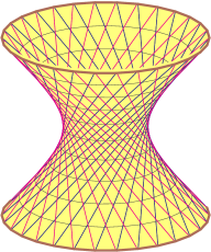
Motivated by [21, § 4], we use fiber products to compute the two rulings of the hyperboloid defined by
Since a generic line meets in two points, a line which meets in three points must be contained in . For each , we associate a line where
Consider the following system on ,
A ruling of corresponds to a four-dimensional irreducible component such that there exists an irreducible curve where
| (7.1) |
In particular, and for .
For , the witness point set consists of isolated points. The following uses our toolkit to determine the irreducible components corresponding to the rulings.
Using Algorithms 2.3 and 2.4, we compute the dimensions of components containing points of under different projections. The following table records the relevant information up to symmetry.
The first column shows that the points of lie on components of having two distinct multidimensions. Let consist of the four points from the first row of this table. For each , the last column implies that the fiber over for distinct is one-dimensional. The trace test shows that each irreducible component of the fiber is linear as expected from (7.1). We note that the number of witness points when treating as system in is and much larger than the number of points in the witness sets in the previous table.
Finally, we compute the irreducible components of . Using monodromy and the trace test in , we partition into two sets of size two, each corresponding to a distinct ruling of the hyperboloid. The rulings correspond to the two irreducible curves
The symbolic expressions of these curves are classically known, but one can also recover them directly from the computed witness points via [1].
7.2. Exceptional planar pentads
A planar pentad is a 3-RR mechanism constructed by connecting the vertices of two triangles by three legs with revolute joints as shown in Figure 4.
We fix one of the triangles in the plane to remove the trivial motion of the entire mechanism. A generic mechanism can be assembled in six different configurations, which is the degree of SE(2) as described in [7, Table 1]. Since a generic planar pentad is rigid (i.e., does not move), a planar pentad is exceptional when it exhibits motion.
Using isotropic coordinates, the parameters in Figure 4 are
with the following assemblability restrictions:
A mechanism is degenerate if a parameter, , , , or is zero. Since nondegenerate mechanisms are desired, we dehomogenize the parameter space by setting . Hence, the parameter space becomes
where
A mechanism is physically meaningful if .
For , the poses corresponding to link lengths satisfy
The six configurations of a general planar pentad correspond with the six points in the witness point set for .
The only family of nondegenerate exceptional planar pentads are the double-parallelogram linkages [22], namely
We aim to compute directly from by using fiber products. Since has codimension four, Corollary 2.14 of [21] shows that will correspond with an irreducible component of the fourth fiber product system, namely
The irreducible component corresponding to is called a main component in [21]. In fact, is a Cartesian product of with four copies of
This corresponds with rotating about a fixed .
A necessary condition for locating such an exceptional component of codimension four consisting of nondegenerate and physically meaningful linkages with one dimension of motion is that there exists such that and . A sufficient condition for such a component to exist is that one of the isolated points in is a general point of . To that end, we first compute the -witness point set for where resulting in 14,828 isolated nonsingular points in . The results of using Algorithm 2.3 to compute the the local dimension at each of these 14,828 witness points along with the local fiber dimensions obtained by fixing the coordinates and coarsening the fiber to the natural are summarized in the following.
The first collection of 14,144 witness points correspond with rigid planar pentads. The second collection of 678 witness points correspond with degenerate planar pentads. The final collection of 6 witness points correspond with five degenerate planar pentads arising from one of the five nonconstant edges of or being zero (recall ). The other witness point in this collection is the unique point in that is a general point on thereby confirming and the existence of nondegenerate exceptional planar pentads. On the other hand, working without the multihomogeneous structure, leads to approximately witness points which we can’t robustly compute.
Acknowledgements
We thank Tim Duff for his helpful comments on the paper.
References
- [1] D.J. Bates, J.D. Hauenstein, T.M. McCoy, C. Peterson, and A.J. Sommese, Recovering exact results from inexact numerical data in algebraic geometry, Experimental Mathematics, 22 (2013), 38–50.
- [2] F. Castillo, B. Li, and N. Zhang, Representable Chow classes of a product of projective spaces, arXiv:1612.00154, 2016.
- [3] T. Duff, C. Hill, A. Jensen, K. Lee, A. Leykin, and J. Sommars, Solving polynomial systems via homotopy continuation and monodromy, IMA Journal of Numerical Analysis 39 (2018), no. 3, 1421–1446.
- [4] W. Fulton, Intersection theory, Ergebnisse der Math., no. 2, Springer-Verlag, 1984.
- [5] J. Harris, Algebraic geometry, Graduate Texts in Mathematics, vol. 133, Springer-Verlag, New York, 1992.
- [6] J.D. Hauenstein and J.I. Rodriguez, Multiprojective witness sets and a trace test, Advances in Geometry, to appear.
- [7] J.D. Hauenstein, S.N. Sherman, and C.W. Wampler, Exceptional Stewart-Gough platforms, Segre embeddings, and the special Euclidean group, SIAM J. Appl. Algebra Geom. 2 (2018), no. 1, 179–205.
- [8] J.D. Hauenstein, A.J. Sommese, and C.W. Wampler, Regeneration homotopies for solving systems of polynomials, Math. Comp. 80 (2011), no. 273, 345–377.
- [9] J.-P. Jouanolou, Théorèmes de Bertini et applications, Progress in Mathematics, vol. 42, Birkhäuser Boston, Inc., Boston, MA, 1983.
- [10] A. Leykin, J.I. Rodriguez, and F. Sottile, Trace test, Arnold Mathematical Journal 4 (2018), no. 1, 113–125.
- [11] E. Miller and B. Sturmfels, Combinatorial commutative algebra, Graduate Texts in Mathematics, vol. 227, Springer-Verlag, New York, 2005.
- [12] A. Morgan, Solving polynomial systems using continuation for engineering and scientific problems, Classics in Applied Mathematics, vol. 57, SIAM, Philadelphia, PA, 2009.
- [13] A. Morgan and A. Sommese, A homotopy for solving general polynomial systems that respects -homogeneous structures, Appl. Math. Comput. 24 (1987), no. 2, 101–113.
- [14] J. Oxley, Matroid theory, second ed., Oxford Graduate Texts in Mathematics, vol. 21, Oxford University Press, Oxford, 2011.
- [15] A. Postnikov, Permutohedra, associahedra, and beyond, Int. Math. Res. Not. IMRN (2009), no. 6, 1026–1106.
- [16] A.J. Sommese and J. Verschelde, Numerical homotopies to compute generic points on positive dimensional algebraic sets, J. Complexity 16 (2000), no. 3, 572–602.
- [17] A.J. Sommese, J. Verschelde, and C.W. Wampler, Numerical decomposition of the solution sets of polynomial systems into irreducible components, SIAM J. Numer. Anal. 38 (2001), no. 6, 2022–2046.
- [18] by same author, Using monodromy to decompose solution sets of polynomial systems into irreducible components, Applications of algebraic geometry to coding theory, physics and computation (Eilat, 2001), NATO Sci. Ser. II Math. Phys. Chem., vol. 36, Kluwer Acad. Publ., Dordrecht, 2001, pp. 297–315.
- [19] by same author, Symmetric functions applied to decomposing solution sets of polynomial systems, SIAM J. Numer. Anal. 40 (2002), no. 6, 2026–2046.
- [20] A.J. Sommese and C.W. Wampler, The numerical solution of systems of polynomials, World Scientific Publishing Co. Pte. Ltd., Hackensack, NJ, 2005.
- [21] by same author, Exceptional sets and fiber products, Found. Comput. Math. 8 (2008), no. 2, 171–196.
- [22] C.W. Wampler and A.J. Sommese, Numerical algebraic geometry and algebraic kinematics, Acta Numer. 20 (2011), 469–567.