Fluctuation dynamics of an open photon Bose-Einstein condensate

Abstract

Bosonic gases coupled to a particle reservoir have proven to support a regime of operation where Bose-Einstein condensation coexists with unusually large particle-number fluctuations. Experimentally, this situation has been realized with two-dimensional photon gases in a dye-filled optical microcavity. Here, we investigate theoretically and experimentally the open-system dynamics of a grand canonical Bose-Einstein condensate of photons. We identify a regime with temporal oscillations of the second-order coherence function $g^{(2)}(\tau)$, even though the energy spectrum closely matches the predictions for an equilibrium Bose-Einstein distribution and the system is operated deeply in the regime of weak light-matter coupling. The observed temporal oscillations are attributed to the nonlinear, weakly driven-dissipative nature of the system which leads to time-reversal symmetry breaking.

I Introduction

Bose-Einstein condensates are the experimental basis of a variety of observed collective quantum phenomena Pitaevskiĭ and Stringari (2003); Bloch et al. (2008). Generally, Bose-Einstein condensation is a phenomenon in thermodynamic equilibrium for Bose systems, usually described for a fixed total particle number, which leads to a macroscopic ground-state occupation. In ultracold atomic gases Anderson et al. (1995); Davis et al. (1995) and exciton-polariton systems Kasprzak et al. (2006); Balili et al. (2007), condensation has been observed following thermalization by interparticle collisions, a process that leaves the total particle number constant. Photons usually do not exhibit condensation, with the chemical potential vanishing at all temperatures in the well-known example of a (three-dimensional) blackbody radiator. Two-dimensional photon gases under harmonic confinement can, however, reach condensation, as was experimentally demonstrated in dye-filled optical microcavities Klaers et al. (2010); Marelic and Nyman (2015); Greveling et al. (2018). In this system, thermalization is reached by absorption and re-emission processes on the dye molecules, which leaves the average particle number constant but allows for fluctuations around this average value. In the limit of number fluctuations that become as large as the average particle number, such a situation is described well by the grand canonical statistical ensemble Fujiwara et al. (1970); Ziff et al. (1977); Klaers et al. (2012); Sob’yanin (2012). Lasers are long-known physical systems that also have macroscopic population of excited states, but which operate far from thermal equilibrium Zamora et al. (2017); Vorberg et al. (2018). The crossover from lasing to condensation, characterized by a varying degree of thermalization, has been investigated by observing deviations from a thermalized distribution, both in polariton and photon gases Deng et al. (2010); Byrnes et al. (2014); Sun et al. (2017); Kirton and Keeling (2013); Schmitt et al. (2015); Marelic and Nyman (2015). Particle-number conserving condensates as well as lasers are characterized by vanishing particle-number fluctuations in the thermodynamic limit, i.e., by a value of the second-order coherence function of $g^{(2)}(\tau)=1$ at all delay times $\tau$.

Experimentally, evidence for Bose-Einstein condensation in the grand canonical statistical regime with unusually large statistical number fluctuations has been observed with photons in the dye microcavity system Schmitt et al. (2014). The coupling of photons to the photo-excitable dye molecules implies that the dye does not only act as a heat bath, but also as a particle reservoir due to the possible interconversion of photons and dye electronic excitations. For a large relative size of the dye reservoir, this leads to strikingly enhanced statistical number fluctuations and a zero-delay second-order correlation $g^{(2)}(0)=2$, i.e., as in a thermal source. Notably, these fluctuations, which can be as large as the average value, occur deep in the condensed phase. On the other hand, with a smaller effective relative size of the dye reservoir, the dye microcavity photon condensate can also be operated in the (usual) canonical statistical regime, with much smaller number fluctuations and a zero-delay intensity correlation $g^{(2)}(0)=1$. Independent of the ensemble conditions, frequent collisions of solvent molecules with the dye on a timescale of $10^{-14}$ s Lakowicz (2006), cause the dye microcavity condensate to operate in the weakly coupled regime of matter and light Angelis et al. (2000); Yokoyama and Brorson (1989), i.e., the trapped particles are photons (not polaritons) and the system can be well described by a rate equation model, with, e.g., no Rabi oscillations occurring.

In the present work, we examine the temporal dynamics of a photon Bose-Einstein condensate (BEC) in the strongly fluctuating regime, where a steady driven-dissipative state is induced by a balance of continuous dye pumping and cavity losses. We observe distinct temporal oscillations of the photon number correlations $g^{(2)}(\tau)$, even though the spectral photon distribution is, within experimental uncertainties, indistinguishable from predictions for thermodynamic equilibrium (Bose-Einstein distribution). Temporal oscillations of density fluctuations have been observed, e.g. in oscillatory relaxation dynamics in lasers Takemura et al. (2012) and in driven-dissipative atomic Bose-Einstein condensates confined in high-finesse optical cavities Brennecke et al. (2013). Damped, oscillatory displacement dynamics have been observed in colloids suspended in liquids upon driving out of equilibrium Berner et al. (2018), see also theoretical work proposing corresponding experiments with laser-driven quantum dots Moradi et al. (2018). In all those systems, however, the (temporally averaged) spectrum clearly differs from the thermodynamic equilibrium distribution.

For the correlation dynamics of the photon BEC, we find quantitative agreement with a theoretical analysis in terms of nonlinear rate equations. We are thus able to trace back the origin of the correlation oscillations to the coupling of the dye reservoir and the condensate photons, combined with time-reversal symmetry breaking in the (weakly) driven-dissipative state. The nonlinearity of the coupling implies that the dynamics of $g^{(2)}(\tau)$ will depend on the steady state of the system.

The paper is organized as follows. Section II provides some details of the experimental setup and mode of operation. In Section III we derive the rate equations for the nonequilibrium dynamics of the average numbers of photons and of dye-molecule excitations as well as for the autocorrelation functions of these quantities. In Section IV we present and discuss the experimental results, along with the comparison to the theory. We conclude in Section V with an outlook to further studies.

II Experimental setup and mode of operation

Our experimental setup for trapping a two-dimensional photon gas in a dye-filled optical microcavity is similar to that described in earlier work Klaers et al. (2010, 2011), as shown in Fig. 1. The cavity is composed of two highly reflecting mirrors (reflectivity $>99.998\%$) of $1$ m curvature radius spaced by $\approx 2\leavevmode\nobreak\ \upmu$m distance, and is filled with rhodamine dye dissolved in ethylene glycol ($1$ mmol/L). Due to the small mirror spacing, the cavity has a longitudinal mode spacing comparable to the emission width of the dye. In this regime, we observe that only photons of a fixed longitudinal mode number $q$ populate the cavity, with $q=7$ in our setup. This imposes an upper limit on the optical wavelength and a restriction of energies to a minimum cutoff of $\hbar\omega_{c}\approx 2.1$ eV for photons in the cavity, where $\omega_{c}$ is the cutoff frequency of the cavity with transverse momentum $k_{r}=0$. The optical dispersion becomes quadratic and the mirror curvature induces a trapping potential for the photons (see Fig. 1). One can show that the system is formally equivalent to a harmonically trapped two-dimensional gas of massive particles for which – other than for (three-dimensional) blackbody radiation – Bose-Einstein condensation is possible for a thermalized ensemble Klaers et al. (2010). To initially populate the cavity and compensate for losses from e.g., mirror transmission, the dye is pumped to a stationary state with an external laser beam.

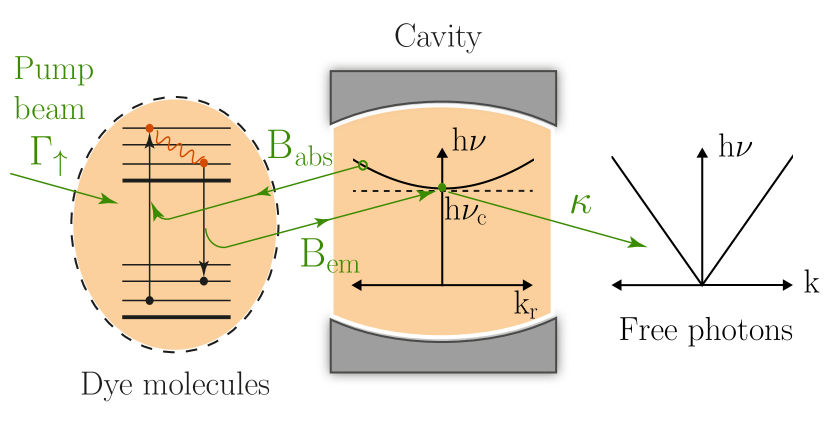
Figure 1: The photon flow through the condensed photon gas in the dye-filled microcavity. The dye molecules, which are excited with a pump rate $\Gamma_{\uparrow}$ constitute a heat and particle reservoir for the condensed photons. The photon dispersion in the cavity in terms of the transverse wave vector is $h\nu=\sqrt{(h\nu_{c})^{2}+(\hbar ck_{r})^{2}}$, with $\nu_{c}=\omega_{c}/2\pi$ the cavity cutoff frequency and $c$ the light velocity in the dye medium. The photon loss rate of the condensate through the cavity mirrors is represented by $\kappa$.

To record the statistics as well as the number correlations of the photon condensate, the microcavity emission is directed through an optical telescope and a mode filter consisting of a $10.6$ mm diameter iris to separate the condensate mode from the higher-mode (thermal cloud) photons. Even though the divergence of the higher-order modes is larger than that of the ground mode, they contribute residually to the intensity near the optical axis in the far field, and a fraction of photons in these modes is consequently transmitted through the momentum filter. This imperfection of the mode filtering reduces the magnitude of the measured (normalized) intensity correlations. As a result, the measured correlations are smaller than the calculated values for the respective system parameters. We do not expect the temporal shape of the correlation signal to be affected by the imperfect mode filtering.

The light passing through the momentum filter is then sent through a polarizer to remove the polarization degeneracy and then imaged onto a fast ($5$ GHz bandwidth) photomultiplier. The electronic output signal of the photomultiplier is analyzed employing a $3.5$ GHz bandwidth oscilloscope. To suppress the influence of electronic noise of the high-bandwidth electronic analysis system (which is mainly attributed to the oscilloscope’s analog-digital converters), the photomultiplier output is simultaneously recorded by two oscilloscope channels, with the cross-correlation used for further data analysis of the fluctuations. Calibration of the photomultiplier signal is performed via the measured spectra, which relate the photon number in the condensate peak to the known critical photon number in the thermal photon cloud of $N_{c}=\pi^{2}/3(k_{B}T/\hbar\Omega)^{2}=80660$ for the used experimental parameters ($T=300$ K, trap frequency $\Omega=2\pi\cdot 40$ GHz).

The dephasing time $\tau_{\varphi}$ of dye excitations (given by the collision time of solvent molecules with the dye on a scale of $10^{-14}$ s is much shorter than the photon lifetime in the cavity ($\tau_{\mathrm{p}}\approx 0.5$ ns, determined by cavity losses), $\tau_{\varphi}\ll\tau_{\mathrm{p}}$. Furthermore, coherence between dye excitations and photons cannot be established, that is, our experiment operates in the weakly coupled regime of matter and light, and the trapped particles are photons, not polaritons Angelis et al. (2000); Yokoyama and Brorson (1989)). The photon lifetime, in turn, is much shorter than the nonradiative decay time of dye excitations, $\tau_{\mathrm{p}}\ll\tau_{\mathrm{nrad}}$ (with $\tau_{\mathrm{nrad}}$ being in the order of 50 ns Barroso et al. (1998). This means that the sum of the number of cavity photons (including the thermal mode photons) and the dye excitation number can be considered conserved on the time scale of the photon lifetime $\tau_{\mathrm{p}}$, where the photon number alone is fixed on average only. To good approximation, also the sum of the number of condensate mode photons and dye excitations is conserved, as exchange between thermal cloud photons and condensate mode photons only occurs via the bath and the dye excitation number exceeds the (thermal mode) photon number by many orders of magnitude Klaers et al. (2012) For sufficiently fast energy exchange with the dye reservoir, i.e., if several absorption and re-emission cycles occur before a photon is lost, the photons reach a thermal spectral distribution at the rovibrational temperature of the dye, which is at room temperature ($300$ K). Fig. 2 shows measurements of the optical spectrum for different average condensate photon numbers $\langle n\rangle_{\infty}$ (different pump rates). The visible good agreement of the the experimental data (dots) with the predictions of equilibrium theory (solid lines) confirms that in our experiments, a thermal distribution is achieved to good approximation, despite continuous pumping and losses. Above a critical photon number, the thermal photon gas eventually forms a BEC, signaled by the condensate peak in the spectral distribution at the position of the low-frequency cavity cutoff on top of a broad thermal photon cloud Klaers et al. (2010).

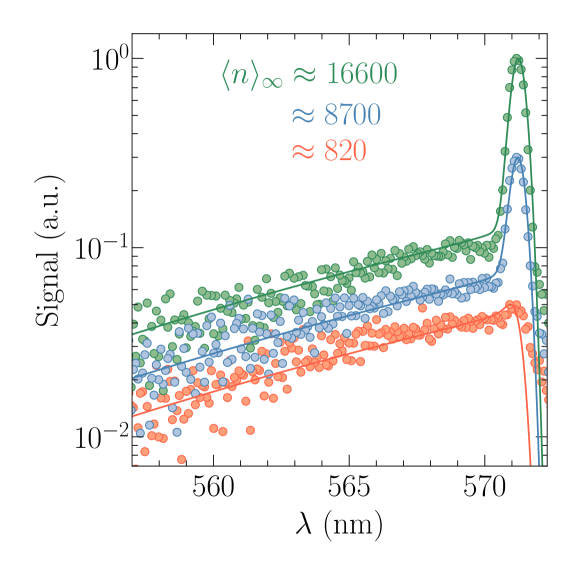
Figure 2: Optical spectra (arbitrary units) as a function of wavelength $\lambda$, taken from cavity emission through the mirrors at the cutoff wavelength of $\lambda_{c}=571.3$ nm, where the experiment was conducted. The solid lines are fits of the Bose-Einstein distribution at $300$K (broadened by the experimental resolution) to the experimental data, with the steady-state average condensate photon number $\langle n\rangle_{\infty}$ as the only adjustable parameter. The fitted values of $\langle n\rangle_{\infty}$ are shown in the legend. The spectra at different $\langle n\rangle_{\infty}$ are vertically shifted for clarity.

By varying the photon number $\langle n\rangle_{\infty}$ with respect to the number of dye reservoir molecules $M$ within the cavity volume, the photon number statistics can be continuously tuned from a small relative reservoir size with Poissonian statistics and $g^{(2)}(0)\approx 1$ to a strongly fluctuating state of small relative photon number with Bose-Einstein statistics and $g^{(2)}(0)\approx 2$ Schmitt et al. (2014).

III Theoretical description

III.1 Model and master equation

The thermalization dynamics of the dye-filled microcavity has been studied Kirton and Keeling (2013, 2015); Keeling and Kirton (2016) employing a Frank-Condon model for the dye molecules: The two-level system of the electronic ground and excited states, between which the optical transitions occur, is coupled to a molecular vibrational degree of freedom (phonon) because the rest position of the ionic molecular oscillator depends on whether the molecule is in its electronic ground or excited state. The total number of dye molecules is $M=M_{\uparrow}+M_{\downarrow}$, where $M_{\uparrow}$ and $M_{\downarrow}$ are the number of molecules in the electronically excited or ground state, respectively. The Hamiltonian for the dye-filled microcavity reads thus Marthaler et al. (2011)

$$\begin{split}H&=\sum_{k}\omega_{k}^{\phantom{\dagger}}a^{\dagger}_{k}a^{\phantom{\dagger}}_{k}+\sum_{m=1}^{M}\left[\frac{\delta}{2}\sigma^{z}_{m}+\Omega\,b^{\dagger}_{m}b_{m}\right.\\ &+\left.\Omega\sqrt{S}\,\sigma^{z}_{m}\left(b_{m}+b^{\dagger}_{m}\right)+g\sum_{k}\left(a^{\phantom{\dagger}}_{k}\sigma^{+}_{m}+a^{\dagger}_{k}\sigma^{-}_{m}\right)\right],\end{split}$$ (1)

in units such that $\hbar=1$. The cavity-photon modes with transverse dispersion $\omega_{k}$ are represented by the bosonic operators $a_{k}$, $a^{\dagger}_{k}$, the vibronic states of dye molecule $m$ with oscillator frequency $\Omega$ by $b_{m}$, $b^{\dagger}_{m}$, and the electronic two-level system of molecule $m$ by the Pauli matrix $\sigma^{z}_{m}$ and and raising/lowering operators $\sigma^{\pm}_{m}$, with the electronic transition frequency $\delta$. The Frank-Condon electron-phonon coupling is parametrized by $S$, where the phonon position operator is $\hat{x}\propto\left(b_{m}+b^{\dagger}_{m}\right)$. The last term in Eq. (1) describes photon emission or absorption with the optical transition matrix element $g$, the smallest energy scale in the system. Since we consider photon gases which have already reached a stationary, thermal distribution, and since in the experiment the transverse cavity ground-state mode (condensate mode) is singled out, the analysis may be restricted to the photon correlations in the condensate, i.e., we will collapse the sum over cavity modes in Eq. (1) to $k=0$, where $\omega_{c}\equiv\omega_{0}$ is the cavity-cutoff frequency (see also Fig. 1). The cutoff is chosen such that the cavity detuning is $\Delta=\omega_{c}-\delta<0$. From here on, we will drop the cavity-mode subscript on the photon operators and write $a\equiv a_{0}$.

The molecular part of the Hamiltonian can be diagonalized by a polaron transformation Marthaler et al. (2011). This leads to an effective, nonlinear electron-photon coupling, mediated by the phonon excitations of the dye. Due to fast collisions of the dye molecules with solvent molecules, the phonon excitations may be considered to be in thermal equilibrium at ambient temperature. After treating the phonon excitations as a Markovian thermal bath, this coupling can be parametrized by a coherent part $g_{\beta}$ Radonjić et al. (2018), and incoherent, phonon-assisted couplings $B_{\text{abs}}$ for photon absorption and $B_{\text{em}}$ for photon emission (see Fig. 1). For the density matrix $\rho$, one obtains in this way the master equation

$$\begin{split}\dot{\rho}=\mathrm{i}\,[\rho,H_{0}]+\kappa\mathcal{L}[a]\rho+\sum_{m=1}^{M}\mathcal{L}_{m}\rho,\end{split}$$ (2)

where $H_{0}=\Delta a^{\dagger}a+\sum_{m=1}^{M}g_{\beta}\left(a^{\dagger}\sigma_{m}^{-}+a\sigma_{m}^{+}\right)$ is the Hamiltonian generating the coherent part of the evolution in the rotated frame. The parameter $\kappa$ in Eq. (2) describes the cavity loss to the environment, where the Lindblad operator acting on the density matrix $\rho$ is defined as $\mathcal{L}[X]\rho=\tfrac{1}{2}\left([X\rho,X^{\dagger}]+[X,\rho X^{\dagger}]\right)$. The molecule-induced superoperator $\mathcal{L}_{m}$ is given by

$$\mathcal{L}_{m}=\Gamma_{\uparrow}\mathcal{L}[\sigma^{+}_{m}]+\Gamma_{\downarrow}\mathcal{L}[\sigma^{-}_{m}]+B_{\text{abs}}\mathcal{L}[a\sigma^{+}_{m}]+B_{\text{em}}\mathcal{L}[a^{\dagger}\sigma^{-}_{m}].$$ (3)

The four terms in $\mathcal{L}_{m}$ describe, in order of appearance, pumping by an external laser source ($\Gamma_{\uparrow}$), nonradiative decay of dye excitations ($\Gamma_{\downarrow}\ll\Gamma_{\uparrow}$), and photon absorption ($B_{\text{abs}}$) and emission ($B_{\text{em}}$) by the dye molecules, respectively.

Since the experiment operates in the regime $g_{\beta}/g\ll 1$ Radonjić et al. (2018), and the detuning is very large compared to the renormalized coherent coupling, $|\Delta|\gg g_{\beta}$, the cavity mode effectively couples to the molecules only incoherently via the Lindblad terms proportional to $B_{\text{abs}}$ or $B_{\text{em}}$. Therefore, the contribution of $H_{0}$ to the master equation (2) can be neglected for the present setup Kirton and Keeling (2013). In addition, one should note that $B_{\text{em}}>B_{\text{abs}}$ because of the red detuning of the cavity cutoff $\omega_{c}$ with respect to the electronic dye excitation energy $\delta$.

III.2 Average particle numbers

The coupled rate equations for the average condensate mode photon number $\langle n\rangle$ and the number of dye molecules in excited states $\langle M_{\uparrow}\rangle$ can now be derived from the master equation, where $\langle\cdot\rangle=\mathrm{Tr}[\rho(t)\cdot]$ denotes the thermal and quantum mechanical average. Inserting $\dot{\rho}$ from Eqs. (2) and (3), using cyclic permutation under the trace, and $\sigma_{m}^{\pm}\sigma_{m}^{\mp}=(1\pm\sigma_{m}^{z})/2$, leads to operator products of $M_{\uparrow}=\sum_{m}(1+\sigma_{m}^{z})/2$ and $n=a^{\dagger}a$. Again because of the fast dye-solvent collisions, coherent propagation of excitations of different dye molecules ($m^{\prime}\neq m$) is negligible. This means that the sum over a large number of molecules amounts to an average, $\langle M_{\uparrow}\rangle=\sum_{m}(1+\langle\sigma_{m}^{z}\rangle)/2=M(1+\langle\sigma_{m}^{z}\rangle)/2$, and expectation values of higher-order operator products factorize, $\langle nM_{\uparrow}\rangle\approx\langle n\rangle\langle M_{\uparrow}\rangle$. In this way, one obtains the nonlinear, coupled rate equations

$$\begin{split}\frac{\mathrm{d}}{\mathrm{d}t}{\langle n\rangle}&=-\kappa\langle n\rangle-B_{\text{abs}}\left(M-\langle M_{\uparrow}\rangle\right)\langle n\rangle\\ &+B_{\text{em}}\left(\langle n\rangle+1\right)\langle M_{\uparrow}\rangle,\end{split}$$ (4a)

$$\begin{split}\frac{\mathrm{d}}{\mathrm{d}t}{\langle M_{\uparrow}\rangle}&=\Gamma_{\uparrow}\left(M-\langle M_{\uparrow}\rangle\right)-\Gamma_{\downarrow}\langle M_{\uparrow}\rangle\\ &+B_{\text{abs}}\left(M-\langle M_{\uparrow}\rangle\right)\langle n\rangle-B_{\text{em}}\left(\langle n\rangle+1\right)\langle M_{\uparrow}\rangle.\end{split}$$ (4b)

These agree, in fact, with the semiclassical rate equations expected phenomenologically from pumping and nonradiative decay of molecule excitations a well as stimulated and spontaneous photon emission into the cavity. Alternatively, one may solve the untruncated rate equations for $\langle n\rangle$ and $\langle M_{\uparrow}\rangle$ together with three equations for the second moments Kirton and Keeling (2015). This is discussed in detail in the Appendix. For large $M$, both solution methods give the same results for $\langle n\rangle$ and $\langle M_{\uparrow}\rangle$ in the long-time limit.

To calculate the steady-state second-order photon correlations in the next section, it will be necessary to have the average numbers of photons and excited molecules in the steady state which is reached in the long-time limit, $\langle n\rangle_{\infty}$ and $\langle M_{\uparrow}\rangle_{\infty}$. This amounts to setting the time derivatives in Eqs. (4) to zero, and one obtains for large molecule number $M\gg 1$,

$$\langle n\rangle_{\infty} =\frac{M\left(B_{\text{em}}\Gamma_{\uparrow}-B_{\text{abs}}\Gamma_{\downarrow}\right)}{\kappa\left(B_{\text{em}}+B_{\text{abs}}\right)}+\mathcal{O}(1),$$ (5)

$$\langle M_{\uparrow}\rangle_{\infty} =\frac{MB_{\text{abs}}+\kappa}{B_{\text{abs}}+B_{\text{em}}}+\mathcal{O}(1/M).$$ (6)

In our experiments, the pump rate strongly exceeds the nonradiative decay, $\Gamma_{\uparrow}\gg\Gamma_{\downarrow}$, and $B_{\text{em}}+B_{\text{abs}}\approx B_{\text{em}}$. The ratio of emission and absorption is given by $B_{\text{em}}/B_{\text{abs}}=\exp(-\hbar\Delta/k_{B}T)$, where $T$ is the phonon temperature (Kennard-Stepanov relation). With these simplifications, the steady-state photon number becomes approximately

$$\langle n\rangle_{\infty}\approx\frac{M\Gamma_{\uparrow}}{\kappa}.$$ (7)

This expression is useful for converting $\langle n\rangle_{\infty}$, which is measured in the experiments, into the pump parameter $\Gamma_{\uparrow}$ of the theoretical model and vice versa. When comparing to experimental data, however, a full numerical solution for the steady state of Eqs. (4) and (25) is used.

III.3 Second-order correlation function

The time-dependent photon density-density or second-order correlation function measured in the experiment is defined as

$$\begin{split}g^{(2)}(\tau)&=\left.\frac{\langle n(t+\tau)n(t)\rangle}{\langle n(t)\rangle^{2}}\right|_{t\to\infty}=\frac{\mathrm{Tr}\left[a^{\dagger}a\;\mathrm{e}^{\hat{L}\tau}\tilde{\rho}_{\infty}\right]}{\mathrm{Tr}\left[a^{\dagger}a\rho_{\infty}\right]^{2}},\end{split}$$ (8)

where $\hat{L}$ is the total Liouvillian superoperator belonging to the master equation (2), $\rho_{\infty}=\lim_{t\to\infty}\rho(t)$ denotes the steady-state density matrix, and we define $\tilde{\rho}_{\infty}:=a^{\dagger}a\rho_{\infty}$. Note in passing that, for the normal-ordered second-order correlation function, one would need to set $\tilde{\rho}_{\infty}=a\rho_{\infty}a^{\dagger}$. Defining also an effective average $\overline{X}:=\mathrm{Tr}X\mathrm{e}^{\hat{L}\tau}\tilde{\rho}_{\infty}$, one has $g^{(2)}(\tau)=\overline{n}/\langle n\rangle_{\infty}^{2}$. Formally, $\overline{n}$ and $\overline{M}_{\uparrow}$ obey almost the same definitions as $\langle n\rangle$ and $\langle M_{\uparrow}\rangle$, however with $\rho(t)$ replaced by $\mathrm{e}^{\hat{L}\tau}\tilde{\rho}_{\infty}$ and $\mathrm{Tr}\,\tilde{\rho}_{\infty}=\langle n\rangle_{\infty}$. Thus, one finds equations of motion analogous to Eqs. (4a) and (4b),

$$\begin{split}\frac{\mathrm{d}}{\mathrm{d}\tau}\overline{n}&=-\kappa\overline{n}-B_{\text{abs}}\overline{(M-M_{\uparrow})n}\\ &+B_{\text{em}}\overline{(n+1)M_{\uparrow}},\end{split}$$ (9a)

$$\begin{split}\frac{\mathrm{d}}{\mathrm{d}\tau}\overline{M_{\uparrow}}&=\Gamma_{\uparrow}\left(\langle n\rangle_{\infty}M-\overline{M_{\uparrow}}\right)-\Gamma_{\downarrow}\overline{M_{\uparrow}}\\ &+B_{\text{abs}}\overline{(M-M_{\uparrow})n}-B_{\text{em}}\overline{(n+1)M_{\uparrow}}.\end{split}$$ (9b)

The cluster expansions of averages of the higher-order operator products $\overline{nM_{\uparrow}}$ are truncated under the same conditions as discussed in the previous section (incoherent propagation of excitations of different molecules). This amounts to letting $\overline{nM_{\uparrow}}=\langle n\rangle_{\infty}\overline{M_{\uparrow}}+\langle n\rangle_{\infty}\langle nM_{\uparrow}\rangle_{\infty}+\langle M_{\uparrow}\rangle_{\infty}\overline{n}-2\langle n\rangle_{\infty}^{2}\langle M_{\uparrow}\rangle_{\infty}$. By computing the steady-state density matrix numerically exactly for different molecule numbers of order $M\sim 10^{2}$, we have checked that the truncation is well justified already for intermediate system sizes, i.e. above threshold Kirton and Keeling (2015). The experiment is operated far inside this range of validity. Above threshold, we also have $\Gamma_{\uparrow}\gg\Gamma_{\downarrow}$, such that we may safely neglect the non-radiative molecule decay rate $\Gamma_{\downarrow}$ for the evaluations in Section IV.

In terms of the deviations of the second-order correlation functions from their relaxed values (attained for $\tau\to\infty$),

$$\boldsymbol{g}=\begin{pmatrix}\Delta g^{(2)}_{n}\\ \Delta g^{(2)}_{n,\,M_{\uparrow}}\end{pmatrix}=\begin{pmatrix}\overline{n}-\langle n\rangle_{\infty}^{2}\\ \overline{M}_{\uparrow}-\langle n\rangle_{\infty}\langle M_{\uparrow}\rangle_{\infty}\end{pmatrix},$$ (10)

Eqs. (9) then become

$$\begin{split}\frac{\mathrm{d}}{\mathrm{d}\tau}\Delta g_{n}^{(2)}&=\langle n\rangle_{\infty}\Big{[}-\kappa\langle n\rangle_{\infty}-B_{\text{abs}}\left(M-\langle M_{\uparrow}\rangle_{\infty}\right)\langle n\rangle_{\infty}\\ &+B_{\text{em}}\left(\langle n\rangle_{\infty}+1\right)\langle M_{\uparrow}\rangle_{\infty}\Big{]}-\kappa\Delta g_{n}^{(2)}\\ &-B_{\text{abs}}\left[(M-\langle M_{\uparrow}\rangle_{\infty})\Delta g_{n}^{(2)}-\langle n\rangle_{\infty}\Delta g_{n,\,M_{\uparrow}}^{(2)}\right]\\ &+B_{\text{em}}\left[(\langle n\rangle_{\infty}+1)\Delta g_{n,\,M_{\uparrow}}^{(2)}+\langle M_{\uparrow}\rangle_{\infty}\Delta g_{n}^{(2)}\right],\end{split}$$ (11a)

$$\begin{split}\frac{\mathrm{d}}{\mathrm{d}\tau}\Delta g_{n,\,M_{\uparrow}}^{(2)}&=\langle n\rangle_{\infty}\Big{[}\Gamma_{\uparrow}\left(M-\langle M_{\uparrow}\rangle_{\infty}\right)-\Gamma_{\downarrow}\langle M_{\uparrow}\rangle_{\infty}\\ &+B_{\text{abs}}\left(M-\langle M_{\uparrow}\rangle_{\infty}\right)\langle n\rangle_{\infty}\\ &-B_{\text{em}}\left(\langle n\rangle_{\infty}+1\right)\langle M_{\uparrow}\rangle_{\infty}\Big{]}-(\Gamma_{\uparrow}+\Gamma_{\downarrow})\Delta g_{n,\,M_{\uparrow}}^{(2)}\\ &+B_{\text{abs}}\left[(M-\langle M_{\uparrow}\rangle_{\infty})\Delta g_{n}^{(2)}-\langle n\rangle_{\infty}\Delta g_{n,\,M_{\uparrow}}^{(2)}\right]\\ &-B_{\text{em}}\left[(\langle n\rangle_{\infty}+1)\Delta g_{n,\,M_{\uparrow}}^{(2)}+\langle M_{\uparrow}\rangle_{\infty}\Delta g_{n}^{(2)}\right].\end{split}$$ (11b)

Using the steady-state solution of Eqs. (4), one eventually finds a system of two coupled linear equations,

$$\partial_{\tau}\boldsymbol{g}=\begin{pmatrix}-\kappa-\tilde{\Gamma}_{M}&\tilde{\Gamma}_{n}\\ \tilde{\Gamma}_{M}&-\left(\Gamma_{\uparrow}+\Gamma_{\downarrow}\right)-\tilde{\Gamma}_{n}\end{pmatrix}\boldsymbol{g}.$$ (12)

The matrix elements are given by

$$\begin{split}\tilde{\Gamma}_{M}&=B_{\text{abs}}(M-\langle M_{\uparrow}\rangle_{\infty})-B_{\text{em}}\langle M_{\uparrow}\rangle_{\infty},\\ \tilde{\Gamma}_{n}&=B_{\text{abs}}\langle n\rangle_{\infty}+B_{\text{em}}(\langle n\rangle_{\infty}+1).\end{split}$$ (13)

The coupling constant $\tilde{\Gamma}_{M}$ is composed of an absorption term proportional to the number of ground-state molecules in the steady state ($M-\langle M_{\uparrow}\rangle_{\infty}$), and a corresponding emission term with the number of excited molecules. The coupling constant $\tilde{\Gamma}_{n}$ is given by an absorption term, and the terms corresponding to stimulated and spontaneous emission.

The result of Eq. (12) is equivalent to what one would obtain from linearizing Eqs. (4) around the steady state and then applying the regression theorem.

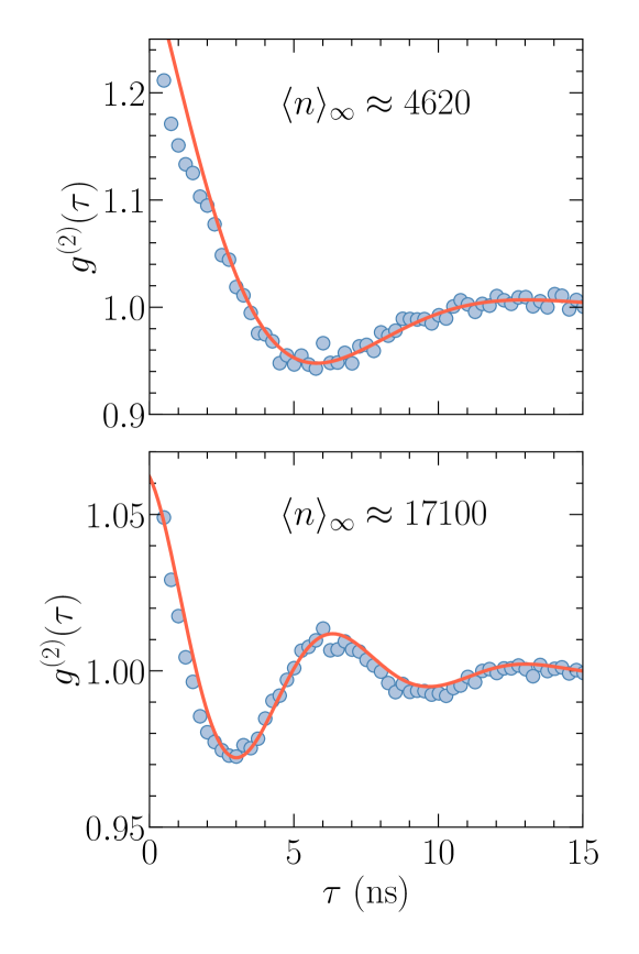
Figure 3: Typical results for the time dependence of the second-order correlation function for two different photon numbers in the condensate, as indicated. The solid lines are fits to the model function, Eq. (19). The envelope of the observed correlation signal $g^{(2)}(\tau)$ temporally decays with a typical relaxation time of about 4 ns.

IV Results

The coupling matrix in Eq. (12) is non-Hermitian because of time-reversal symmetry breaking in the driven-dissipative system. As a result, its eigenvalues are found to be complex, $\lambda=\lambda^{\prime}\pm\mathrm{i}\,\lambda^{\prime\prime}$, where $\lambda^{\prime},\lambda^{\prime\prime}\in\mathds{R}$. In terms of the quantities defined in Eqs. (13), the eigenvalues are given by

$$\begin{split}\lambda&=-\gamma\pm\sqrt{\gamma^{2}-\omega_{0}^{2}},\end{split}$$ (14)

where

$$2\gamma =\kappa+\Gamma_{\uparrow}+\Gamma_{\downarrow}+\tilde{\Gamma}_{M}+\tilde{\Gamma}_{n},$$ (15a)

$$\omega_{0}^{2} =\kappa\tilde{\Gamma}_{n}+(\kappa+\tilde{\Gamma}_{M})(\Gamma_{\uparrow}+\Gamma_{\downarrow}).$$ (15b)

For $\Gamma_{\downarrow}=0$, $B_{\text{abs}}=\alpha B_{\text{em}}$ and to leading order in $1/M$, this reduces to more insightful approximate expressions. In this case, we have

$$\langle n\rangle_{\infty} \approx M\frac{\Gamma_{\uparrow}}{(1+\alpha)\kappa},$$ (16a)

$$\langle M_{\uparrow}\rangle_{\infty} \approx\frac{M\alpha B_{\text{em}}+\kappa}{(1+\alpha)B_{\text{em}}}.$$ (16b)

This gives $\tilde{\Gamma}_{M}=-\kappa$ and $\tilde{\Gamma}_{n}=M\Gamma_{\uparrow}B_{\text{em}}/\kappa$, from which we find

$$\gamma =\frac{\Gamma_{\uparrow}}{2}\left(1+\frac{MB_{\text{em}}}{\kappa}\right)\approx\frac{M\Gamma_{\uparrow}B_{\text{em}}}{2\kappa},$$ (17a)

$$\omega_{0}^{2} =M\Gamma_{\uparrow}B_{\text{em}}.$$ (17b)

Hence, the eigenvalues are given by

$$\begin{split}\lambda&=-\frac{M\Gamma_{\uparrow}B_{\text{em}}}{2\kappa}\pm\frac{1}{2}\sqrt{\left(\frac{M\Gamma_{\uparrow}B_{\text{em}}}{\kappa}\right)^{2}-4M\Gamma_{\uparrow}B_{\text{em}}}.\end{split}$$ (18)

Without drive and dissipation ($\Gamma_{\uparrow}=\kappa=0$), we have a two-component system which shows a single relaxation time, i.e. the system possesses one zero eigenvalue and a purely real eigenvalue $\lambda=-(\tilde{\Gamma}_{M}+\tilde{\Gamma}_{n})$. Correspondingly, the open-system character here is necessary to achieve an imaginary part for the eigenvalues and hence an oscillating photon-number correlation.

Note that this approximation leading to Eq. (18) is not employed in the analysis of the experimental data. It rather serves to illustrate how the openness of the system influences the eigenvalues through the steady-state occupations by making the dependence on $\Gamma_{\uparrow}$ and $\kappa$ explicit.

For the second-order correlation function, one hence finds a solution of the form

$$g^{(2)}_{n}(\tau)=1+\mathrm{e}^{\lambda^{\prime}\tau}\left[c_{1}\cos({\lambda^{\prime\prime}\,\tau})+c_{2}\sin({\lambda^{\prime\prime}\,\tau})\right],$$ (19)

with the real part $\lambda^{\prime}<0$. The initial values for the dynamics of the second-order correlation functions are found from the steady-state solutions for the second moments, $\langle n^{2}\rangle_{\infty}$ and $\langle nM_{\uparrow}\rangle_{\infty}$. Typical experimental data for the temporal variation of the second-order coherence function are given in Fig. 3 for average photon numbers $\langle n\rangle_{\infty}\approx 4620$ and $\langle n\rangle_{\infty}\approx 17100$, respectively, showing damped, oscillatory behavior, as expected from the theoretical analysis. Within the studied experimental parameters, the oscillations persist as the system is tuned between grand canonical and canonical statistical regimes. As can be seen in the two examples of Fig. 3, the magnitude of photon number fluctuations (relative to the average photon number) decreases at higher average photon numbers corresponding to a smaller relative size of the dye reservoir. This behavior has been studied in more detail in earlier work Schmitt et al. (2014). For the present system, the theoretical values for $g^{(2)}(0)$ of the condensate mode at $\langle n\rangle_{\infty}\approx 4620$ and $\langle n\rangle_{\infty}\approx 17100$ are $\approx 2$ and $\approx 1.3$, respectively. As described above, the smaller $g^{(2)}(0)$ values observed in the experimental system are attributed to imperfect mode filtering, which tends to reduce the magnitude of the correlation signal towards that of an uncorrelated sample, where $g^{(2)}(\tau)=1$ for all times $\tau$. The solid lines in Fig. 3 are fits of the function from Eq. (19) to the experimental data, with the imperfect mode filtering resulting in a lowering of the coefficients $c_{1}$,$c_{2}$ with respect to the theory values. The experimental values of the second-order relaxation time $\tau_{c}=1/|\lambda^{\prime}|$ and the oscillation frequency $\omega^{(2)}=\lambda^{\prime\prime}$ of the $g^{(2)}$ correlations are determined by fitting the theoretical model function (Eq. (19)) to the experimental data, as depicted in Fig. 3. In this way, we have recorded the variation of the oscillation frequency $\omega^{(2)}$ upon the change of the average photon number $\langle n\rangle_{\infty}$, as shown in Fig. 4 (dots). We observe an increase of the oscillation frequency of the second-order coherence function with the average photon number. The solid line in Fig. 4 is obtained using a fit of the theoretical eigenvalues $\lambda^{\prime}$, $\lambda^{\prime\prime}$ of Eq. (12) to the experimental data, where the model parameters $\kappa$, $\Gamma_{\uparrow}$, and $B_{\text{em}}$ were used as fit parameters, and the nonradiative decay rate $\Gamma_{\downarrow}$ was set to zero.

The experimental data are fitted to good precision for all different $\langle n\rangle_{\infty}$ by three parameters which are consistent with experimentally estimated values. We interpret this (as well as the comparison shown in Fig. 3) as evidence that the origin of the $g^{(2)}$ oscillations can be traced back to the effects incorporated in our rate equation model, namely time-reversal symmetry breaking due to nonequilibrium pumping and dissipation, and the coupling between the subsystems of dye-molecule excitations and cavity photons.

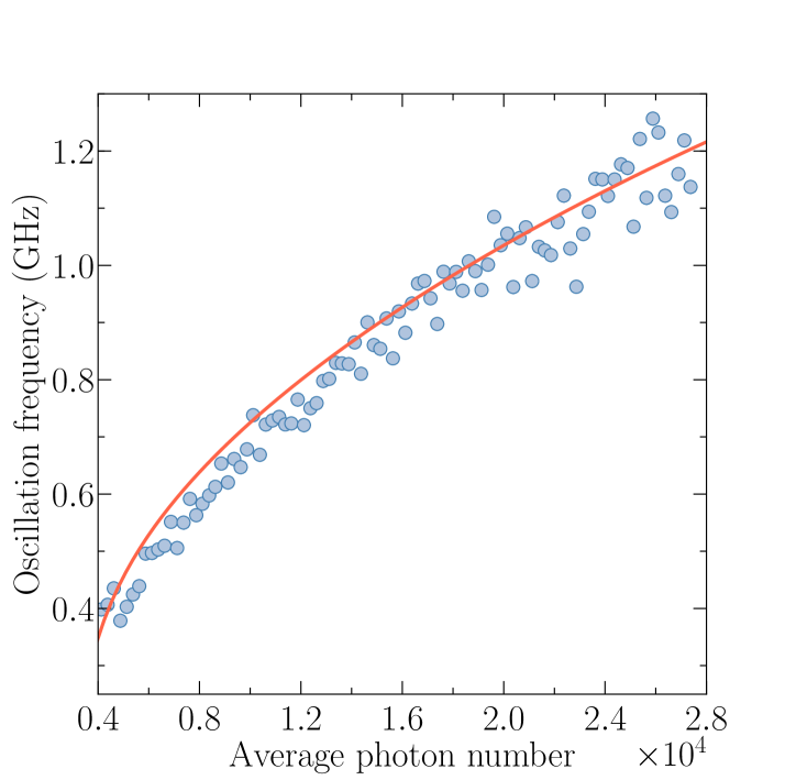
Figure 4: Oscillation frequency $\omega^{(2)}$ of the second order correlation function $g^{(2)}(\tau)$ as a function of the average photon number $\langle n\rangle_{\infty}$ in the condensate, as measured in the experiment (dots) and predicted by a nonlinear rate equation model (solid line). See the main text for details. The parameter values are $M=5.17\cdot 10^{9}$, $\kappa=2.33$ GHz, $B_{\text{em}}=2.50\cdot 10^{-5}$ GHz, $B_{\text{em}}/B_{\text{abs}}\approx 57$ (Kennard-Stepanov relation corresponding to the cutoff wavelength of $\lambda_{c}=571.3$ nm), $\Gamma_{\downarrow}=0$.

Remarkably, despite the clear nonequilibrium signatures in $g^{(2)}(\tau)$, a spectral distribution which, within experimental accuracies, is indistinguishable from the thermal equilibrium Bose-Einstein distribution is attained (see Fig. 2). The physical origin of this seemingly contradictory behavior is that there is a (stationary) net flow of photons from the dye reservoir to the resonator and out to the environment, in such a way that the average photon number is constant and the photon gas reaches a thermal spectral distribution due to the thermal contact with the dye. Interestingly, our calculations show that the nonvanishing zero-delay second order correlations $g^{(2)}(0)>1$, from the grand canonical nature of the photon condensate, are (in the investigated limits) not affected by the nonequilibrium character of the system. However, the residual photon loss and pump do affect the temporal decay of the correlation function $g^{(2)}(\tau)$. This photon flow causes additional structure in the intensity correlations, as observed in the present work. A related behavior is known in nanoelectronic systems, e.g. current carrying, metallic nanowires, where the electron energy distribution is equilibrated from fast electron-electron collisions in the wire Steinbach et al. (1996).

V Conclusions

To conclude, we observed an oscillatory behavior of grand canonical Bose-Einstein condensates by studying the second-order coherence of the emission of a dye microcavity. Its origin is traced back to the remnant driven-dissipative character of the light condensate. Our results show that even when the energy distribution of particles to good accuracy follows the predictions for thermal equilibrium, fluctuation dynamics depend sensitively on the openness of the system. We note that a related behavior can be observed in the hot-electron regime of electronic quantum wires at large bias voltage, where nonthermal noise, albeit not oscillatory, is induced by the current. Due to fast electron-electron collisions in the wire, it coexists with an equilibrium (Fermi-Dirac) distribution of the electron energy. Here we observe this phenomenon in a photon system for the first time.

The $g^{(2)}(\tau)$ oscillations observed in our photon condensates are reminiscent of relaxation oscillations in lasers. However, there are important differences. First, a laser is in a state far from equilibrium with nonthermal spectral distribution. In contrast, our system is operated in a near-equilibrium state with a thermal Bose-Einstein distribution, but clearly nonequilibrium dynamics of the photon number correlations. Secondly, in a steady-state laser $g^{(2)}(\tau)=1$ for all times. This means that oscillations of $g^{(2)}(\tau)$ do not occur unless the system is perturbed from outside, such as in the initial increase of the cavity photon number when a laser is turned on. For our system, when it is not operated with a very small relative size of the reservoir, the steady state is characterized by $g^{(2)}(0)>1$. These fluctuations of the grand canonical system are responsible for the excitation of the oscillations.

Our findings open up new avenues for further investigations of the open-system dynamics of grand canonical photon condensates. In the future, the experiments may be extended to further study the regime with stronger dissipation and drive. In addition, the second-order correlations can be used as a tool to sensitively characterize the system parameters. In a lattice with several coupled grand canonical photon condensates, a variety of new dynamical phases may be expected.

Note added in proof. Recently, a report on related experiments with a dye-microcavity subject to short pulsed picosecond laser pump irradiation appeared Walker2019 .

APPENDIX: TRUNCATION OF HIERARCHY

In this Appendix, we present details on the hierarchy of the equations of motion for the expectation values of successively increasing order. These will be calculated from the master equation Kirton and Keeling (2013)

$$\begin{split}\dot{\rho}&=\frac{\kappa}{2}\mathcal{L}[a]\rho+\frac{1}{2}\sum_{m=1}^{M}\Big{\{}\Gamma_{\uparrow}\mathcal{L}[\sigma^{+}_{m}]+\Gamma_{\downarrow}\mathcal{L}[\sigma^{-}_{m}]\\ &+B_{\text{em}}\mathcal{L}[a^{\dagger}\sigma^{-}_{m}]+B_{\text{abs}}\mathcal{L}[a\sigma^{+}_{m}]\Big{\}}\rho.\end{split}$$ (20)

Assuming that the molecules are all identical, one can replace the sum over the $M$ molecules in the equation for the photon occupation $\langle a^{\dagger}a\rangle$ by a factor of $M$ and find

$$\begin{split}\partial_{t}{\langle a^{\dagger}a\rangle}&=-\kappa\langle a^{\dagger}a\rangle-\frac{M}{2}B_{\text{abs}}\langle a^{\dagger}a\left(1-\sigma^{z}\right)\rangle\\ &+\frac{M}{2}B_{\text{em}}\langle aa^{\dagger}\left(1+\sigma^{z}\right)\rangle,\end{split}$$ (21a)

$$\begin{split}\partial_{t}{\langle\sigma^{z}\rangle}&=\Gamma_{\uparrow}\left(1-\langle\sigma^{z}\rangle\right)-\Gamma_{\downarrow}\left(1+\langle\sigma^{z}\rangle\right)\\ &+B_{\text{abs}}\langle a^{\dagger}a\left(1-\sigma^{z}\right)\rangle-B_{\text{em}}\langle aa^{\dagger}\left(1+\sigma^{z}\right)\rangle,\end{split}$$ (21b)

where we have dropped the molecule index $m$. Multiplying Eq. (21b) by $M/2$ and using $M\partial_{t}\langle\sigma^{z}\rangle/2=\partial_{t}\langle M_{\uparrow}\rangle$, $\langle\sigma^{+}\sigma^{-}\rangle=\langle 1+\sigma^{z}\rangle/2=\langle m\rangle/M$, $\langle\sigma^{-}\sigma^{+}\rangle=\langle 1-\sigma^{z}\rangle/2=\langle M-m\rangle/M$, and $\langle nM_{\uparrow}\rangle\approx\langle n\rangle\langle M_{\uparrow}\rangle$, we arrive at Eqs. (4). The latter approximation is excellent for large systems: while $\Delta g^{(2)}_{n,\,M_{\uparrow}}(0)=\langle M_{\uparrow}n\rangle_{\infty}-\langle n\rangle_{\infty}\langle M_{\uparrow}\rangle_{\infty}$ does not vanish in general, its influence on $\langle n\rangle_{\infty}$, $\langle M_{\uparrow}\rangle_{\infty}$ turns out to be negligible.

Accordingly, the equations of motion of the next-order expectation values in Eqs. (21) are given by

$$\begin{split}\partial_{t}\langle a^{\dagger}a^{\dagger}aa\rangle&=-2\kappa\langle a^{\dagger}a^{\dagger}aa\rangle-2MB_{\text{abs}}\langle a^{\dagger}a^{\dagger}aa\sigma^{-}\sigma^{+}\rangle+2MB_{\text{em}}\left(\langle a^{\dagger}a^{\dagger}aa\sigma^{+}\sigma^{-}\rangle+2\langle a^{\dagger}a\sigma^{+}\sigma^{-}\rangle\right),\end{split}$$ (22a)

$$\begin{split}\partial_{t}{\langle a^{\dagger}a\sigma^{+}\sigma^{-}\rangle}&=-\kappa\langle a^{\dagger}a\sigma^{+}\sigma^{-}\rangle+\Gamma_{\uparrow}\langle a^{\dagger}a\sigma^{-}\sigma^{+}\rangle-\Gamma_{\downarrow}\langle a^{\dagger}a\sigma^{+}\sigma^{-}\rangle\\ &+B_{\text{abs}}\langle a^{\dagger}a^{\dagger}aa\sigma^{-}\sigma^{+}\rangle-B_{\text{em}}\left(\langle a^{\dagger}a^{\dagger}aa\sigma^{+}\sigma^{-}\rangle+2\langle a^{\dagger}a\sigma^{+}\sigma^{-}\rangle\right)\\ &-(M-1)B_{\text{abs}}\langle a^{\dagger}a\sigma^{+}\sigma^{-}\tilde{\sigma}^{-}\tilde{\sigma}^{+}\rangle+(M-1)B_{\text{em}}\langle aa^{\dagger}\sigma^{+}\sigma^{-}\tilde{\sigma}^{+}\tilde{\sigma}^{-}\rangle,\end{split}$$ (22b)

$$\begin{split}\partial_{t}\langle\sigma^{+}\sigma^{-}\tilde{\sigma}^{+}\tilde{\sigma}^{-}\rangle&=\Gamma_{\uparrow}\left(\langle\sigma^{-}\sigma^{+}\tilde{\sigma}^{+}\tilde{\sigma}^{-}\rangle+\langle\sigma^{+}\sigma^{-}\tilde{\sigma}^{-}\tilde{\sigma}^{+}\rangle\right)-2\Gamma_{\downarrow}\langle\sigma^{+}\sigma^{-}\tilde{\sigma}^{+}\tilde{\sigma}^{-}\rangle\\ &+B_{\text{abs}}\left(\langle a^{\dagger}a\sigma^{-}\sigma^{+}\tilde{\sigma}^{+}\tilde{\sigma}^{-}\rangle+\langle a^{\dagger}a\sigma^{+}\sigma^{-}\tilde{\sigma}^{-}\tilde{\sigma}^{+}\rangle\right)-2B_{\text{em}}\langle aa^{\dagger}\sigma^{+}\sigma^{-}\tilde{\sigma}^{+}\tilde{\sigma}^{-}\rangle.\end{split}$$ (22c)

The Pauli matrices $\tilde{\sigma}^{\pm}$ describe any molecule that is not identical to $\sigma^{\pm}$. Under the assumption that the total density matrix of the molecules is an incoherent mixture of all states corresponding to an excitation number of $M_{\uparrow}$ Kirton and Keeling (2015), which will be the case for the steady-state density matrix of the master equation (20), one can show that the expectation values of four Pauli matrices decompose as

$$\begin{split}M(M-1)\langle\sigma^{+}\sigma^{-}\tilde{\sigma}^{+}\tilde{\sigma}^{-}\rangle&=\langle M_{\uparrow}^{2}\rangle-\langle M_{\uparrow}\rangle,\\ M(M-1)\langle\sigma^{+}\sigma^{-}\tilde{\sigma}^{-}\tilde{\sigma}^{+}\rangle&=M\langle M_{\uparrow}\rangle-\langle M_{\uparrow}^{2}\rangle.\end{split}$$ (23)

Then the truncation of Eqs. (22) can be performed rigorously by expanding the highest-order expectation values according to

$$\begin{split}&M(M-1)\langle aa^{\dagger}\sigma^{+}\sigma^{-}\tilde{\sigma}^{+}\tilde{\sigma}^{-}\rangle\\ &=\langle(n+1)(M_{\uparrow}^{2}-M_{\uparrow})\rangle\\ &=\langle nM_{\uparrow}^{2}\rangle-\langle nM_{\uparrow}\rangle+\langle M_{\uparrow}^{2}\rangle-\langle M_{\uparrow}\rangle,\end{split}$$

and using the relation

$$\langle nM_{\uparrow}^{2}\rangle=2\langle M_{\uparrow}\rangle\langle nM_{\uparrow}\rangle+\langle n\rangle\langle M_{\uparrow}^{2}\rangle-2\langle n\rangle\langle M_{\uparrow}\rangle^{2}.$$ (24)

In this manner, after multiplying Eq. (22b) by a factor of $M$ and Eq. (22c) by $M(M-1)$, one obtains Kirton and Keeling (2015)

$$\begin{split}\partial_{t}\langle n^{2}\rangle&=\partial_{t}\langle a^{\dagger}aa^{\dagger}a\rangle=\partial_{t}\langle a^{\dagger}a^{\dagger}aa\rangle+\partial_{t}\langle a^{\dagger}a\rangle\\ &=\kappa(\langle n\rangle-2\langle n^{2}\rangle)-B_{\text{abs}}\left[2\langle n^{2}\rangle(M-\langle M_{\uparrow}\rangle)+4\langle M_{\uparrow}\rangle\langle n\rangle^{2}-4\langle n\rangle\langle nM_{\uparrow}\rangle-\langle n(M-M_{\uparrow})\rangle\right]\\ &+B_{\text{em}}\left[4\langle n\rangle\langle nM_{\uparrow}\rangle+2\langle M_{\uparrow}\rangle\langle n^{2}\rangle-4\langle M_{\uparrow}\rangle\langle n\rangle^{2}+\langle(3n+1)M_{\uparrow}\rangle\right],\end{split}$$ (25a)

$$\begin{split}\partial_{t}\langle nM_{\uparrow}\rangle&=M\partial_{t}{\langle a^{\dagger}a\sigma^{+}\sigma^{-}\rangle}\\ &=-\kappa\langle nM_{\uparrow}\rangle+\Gamma_{\uparrow}\langle n(M-M_{\uparrow})\rangle-\Gamma_{\downarrow}\langle nM_{\uparrow}\rangle\\ &+B_{\text{abs}}\left[2\langle M_{\uparrow}\rangle\langle n\rangle(\langle n\rangle-\langle M_{\uparrow}\rangle)-M(\langle n\rangle+\langle nM_{\uparrow}\rangle)+\langle n\rangle\langle M_{\uparrow}^{2}\rangle+2(\langle M_{\uparrow}\rangle-\langle n\rangle+\tfrac{1}{2})\langle nM_{\uparrow}\rangle+(M-\langle M_{\uparrow}\rangle)\langle n^{2}\rangle\right]\\ &+B_{\text{em}}\left[2\langle M_{\uparrow}\rangle\langle n\rangle(\langle n\rangle-\langle M_{\uparrow}\rangle)-\langle M_{\uparrow}\rangle+(\langle n\rangle+1)\langle M_{\uparrow}^{2}\rangle+2(\langle M_{\uparrow}\rangle-\langle n\rangle-1)\langle nM_{\uparrow}\rangle-\langle M_{\uparrow}\rangle\langle n^{2}\rangle\right],\end{split}$$ (25b)

$$\begin{split}\partial_{t}\langle M_{\uparrow}^{2}\rangle&=M(M-1)\partial_{t}\langle\sigma^{+}\sigma^{-}\tilde{\sigma}^{+}\tilde{\sigma}^{-}\rangle+\partial_{t}\langle M_{\uparrow}\rangle\\ &=2\Gamma_{\uparrow}\left(M\langle M_{\uparrow}\rangle+M-\langle M_{\uparrow}\rangle-\langle M_{\uparrow}^{2}\rangle\right)+\Gamma_{\downarrow}\left(\langle M_{\uparrow}\rangle-2\langle M_{\uparrow}^{2}\rangle\right)\\ &+B_{\text{abs}}\left((2M-1)\langle nM_{\uparrow}\rangle+M\langle n\rangle-4\langle M_{\uparrow}\rangle\langle nM_{\uparrow}\rangle-2\langle n\rangle\langle M_{\uparrow}^{2}\rangle+4\langle n\rangle\langle M_{\uparrow}\rangle^{2}\right)\\ &-B_{\text{em}}\left(4\langle M_{\uparrow}\rangle\langle nM_{\uparrow}\rangle+2\langle n\rangle\langle M_{\uparrow}^{2}\rangle-4\langle n\rangle\langle M_{\uparrow}\rangle^{2}+2\langle M_{\uparrow}^{2}\rangle-(\langle n\rangle+1)\langle M_{\uparrow}\rangle\right).\end{split}$$ (25c)

As mentioned in the main text, the steady-state solution of these equations is required for the initial values of the dynamics of the second-order correlation functions.

References

- Pitaevskiĭ and Stringari (2003) L. P. Pitaevskiĭ and S. Stringari, Bose-Einstein Condensation, International Series of Monographs on Physics, Vol. 116 (Clarendon Press, Oxford, 2003).
- Bloch et al. (2008) I. Bloch, J. Dalibard, and W. Zwerger, Rev. Mod. Phys. 80, 885 (2008).
- Anderson et al. (1995) M. H. Anderson, J. R. Ensher, M. R. Matthews, C. E. Wieman, and E. A. Cornell, Science 269, 198 (1995).
- Davis et al. (1995) K. B. Davis, M.-O. Mewes, M. R. Andrews, N. J. van Druten, D. S. Durfee, D. M. Kurn, and W. Ketterle, Phys. Rev. Lett. 75, 3969 (1995).
- Kasprzak et al. (2006) J. Kasprzak, M. Richard, S. Kundermann, A. Baas, P. Jeambrun, J. M. J. Keeling, F. M. Marchetti, M. H. Szymańska, R. André, J. L. Staehli, V. Savona, P. B. Littlewood, B. Deveaud, and S. Le Dang, Nature 443, 409 (2006).
- Balili et al. (2007) R. Balili, V. Hartwell, D. Snoke, L. Pfeiffer, and K. West, Science 316, 1007 (2007).
- Klaers et al. (2010) J. Klaers, J. Schmitt, F. Vewinger, and M. Weitz, Nature 468, 545 (2010).
- Marelic and Nyman (2015) J. Marelic and R. A. Nyman, Phys. Rev. A 91, 033813 (2015).
- Greveling et al. (2018) S. Greveling, K. L. Perrier, and D. van Oosten, Phys. Rev. A 98, 013810 (2018).
- Fujiwara et al. (1970) I. Fujiwara, D. ter Haar, and H. Wergeland, J. Stat. Phys. 2, 329 (1970).
- Ziff et al. (1977) R. M. Ziff, G. E. Uhlenbeck, and M. Kac, Phys. Rep. 32, 169 (1977).
- Klaers et al. (2012) J. Klaers, J. Schmitt, T. Damm, F. Vewinger, and M. Weitz, Phys. Rev. Lett. 108, 160403 (2012).
- Sob’yanin (2012) D. N. Sob’yanin, Phys. Rev. E 85, 061120 (2012).
- Zamora et al. (2017) A. Zamora, L. M. Sieberer, K. Dunnett, S. Diehl, and M. H. Szymańska, Phys. Rev. X 7, 041006 (2017).
- Vorberg et al. (2018) D. Vorberg, R. Ketzmerick, and A. Eckardt, Phys. Rev. A 97, 063621 (2018).
- Deng et al. (2010) H. Deng, H. Haug, and Y. Yamamoto, Rev. Mod. Phys. 82, 1489 (2010).
- Byrnes et al. (2014) T. Byrnes, N. Y. Kim, and Y. Yamamoto, Nature Physics 10, 803 (2014).
- Sun et al. (2017) Y. Sun, P. Wen, Y. Yoon, G. Liu, M. Steger, L. N. Pfeiffer, K. West, D. W. Snoke, and K. A. Nelson, Phys. Rev. Lett. 118, 016602 (2017).
- Kirton and Keeling (2013) P. Kirton and J. Keeling, Phys. Rev. Lett. 111, 100404 (2013).
- Schmitt et al. (2015) J. Schmitt, T. Damm, D. Dung, F. Vewinger, J. Klaers, and M. Weitz, Phys. Rev. A 92, 011602(R) (2015).
- Schmitt et al. (2014) J. Schmitt, T. Damm, D. Dung, F. Vewinger, J. Klaers, and M. Weitz, Phys. Rev. Lett. 112, 030401 (2014).
- Lakowicz (2006) J. R. Lakowicz, Principles of Fluorescence Spectroscopy, 3rd ed. (Springer, Boston, MA, 2006).
- Angelis et al. (2000) E. D. Angelis, F. D. Martini, and P. Mataloni, J. Opt. B 2, 149 (2000).
- Yokoyama and Brorson (1989) H. Yokoyama and S. D. Brorson, J. Appl. Phys. 66, 4801 (1989).
- Takemura et al. (2012) N. Takemura, J. Omachi, and M. Kuwata-Gonokami, Phys. Rev. A 85, 053811 (2012).
- Brennecke et al. (2013) F. Brennecke, R. Mottl, K. Baumann, R. Landig, T. Donner, and T. Esslinger, Proc. Nat. Acad. Sci. USA 110, 11763 (2013).
- Berner et al. (2018) J. Berner, B. Müller, J. R. Gomez-Solano, M. Krüger, and C. Bechinger, Nat. Commun. 9, 999 (2018).
- Moradi et al. (2018) T. Moradi, M. B. Harouni, and M. H. Naderi, Sci. Rep. 8, 12435 (2018).
- Klaers et al. (2011) J. Klaers, J. Schmitt, T. Damm, F. Vewinger, and M. Weitz, Appl. Phys. B 105, 17 (2011).
- Barroso et al. (1998) J. Barroso, A. Costela, I. Garcia-Moreno, and R. Sastre, Chem. Phys. 238, 257 (1998).
- Kirton and Keeling (2015) P. Kirton and J. Keeling, Phys. Rev. A 91, 033826 (2015).
- Keeling and Kirton (2016) J. Keeling and P. Kirton, Phys. Rev. A 93, 013829 (2016).
- Marthaler et al. (2011) M. Marthaler, Y. Utsumi, D. S. Golubev, A. Shnirman, and G. Schön, Phys. Rev. Lett. 107, 093901 (2011).
- Radonjić et al. (2018) M. Radonjić, W. Kopylov, A. Balaž, and A. Pelster, New J. Phys. 20, 055014 (2018).
- Steinbach et al. (1996) A. H. Steinbach, J. M. Martinis, and M. H. Devoret, Phys. Rev. Lett. 76, 3806 (1996).
- (36) B. T. Walker, J. D. Rodrigues, H. S. Dhar, R. F. Oulton, F. Mintert, and R. A. Nyman, arXiv:1908.05568.