Population Predictive Checks

Abstract

Bayesian modeling helps applied researchers articulate assumptions about their data and develop models tailored for specific applications. Thanks to good methods for approximate posterior inference, researchers can now easily build, use, and revise complicated Bayesian models for large and rich data. These capabilities, however, bring into focus the problem of model criticism. Researchers need tools to diagnose the fitness of their models, to understand where they fall short, and to guide their revision. In this paper we develop a new method for Bayesian model criticism, the population predictive check (pop-pc). pop-pcs are built on posterior predictive checks (ppcs), a seminal method that checks a model by assessing the posterior predictive distribution on the observed data. However, ppcs use the data twice—both to calculate the posterior predictive and to evaluate it—which can lead to overconfident assessments of the quality of a model. pop-pcs, in contrast, compare the posterior predictive distribution to a draw from the population distribution, a heldout dataset. This method blends Bayesian modeling with frequenting assessment. Unlike the ppc, we prove that the pop-pc is properly calibrated. Empirically, we study pop-pcs on classical regression and a hierarchical model of text data.

1 Introduction

Thanks to good algorithms for approximate Bayesian inference and good software for general Bayesian modeling, statisticians can now explore and develop a large variety of Bayesian models for a given problem. This new ease with which we can model data has turned the practice of Bayesian modeling into an iterative cycle (Blei,, 2014; Gelman et al.,, 1995, 2020). More complex models are constructed from simpler ones, and we can evaluate earlier model “drafts” to guide the structure of subsequent revisions. But this iterative process for model-building brings into sharp focus the problem of model criticism. How do we navigate the space of models we can use for a problem? How do we decide when a model needs to change? In this paper, we develop the population predictive check (pop-pc), a new method of model criticism.

One of the key tools for Bayesian model criticism is the posterior predictive check (ppc) (Guttman,, 1967; Rubin,, 1984). In a ppc, we locate the observed data within the posterior predictive distribution, a reference distribution that is determined by the model under consideration. The spirit of a ppc is to formalize the following heuristic: “If my model is good, then its posterior predictive distribution will generate data that looks like my observations (filtered through a diagnostic function).”

Consider an observed dataset $\bm{y}^{\mathrm{obs}}$ and a model with latent variables $\bm{\theta}$,

$$\mathrm{p}(\bm{\theta},\bm{y}^{\mathrm{obs}})=\mathrm{p}(\bm{\theta})\mathrm{p}(\bm{y}^{\mathrm{obs}}\,|\,\bm{\theta}).$$ (1)

The prior is $\mathrm{p}(\bm{\theta})$; the likelihood is $\mathrm{p}(\bm{y}^{\mathrm{obs}}\,|\,\bm{\theta})$. The model and data combine to form the posterior $\mathrm{p}(\bm{\theta}\,|\,\bm{y}^{\mathrm{obs}})$, which helps form the posterior predictive distribution,

$$\mathrm{p}(\bm{y}^{\mathrm{rep}}\,|\,\bm{y}^{\mathrm{obs}})=\int\mathrm{p}(\bm{y}^{\mathrm{rep}}\,|\,\bm{\theta})\mathrm{p}(\bm{\theta}\,|\,\bm{y}^{\mathrm{obs}})\mathop{}\!\mathrm{d}\bm{\theta}.$$ (2)

Here the variable $\bm{y}^{\mathrm{rep}}$ denotes replicated data.

To implement a ppc, we first choose a diagnostic statistic $d(\bm{y})$, a way to measure discrepancy between a dataset $\bm{y}$ and the model. An example diagnostic is the average squared distance to the posterior mean, $d(\bm{y})=\frac{1}{n}\sum_{i=1}^{n}(y_{i}-\mathrm{E}\left[Y\,|\,\bm{y}\right])^{2}$. The ppc then locates $d(\bm{y}^{\mathrm{obs}})$ in the reference distribution of $d(\bm{y}^{\mathrm{rep}})$, the posterior predictive from Equation 2. One common approach is with a posterior predictive $p$-value,

$$p_{\mathrm{ppc}}=\mathrm{p}(d(\bm{y}^{\mathrm{rep}})\geq d(\bm{y}^{\mathrm{obs}})\,|\,\bm{y}^{\mathrm{obs}}).$$ (3)

Bayarri and Morales, (2003) discusses other ways to measure surprise, and Gelman et al., (1996); Gelman, (2004) discuss visual approaches to checking the model.

But there is a crucial issue with the ppc—it uses the data twice. The data are first used to construct the reference distribution of the diagnostic, the posterior predictive distribution of Equation 2. The data are then used again in the observed diagnostic $d(\bm{y}^{\mathrm{obs}})$, which is located within the reference, such as with the $p$-value of Equation 3. Essentially, a ppc checks how “close” $d(\bm{y}^{\mathrm{obs}})$ is to $d(\bm{y}^{\mathrm{rep}})$, a quantity that also depends on $\bm{y}^{\mathrm{obs}}$. The issue is that they can be close regardless of whether the model is correct.

This paper introduces a solution to this “double use of the data” problem. The population predictive check (pop-pc) is a new method for Bayesian model criticism, one that combines the Bayesian ppc with the frequentist idea of the population distribution. The premise of the pop-pc is this: “If my model is good, then data drawn from the posterior predictive distribution will look like a draw from the true population.”

Along with the data, model, and posterior predictive, consider new data drawn from the true population distribution $\bm{y}^{\mathrm{new}}\sim F$. The pop-pc locates $d(\bm{y}^{\mathrm{new}})$ in the posterior predictive distribution of $d(\bm{y}^{\mathrm{rep}})$. As a $p$-value, a pop-pc is

$$p_{\mathrm{pop}}=\mathrm{p}(d(\bm{y}^{\mathrm{rep}})\geq d(\bm{y}^{\mathrm{new}})\,|\,\bm{y}^{\mathrm{obs}},\bm{y}^{\mathrm{new}}),$$ (4)

where $\bm{y}^{\mathrm{rep}}\sim\mathrm{p}(\bm{y}^{\mathrm{rep}}\,|\,\bm{y}^{\mathrm{obs}})$. This quantity no longer uses the data twice.

To implement a pop-pc, we split the data into $\bm{y}=(\bm{y}^{\mathrm{obs}},\bm{y}^{\mathrm{new}})$, assuming $\bm{y}^{\mathrm{new}}$ is an independent draw from the population distribution. We then calculate Equation 4. As with the ppc, the modeler can use other measures of surprise or visual checks. Figure 1 dispalys a schematic which relates the pop-pc to both the prior predictive check (Box,, 1980) and the ppc (Guttman,, 1967; Rubin,, 1984).

Why should a modeler avoid the double use of the data? Why prefer the pop-pc of Equation 4 to the ppc of Equation 3? We can understand the consequences of this practice by examining some of the frequentist properties of a predictive check. Suppose we repeatedly sample an observed dataset, and then check a model; note this is a frequentist situation. We define a model to be “correct” when its posterior predictive distribution is equal to (or approaches) the distribution of the observations; this is the conceit for both a ppc and a pop-pc.

Now consider the sampling distribution of the ppc $p$-value. There are two consequences of its double use of the data. First, the ppc $p$-value may be likely to retain an incorrect model; it may suffer from low power. Second, the ppc $p$-value may be overconfident about the correct model; it is not calibrated. In contrast, the pop-pc does not suffer from these issues. Theoretically, under certain assumptions, we prove that the pop-pc is calibrated. In a specific setup, we prove that the pop-pc rejects an incorrect model with probability one in the infinite data limit; in contrast, we show that calibrated versions of the ppc (Robins et al.,, 2000; Hjort et al.,, 2006) fail to reject the model. Empirically, we find the pop-pc is better calibrated than the ppc. We also find that it has higher power–a pop-pc can more easily detect an incorrect model than either a ppc or calibrated ppcs (Robins et al.,, 2000; Hjort et al.,, 2006).

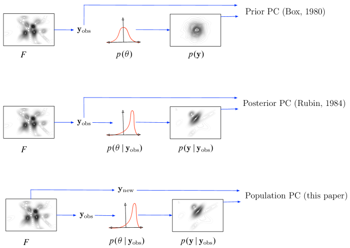
Figure 1: A schematic diagram that relates Box, (1980), Rubin, (1984), and this paper. This diagram posits the data come from an unknown population distribution. Box, (1980) uses the data as reference in the marginal distribution induced by the model (top); Rubin, (1984) uses the data as reference in the posterior predictive distribution induced by the model (middle); our method uses a draw from the population as a reference in the posterior predictive distribution (bottom).

The paper is organized as follows. Section 1.1 discusses the historical development of Bayesian model evaluation and how pop-pcs fit in. Section 2 develops the pop-pc and provides an illustrative example. Section 3 proves that the pop-pc $p$-value is calibrated. Section 4 illustrates how the “double use of the data” affects the power of ppcs, unlike the pop-pc. Further, calibrating ppcs does not resolve this power issue. Section 5 demonstrates the pop-pc empirically on a regression model and a hierarchical document model. Section 6 concludes the paper.

1.1 Related work

This work builds on predictive checks, which are part of the larger literature on Bayesian model criticism. Predictive checks locate the observations in a model-based distribution of data, the reference distribution. A brief history: Inspired by the earlier ideas of Geisser, (1975), Box, (1980) used the prior predictive distribution as the reference. This is a prior predictive check, which is useful for checking the conflict between prior and likelihood (Evans and Moshonov,, 2006). Later, Rubin, (1984) mimicked Box’s framework, but replaced the prior predictive with the posterior predictive; this strategy is both more practical for diagnosing models and one that is, in Rubin’s language, “Bayesianly justifiable.” Guttman, (1967) proposed the same approach. Finally, Gelman et al., (1996) showed how to develop diagnostic functions of the data—termed realized discrepancy functions—that depend on both a data set and the latent variables.

To resolve the “double use” problem, researchers have proposed a range of strategies. One strand of research proposes to calibrate a posterior predictive check (ppc) $p$-value post-hoc by using its empirical distribution (Robins et al.,, 2000; Hjort et al.,, 2006). However, calibration by itself does not necessarily improve the power of the check, as we will show in Sections 4 and 5.

Alternatively, Bayarri and Berger, (2000) proposes the partial predictive check. The partial predictive check calculates a predictive reference distribution that does not depend on the diagnostic, thereby removing the correlation between the diagnostic and the reference. Consequently, the partial predictive check is calibrated (Bayarri and Berger,, 2000; Robins et al.,, 2000). Finally, Johnson, (2007) proposed to use pivotal diagnostics to ensure the diagnostic and reference distribution are uncorrelated.

The population predictive check (pop-pc) can be viewed as a prior predictive check where the prior is updated based on a subset of the data. Note that this idea of using data-dependent priors was also applied to the idea of intrinsic Bayes factors (Berger and Pericchi,, 1996). The intrinsic Bayes factor first calculates a posterior using only a subset of the data. This posterior is then treated as a prior, and the Bayes factor is calculated using the remaining data. In a similar way, the pop-pc first calculates the posterior given the observed data, and then treats this posterior as a prior in a prior predictive check of the new data.

The pop-pc also has close connections to the partial predictive check (Bayarri and Berger,, 2000). Specifically, when the partial PC diagnostic uses only a subset of the data, the partial PC can coincide with the pop-pc (see Appendix D of the Supplementary Material for an example). In certain cases, a partial posterior check which computes the diagnostic with only a subset of the data may be more efficient than a pop-pc. This efficiency is because a partial predictive check may only remove a sufficient statistic of this subset of the data, instead of the entire subset as in the pop-pc. A drawback of the partial predictive check, however, is that it can be difficult to calculate, and requires re-calculation for each diagnostic function. Meanwhile, a pop-pc is simple to implement, and the inferred posterior can be used to check many different diagnostic functions. A further limitation of the partial predictive check is that it can revert to the prior predictive check when the diagnostic contains the sufficient statistics of the model (see Appendix D of the Supplementary Material for an example).

Another closely related work is Gelfand et al., (1992), which develops cross-validated checks. A cross-validated check iteratively holds out each data point, conditioning on the remaining data, and compares samples from the corresponding posterior predictive distribution to the held-out point. Similar strategies are discussed in Draper, (1996); Marshall and Spiegelhalter, (2003); Larsen and Lu, (2007). In its relation to these other data-split checks, this paper provides a theoretical understanding and empirical evaluation for this class of methods.

Finally, in an independent and concurrent paper, Li and Huggins, (2022) identifies that a previous definition of the pop-pc (pop-pc-v1, see Appendix B of the Supplementary Material for details) is not calibrated, and proposes the split predictive check (spc). In revising this paper, we identified the same issue with pop-pc-v1, which we have resolved by updating it to its form in Equation 5. This pop-pc is the same as the single spc of Li and Huggins, (2022), and the proof here that it is calibrated (Theorem 1) is also similar to the proof of calibration in Li and Huggins, (2022) for the spc (their Theorem 3.1(1) for the case where the model is true). (The proofs are similar because both build on the work of Robins et al., (2000).)

Li and Huggins, (2022) and this paper present similar methods, but complementary perspectives. Li and Huggins, (2022) shows the SPC has asymptotic power of 1 under moderate-to-major model misspecification. It also proposes the divided spc, which considers spc $p$-values for multiple different splits of the data. In this paper, we examine the “double use of the data” problem of the ppc in greater detail. Specifically, we illustrate that post-hoc empirical calibration procedures for the ppc, while uniform under the null, do not resolve the “double use of the data” problem in terms of detecting model misspecification. Finally, we consider different diagnostics from Li and Huggins, (2022) - the $\chi^{2}$ diagnostic and latent Dirichlet allocation log-likelihood - and we provide empirical evidence that they are calibrated; these diagnostics are not covered by the calibration theory for the pop-pc, nor the spc.

2 Population Predictive Checks

The pop-pc checks a Bayesian model by considering a true population distribution: “If my model is good then data drawn from the posterior predictive distribution will look like a draw from the true population (filtered through a diagnostic function).”

The ingredients of a pop-pc are observed data $\bm{y}^{\mathrm{obs}}$, replicated data $\bm{y}^{\mathrm{rep}}$ from the posterior predictive distribution (Equation 2), and new data $\bm{y}^{\mathrm{new}}$, drawn from the true population distribution $F$. As for a ppc, each check involves a diagnostic statistic $d(\bm{y})$, which measures misfit between $\bm{y}$ and the model. The pop-pc uses new data $\bm{y}^{\mathrm{new}}$ to check if a draw from the population $F$ is close to the posterior predictive distribution $\mathrm{p}(\bm{y}^{\mathrm{rep}}\,|\,\bm{y}^{\mathrm{obs}})$, in terms of the diagnostic. If so, then the posterior predictive captures the data well, and the model passes the check.

Definition 1 (Population predictive check, pop-pc)

Consider observed data $\bm{y}^{\mathrm{obs}}$, its posterior predictive distribution $\mathrm{p}(\bm{y}^{\mathrm{rep}}\,|\,\bm{y}^{\mathrm{obs}})$, and a diagnostic statistic $d(\bm{y})$. Suppose we have $\bm{y}^{\mathrm{new}}$ drawn from the population distribution of the data. As a $p$-value, the population predictive check is:

$$p_{\mathrm{pop}}=\mathrm{p}(d(\bm{y}^{\mathrm{rep}})\geq d(\bm{y}^{\mathrm{new}})\,|\,\bm{y}^{\mathrm{obs}},\bm{y}^{\mathrm{new}}),$$ (5)

where $\bm{y}^{\mathrm{rep}}\sim\mathrm{p}(\bm{y}^{\mathrm{rep}}\,|\,\bm{y}^{\mathrm{obs}})$.

To implement a pop-pc, we split the data into $\bm{y}=(\bm{y}^{\mathrm{obs}},\bm{y}^{\mathrm{new}})$ and calculate Equation 5.

The diagnostic is a function of the data that measures model misfit. For example, one diagnostic is the conditional negative log-likelihood,

$$d(\bm{y})\triangleq-\frac{1}{n}\sum_{i=1}^{n}\log\mathrm{p}(y_{i}\,|\,\bm{y}^{\mathrm{obs}}).$$ (6)

In the context of a ppc, this diagnostic is discussed in Lewis and Raftery, (1996).

input:  data $\bm{y}=\{\bm{y}^{\mathrm{obs}},\bm{y}^{\mathrm{rep}}\}$, diagnostic $d(\cdot)$, # replicates $R$

output:  population predictive check $p$-value

for $r=1,\dots,R$ do

       draw samples from the posterior $\theta_{r}\sim\mathrm{p}(\theta|\bm{y}^{\mathrm{obs}})$;

       draw posterior predictive data $\bm{y}_{r}^{\mathrm{rep}}\sim\mathrm{p}(\bm{y}^{\mathrm{rep}}|\theta)$;

      

compute the empirical pop-pc $p$-value

$$p_{\mathrm{pop}} =\frac{1}{R}\sum_{r=1}^{R}1\left[d(\bm{y}_{r}^{\mathrm{rep}},\theta_{r})>d(\bm{y}^{\mathrm{new}},\theta_{r})\right];$$

return $p_{\mathrm{pop}}$

Algorithm 1 Population predictive check

Meng, (1994); Gelman et al., (1996) discuss realized diagnostics $d(\bm{y},\theta)$, those that also depend on the latent variables. A realized diagnostic measures the strength of the connection between latent variables and a data set. An example is the negative log-likelihood

$$d(\bm{y},\theta)\triangleq-\log\mathrm{p}(\bm{y}\,|\,\theta).$$ (7)

Consider a joint distribution of latent variables and data,

$$\mathrm{p}(\theta,\bm{y})=\mathrm{p}(\theta)\mathrm{p}(\bm{y}\,|\,\theta)$$ (8)

and a realized diagnostic $d(\theta,\bm{y})$. The pop-pc is

$$p_{\mathrm{pop}}=\mathrm{p}(d(\theta,\bm{y}^{\mathrm{rep}})>d(\theta,\bm{y}^{\mathrm{new}})\,|\,\bm{y}^{\mathrm{obs}},\bm{y}^{\mathrm{new}}).$$ (9)

This probability is under a distribution that draws the latent variable from the posterior and the replicated data from the likelihood given the latent variable,

$$\mathrm{p}(\theta,\bm{y}^{\mathrm{rep}}\,|\,\bm{y}^{\mathrm{obs}})=\mathrm{p}(\theta\,|\,\bm{y}^{\mathrm{obs}})\mathrm{p}(\bm{y}^{\mathrm{rep}}\,|\,\theta).$$ (10)

The pop-pc procedure is detailed in Algorithm 1.

2.1 Example

To illustrate the pop-pc, we now apply a ridge regression model to synthetic data. The model is:

$$\bm{\theta} \sim\textrm{Normal}(0,c\bm{I}_{p}),$$ (11)

$$\sigma^{2} \sim\textrm{Inverse-Gamma}(1/2,1/2),$$ (12)

$$y_{i} \sim\textrm{Normal}(\bm{\theta}^{\top}\bm{x}_{i},\sigma^{2}),\quad i=1,\dots,n.$$ (13)

We take $n=50$ and $p=100$. The covariates, $\bm{x}_{i}$, are drawn as uniform random variables on $[0,1]$. Meanwhile, the true coefficients, $\theta$, have five entries equal to 3.5 and the remaining 95 entries drawn from a standard normal distribution. Consequently, the coefficients $\theta$ has many entries close to zero, and a few large entries.

How do we choose the prior variance parameter $c$? If $c$ is too large, the estimated coefficients will overfit to the data and not generalize well on new data. Here, we show that a pop-pc can detect this overfitting while a ppc cannot.

To check the model, we use the $\chi^{2}$ diagnostic function:

$$d(\bm{y},\bm{\theta},\sigma^{2})=\frac{1}{N}\sum_{i=1}^{N}\frac{(y_{i}-\mathrm{E}[y_{i}|\bm{\theta},\sigma^{2}])^{2}}{\text{Var}(y_{i}|\bm{\theta},\sigma^{2})},$$ (14)

which is a sum of standardized residuals. We conduct posterior inference using a Gibbs sampler.

Figure 2 shows the pop-pc and ppc $p$-values for different values of $c$. Also plotted is the mean squared error:

$$\text{MSE}=\mathbb{E}\left[\left(\theta_{0}-\theta\right)^{2}\right]$$ (15)

where the expectation is with respect to the posterior $\mathrm{p}(\theta|\bm{y},\bm{X})$ and $\theta_{0}$ is the true value of the coefficents.

When $c$ is small, there is more regularization of the coefficient estimates. This regularization prevents overfitting and results in small mean squared error. For these small values of $c$, both the ppc and pop-pc both correctly retain the model. When $c$ is large, however, there is less regularization of the coefficients. Consequently, the model overfits to the data and the MSE is large. For these large values of $c$, the pop-pc correctly rejects the model. The ppc, however, does not reject the model; the ppc does not detect overfitting, unlike the pop-pc.

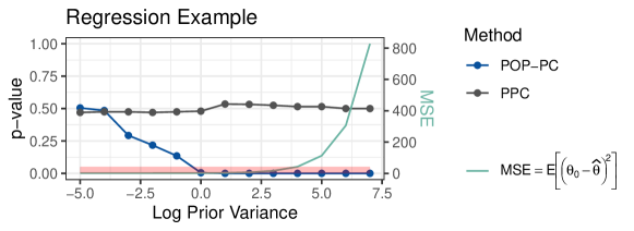
Figure 2: When the log prior variance $c$ is small, both the pop-pc and ppc correctly retain the model; when $c$ is large, the pop-pc correctly rejects the model, while the ppc incorrectly retains the model.

3 The asymptotic distribution of POP-PC $p$-values

In this section, we study the pop-pc $p$-value asymptotic sampling distribution. If a $p$-value is uniformly distributed when the model is correct, the $p$-value is said to be calibrated. For a class of diagnostic functions, we prove that the pop-pc $p$-value is calibrated (Theorem 1).

Calibration is a frequentist property, not a Bayesian one. Although the pop-pc checks Bayesian models, it is still important to determine if its $p$-values are calibrated. Calibration helps us interpret a $p$-value: If the distribution of $p$-values is uniform, a $p$-value of 0.4 would not be surprising, while if the distribution was concentrated around 0.5, the value 0.4 would be surprising. For a calibrated check, if we decide to reject a model when its $p$-value is less than $\alpha$, then the correct model will only fail such a check with that probability.

Before stating our pop-pc calibration result, we introduce some notation. The data are $\bm{y}=(y_{1},\dots,y_{n})$ where $y_{i}$ are mutually independent random variables with density $f(y;\theta)$ where $\theta\in\Theta\subset\mathbb{R}^{p}$.

We prove the pop-pc is calibrated for the same class of diagnostic functions $d(\bm{y})$ that are considered by Robins et al., (2000). Specifically, we consider diagnostic functions $d(\bm{y})$ that are asymptotically normal with asymptotic mean $\nu(\theta)$ and asymptotic variance $\sigma^{2}(\theta)$ when the model is correct (i.e. the density of $\bm{y}$ is $f(\bm{y};\theta)$):

$$n^{1/2}\left[\frac{d(\bm{y})-\nu(\theta)}{\sigma(\theta)}\right]\leadsto N(0,1),$$ (16)

where $\leadsto$ denotes convergence in distribution.

Theorem 1 proves that the pop-pc $p$-values are asymptotically uniform when the model is correct. Unlike the ppc, the pop-pc $p$-values are calibrated. Note our result relies on standard regularity conditions that are detailed in Section A.1 of the Supplementary Material.

Theorem 1

Assume Equation 16 holds and assume the regularity conditions detailed in Section A.1 of the Supplementary Material. Under the distribution $f(\bm{y};\theta_{0})$, the pop-pc $p$-value can be written as:

$$p_{\mathrm{pop}}(\bm{y}) =1-\Phi(Q)+o_{P}(1),$$ (17)

where $o_{P}(1)$ denotes a random variable converging to zero in probability, $\Phi$ is the standard normal cdf, and $Q\sim N(0,1)$. Consequently, the pop-pc $p$-values are calibrated.

The proof of Theorem 1 is in Section A.1 of the Supplementary Material.

Theorem 1 proves that pop-pc $p$-values are calibrated for realized diagnostics that are asymptotically normal. In experiments (Section 5) we consider diagnostics that are not asymptotically normal, including the $\chi^{2}$ diagnostic and the log-likelihood of latent Dirichlet allocation (Blei et al.,, 2003). With these diagnostics, we show empirically the pop-pc still has good calibration properties.

4 A comparison of predictive checks

In the previous section, we studied the pop-pc $p$-value distribution when the model is correct. In this section, we consider a specific setup to illustrate the properties of the pop-pc $p$-value when the model is incorrect. Under this setup, we show the pop-pc has high power–it detects this model misfit with probability one in the infinite data limit, while the ppc and calibrated versions of the ppc (Robins et al.,, 2000; Hjort et al.,, 2006) cannot detect this model misfit; that is, calibration by itself cannot improve the power of a test.

Suppose we have data $\bm{y}^{\mathrm{obs}}=\{y_{i}\}_{i=1}^{n}$. We posit a Gaussian model for the data:

$$y_{i}\sim N(\mu,\sigma^{2}),\quad i=1,\dots,n$$ (18)

with unknown mean $\mu\in\mathbb{R}$ and known $\sigma^{2}$.

We want to check the suitability of this Gaussian model with a Bayesian predictive check. Unlike a frequentist hypothesis test, the parameters of the model are not set to pre-specified values. That is, in Equation 18 we are not checking a specific value of the mean $\mu$, but the appropriateness of the Gaussian model.

A ppc checks whether the posited data distribution, combined with a prior, results in posterior predictive distributions that are consistent with the data.

In this section, we consider a specific alternative data distribution that would not fall in the Gaussian model eq. 18, so we can explicitly compare the power of predictive checks. This data distribution is a Cauchy distribution with location $x_{0}\in\mathbb{R}$ and scale $\gamma=1$:

$$y_{i}\sim\text{Cauchy}(x_{0},1),\quad i=1,\dots,n.$$ (19)

4.1 Posterior predictive checks

We first consider the distribution of a ppc $p$-value which checks the model Equation 18. For a diagnostic, we take the mean $d(\bm{y}^{\mathrm{obs}})=\overline{\bm{y}}^{\textrm{obs}}$. For a prior on $\mu$, we take $\mu\sim N(\mu_{0},\sigma_{0}^{2})$ with fixed hyperparameters $\mu_{0}\in\mathbb{R},\sigma_{0}^{2}\in\mathbb{R}^{+}$.

We show that this ppc $p$-value is degenerate at 0.5 regardless of whether the data is Gaussian or Cauchy. This degeneracy of the ppc $p$-value is problematic for both calibration and power. First, the $p$-value is not uniform and thus not calibrated. Secondly, the ppc $p$-value cannot detect model misfit when the data is actually Cauchy.

Concretely, the posterior predictive $p$-value with diagnostic $d(\bm{y}^{\mathrm{obs}})=\overline{\bm{y}}^{\textrm{obs}}$ is:

$$p_{\mathrm{ppc}}=\mathrm{p}(d(\bm{y}^{\mathrm{rep}})>d(\bm{y}^{\mathrm{obs}})|\bm{y}^{\mathrm{obs}}) =1-\Phi\left(\frac{\overline{\bm{y}}^{\mathrm{obs}}-\rho_{n}\overline{\bm{y}}^{\mathrm{obs}}-(1-\rho_{n})\mu_{0}}{\sqrt{(1+\rho_{n})\sigma^{2}/n}}\right),$$ (20)

where $\rho_{n}=\sigma_{0}^{2}/(\sigma_{0}^{2}+\sigma^{2}/n)$ (for details, see Appendix C of the Supplementary Material).

Ideally, the ppc would check some aspect of model misfit. However, the ppc in Equation 20 is only checking how “close” the posterior mean $\mathbb{E}[\mu|\bm{y}^{\mathrm{obs}}]=\rho_{n}\overline{\bm{y}}^{\mathrm{obs}}+(1-\rho_{n})\mu_{0}$ is to the MLE $\overline{\bm{y}}^{\mathrm{obs}}$. Whether the posterior mean is close to the MLE is a property of the model, unrelated to the fit of the model to the data. That is, the posterior mean can be close to the MLE, whether or not the underlying data is actually Gaussian.

To further illustrate this problem with the ppc, consider the asymptotic distribution of $p_{\mathrm{ppc}}$. In Equation 20, the numerator is $\overline{\bm{y}}^{\mathrm{obs}}-\rho_{n}\overline{\bm{y}}^{\mathrm{obs}}-(1-\rho_{n})\mu_{0}=O(1/n)$ and the denominator is $O(1/\sqrt{n})$. Consequently, the integrand goes to zero as $O(1/\sqrt{n})$ and the $p_{\mathrm{ppc}}$ converges to 0.5. What is important to note is that $p_{\mathrm{ppc}}$ converges to 0.5 regardless of whether the data is Gaussian or Cauchy.

We illustrated isses with the ppc for checking a Gaussian model with a mean diagnostic. In general, when does this degeneracy occur for ppc $p$-values? The ppc becomes degenerate when the diagnostic is perfectly correlated with the model parameters (Robins et al.,, 2000). More specifically, let $\theta(\bm{y}^{\mathrm{obs}})$ be the posterior mean of the model parameters, conditioned on the observed data. Under the conditions of Theorem 1, if the diagnostic $d(\bm{y}^{\mathrm{obs}})$ is perfectly correlated with $\theta(\bm{y}^{\mathrm{obs}})$, then the ppc will converge to 0.5. On the other hand, if the diagnostic is independent of $\theta(\bm{y}^{\mathrm{obs}})$, the ppc $p$-values are uniformly distributed and thus calibrated (Robins et al.,, 2000).

4.2 Empirical calibration of PPCs is insufficient

To fix the calibration of ppc $p$-values, a number of post-processing strategies have been proposed (Robins et al.,, 2000; Hjort et al.,, 2006). In this section, we show that such post-hoc calibration techniques do not improve the power of the ppc to detect model misfit.

Essentially, these calibration techniques cannot detect model misfit because for any random variable, we can calibrate it by using its cdf to transform it to a uniform distribution. If the original random variable does not detect model misfit, this transformation will not provide additional power to detect model misfit.

We make the above point more concrete by again considering Equation 18 and analyzing the following two post-hoc calibration methods:

• Robins et al., (2000) proposed to locate the observed ppc $p$-value in the empirical distribution of the ppc $p$-values. The empirical distribution of the ppc $p$-values is calculated by treating draws from the posterior predictive as replicates from the true model and then calculating their ppc $p$-values.

• Hjort et al., (2006) also propose to locate the observed ppc $p$-value in an empirical reference distribution. Unlike Robins et al., (2000), however, Hjort et al., (2006) use draws from the prior predictive distribution to calculate an empirical reference distribution (instead of draws from the posterior predictive).

First, we show that the Robins et al., (2000) empirically calibrated ppc $p$-value has the same distribution regardless of whether the data is Gaussian or Cauchy. Consequently, the check cannot detect model misfit.

The Robins et al., (2000) empirically calibrated ppc $p$-value is

$$\mathrm{p}\left(\text{ppc}(\bm{y}^{\mathrm{rep}})>\text{ppc}(\bm{y}^{\mathrm{obs}})|\bm{y}^{\mathrm{obs}}\right),$$ (21)

where

$$\text{ppc}(\bm{y}^{\mathrm{rep}})=\frac{1}{R}\sum_{r=1}^{R}\mathbbm{1}(\overline{\bm{y}}^{\mathrm{rep,rep}}_{r}>\overline{\bm{y}}^{\mathrm{rep}}),\quad{\bm{y}}^{\mathrm{rep,rep}}_{r}\sim\mathrm{p}(\bm{y}^{\mathrm{rep,rep}}|\bm{y}^{\mathrm{rep}}),$$ (22)

with $R$ draws from the posterior predictive distribution. Now, suppose $\rho_{n}\to 1$. Then, $\sqrt{n}(\overline{\bm{y}}^{\mathrm{rep,rep}}-\overline{\bm{y}}^{\mathrm{rep}})|\overline{\bm{y}}^{\mathrm{rep}}\sim N(0,2\sigma^{2})$. In this case, the probability that $\overline{\bm{y}}_{\textrm{rep,rep}}$ is greater than its mean is 0.5 and so the sum of indicators is a binomial random variable:

$$\sum_{r=1}^{R}\mathbbm{1}(\overline{\bm{y}}_{r}^{\mathrm{rep,rep}}>\overline{\bm{y}}^{\mathrm{rep}})\sim\text{Binomial}(R,0.5).$$ (23)

With the normal approximation to the binomial distribution,

$$\mathrm{p}\left(\text{ppc}(\bm{y}^{\mathrm{rep}})>\text{ppc}(\bm{y}^{\mathrm{obs}})|\bm{y}^{\mathrm{obs}}\right)=1-\Phi\left(2\sqrt{R}\left[\text{ppc}(\bm{y}^{\mathrm{obs}})-0.5\right]\right).$$ (24)

To determine the distribution of the empirically calibrated ppc, consider the distribution of $\text{ppc}(\bm{y}^{\mathrm{obs}})$. Similarly to Equation 23, for large $R$,

$$2\sqrt{R}[\text{ppc}(\bm{y}^{\mathrm{obs}})-0.5]\sim N(0,1),$$ (25)

again using the normal approximation to the binomial distribution. Then, the empirically calibrated ppc is uniform:

$$\mathrm{p}\left(\text{ppc}(\bm{y}^{\mathrm{rep}})>\text{ppc}(\bm{y}^{\mathrm{obs}})|\bm{y}^{\mathrm{obs}}\right)\sim U[0,1].$$ (26)

The key point is that the calibrated ppc is uniform regardless of whether the data is Gaussian or Cauchy. This is because for both data distributions, we have $\sqrt{n}(\overline{\bm{y}}^{\mathrm{rep,rep}}-\overline{\bm{y}}^{\mathrm{rep}})|\overline{\bm{y}}^{\mathrm{rep}}\sim N(0,2\sigma^{2})$ and $\sqrt{n}(\overline{\bm{y}}^{\mathrm{rep}}-\overline{\bm{y}}^{\mathrm{obs}})|\overline{\bm{y}}^{\mathrm{obs}}\sim N(0,2\sigma^{2})$. In other words, here, the empirically calibrated ppc does not depend on the underlying distribution of $\overline{\bm{y}}^{\mathrm{obs}}$ and so it cannot detect model misfit.

We now show that Hjort et al., (2006)’s calibrated $p$-value (cppp) also has the same distribution regardless of whether the data is Gaussian or Cauchy. Consequently, the check cannot detect model misfit.

The cppp is:

$$\mathrm{p}(\textrm{ppc}(\bm{y})>\textrm{ppc}(\bm{y}^{\mathrm{obs}})|\bm{y}^{\mathrm{obs}}),\quad\text{where}\quad\bm{y}\sim\mathrm{p}(\bm{y};\theta),\ \theta\sim\mathrm{p}(\theta),$$ (27)

and $\textrm{ppc}(\cdot)$ is defined in Equation 22.

Similarly to Equation 23,

$$R\cdot\textrm{ppc}(\bm{y})=\sum_{r=1}^{R}\mathbbm{1}(\overline{\bm{y}}_{r}^{\mathrm{rep}}>\overline{\bm{y}})\sim\text{Binomial}(R,0.5),$$ (28)

where $\bm{y}^{\mathrm{rep}}_{r}\sim\mathrm{p}(\bm{y}^{\mathrm{rep}}|\bm{y})$.

Following a similar argument to the empirically calibrated ppc of Robins et al., (2000),

$$\mathrm{p}(\textrm{ppc}(\bm{y})>\textrm{ppc}(\bm{y}^{\mathrm{obs}})|\bm{y}^{\mathrm{obs}})\sim U[0,1].$$ (29)

Again, this will hold for regardless of whether the data is Gaussian or Cauchy and so the cppp will fail to detect model misfit.

In Section 5, we consider a linear regression example and demonstrate that these post-processing techniques yield calibrated ppc $p$-values, but that these $p$-values fail to detect model misspecification. In contrast, the pop-pc is calibrated and does detect model misspecification.

4.3 Comparison with population predictive checks

We have reviewed the “double use of the data” problem with ppc s, which can result in both uncalibrated $p$-values and minimal power to detect model misfit. These $p$-values can be empirically calibrated, but the calibration procedures do not necessarily improve the power of the test. In contrast, the pop-pc can detect model misspecification in situations where a ppc or calibrated ppc cannot.

Consider the example in Equation 18. When the data is actually Gaussian, the pop-pc $p$-value is:

$$\mathrm{p}(d(\bm{y}^{\mathrm{rep}})>d(\bm{y}^{\mathrm{new}})|\bm{y}^{\mathrm{obs}},\bm{y}^{\mathrm{new}}) =1-\Phi\left(\frac{\overline{\bm{y}}^{\mathrm{new}}-\rho_{n}\overline{\bm{y}}^{\mathrm{obs}}-(1-\rho_{n})\mu_{0}}{\sqrt{(1+\rho_{n})\sigma^{2}/n}}\right).$$ (30)

As $n\to\infty$, we have

$$\sqrt{n}[\overline{\bm{y}}^{\mathrm{new}}-\rho_{n}\overline{\bm{y}}^{\mathrm{obs}}-(1-\rho_{n})\mu_{0}]\sim N(0,2\sigma^{2}).$$ (31)

Then,

$$\mathrm{p}(d(\bm{y}^{\mathrm{rep}})>d(\bm{y}^{\mathrm{new}})|\bm{y}^{\mathrm{obs}},\bm{y}^{\mathrm{new}})=1-\Phi(Z),$$ (32)

where $Z\sim N(0,1)$, and so the pop-pc $p$-value is uniform and calibrated. (This is an example of the more general calibration result proved in Theorem 1).

Now suppose the data is actually Cauchy (Equation 19). Then, we have $\overline{\bm{y}}^{\mathrm{new}}-\overline{\bm{y}}^{\mathrm{obs}}\sim\text{Cauchy}(0,2)$. We prove that the pop-pc has asymptotic power of one–that is, pop-pc will reject the Gaussian model if the data is actually Cauchy with probability one. Let $z_{\alpha}$ denote the $\alpha$-quantile of a standard Gaussian distribution. Then for the two-sided pop-pc, the power at rejection level $\alpha$ is:

Power $$=\mathrm{p}\left(\Phi\left(\frac{\overline{\bm{y}}^{\mathrm{new}}-\overline{\bm{y}}^{\mathrm{obs}}}{\sqrt{2\sigma^{2}/n}}\right)\leq\alpha/2\right)+\mathrm{p}\left(\Phi\left(\frac{\overline{\bm{y}}^{\mathrm{new}}-\overline{\bm{y}}^{\mathrm{obs}}}{\sqrt{2\sigma^{2}/n}}\right)\geq 1-\alpha/2\right)$$ (33)

$$=\mathrm{p}\left(\overline{\bm{y}}^{\mathrm{new}}-\overline{\bm{y}}^{\mathrm{obs}}\geq z_{1-\alpha/2}\sqrt{\frac{2\sigma^{2}}{n}}\right)+\mathrm{p}\left(\overline{\bm{y}}^{\mathrm{new}}-\overline{\bm{y}}^{\mathrm{obs}}\leq z_{\alpha/2}\sqrt{\frac{2\sigma^{2}}{n}}\right)$$ (34)

$$\stackrel{{\scriptstyle n\to\infty}}{{\to}}1.$$ (35)

To further illustrate these points, the empirical distributions of the ppc, calibrated ppc and pop-pc for the simple mean example are displayed in Figure 3. We see the ppc is concentrated around 0.5 both when the data is Gaussian and when the data is Cauchy. Moreover, the calibrated ppc is uniform for both Gaussian- and Cauchy-distributed data. In contrast, the pop-pc is uniform when the data is Gaussian, and concentrated around 0 when the data is Cauchy. That is, the pop-pc detects model misspecification while the ppc or calibrated ppc do not.

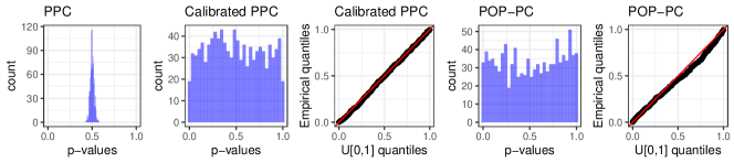
(a) Distribution of $p$-values when the data is Gaussian (Equation 18).

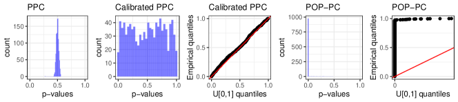
(b) Distribution of $p$-values when the data is Cauchy (Equation 19).

Figure 3: In the Gaussian mean example, the pop-pc detects model misspecification (i.e. when the data is actually Cauchy) while the ppc and calibrated ppc do not.

5 Empirical Study

We study population predictive checks on a regression model and a hierarchical model of documents.

• In the regression model study:

  1. We show empirically that the pop-pc detects overfitting when there is insuficient regularization. In contrast, the ppc, as well as the calibration suggestions of Robins et al., (2000) and Hjort et al., (2006), do not detect overfitting when there is insufficient regularization.

  2. We show empirically that the pop-pc $p$-values are approximately uniform when the model has sufficient regularization (i.e. the pop-pc is calibrated). In contrast, the ppc $p$-values are not calibrated.

• For the hierarchical model of documents:

  1. On synthetic data, we show empirically that the pop-pc $p$-values are approximately uniform when the data actually comes from the model (i.e. the pop-pc is calibrated).

  2. On a collection of documents from the New York Times, we show that the pop-pc detects model misfit due to overfitting, while the ppc does not.

5.1 Bayesian Ridge Regression

In this section, we return to the regression example in Section 2.1. We now compare the pop-pc with a variety of methods for Bayesian model criticism for a range of different values of the prior variance $c$.

In the large $c$ scenario, we expect that a posterior predictive check will not be able to detect the overfitting of the data. Moreover, as discussed in Section 4, we expect the calibration strategies of Robins et al., (2000) and Hjort et al., (2006) will also not detect this overfitting. In contrast, we expect that a population predictive check will be able to detect overfitting, and reject the model with large prior variance values. We also consider prior predictive checks (Box,, 1980).

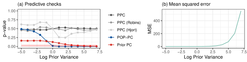
Figure 4: Bayesian ridge regression: pop-pc detects overfitting when there is little regularization (large $c$), while the ppc (including calibrated versions) does not. (a) average $p$-values over different $c$ from ppc, calibrated ppc s (Robins et al.,, 2000; Hjort et al.,, 2006), pop-pc and prior PC. (b) mean squared error of fitted model (Equation 13) over different values of $c$.

As anticipated, the ppc $p$-values are constant for all values of the regularization parameter, $c$; that is, the ppc cannot detect model misfit for large values of $c$ (Figure 4(b)). Moreover, the two calibrated ppc s (Robins et al.,, 2000; Hjort et al.,, 2006) also cannot detect this model misfit. Meanwhile, the pop-pc retains the model for small values of $c$. For large values of $c$, the pop-pc rejects the model as it overfits to the observed data. The prior predictive check exhibits similar behavior to the pop-pc, but it does not begin to reject the model until larger values of $c$.

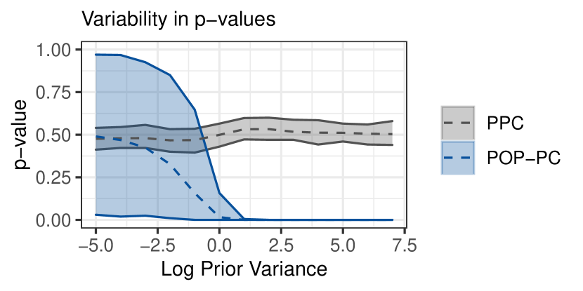
(a) pop-pc vs. ppc

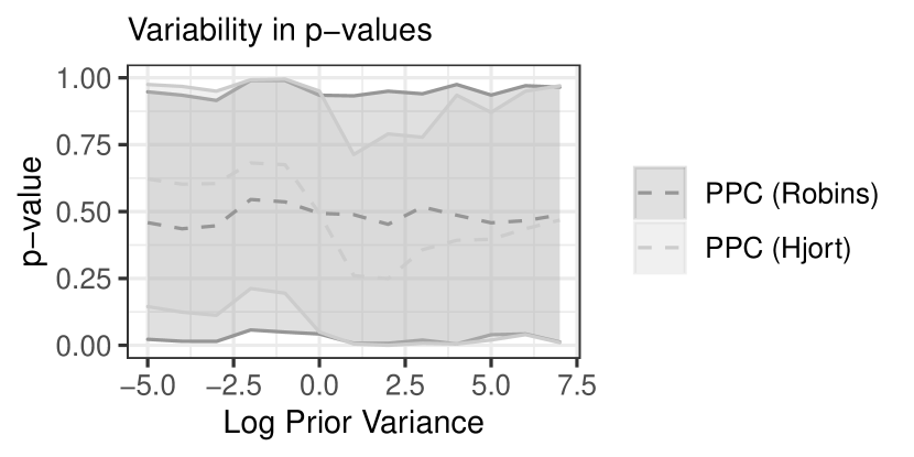
(b) Calibrated ppcs (Robins et al.,, 2000; Hjort et al.,, 2006)

Figure 5: Bayesian ridge regression: (a) When the model is not overfit, the pop-pc $p$-values are much more variable than ppc $p$-values, which concentrate around 0.5. When the model is overfit, pop-pc $p$-values detect this overfitting while ppc $p$-values do not. (b) Calibrated ppc $p$-values are much more variable than the ppc; however, the calibrated ppc does not detect overfitting for large $c$. For both (a) and (b), solid lines show 0.025 and 0.975 quantiles of $p$-values over $K=100$ replicates for different values of the regularization parameter $c$; dotted line shows mean.

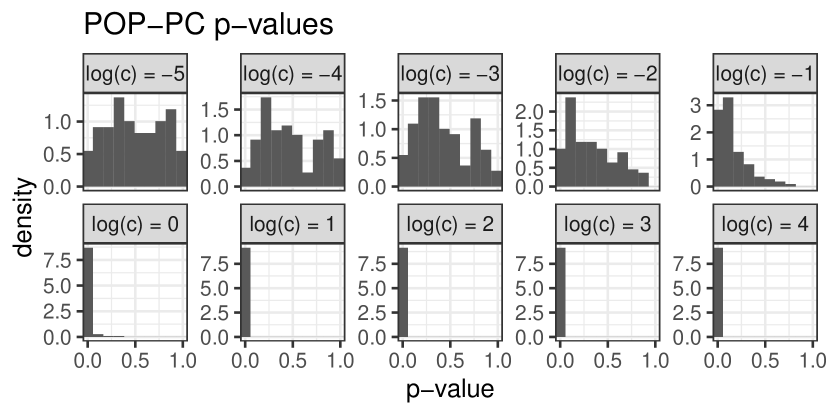
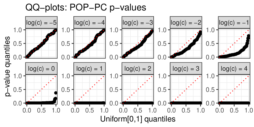
Figure 6: Bayesian ridge regression: pop-pc $p$-values are approximately uniform when there is no overfitting (small $c$); then, the pop-pc detects when there is overfitting (large $c$). Left: Histograms of pop-pc $p$-values. Right: QQ-plots comparing the quantiles of the pop-pc $p$-values with the quantiles of a uniform[0,1] random variable. Plots are over $K=100$ replications of the data.

We next consider the variability of the $p$-values from the predictive checks. As anticipated by the theoretical results of Robins et al., (2000), the ppc $p$-value is tightly concentrated around 0.5 for all values of $c$ (Figure 5(b)). Meanwhile, the empirical calibration procedures of Robins et al., (2000); Hjort et al., (2006) give $p$-values with greater variability around 0.5, as expected from the calibration process; however, they still do not reject the model for large $c$ (Figure 5(b)). In contrast, the pop-pc $p$-values show greater variability around 0.5 for small values of $c$ and then concentrate around 0 for large values of $c$ (Figure 5(a)).

The empirical distribution of the pop-pc $p$-values are displayed in Figure 6. The $p$-values are approximately uniform for small values of $c$. This provides empirical evidence for the calibration of pop-pc $p$-values with the $\chi^{2}$-diagnostic. For large values of $c$, the $p$-values concentrate around 0; that is, the pop-pc has high power to detect model misfit. Additional histograms and QQ-plots of the $p$-value distributions for all methods are in Appendix E of the Supplementary Material.

In theory, the pop-pc is calibrated for asymptotically normal diagnostic statistics (Theorem 1). In this regression example, the diagnostic statistic is $\chi^{2}$ distributed, not normal. Although our theory does not extend to this diagnostic, we showed empirically that the pop-pc has good calibration properties.

5.2 Topic Modeling

We next study pop-pcs on latent Dirichlet allocation (lda) (Blei et al.,, 2003), a hierarchical model of documents. We first apply LDA to synthetic data and show empirically the pop-pc has good calibration properties. We then apply LDA to a collection of documents from the New York Times and show that the pop-pc detects model misfit due to overfitting.

lda models documents as mixtures over latent topics, where each topic is a distribution over words. The $k$th topic is denoted by $\beta_{k}=\{\beta_{kv}\}_{v=1}^{V}$, where $V\in\mathbb{N}$ is the number of unique words in the corpus, and the number of topics ranges from $k=1,\dots,K$. The topics are drawn as:

$$\beta_{k}\sim\text{Dirichlet}(\alpha\mathbf{1}_{V}),\quad k=1,\dots,K,$$ (36)

where $\alpha\in\mathbb{R}^{+}$ is a hyperparameter.

For the $d$th document, the generative process is:

1. Draw the topic proportions $\theta_{d}\sim\text{Dirichlet}(\alpha\mathbf{1}_{K})$

2. For words $n=1,\dots,N_{d}$:

   1. Draw a topic $z_{dn}\sim\text{Multinomial}(\theta_{d})$

   2. Draw a word conditioned on the topic $w_{dn}\sim\text{Multinomial}(\beta_{z_{dn}})$

We set the Dirichlet hyperparameter to $\alpha=0.1$ on both the topics and the document proportions.

For the model check diagnostic, we will use the log-likelihood. For document $d$, the log-likelihood is:

$$\ell(\bm{w}_{d};\theta_{d},\bm{\beta})=\sum_{v=1}^{V}\left[\sum_{n=1}^{N_{d}}\mathbbm{1}(w_{dn}=v)\right]\log\left(\sum_{k=1}^{K}\beta_{kv}\theta_{dk}\right).$$ (37)

To calculate the ppc $p$-value, we first estimate the local per-document parameters, $\{\theta_{d}\}_{d=1}^{D}$, given the expectation of the global topics $\widehat{\bm{\beta}}=\mathbb{E}[\bm{\beta}|\bm{w}_{1:D}]$. Then, we draw replicates from the posterior predictive distribution and calculate the per-document ppc as:

$$\textrm{ppc}(\bm{w}_{d}^{\textrm{obs}}) =\frac{1}{R}\sum_{r=1}^{R}\mathbbm{1}[\ell(\bm{w}_{d,r}^{\textrm{rep}},\theta_{d,r},\widehat{\bm{\beta}})>\ell(\bm{w}_{d}^{\textrm{obs}},\theta_{d,r},\widehat{\bm{\beta}})],$$ (38)

where $$\quad(\bm{w}_{d,r}^{\textrm{rep}},\theta_{d,r})\sim p(\bm{w}_{d}^{\textrm{rep}}|\theta_{d},\widehat{\bm{\beta}})p(\theta_{d}|\bm{w}_{d}^{\textrm{obs}},\widehat{\bm{\beta}}).$$ (39)

Note that the topic vector $\bm{\beta}$ is fixed; we are checking the fit of the model based on the document topic proportions $\theta_{d}$.

To calculate the pop-pc $p$-value, we first split the set of documents in half: $\bm{w}_{d}=\{\bm{w}_{d}^{\textrm{obs}},\bm{w}_{d}^{\textrm{new}}\}_{d=1}^{D}$. Half of the document is used to infer the per-document local variable, $\theta_{d}$, and the other half is used to check the model:

$$\textrm{pop}(\bm{w}_{d}^{\textrm{obs}},\bm{w}_{d}^{\textrm{new}}) =\frac{1}{R}\sum_{r=1}^{R}\mathbbm{1}[\ell(\bm{w}_{d,r}^{\textrm{rep}},\theta_{d,r},\widehat{\bm{\beta}})>\ell(\bm{w}_{d}^{\textrm{new}},\theta_{d,r},\widehat{\bm{\beta}})],$$ (40)

where $$\quad(\bm{w}_{d,r}^{\textrm{rep}},\theta_{d,r})\sim p(\bm{w}_{d}^{\textrm{rep}}|\theta_{d},\widehat{\bm{\beta}})p(\theta_{d}|\bm{w}_{d}^{\textrm{obs}},\widehat{\bm{\beta}}).$$ (41)

5.3 Synthetic data

We investigate the distribution of pop-pc and ppc $p$-values when the data is drawn from the LDA generative process with $K=10$ topics and $V=2500$ vocabulary of unique words. The number of words (tokens) in each document is drawn as $N_{d}\sim\text{Poisson}(\xi)$ where $\xi=300$.

We draw $100,000$ documents and infer the topics $\beta$ using stochastic variational inference (Hoffman et al.,, 2013) with minibatches of size 100. Given the topics $\beta$, we then compare the ppc and pop-pc on a subset of documents of size $D=1,000$.

For each document, we calculate the ppc and pop-pc $p$-values using the log-likelihood diagnostic with $R=500$ replicates from the posterior predictive distribution. The pop-pc $p$-values are approximately uniformly distributed while the ppc $p$-values are left-skewed (Figure 7). This provides empirical evidence that the pop-pc is calibrated for the LDA log-likelihood diagnostic.

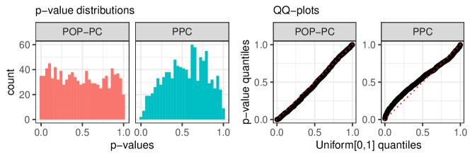
Figure 7: Simulated LDA data: when the model is true, pop-pc $p$-values are approximately uniform while ppc $p$-values are not. Left: Histograms of pop-pc and ppc $p$-values. Right: QQ-plots comparing the quantiles of the pop-pc and ppc $p$-values with the quantiles of a uniform[0,1] random variable.

5.4 New York Times

We consider a corpus of 100,000 news documents with a vocabulary size of 5,000 unique words from the New York Times. To infer the topics $\beta$, we implement stochastic variational inference (Hoffman et al.,, 2013) with minibatches of size 100. Given the topics $\beta$, we then compare the ppc and pop-pc on a subset of documents of size 1,000.

For each document, we calculate the ppc and pop-pc $p$-values using the log-likelihood diagnostic averaged over documents, where for each document we draw $R=500$ replicates from the posterior predictive distribution.

As the number of topics increases to $K=1,000$, the ppc $p$-value remains close to 0.5, and the negative log-likelihood is monotonically decreasing (Figure 8). At $K=1,000$, the number of topics is equal to the size of the vocabulary; at this stage, the model assigns each word to its own topic, memorizing the data. The pop-pc $p$-value detects this overfitting, and begins to reject the model past $K=200$ topics (Figure 8 left).

Note that when the number of topics is small, the pop-pc does not reject the model. A similar phenomenon was noted in Moran et al., (2022) for a Gaussian mixture model when the number of mixtures components is fewer than the truth. When the number of mixture components is too few, the entropy of the posterior predictive distribution increases to fit the data. The draws from this posterior distribution can be extreme relative to the true model, making it difficult to distinguish model misfit.

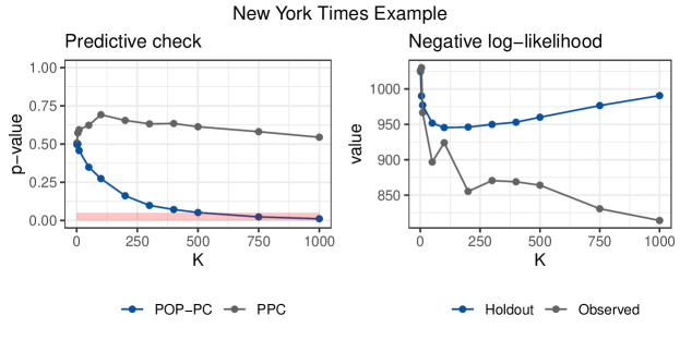
Figure 8: On the New York Times data, the pop-pc detects model overfitting, rejecting the model when the number of topics is large. In contrast, the ppc never rejects the model. Left: pop-pc and ppc $p$-values for different values of topics $K$. Right: Negative log-likelihood on observed and holdout data over different values of topics $K$.

6 Discussion

We developed population predictive checks (pop-pcs), a diagnostic tool that brings together Bayesian methods for model checking with frequentist estimation of goodness of fit. The pop-pc assesses a Bayesian model by comparing samples from the posterior predictive to a sample from the population distribution, which in practice is a heldout dataset. We proved that the pop-pc is calibrated for a class of asymptotically normal diagnostic functions and empirically show its calibration for other diagnostics. We revisited the “double use of the data” issue of posterior predictive checks (ppcs) and highlighted that while post-hoc procedures can be used to calibrate the ppc, post-hoc calibration does not provide power to detect model misfit. Finally, we demonstrated the utility of pop-pcs with Bayesian linear regression models and on probabilistic topic models of documents.

There are several areas for further research. For hierarchical models of grouped data, Marshall and Spiegelhalter, (2003) define mixed predictive checks, where the reference distribution combines the prior for the group-specific latent variables with the posterior for latent variables shared across groups. This approach mitigates the overconfidence of a ppc, but there are no guarantees; a mixed predictive check can still be overconfident if the influence of the posterior becomes too large. To avoid such overconfidence, Bayarri and Castellanos, (2007) extends the checks of Bayarri and Berger, (2000) to hierarchical models. How to extend the pop-pc to these situations is one avenue of further research.

Generalizing beyond hierarchical models, researchers have studied how to check individual components of a probabilistic model, i.e., individual nodes in a directed graphical model. O’Hagan, (2003) proposes some of the earlier ideas along these lines, though in a way that uses the data twice and leads to overconfident checks. To correct for such overconfidence, his predictive checks for individual components of a model have been extended, often by using data splitting (Marshall and Spiegelhalter,, 2007; Bayarri and Castellanos,, 2007; Dahl et al.,, 2007; Gåsemyr and Natvig,, 2009; Presanis et al.,, 2013). Again the pop-pc proposed here could be extended to these settings.

Appendix A Proofs

A.1 Proof of calibration of the population predictive check

In this section, we prove Theorem 1. Recall that we assume the diagnostic $d(\bm{y})$ is asymptotically normal with asymptotic mean $\nu(\theta)$ and asymptotic variance $\sigma^{2}(\theta)$, under the null hypothesis that the density of $\bm{y}$ is $f(\bm{y};\theta)$:

$$n^{1/2}\left[\frac{d(\bm{y})-\nu(\theta)}{\sigma(\theta)}\right]\leadsto N(0,1),$$ (42)

where $\leadsto$ denotes convergence in distribution.

Notation. We let $\mathrm{p}(\theta|\bm{y})$ denote the posterior distribution of $\theta$. We use $\lVert\cdot\rVert$ to denote the total variation distance between two distributions $P$ and $Q$. The Fisher information is

$$I(\theta)=\lim_{n\to\infty}n^{-1}\mathbb{E}_{\theta}\left[-\partial^{2}\log f(\bm{y};\theta)/\partial\theta\partial\theta^{\prime}\right].$$ (43)

We use the notation $y_{n}=O_{p}(a_{n})$ as $n\to\infty$ to mean $y_{n}/a_{n}$ is stochastically bounded: for any $\varepsilon>0$, there exists finite $M>0$ and $N>0$ such that

$$\mathrm{p}(|y_{n}/a_{n}|>M)<\varepsilon,\quad\forall n>N.$$ (44)

We use $\phi(\theta;\mu,\Sigma)$ to denote the density of a $N(\mu,\Sigma)$ random variable.

Regularity conditions.

1. The asymptotic mean $\nu$ is continuously differentiable in a neighborhood of $(0,\theta)$, with partial derivatives converging to limit:

   $$\dot{\nu}(\theta_{0}) =\lim_{n\to\infty}\partial\nu_{n}(0,\theta)/\partial\theta\big{|}_{\theta=\theta_{0}}.$$ (45)

2. For some $p$-vector-valued function $\theta(\bm{y})$ on the sample space, we assume

   $$\lVert\mathrm{p}(\cdot|\bm{y})-N(\theta(\bm{y}),I^{-1}(\theta_{0})/n)\rVert\stackrel{{\scriptstyle P_{\theta_{0}}}}{{\to}}0$$ (46)

   and

   $$n^{1/2}(\theta(\bm{y})-\theta_{0})=O_{P_{\theta_{0}}}(1).$$ (47)

Proof of Theorem 1.

Our proof technique follows that of Robins et al., (2000) for their proof of Theorem 3.

The pop-pc $p$-value is:

$$p(\bm{y}^{\mathrm{obs}},\bm{y}^{\mathrm{new}})=\int_{\Theta}\mathrm{p}(d(\bm{y}^{\mathrm{rep}})>d(\bm{y}^{\mathrm{new}})|\bm{y}^{\mathrm{new}},\theta)\mathrm{p}(\theta|\bm{y}^{\mathrm{obs}})d\theta$$ (48)

Consider:

$$d(\bm{y}^{\mathrm{rep}}) >d(\bm{y}^{\mathrm{new}})$$ (49)

$$\text{Then,}\qquad\qquad\sqrt{n}[d(\bm{y}^{\mathrm{rep}})-\nu(\theta)] >\sqrt{n}[d(\bm{y}^{\mathrm{new}})-\nu(\theta_{0})-(\nu(\theta)-\nu(\theta_{0}))].$$ (50)

Consider the LHS of Equation 50. By Equation 42, we have that, conditional on $\theta$,

$$\sqrt{n}[d(\bm{y}^{\mathrm{rep}})-\nu(\theta)]\sim N(0,\sigma^{2}(\theta_{0})).$$

Consider now the RHS of Equation 50. The first term $\sqrt{n}[d(\bm{y}^{\mathrm{new}})-\nu(\theta_{0})]$ is fixed, conditional on $\bm{y}^{\mathrm{new}}$. For the second term, we use a Taylor expansion to obtain:

$$\nu(\theta)-\nu(\theta_{0})\approx\dot{\nu}(\theta_{0})(\theta-\theta_{0}).$$ (51)

Then by Equation 46, given $\bm{y}^{\mathrm{obs}}$, the second term is approximately distributed as

$$N(\dot{\nu}(\theta_{0})^{T}n^{1/2}(\theta(\bm{y}^{\mathrm{obs}})-\theta_{0}),\dot{\nu}(\theta_{0})^{T}I^{-1}(\theta_{0})\dot{\nu}(\theta_{0})).$$ (52)

(Note this step using Equation 46 helps resolve the potentially difficult integral over $\mathrm{p}(\theta|\bm{y}^{\mathrm{obs}})$.)

Then, the conditional probability, given $\bm{y}^{\mathrm{obs}}$ and $\bm{y}^{\mathrm{new}}$, of $d(\bm{y}^{\mathrm{rep}})>d(\bm{y}^{\mathrm{new}})$ is approximately

$$\mathrm{p}(W>0|\bm{y}^{\mathrm{obs}},\bm{y}^{\mathrm{new}}),$$ (53)

where $W$ is a Gaussian random variable with

$$\mathbb{E}[W|\bm{y}^{\mathrm{obs}},\bm{y}^{\mathrm{new}}] =n^{1/2}\dot{\nu}(\theta_{0})^{T}(\theta(\bm{y}^{\mathrm{obs}})-\theta_{0})-n^{1/2}[d(\bm{y}^{\mathrm{new}})-\nu(\theta_{0})],$$ (54)

$$\text{Var}(W|\bm{y}^{\mathrm{obs}},\bm{y}^{\mathrm{new}}) =\sigma^{2}(\theta_{0})+\dot{\nu}(\theta_{0})^{T}I^{-1}(\theta_{0})\dot{\nu}(\theta_{0}).$$ (55)

Then, the pop-pc $p$-value is

$$p(\bm{y}^{\mathrm{obs}},\bm{y}^{\mathrm{new}}) =1-\Phi\left(\frac{n^{1/2}\dot{\nu}(\theta_{0})^{T}(\theta(\bm{y}^{\mathrm{obs}})-\theta_{0})-n^{1/2}[d(\bm{y}^{\mathrm{new}})-\nu(\theta_{0})]}{\sqrt{\sigma^{2}(\theta_{0})+\dot{\nu}(\theta)^{T}I^{-1}(\theta_{0})\dot{\nu}(\theta)}}\right)+o_{P_{0}}(1),$$ (56)

where we have used Equation 46.

Now, we consider the distribution of the pop-pc $p$-value over the distributions of $\bm{y}^{\mathrm{obs}}$ and $\bm{y}^{\mathrm{new}}$.

By Equation 47, we have that the posterior mean converges to the true $\theta_{0}$:

$$\sqrt{n}\dot{\nu}(\theta_{0})^{T}(\theta(\bm{y}^{\mathrm{obs}})-\theta_{0})\leadsto N(0,\dot{\nu}(\theta_{0})^{T}I^{-1}(\theta_{0})\dot{\nu}(\theta_{0})).$$ (57)

Independently, $n^{1/2}[d(\bm{y}^{\mathrm{new}})-\nu(\theta_{0})]$ converges to a $N(0,\sigma^{2}(\theta_{0}))$ distribution.

Hence, the pop-pc $p$-value is:

$$p(\bm{y}^{\mathrm{obs}},\bm{y}^{\mathrm{new}}) =1-\Phi\left(Q\right)+o_{P_{0}}(1),$$ (58)

where $Q\sim N(0,1)$.

This concludes the proof.

Appendix B Note on previous version of this paper

The previous version of this paper, Ranganath and Blei, (2019), proposed a different definition for the pop-pc (population predictive check, version 1 (pop-pc-v1)). The pop-pc-v1 treated $\bm{y}^{\mathrm{new}}$ as random; in the current population predictive check, $\bm{y}^{\mathrm{new}}$ is fixed. Treating $\bm{y}^{\mathrm{new}}$ as fixed results in a calibrated check, while treating $\bm{y}^{\mathrm{new}}$ as random does not. For completeness, we include the previous definition of the pop-pc below.

Definition 2 (Population predictive check (Version 1, 2019))

Consider observed data $\bm{y}^{\mathrm{obs}}$, its posterior predictive distribution $\mathrm{p}(\bm{y}^{\mathrm{rep}}\,|\,\bm{y}^{\mathrm{obs}})$, and a diagnostic statistic $d(\bm{y})$. Suppose we have $\bm{y}^{\mathrm{new}}$ drawn from the population distribution of the data. The population predictive check as a $p$-value is:

$$p_{\mathrm{pop-v1}}=\mathrm{p}(d(\bm{y}^{\mathrm{rep}})\geq d(\bm{y}^{\mathrm{new}})\,|\,\bm{y}^{\mathrm{obs}}),\quad\bm{y}^{\mathrm{new}}\sim F$$ (59)

where $\bm{y}^{\mathrm{rep}}\sim\mathrm{p}(\bm{y}^{\mathrm{rep}}\,|\,\bm{y}^{\mathrm{obs}})$.

To illustrate the issue with treating $\bm{y}^{\mathrm{new}}$ as random, we again consider the mean example in Section 4. Suppose we observe data $\bm{y}^{\mathrm{obs}}=\{y_{i}\}_{i=1}^{n}$ drawn from a Gaussian with known variance parameter:

$$y_{i}\sim N(\mu,\sigma^{2}),$$ (60)

for some $\mu\in\mathbb{R}$ and fixed $\sigma^{2}$. For a prior on $\mu$, we take $\mu\sim N(\mu_{0},\sigma_{0}^{2})$ with fixed hyperparameters $\mu_{0}\in\mathbb{R},\sigma_{0}^{2}\in\mathbb{R}^{+}$.

In this case, the posterior predictive distribution is

$$\overline{\bm{y}}^{\mathrm{rep}}|\overline{\bm{y}}^{\mathrm{obs}}\sim N\left(\rho_{n}\overline{\bm{y}}^{\mathrm{obs}}+(1-\rho_{n})\mu_{0},\left(1+\rho_{n}\right)\frac{\sigma^{2}}{n}\right).$$ (61)

As $n\to\infty$, $\overline{\bm{y}}^{\mathrm{rep}}|\overline{\bm{y}}^{\mathrm{obs}}$ is centered around $\overline{\bm{y}}^{\mathrm{obs}}$. This is different from the distribution of $\bm{y}^{\mathrm{new}}$, which is the population distribution: $\overline{\bm{y}}^{\mathrm{new}}\sim N(\mu,\sigma^{2})$ (see Figure 9). Consequently, the pop-pc-v1 is not calibrated. We demonstrate this lack of calibration theoretically below.

Consider the distribution of pop-pc-v1 when Equation 60 holds:

$$\mathrm{p}(d(\bm{y}^{\mathrm{rep}})>d(\bm{y}^{\mathrm{new}})|\bm{y}^{\mathrm{obs}})=\mathrm{p}(D>0|\bm{y}^{\mathrm{obs}}),$$ (62)

where $D=d(\bm{y}^{\mathrm{rep}})-d(\bm{y}^{\mathrm{new}})$ is a Gaussian random variable with

$$\mathrm{E}[D|\bm{y}^{\mathrm{obs}}]=\rho_{n}\overline{\bm{y}}^{\mathrm{obs}}+(1-\rho_{n})\mu_{0}-{\mu},\quad Var(D)=\left(2+\frac{\rho_{n}}{n}\right)\frac{\sigma^{2}}{n}.$$ (63)

The pop-pc-v1 is then:

$$\mathrm{p}(D>0|\bm{y}^{\mathrm{obs}})=1-\Phi\left(\frac{{\mu}-\rho_{n}\overline{\bm{y}}^{\mathrm{obs}}-(1-\rho_{n})\mu_{0}}{\sqrt{(2+\rho_{n})\sigma^{2}/n}}\right)$$ (64)

Now, if the observed data has the same distribution as the new data, we have $\overline{\bm{y}}^{\mathrm{obs}}\sim N({\mu},\sigma^{2}/n)$. Then, for large $n$, the pop-pc $p$-value (Version 1, 2019) is:

$$\mathrm{p}(D>0|\bm{y}^{\mathrm{obs}})\to 1-\Phi\left(Z/\sqrt{3}\right),\quad\text{where }Z\sim N(0,1).$$ (65)

Consequently, the pop-pc-v1 is not calibrated.

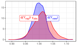
Figure 9: The distribution of $d(\bm{y}^{\mathrm{new}})=\overline{\bm{y}}^{\mathrm{new}}$ is not equal to the distribution of $d(\bm{y}^{\mathrm{rep}})=\overline{\bm{y}}^{\mathrm{rep}}$. (Data drawn as $y_{i}\sim N(1,1)$, $i=1,\dots,2000$).

The updated definition of the pop-pc in Definition 1 does not have this calibration issue. Intuitively, this is because a fixed $\bm{y}^{\mathrm{new}}$ is on average as far from the true mean as the fixed $\bm{y}^{\mathrm{obs}}$.

For the more general case of asymptotically normal diagnostic functions, we also prove the pop-pc-v1 is not uniformly distributed.

Theorem 2

We assume Equation 16 holds, in addition to regularity conditions detailed in Section A.1. Under the distribution $f(\bm{y};\theta_{0})$, the pop-pc-v1 $p$-value can be written as:

$$p_{\mathrm{pop-v1}}(\bm{y})=1-\Phi(Q)+o_{P}(1),\text{ where }Q\sim N\left(0,\frac{\dot{\nu}_{\theta}(\theta_{0})^{T}I^{-1}(\theta_{0})\dot{\nu}_{\theta}(\theta_{0})}{2\sigma^{2}(\theta_{0})+\dot{\nu}_{\theta}(\theta_{0})^{T}I^{-1}(\theta_{0})\dot{\nu}_{\theta}(\theta_{0})}\right),$$ (66)

where $o_{P}(1)$ denotes a random variable converging to zero in probability, $\Phi$ is the standard normal cdf, and $Q\sim N(0,1)$.

Consequently, the pop-pc-v1 is not calibrated.

Proof of Theorem 2.

The pop-pc-v1 $p$-value is:

$$p(\bm{y}^{\mathrm{obs}})=\int_{\Theta}\mathrm{p}(d(\bm{y}^{\mathrm{rep}})>d(\bm{y}^{\mathrm{new}})|\theta)\mathrm{p}(\theta|\bm{y}^{\mathrm{obs}})\mathrm{p}(\bm{y}^{\mathrm{new}}|\theta_{0})d\theta$$ (67)

Consider:

$$d(\bm{y}^{\mathrm{rep}}) >d(\bm{y}^{\mathrm{new}})$$ (68)

$$\text{Then,}\qquad\qquad\sqrt{n}[d(\bm{y}^{\mathrm{rep}})-\nu(\theta)] >\sqrt{n}[d(\bm{y}^{\mathrm{new}})-\nu(\theta_{0})-(\nu(\theta)-\nu(\theta_{0}))].$$ (69)

Consider the LHS of Equation 69. By Equation 42, we have

$$\sqrt{n}[d(\bm{y}^{\mathrm{rep}})-\nu(\theta)]\sim N(0,\sigma^{2}(\theta_{0})).$$

Consider now the RHS of Equation 69. The first term is distributed as:

$$\sqrt{n}[d(\bm{y}^{\mathrm{new}})-\nu(\theta_{0})]\sim N(0,\sigma^{2}(\theta_{0})).$$ (70)

For the second term, we use a Taylor expansion to obtain:

$$\nu(\theta)-\nu(\theta_{0})\approx\dot{\nu}(\theta_{0})(\theta-\theta_{0}).$$ (71)

Then by Equation 46, given $\bm{y}^{\mathrm{obs}}$, the second term is approximately distributed as

$$N(\dot{\nu}(\theta_{0})^{T}n^{1/2}(\theta(\bm{y}^{\mathrm{obs}})-\theta_{0}),\dot{\nu}(\theta_{0})^{T}I^{-1}(\theta_{0})\dot{\nu}(\theta_{0})).$$ (72)

(Note this step using Equation 46 helps resolve the potentially difficult integral over $\mathrm{p}(\theta|\bm{y}^{\mathrm{obs}})$.)

Then, the conditional probability, given $\bm{y}^{\mathrm{obs}}$, of $d(\bm{y}^{\mathrm{rep}})>d(\bm{y}^{\mathrm{new}})$ is approximately

$$\mathrm{p}(W>0|\bm{y}^{\mathrm{obs}}),$$ (73)

where $W$ is a Gaussian random variable with

$$\mathbb{E}[W|\bm{y}^{\mathrm{obs}}] =n^{1/2}\dot{\nu}(\theta_{0})^{T}(\theta(\bm{y}^{\mathrm{obs}})-\theta_{0}),$$ (74)

$$\text{Var}(W|\bm{y}^{\mathrm{obs}}) =2\sigma^{2}(\theta_{0})+\dot{\nu}(\theta_{0})^{T}I^{-1}(\theta_{0})\dot{\nu}(\theta_{0}).$$ (75)

Then, the pop-pc-v1 $p$-value is

$$p(\bm{y}^{\mathrm{obs}}) =1-\Phi\left(\frac{n^{1/2}\dot{\nu}(\theta_{0})^{T}(\theta(\bm{y}^{\mathrm{obs}})-\theta_{0})}{\sqrt{2\sigma^{2}(\theta_{0})+\dot{\nu}(\theta)^{T}I^{-1}(\theta_{0})\dot{\nu}(\theta)}}\right)+o_{P_{0}}(1),$$ (76)

where we have used Equation 46.

Now, we consider the distribution of the pop-pc-v1 $p$-value over the distribution of $\bm{y}^{\mathrm{obs}}$.

By Equation 47, we have that the posterior mean converges to the true $\theta_{0}$:

$$\sqrt{n}\dot{\nu}(\theta_{0})^{T}(\theta(\bm{y}^{\mathrm{obs}})-\theta_{0})\leadsto N(0,\dot{\nu}(\theta_{0})^{T}I^{-1}(\theta_{0})\dot{\nu}(\theta_{0})).$$ (77)

Hence, the pop-pc-v1 $p$-value is:

$$p(\bm{y}^{\mathrm{obs}}) =1-\Phi\left(Q\right)+o_{P_{0}}(1),$$ (78)

where $Q$ is a Gaussian random variable with mean $0$ and variance

$$\text{Var}(Q)=\frac{\dot{\nu}(\theta_{0})^{T}I^{-1}(\theta_{0})\dot{\nu}(\theta_{0})}{2\sigma^{2}(\theta_{0})+\dot{\nu}(\theta_{0})^{T}I^{-1}(\theta)\dot{\nu}(\theta_{0})}.$$ (79)

This concludes the proof.

Appendix C Details for Section 4

Suppose we observe data $\bm{y}=\{y_{i}\}_{i=1}^{n},y_{i}\sim N(\mu,\sigma^{2})$ where $\sigma^{2}$ is known. The prior is taken to be $\mu\sim N(\mu_{0},\sigma_{0}^{2})$.

We consider the posterior predictive $p$-value with diagnostic $d(\bm{y})=\overline{\bm{y}}$. The posterior predictive distribution of $\overline{\bm{y}}^{\mathrm{rep}}$ is:

$$\overline{\bm{y}}^{\mathrm{rep}}|\overline{\bm{y}}^{\mathrm{obs}} =\int\mathrm{p}(\overline{\bm{y}}^{\mathrm{rep}}|\theta)\mathrm{p}(\theta|\overline{\bm{y}}^{\mathrm{obs}})d\theta$$ (80)

$$\sim N\left(\rho_{n}\overline{\bm{y}}^{\mathrm{obs}}+(1-\rho_{n})\mu_{0},\left(1+\rho_{n}\right)\frac{\sigma^{2}}{n}\right)$$ (81)

where $\rho_{n}=n\sigma_{0}^{2}/(n\sigma_{0}^{2}+\sigma^{2})$.

Then, the posterior predictive $p$-value is:

$$\mathrm{p}(d(\bm{y}_{rep})>d(\bm{y}^{\mathrm{obs}})|\bm{y}^{\mathrm{obs}})) =1-\Phi\left(\frac{\overline{\bm{y}}^{\mathrm{obs}}-\rho_{n}\overline{\bm{y}}^{\mathrm{obs}}-(1-\rho_{n})\mu_{0}}{\sqrt{(1+\rho_{n})\sigma^{2}/n}}\right).$$ (82)

Appendix D Discussion of the partial predictive check

An alternative method to obtain calibrated $p$-values is the partial predictive check of Bayarri and Berger, (2000). The partial PC achieves calibration by calculating a conditional posterior predictive that is independent of the diagnostic. However, when the diagnostic includes the sufficient statistics of the model, the partial predictive check essentially becomes a prior predictive check. To illustrate this point, consider the partial predictive check for the test in Section 4. The partial predictive check uses the following predictive distribution:

$$\mathrm{p}(\bm{y}^{\mathrm{rep}}|\mu)\mathrm{p}(\mu|\bm{y}^{\mathrm{obs}}\backslash d(\bm{y}^{\mathrm{obs}})),\quad\text{where}\quad\mathrm{p}(\mu|\bm{y}^{\mathrm{obs}}\backslash d(\bm{y}^{\mathrm{obs}}))\propto\frac{\mathrm{p}(\bm{y}^{\mathrm{obs}}|\mu)\mathrm{p}(\mu)}{\mathrm{p}(d(\bm{y}^{\mathrm{obs}})|\mu)}.$$ (83)

In this example, $\mathrm{p}(\mu|\bm{y}^{\mathrm{obs}}\backslash\overline{\bm{y}}^{\mathrm{obs}})$ is simply the prior on $\mu$, as we are removing the influence of the sufficient statistic, $\overline{\bm{y}}^{\mathrm{obs}}$. Then, the distribution of the partial posterior predictive is

$$\overline{\bm{y}}^{\mathrm{rep}}|\bm{y}^{\mathrm{obs}}\backslash d(\bm{y}^{\mathrm{obs}})\sim N\left(\mu_{0},(\sigma_{0}^{2}+\sigma^{2})/n\right).$$ (84)

The partial predictive $p$-value is then:

$$\mathrm{p}(d(\bm{y}^{\mathrm{rep}})>d(\bm{y}^{\mathrm{obs}})|\bm{y}^{\mathrm{obs}}\backslash\overline{\bm{y}}^{\mathrm{obs}})=1-\Phi\left(\frac{\overline{\bm{y}}^{\mathrm{obs}}-\mu_{0}}{\sqrt{(\sigma_{0}^{2}+\sigma^{2})/n}}\right).$$ (85)

This is the prior predictive $p$-value. That is, if the diagnostic is the only sufficient statistic, the partial predictive $p$-value coincides with the prior predictive $p$-value, which is not calibrated. This does not contradict Robins et al., (2000); Bayarri and Berger, (2000), however, who prove the partial predictive check is calibrated under certain assumptions. One of these assumptions is that the parameters of the predictive distribution converge to the MLE, which is not the case here.

However, the partial posterior check is similar to the pop-pc when the partial diagnostic is defined to use a subset of the data. In the above example, we could choose $d(\bm{y}^{\mathrm{obs}})=1/(n/2)\sum_{i=1}^{n/2}y_{i}^{\mathrm{obs}}\eqqcolon\overline{\bm{y}}^{\mathrm{obs}}_{1:n/2}$ In this case, the conditional posterior is:

$$\mathrm{p}(\mu|\bm{y}^{\mathrm{obs}}\backslash d(\bm{y}^{\mathrm{obs}})) \propto\frac{\exp\left\{-\frac{1}{2}\sum_{i=1}^{n}\left[y_{i}^{\mathrm{obs}}-\mu\right]^{2}\right\}}{\exp\left\{-\frac{n}{4}\left[\overline{\bm{y}}_{1:n/2}-\mu\right]^{2}\right\}}\mathrm{p}(\mu)$$ (86)

$$\propto\prod_{i=n/2+1}^{n}\mathrm{p}(y^{\mathrm{obs}}_{i}|\mu)\mathrm{p}(\mu).$$ (87)

For this diagnostic, the partial posterior check is equivalent to the pop-pc.

In certain cases, the partial posterior check with a data-split diagnostic may be more efficient in its use of the data than pop-pc. This is because the pop-pc will always use a subset of the data for posterior inference. A partial predictive check meanwhile may only remove a sufficient statistic of this subset of the data. Despite this, the partial predictive check can be difficult to calculate, and requires re-calculation for each diagnostic function. Meanwhile, a pop-pc is simple to implement, and the inferred posterior can be used to check many different diagnostic functions.

Appendix E Additional details for Section 5

In this section, we provide additional plots for the regression study in Section 5.1.

• Figure 10 shows the empirical distribution of ppc $p$-values. The $p$-values are concentrated around 0.5 for all values of $c$.

• Figure 11 shows the empirical distribution of ppc $p$-values calibrated following Robins et al., (2000). While the $p$-values are uniform, they show a similar distribution for all values of $c$ and so are unable to detect model misfit.

• Figure 12 shows the empirical distribution of cppp $p$-values (Hjort et al.,, 2006). The cppp $p$-values do not detect model misfit for large $c$.

• Figure 6 shows the empirical distribution of the pop-pc $p$-values. For small values of $c$, the pop-pc $p$-values are approximately uniform. For large values of $c$, the pop-pc $p$-values concentrate around 0 (i.e. the pop-pc will always reject the model when there is insufficient regularization).

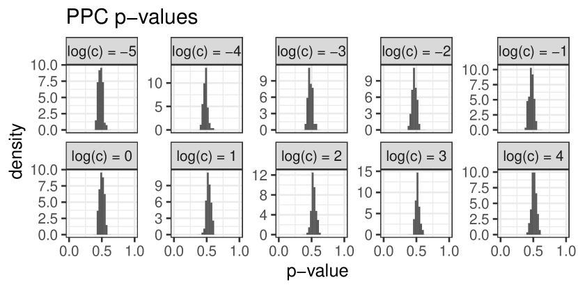
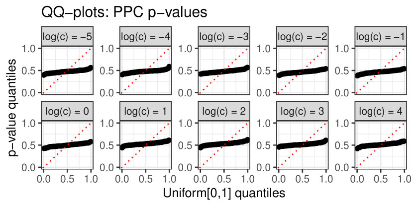
Figure 10: ppc $p$-values are concentrated around 0.5 for all values of the regularization parameter $c$. Left: Histograms of ppc $p$-values. Right: QQ-plots comparing the quantiles of the ppc $p$-values with the quantiles of a uniform[0,1] random variable.

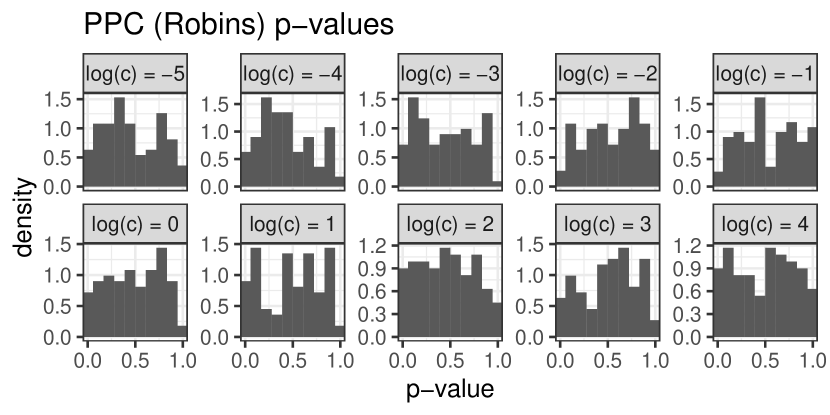
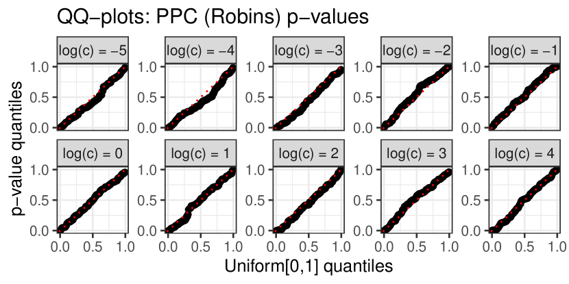
Figure 11: Calibrated ppc $p$-values (Robins et al.,, 2000) are approximately uniformly distributed but they do not detect overfitting for large values of the regularization parameter $c$. Left: Histograms of calibrated ppc $p$-values. Right: QQ-plots comparing the quantiles of the calibrated ppc $p$-values with the quantiles of a uniform[0,1] random variable. Plots are over $K=100$ replications of the data.

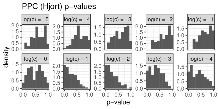
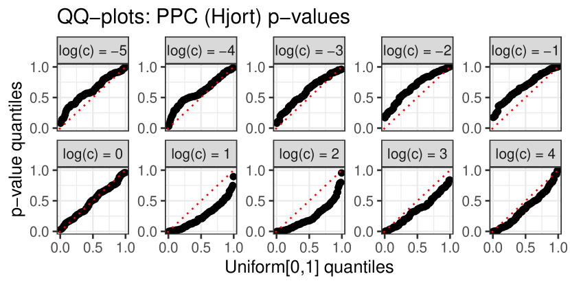
Figure 12: Calibrated cppp $p$-values (Hjort et al.,, 2006) do not detect overfitting for large values of the regularization parameter $c$. Left: Histograms of cppp $p$-values. Right: QQ-plots comparing the quantiles of the cppp $p$-values with the quantiles of a uniform[0,1] random variable. Plots are over $K=100$ replications of the data.

References

- Bayarri and Berger, (2000) Bayarri, M. and Berger, J. (2000). P-values for composite null models. Journal of the American Statistical Association, 95(452):1127–1142.
- Bayarri and Castellanos, (2007) Bayarri, M. and Castellanos, M. (2007). Bayesian checking of the second levels of hierarchical models. Statistical Science, 22:322–343.