Evolution of Spacelike Curves and Special Timelike Ruled Surfaces in the Minkowski Space

Abstract

In this paper, we get the time evolution equations of the curvature and torsion of the evolving spacelike curves in the Minkowski space. Also, we give inextensible evolutions of timelike ruled surfaces that are produced by the timelike normal and spacelike binormal vector fields of spacelike curve and derive the necessary conditions for an inelastic surface evolution. Then, we compute the coefficients of the first and second fundamental forms, the Gauss and mean curvatures for timelike special ruled surfaces. As a result, we give applications of the evolution equations for the curvatures of the curve in terms of the velocities and get the exact solutions for these new equations.

${\dagger}$ Department of Mathematics Education and RINS

Gyeongsang National University

Jinju 52828, Republic of Korea

E-mail address: dwyoon@gnu.ac.kr

${\ddagger}$, $\S$ Department of Mathematics

Fırat University

23119 Elazig, Turkey

E-mail address: zuhal2387@yahoo.com.tr, ebrucavlak@hotmail.com

1 Introduction

The time evolution of a curve or a surface is generated by flows, in particular inextensible flows of a curve or a surface. The flow of a curve or a surface is said to be inextensible if its arclength is preserved or the intrinsic curvature is preserved, respectively. Physically, the inextensible curve flows lead to motions in which no strain energy is induced. Also, the evolutions of curves have many important applications of physics as magnetic spin chains and vortex filaments [4, 10, 13].

The problems of how to get the evolution of the curves or surfaces in time is of deep interest and have been studied in different spaces by many researchers. Kwon et al. derived the corresponding equations for inextensible flows of developable surfaces, [12]. Hussien et al. obtained the evolutions of the special surfaces rely on the evolutions of their directrices, [11]. Recently, many authors have studied geometric flow problems on the curves or surfaces [1, 2, 3, 5, 9, 14, 21, 22].

In this study, we get the evolution of curves via the velocities of the moving frame in Minkowski space. We also classify the special timelike ruled surfaces on the evolving spacelike curve where the generator is the timelike principal and spacelike binormal vectors to the spacelike curves on the timelike surfaces. We give the necessary conditions for the inelastic special ruled surface evolutions and compute the gauss and mean curvatures for them. Then, we obtain a pair of coupled nonlinear partial differential equations governing the time evolution of the curvatures of the evolving spacelike curve in Minkowski space. We give the new geometric models of the evolution equations for curvatures from the main equation in Minkowski space and get the exact solutions for them and show the moving curve for these solutions. From these exact solutions, we derive two types of nonlinear traveling solitary wave, which are kink and bell-shaped solitary waves. The kink solitary wave appears balance between nonlinearity and dissipation supports known the nonlinear wave of stable shape. The bell-shaped solitary wave appears in consequence of the balance between nonlinearity and dispersion. Also, the bell-shaped wave improve to evaluate the dynamic modulus [7, 19].

2 Preliminaries

The 3-dimensional Minkowski space $E_{1}^{3}$ is the real vector space $E^{3}$ provided with the Lorentzian inner product given

$$\left\langle a,b\right\rangle=a_{1}b_{1}+a_{2}b_{2}-a_{3}b_{3},$$

with $a=(a_{1},a_{2},a_{3})$ and $b=(b_{1},b_{2},b_{3})$.

A vector $a\in E_{1}^{3}$ is said to be a spacelike vector when $\left\langle a,a\right\rangle>0$ or $a=0$. It is said to be a timelike and a null (light-like) vector in case of $\left\langle a,a\right\rangle<0$, and $\left\langle a,a\right\rangle=0$ for $a\neq 0$, respectively. Similarly, a curve is said to be spacelike, if its velocity vector is spacelike. For furthermore information, we refer to [16].

Let $r=r(s)$ be a spacelike curve in 3-dimensional Minkowski space $E_{1}^{3}$. Then Frenet formulas are given by

$$\left\{\begin{array}[]{c}T_{s}=\kappa N\\ N_{s}=\kappa T+\tau B\\ B_{s}=\tau N\end{array}\right.,$$ (2.1)

where $T=r_{s},$ $N$ and $B$ are called the vectors of the unit spacelike tangent, timelike principal normal and spacelike binormal of $r(s)$, respectively. Also $\kappa$ and $\tau$ are geometric parameters that represent, respectively, the curvature and torsion of $r(s),$ [20]. Through this paper, the subscripts describe partial derivatives.

We also know that a curve is uniquely given by two scalar quantities, so-called curvature and torsion.

If $r(s)$ moves with time $t,$ then (2.1) is becoming functions of both $s$ and $t$. We can give the evolution equations of $\{T,N,B\}$ quite generally, in a form similar to (2.1) as following [17]

$$\left\{\begin{array}[]{c}T_{t}=\alpha N-\beta B\\ N_{t}=\alpha T+\gamma B\\ B_{t}=\beta T+\gamma N\end{array}\right..$$ (2.2)

Clearly, $\alpha,\beta$ and $\gamma$ (which are the velocities of the moving frame) detect the motion of the $\alpha$.

Let $x=x(s,t)$ be a surface parametrization in $E_{1}^{3}$. Then, the vectors $x_{s}$ and $x_{t}$ are tangential to $M$ at $p$. Let $U$ be the standard unit normal vector field on a surface defined by

$$U=\frac{x_{s}\wedge x_{t}}{\left\|x_{s}\wedge x_{t}\right\|}.$$ (2.3)

Then the first and the second fundamental forms of a surface are given by [6, 15], respectively,

$$I = Eds^{2}+2Fdsdt+Gdt^{2},$$

$$II = eds^{2}+2fdsdt+gdt^{2},$$

where

$$E = \left\langle x_{s},x_{s}\right\rangle,\text{ }F=\left\langle x_{s},x_{t}\right\rangle,\text{ }G=\left\langle x_{t},x_{t}\right\rangle,$$ (2.4)

$$e = \left\langle x_{ss},U\right\rangle,\text{ }f=\left\langle x_{st},U\right\rangle,\text{ }g=\left\langle x_{tt},U\right\rangle.$$

Denote $W=EG-F^{2}$. The surface is spacelike if $W>0$ and it is timelike if $W<0$. We give the notation $\varepsilon=\left\langle U,U\right\rangle=\pm 1$. Therefore, we can write

$$\left\|x_{s}\wedge x_{t}\right\|=\sqrt{-\varepsilon W}.$$

Thus, the Gauss and the mean curvatures are defined by

$$K = \varepsilon\frac{eg-f^{2}}{EG-F^{2}},$$ (2.5)

$$H = \varepsilon\frac{Eg-2Ff+Ge}{2\left(EG-F^{2}\right)}.$$

On the other hand, a surface evolution $x(u,s,t)$ and its flow $\frac{\partial x}{\partial t}$ are said to be inextensible if

$$\frac{\partial E}{\partial t}=\frac{\partial F}{\partial t}=\frac{\partial G}{\partial t}=0.$$ (2.6)

3 Time Evolution Equations of the Spacelike Curves and Special Timelike Ruled Surfaces in $E_{1}^{3}$

For spacelike inextensible curves, the moving frame must be holded the compatibility conditions

$$T_{st}=T_{ts},\text{ }N_{st}=N_{ts}\text{ and }B_{st}=B_{ts}.$$ (3.1)

Here spacelike inextensible curves mean that the flow described by the equations (2.2) preserves the curves in arc-length parametrization.

If we substitute (2.1) and (2.2) into (3.1), then we get

$$\kappa\alpha T+\kappa_{t}N+\gamma\kappa B = \alpha\kappa T+\left(\alpha_{s}-\tau\beta\right)N+\left(-\beta_{s}+\tau\alpha\right)B,$$

$$\left(\kappa_{t}+\tau\beta\right)T+\left(\kappa\alpha+\tau\gamma\right)N+\left(\tau_{t}-\kappa\beta\right)B = \alpha_{s}T+\left(\kappa\alpha+\tau\gamma\right)N+\gamma_{s}B,$$

$$\kappa\tau T+\tau_{t}N+\tau\gamma B = \left(\beta_{s}+\kappa\gamma\right)T+\left(\kappa\beta+\gamma_{s}\right)N+\tau\gamma B.$$

From the above equations we get

$$\kappa_{t} = \alpha_{s}-\tau\beta,$$ (3.2)

$$\tau_{t} = \gamma_{s}+\kappa\beta,$$

$$\gamma = \frac{\alpha\tau-\beta_{s}}{\kappa}.$$

The temporal evolution of $\kappa$ and $\tau$ of a spacelike curve can be given in terms of $\{\alpha,\beta,\gamma\}$ which is obtained as

$$\kappa_{t} = \alpha_{s}-\tau\beta,$$ (3.3)

$$\tau_{t} = \left(\frac{\alpha\tau-\beta_{s}}{\kappa}\right)_{s}+\kappa\beta.$$

The equation (3.3) is one of the main results of this paper. We determine the equations of motion of the spacelike curve for a given $\{\alpha,\beta,\gamma\}.$ Then, we choose $\{\alpha,\beta,\gamma\}$ in terms of the $\left\{\kappa,\tau\right\}.$

4 Inextensible Flows of the Timelike Normal and Binormal Ruled Surfaces

4.1 Timelike Normal Surfaces

We can give a timelike normal surface $M$ in $E_{1}^{3}$ with the parametric representation in a similar way to [11] as follows

$$x(s,u,t)=r(s,t)+uN(s,t),$$

where a spacelike curve $r$ $=r(s)$ and a timelike principal normal $N=N(s)$ of $r$ move with time $t$ are showed $r(s,t)$ and $N(s,t).$

We get the first and second partial derivatives of $M$ in terms of $s$ and $u$ are computed as follows

$$x_{s}(s,u,t) = (1+u\kappa)T+\tau uB,$$ (4.1)

$$x_{u}(s,u,t) = N(s,t),$$

$$x_{ss}(s,u,t) = u\kappa_{s}T+\left((1+u\kappa)\kappa+\tau^{2}u\right)N+\tau_{s}uB,$$

$$x_{su}(s,u,t) = \kappa T+\tau B,$$

$$x_{uu}(s,u,t) = 0.$$

Also, using (2.3) and cross product in $E_{1}^{3},$ the unit normal vector field on $M$ is found as

$$U=\frac{\tau uT+(1+u\kappa)B}{\sqrt{\tau^{2}u^{2}+(1+u\kappa)^{2}}}.$$

Then, from (2.4), the coefficients of the first and second fundamental forms can be expressed as

$$E = \tau^{2}u^{2}+(1+u\kappa)^{2},F=0,G=-1,$$

$$e = \frac{\tau u^{2}\kappa_{s}+\tau_{s}u(1+u\kappa)}{\sqrt{\tau^{2}u^{2}+(1+u\kappa)^{2}}},f=\frac{2\tau u\kappa+\tau}{\sqrt{\tau^{2}u^{2}+(1+u\kappa)^{2}}},g=0.$$

Thus, we can compute $K$ and $H$ using (2.5) as follows

$$K = \frac{\left(2\tau u\kappa+\tau\right)^{2}}{\left(\tau^{2}u^{2}+(1+u\kappa)^{2}\right)^{2}},$$ (4.2)

$$H = \frac{\tau u^{2}\kappa_{s}+\tau_{s}u(1+u\kappa)}{2\left(\tau^{2}u^{2}+(1+u\kappa)^{2}\right)^{\frac{3}{2}}}.$$

With the help of (2.6), if the normal surface is inextensible, then one can derive

$$\tau\tau_{t}u+(1+u\kappa)\kappa_{t}=0.$$ (4.3)

4.2 Timelike Binormal Surfaces

We can give a timelike binormal surface in $E_{1}^{3}$ with the parametric representation in a similar way to [11] as follows

$$x(s,v,t)=r(s,t)+vB(s,t),$$

where a spacelike curve $r$ $=r(s)$ and a spacelike principal binormal $B=B(s)$ of $r$ move with time $t$ are showed $r(s,t)$ and $B(s,t).$ By following a similar way as above, the coefficients of the first and second fundamental forms are obtained as

$$E = 1-v^{2}\tau^{2},F=0,G=1,$$ (4.4)

$$e = -\frac{\tau^{2}v^{2}\kappa+(\kappa+v\tau_{s})}{\sqrt{v^{2}\tau^{2}-1}},f=-\frac{\tau}{\sqrt{v^{2}\tau^{2}-1}},g=0.$$

Thus, we can compute $K$ and $H$ using (2.5) as follows

$$K = \frac{\tau^{2}}{\left(v^{2}\tau^{2}-1\right)^{2}},$$ (4.5)

$$H = \frac{\tau^{2}v^{2}\kappa+(\kappa+v\tau_{s})}{2\left(v^{2}\tau^{2}-1\right)^{\frac{3}{2}}}.$$

By taking account of (2.6), if the binormal surface is inextensible, then one can derive

$$v^{2}\tau\tau_{t}=0.$$ (4.6)

5 Applications

Type 1 The evolution equations for the curvature and the torsion of the curve in terms of the velocities $\left\{\alpha,\beta,\gamma\right\}=\left\{0,\kappa,-\dfrac{\kappa_{s}}{\kappa}\right\}$ obtained using (3.3) as

$$\kappa_{t} = -\tau\kappa,$$ (5.1)

$$\tau_{t} = \left(\frac{\kappa_{s}^{2}-\kappa\kappa_{ss}}{\kappa^{2}}\right)+\kappa^{2}.$$

We seek solutions of (5.1) in the form

$$\kappa(s,t) = A_{1}\tanh^{p_{1}}\xi,$$ (5.2)

$$\tau(s,t) = A_{2}\tanh^{p_{2}}\xi,$$

where $\xi=\eta(s-\upsilon t)$ . In (5.2), $A_{1},A_{2}$ and $\eta$ are arbitrary real constants and $\upsilon$ is the velocity of the solitary wave, we refer to [8, 18] for a more information of these solution methods. So, from (5.1) and (5.2), we have

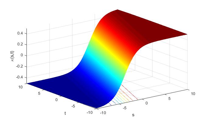
Figure 1: The kink soliton solution of $\kappa(s,t)$ for $A_{1}=0.5,A_{2}=1.$

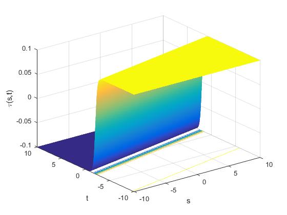
Figure 2: The kink soliton solution of $\tau(s,t)$ for $A_{1}=0.1,A_{2}=0.1.$

$$-A_{1}\eta\upsilon p_{1}\tanh^{p_{1}-1}\xi-A_{1}\eta\upsilon p_{1}\tanh^{p_{1}+1}\xi+A_{1}A_{2}\tanh^{p_{1}+p_{2}}\xi=0$$ (5.3)

and

$$A_{1}^{2}\eta^{2}p_{1}^{2}\tanh^{p_{1}+1}\xi(1+\tanh^{2}\xi)^{2}-A_{1}^{2}\eta^{2}p_{1}(p_{1}-1)\tanh^{2p_{1}-2}\xi(1+\tanh^{2}\xi)+A_{1}^{4}\tanh^{4p_{1}}\xi$$

$$-A_{1}^{2}\eta^{2}p_{1}(p_{1}+1)\tanh^{2p_{1}}\xi(1+\tanh^{2}\xi)+A_{1}^{2}A_{2}\eta\upsilon p_{2}\tanh^{2p_{1}+p_{2}-1}\xi(1+\tanh^{2}\xi)=0.$$ (5.4)

From (5.3) and (5.4), equating the coefficients of $(p_{1}+1,2p_{1})$ and $(2p_{1},2p_{1}+p_{2}-1)$ gives

$$p_{1}=p_{2}=1.$$ (5.5)

As a result, we obtain

$$\upsilon=\frac{\eta}{A_{2}},$$

where $\eta^{2}+A_{1}^{2}=1$. Hence, we get the kink soliton solution for (5.1) as

$$\kappa(s,t) = A_{1}\tanh(\eta(s-\upsilon t)),$$ (5.6)

$$\tau(s,t) = A_{2}\tanh(\eta(s-\upsilon t)).$$

Type 2 The evolution equations for the curvatures of the curve in terms of the velocities $\left\{\alpha,\beta,\gamma\right\}=\left\{\tau,\kappa_{s},\dfrac{\tau-\kappa_{ss}}{\kappa}\right\}$ obtained using (3.3) as

$$\kappa_{t} = \tau_{s}-\tau\kappa_{s},$$ (5.7)

$$\tau_{t} = \left(\frac{(2\tau\tau_{s}-\kappa_{sss})\kappa-(\tau^{2}-\kappa_{ss})\kappa_{s}}{\kappa^{2}}\right)+\kappa\kappa_{s}.$$

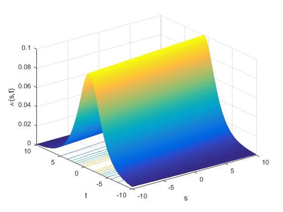
Figure 3: The bell-shaped soliton solution of $\kappa(s,t)$ for $B_{1}=0.1,B_{2}=-1.$

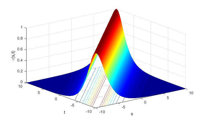
Figure 4: The bell-shaped soliton solution of $\tau(s,t)$ for $B_{1}=-1,B_{2}=1.$

We assume that the solutions are in the form

$$\kappa(s,t) = \frac{B_{1}}{\cosh^{1/p_{1}}\xi},$$ (5.8)

$$\tau(s,t) = \frac{B_{2}}{\cosh^{1/p_{2}}\xi},$$

with $\xi=\eta(s-\upsilon t)$, [19]. Substituting (5.8) into (5.7) yields

$$B_{1}\eta\upsilon\frac{1}{p_{1}}\frac{1}{\cosh^{1/p_{1}}\xi}+B_{2}\eta\frac{1}{p_{2}}\frac{1}{\cosh^{1/p_{2}}\xi}-B_{1}B_{2}\frac{1}{p_{1}}\frac{1}{\cosh^{1/p_{1}+1/p_{2}}\xi}=0.$$ (5.9)

and

$$B_{1}^{2}\eta\frac{1}{p_{1}}\frac{1}{\cosh^{2/p_{1}}\xi}+B_{2}\eta\upsilon\frac{1}{p_{2}}\frac{1}{\cosh^{1/p_{2}}\xi}+\frac{B_{2}^{2}}{B_{1}}\eta\left(-\frac{1}{p_{1}}+\frac{2}{p_{2}}\right)\frac{1}{\cosh^{1/p_{1}+2/p_{2}}\xi}.$$

$$+2\eta^{3}\left(-1-\frac{1}{p_{1}}\right)\frac{1}{p_{1}}\frac{1}{\cosh^{2}\xi}=0.$$ (5.10)

Now, from (5.10), equating the exponent $\left(\dfrac{2}{p_{1}},2\right)$ and $\left(\dfrac{-1}{p_{1}}+\dfrac{2}{p_{2}},\dfrac{1}{p_{2}}\right)$ leads to

$$p_{1}=p_{2}=1.$$ (5.11)

Consequently, we obtain

$$\upsilon=-\frac{B_{2}}{B_{1}},$$ (5.12)

where $\eta=\dfrac{B_{1}}{2}.$

We obtain following bell-shaped soliton solutions

$$\kappa(s,t) = \frac{B_{1}}{\cosh\xi}=B_{1}\sec h\xi,$$ (5.13)

$$\tau(s,t) = \frac{B_{2}}{\cosh\xi}=B_{2}\sec h\xi.$$

6 Conclusion

In this work, the evolutions of inextensible spacelike curves and timelike special ruled surfaces have been obtained. Then, we derived the evolution equations for the curvatures of the curve in terms of the velocities and found exact solutions. We have also found the kink solitary and bell-shaped wave solutions by ansatz method for the solutions of these equations. In Figs.1-2, the kink solitary waves of $\kappa(s,t)~{}$ and $\tau(s,t)~{}$ obtained by Eq. (5.6) are presented for values $A_{1}=0.5,A_{2}=1$ and $A_{1}=0.1,A_{2}=0.1$. The bell-shaped solitary waves of $\kappa(s,t)~{}$ and $\tau(s,t)~{}$ obtained by Eq. (5.13) are given by Figs. 3-4 for $B_{1}=0.1,B_{2}=-1$ and $B_{1}=-1,B_{2}=1$.

References

• [1] N. H. Abdel-All, R. A. Hussien, T. Youssef, (2012). Evolution of curves via the velocities of the moving frame. J Math. Comput. Sci., 2(5), 1170.
• [2] N. H. Abdel-All, M. A. Abdel-Razek, H. S. Abdel-Aziz, A. A Khalil, (2011). Geometry of evolving plane curves problem via lie group analysis. Stud. Math. Sci., 2(1), 51-62.
• [3] K. Alkan, S. C. Anco, (2016). Integrable systems from inelastic curve flows in 2–and 3–dimensional Minkowski space. J. Nonlinear Math. Phys., 23(2), 256-299.
• [4] R. Balakrishnan, R. Blumenfeld, (1997). Transformation of general curve evolution to a modified Belavin-Polyakov equation. J. Math. Phys., 38(11), 5878-5888.
• [5] M. Bektas, M. Kulahci, (2015). A Note on Inextensible Flows of Space-like Curves in Light-like Cone. Prespacetime J., 6(4), 313-321.
• [6] M. Carmo, Differential Geometry of Curves and Surfaces, Prentice-Hall, Saddle River, 1976.
• [7] J. H. Choi, H. Kim, (2017). Bell-shaped and kink-shaped solutions of the generalized Benjamin-Bona-Mahony-Burgers equation, Res. Phys., 7, 2369-2374.
• [8] O. Guner, (2017). Shock waves solution of nonlinear partial differential equation system by using the ansatz method. Optik, 130, 448-454.
• [9] N. Gurbuz, (2018). Three classes of non-lightlike curve evolution according to Darboux frame and geometric phase. Int. J. Geom. Methods Mod. Phys., 15, 1850023.
• [10] H. Hasimoto, (1959). A soliton on a vortex filament. J. Fluid Mech., 51(3), 477-485.
• [11] R. A. Hussien, T. Youssef, (2016). Evolution of special Ruled surfaces via the evolution of their directrices in Euclidean 3-space $E^{3}$. Appl. Math., 10(5), 1949-1956.
• [12] D.Y. Kwon, F. C. Park, (2005). Inextensible flows of curves and developable surfaces. Appl. Math. Lett., 18, 1156–1162.
• [13] M. Lakshmanan, T. W. Ruijgrok, C. J. Thompson, (1976). On the dynamics of a continuum spin system. Phys. A, 84(3), 577-590.
• [14] G. L. Lamb, (1977). Solitons on moving space curves. J. Math. Phys., 18, 1654-1661.
• [15] R. López, (2008). Differential geometry of curves and surfaces in Lorentz-Minkowski space. arXiv preprint arXiv:0810.3351.
• [16] B. O’Neill, Semi-Riemannian Geometry, Academic Press Inc., New York, 1983.
• [17] H. H. Uğurlu, H. Kocayigit, (1996). The Frenet and Darboux instantaneous rotain vectors of curves on time-like surfaces. Math. Compt. Appl., 1(2), 133-141.
• [18] F. Tchier, E. Cavlak Aslan, M. Inc, (2016). Optical solitons for cascaded system: Jacobi elliptic functions. J. Mod. Opt., 63(21), 2298-2307.
• [19] H. Triki, D. Milovic, A. Biswas, (2013). Solitary wave sand shock waves of the KdV6 equation. Ocean Eng., 73, 119-125.
• [20] V. D. l. Woestijne, (1988). Minimal surfaces of the 3-dimensional Minkowski space, Proc. Congres Geometrie differentielle et applications, Avignon , World Scientific Publishing, Singapore, 344-369.
• [21] O. G. Yildiz, M. Tosun, (2017). A Note on Evolution of Curves in the Minkowski Spaces. Adv. in Appl. Clifford Algebr., 27(3), 2873-2884.
• [22] Z. K. Yüzbaşı, D. W. Yoon, (2018). Inextensible Flows of Curves on Lightlike Surfaces. Mathematics, 6(11), 224.