Deep Non-Rigid Structure from Motion

Abstract

Current non-rigid structure from motion (NRSfM) algorithms are mainly limited with respect to: (i) the number of images, and (ii) the type of shape variability they can handle. This has hampered the practical utility of NRSfM for many applications within vision. In this paper we propose a novel deep neural network to recover camera poses and 3D points solely from an ensemble of 2D image coordinates. The proposed neural network is mathematically interpretable as a multi-layer block sparse dictionary learning problem, and can handle problems of unprecedented scale and shape complexity. Extensive experiments demonstrate the impressive performance of our approach where we exhibit superior precision and robustness against all available state-of-the-art works by an order of magnitude. We further propose a quality measure (based on the network weights) which circumvents the need for 3D ground-truth to ascertain the confidence we have in the reconstruction.

1 Introduction

Building an AI capable of inferring the 3D structure and pose of an object from a single image is a problem of immense importance. Training such a system using supervised learning requires a large number of labeled images – how to obtain these labels is currently an open problem for the vision community. Rendering [27] is problematic as the synthetic images seldom match the appearance and geometry of the objects we encounter in the real-world. Hand annotation is preferable, but current strategies rely on associating the natural images with an external 3D dataset (e.g. ShapeNet [8], ModelNet [32]), which we refer to as 3D supervision. If the 3D shape dataset does not capture the variation we see in the imagery, it is inherently ill-posed.

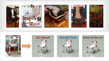
Figure 1: In this paper, we want to reconstruct 3D shapes solely from a sequence of annotated images—shown on top—with no need of 3D ground truth. Our proposed hierarchical sparse coding model and corresponding deep solution outperforms state-of-the-art by an order of magnitude.

Non-Rigid Structure from Motion (NRSfM) offers computer vision a way out of this quandary – by recovering the pose and 3D structure of an object category solely from hand annotated 2D landmarks with no need for 3D supervision. Classically [6], the problem of NRSfM has been applied to objects that move non-rigidly over time such as the human body and face. But NRSfM is not restricted to non-rigid objects; it can equally be applied to rigid objects whose object categories deform non-rigidly [19, 2, 30]. Consider, for example, the five objects in Figure 1 (top), instances from the visual object category “chair”. Each object in isolation represents a rigid chair, but the set of all 3D shapes describing “chair” is non-rigid. In other words, each object instance can be modeled as a deformation from its category’s general shape.

NRSfM is well-noted in literature as an ill-posed problem due to the non-rigidity. This has been mainly addressed by imposing additional shape priors, e.g. low rank [6, 10], union-of-subspaces [36, 2], and block-sparsity [18, 19]. However, low rank is only applicable to simple non-rigid objects with limited deformations and union-of-subspaces relies heavily on frame clustering which is still an open problem. Block-sparsity, where each shape can be represented by at most $K$ bases out of $L$, is considered as one of the most promising assumptions in terms of modeling broad shape variations. This is because sparsity can be thought of as a union of $\binom{L}{K}$ subspaces constraint and an over-complete dictionary could be utilized. However, it was noted by Kong et al. [18], that searching for the best subspace out of $\binom{L}{K}$ is extremely costly and not robust. Based on this observation we propose a novel shape prior that employs hierarchical sparse coding. The introduction of additional layers, in comparison to classical single-layer sparse coding, provides a mechanism for controlling the number of active subspaces. The ability of hierarchical sparse coding to provide a model that is both expressible and robust for general NRSfM forms the central thesis of our paper.

1.0.1 Contributions

• We propose a novel shape prior based on hierarchical sparse coding and demonstrate that the 2D projections under orthogonal cameras can be represented by the hierarchical dictionaries in a block sparse way.

• We designed a deep neural network to approximately solve the proposed hierarchical block sparse model and show how the network architecture is derived from a classical sparse coding algorithm.

• Finally, extensive experiments are conducted using various datasets. Both quantitative and qualitative results demonstrate our superior performance, outperforming all state-of-the-arts in the order of magnitude.

2 Related Work

2.0.1 Low-rank NRSfM

In rigid structure from motion, the rank of 3D structure is fixed as three [29] since 3D shapes remain the same between frames. Based on this insight, Bregler et al. [6] advocated that non-rigid 3D structure could be represented by a linear subspace of low rank. Dai et al. [10] developed this prior by proving that low-rank assumption itself is sufficient to address the ill-posedness of NRSfM with no need of additional priors. The low-rank assumption has also been applied temporally [3, 15] – 3D point trajectories can be represented by pre-defined (e.g. DCT) or learned bases. Although exhibiting impressive performance, the low-rank assumption has a major drawback. The rank is strictly limited by the number of points and frames (whichever is smaller [10]). This makes low-rank NRSfM infeasible if we want to solve large-scale problems with complex shape variations when the number of points is substantially smaller than the number of frames.

2.0.2 Union-of-subspaces NRSfM

Inspired by an intuition that complex non-rigid deformations could be clustered into a sequence of simple motions, Zhu et al. [36] proposed to model non-rigid 3D structure by a union of local subspaces. This was later extended to spatial-temporal domain [1] and applied to rigid object category reconstruction [2]. The major difficulty of union-of-subspaces is how to effectively cluster shape deformations purely from 2D observations and how to estimate affinity matrix when the number of frame is large e.g. more than tens of thousand frames.

2.0.3 Sparse NRSfM

Sparse prior [18, 35, 19] is more generic than union-of-subspaces since it is equivalent to the union of all possible local subspaces. One obvious advantages of this is the large number of subspaces enables the effective modeling of a broader set of 3D structures. However, the sheer number of subspaces that can be entertained by the sparsity prior is its fundamental drawback. Since there are so many possible subspaces to choose from, the approach is sensitive to noise, dramatically limiting its applicability to “real-world” NRSfM problems. In this paper we want to leverage the elegance and expressibility of the sparsity prior without suffering from its inherent sensitivity to noise.

3 Background

Sparse dictionary learning can be considered as an unsupervised learning task and divided into two sub-problems: (i) dictionary learning, and (ii) sparse code recovery. Let us consider sparse code recovery problem, where we estimate a sparse representation $\mathbf{z}$ for a measurement vector $\mathbf{x}$ given the dictionary $\mathbf{D}$ i.e.

$$\min_{\mathbf{z}}\|\mathbf{x}-\mathbf{D}\mathbf{z}\|_{2}^{2}\quad\ \mathrm{s.t.}\ \|\mathbf{z}\|_{0}<\lambda,$$ (1)

where $\lambda$ related to the trust region controls the sparsity of recovered code. One classical algorithm to recover the sparse representation is Iterative Shrinkage and Thresholding Algorithm (ISTA) [11, 26, 5]. ISTA iteratively executes the following two steps with $\mathbf{z}^{[0]}=\mathbf{0}$:

$$\mathbf{v}=\mathbf{z}^{[i]}-\alpha\mathbf{D}^{T}(\mathbf{D}\mathbf{z}^{[i]}-\mathbf{x}),$$ (2)

$$\mathbf{z}^{[i+1]}=\operatorname*{argmin}_{\mathbf{u}}\frac{1}{2}\|\mathbf{u}-\mathbf{v}\|^{2}_{2}+\tau\|\mathbf{u}\|_{1},$$ (3)

which first uses the gradient of $\|\mathbf{x}-\mathbf{D}\mathbf{z}\|_{2}^{2}$ to update $\mathbf{z}^{[i]}$ in step size $\alpha$ and then finds the closest sparse solution using an $\ell_{1}$ convex relaxation. It is well known in literature that the second step has a closed-form solution using the soft thresholding operator. Therefore, ISTA can be summarized as the following recursive equation:

$$\mathbf{z}^{[i+1]}=h_{\tau}\big{(}\mathbf{z}^{[i]}-\alpha\mathbf{D}^{T}(\mathbf{D}\mathbf{z}^{[i]}-\mathbf{x})\big{)},$$ (4)

where $h_{\tau}$ is a soft thresholding operator and $\tau$ is related to $\lambda$ for controlling sparsity.

Recently, Papyan [25] proposed to use ISTA and sparse coding to reinterpret feed-forward neural networks. They argue that feed-forward passing a single-layer neural network $\mathbf{z}=\mathop{\mathrm{ReLU}}(\mathbf{D}^{T}\mathbf{x}-b)$ can be considered as one iteration of ISTA when $\mathbf{z}~{}\geq~{}0,\alpha=1$ and $\tau=b$. Based on this insight, the authors extend this interpretation to feed-forward neural network with $n$ layers

$$\mathbf{z}_{1} =\mathop{\mathrm{ReLU}}(\mathbf{D}_{1}^{T}\mathbf{x}-b_{1})$$ (5)

$$\mathbf{z}_{2} =\mathop{\mathrm{ReLU}}(\mathbf{D}_{2}^{T}\mathbf{z}_{1}-b_{2})$$

$$\quad\vdots$$

$$\mathbf{z}_{n} =\mathop{\mathrm{ReLU}}(\mathbf{D}_{n}^{T}\mathbf{z}_{n-1}-b_{n})$$

as executing a sequence of single-iteration ISTA, serving as an approximate solution to the multi-layer sparse coding problem: find $\{\mathbf{z}_{i}\}_{i=1}^{n}$, such that

$$\mathbf{x}=\mathbf{D}_{1}\mathbf{z}_{1} ,\quad\|\mathbf{z}_{1}\|_{0}<\lambda_{1},\mathbf{z}_{1}\geq 0,$$ (6)

$$\mathbf{z}_{1}=\mathbf{D}_{2}\mathbf{z}_{2} ,\quad\|\mathbf{z}_{2}\|_{0}<\lambda_{2},\mathbf{z}_{2}\geq 0,$$

$$\vdots ,\quad\quad\vdots$$

$$\mathbf{z}_{n-1}=\mathbf{D}_{n}\mathbf{z}_{n} ,\quad\|\mathbf{z}_{n}\|_{0}<\lambda_{n},\mathbf{z}_{n}\geq 0,$$

where the bias terms $\{b_{i}\}_{i=1}^{n}$ (in a similar manner to $\tau$) are related to $\{\lambda_{i}\}_{i=1}^{n}$, adjusting the sparsity of recovered code. Furthermore, they reinterpret back-propagating through the deep neural network as learning the dictionaries $\{\mathbf{D}_{i}\}_{i=1}^{n}$. This connection offers a novel breakthrough for understanding DNNs. In this paper, we extend this to the block sparse scenario and apply it to solving our NRSfM problem.

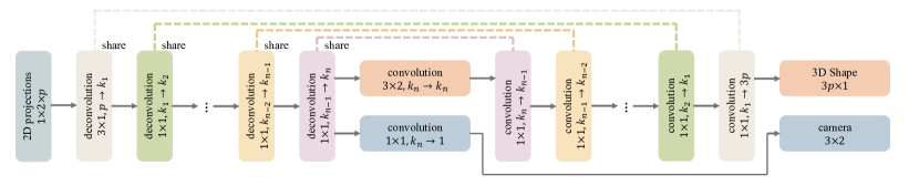
Figure 2: Deep NRSfM architecture. The network can be divided into two parts: encoder and decoder that are symmetric and share convolution kernels (i.e. dictionaries). The symbol $a\times b,c\to d$ refers to the operator using kernel size $a\times b$ with $c$ input channels and $d$ output channels.

4 Deep Non-Rigid Structure from Motion

Under orthogonal projection, NRSfM deals with the problem of factorizing a 2D projection matrix $\mathbf{W}\in\mathbb{R}^{p\times 2}$ as the product of a 3D shape matrix $\mathbf{S}\in\mathbb{R}^{p\times 3}$ and camera matrix $\mathbf{M}\in\mathbb{R}^{3\times 2}$. Formally,

$$\mathbf{W}=\mathbf{S}\mathbf{M},$$ (7)

$$\mathbf{W}=\begin{bmatrix}u_{1}&v_{1}\\ u_{2}&v_{2}\\ \vdots&\vdots\\ u_{p}&v_{p}\end{bmatrix},~{}\mathbf{S}=\begin{bmatrix}x_{1}&y_{1}&z_{1}\\ x_{2}&y_{2}&z_{2}\\ \vdots&\vdots&\vdots\\ x_{p}&y_{p}&z_{p}\end{bmatrix},~{}\mathbf{M}^{T}\mathbf{M}=\mathbf{I}_{2},$$ (8)

where $(u_{i},v_{i}),(x_{i},y_{i},z_{i})$ are the image and world coordinates of the $i$-th point. The goal of NRSfM is to recover simultaneously the shape $\mathbf{S}$ and the camera $\mathbf{M}$ for each projection $\mathbf{W}$ in a given set $\mathbb{W}$ of 2D landmarks. In a general NRSfM including SfC, this set $\mathbb{W}$ could contain deformations of a non-rigid object or various instances from an object category.

4.1 Modeling via multi-layer sparse coding

To alleviate the ill-posedness of NRSfM and also guarantee sufficient freedom on shape variation, we propose a novel prior assumption on 3D shapes via multi-layer sparse coding: The vectorization of $\mathbf{S}$ satisfies

$$\mathbf{s}=\mathbf{D}_{1}\boldsymbol{\psi}_{1} ,\quad\|\boldsymbol{\psi}_{1}\|_{0}<\lambda_{1},\boldsymbol{\psi}_{1}\geq 0,$$ (9)

$$\boldsymbol{\psi}_{1}=\mathbf{D}_{2}\boldsymbol{\psi}_{2} ,\quad\|\boldsymbol{\psi}_{2}\|_{0}<\lambda_{2},\boldsymbol{\psi}_{2}\geq 0,$$

$$\vdots ,\quad\quad\vdots$$

$$\boldsymbol{\psi}_{n-1}=\mathbf{D}_{n}\boldsymbol{\psi}_{n} ,\quad\|\boldsymbol{\psi}_{n}\|_{0}<\lambda_{n},\boldsymbol{\psi}_{n}\geq 0,$$

where $\mathbf{D}_{1}\in\mathbb{R}^{3p\times k_{1}},\mathbf{D}_{2}\in\mathbb{R}^{k_{1}\times k_{2}},\dots,\mathbf{D}_{n}\in\mathbb{R}^{k_{n-1}\times k_{n}}$ are hierarchical dictionaries. In this prior, each non-rigid shape is represented by a sequence of hierarchical dictionaries and corresponding sparse codes. Each sparse code is determined by its lower-level neighbor and affects the next-level. Clearly this hierarchy adds more parameters, and thus more freedom into the system. We now show that it paradoxically results in a more constrained global dictionary and sparse code recovery.

4.1.1 More constrained code recovery

In a classical single dictionary system, the constraint on the representation is element-wise sparsity. Further, the quality of its recovery entirely depends on the quality of the dictionary. In our multi-layer sparse coding model, the optimal code not only minimizes the difference between measurements $\mathbf{s}$ and $\mathbf{D}_{1}\boldsymbol{\psi}_{1}$ along with sparsity regularization $\|\boldsymbol{\psi}_{1}\|_{0}$, but also satisfies constraints from its subsequent representations. This additional joint inference imposes more constraints on code recovery, helps to control the uniqueness and therefore alleviates its heavy dependency on the dictionary quality.

4.1.2 More constrained dictionary

When all equality constraints are satisfied, the multi-layer sparse coding model degenerates to a single dictionary system. From Equation 9, by denoting $\mathbf{D}^{(l)}=\prod_{i=1}^{l}\mathbf{D}_{i}$, it is implied that $\mathbf{s}=\mathbf{D}_{1}\mathbf{D}_{2}\dots\mathbf{D}_{n}\boldsymbol{\psi}_{n}=\mathbf{D}^{(n)}\boldsymbol{\psi}_{n}$. However, this differs from other single dictionary models [36, 37, 18, 19, 34] in terms that a unique structure is imposed on $\mathbf{D}^{(n)}$ [28]. The dictionary $\mathbf{D}^{(n)}$ is composed by simpler atoms hierarchically. For example, each column of $\mathbf{D}^{(2)}=\mathbf{D}_{1}\mathbf{D}_{2}$ is a linear combination of atoms in $\mathbf{D}_{1}$, each column of $\mathbf{D}^{(3)}=\mathbf{D}^{(2)}\mathbf{D}_{3}$ is a linear combination of atoms in $\mathbf{D}^{(2)}$ and so on. Such a structure results in a more constrained global dictionary and potentially leads to higher quality with lower mutual coherence [14].

4.2 Multi-layer block sparse coding

Given the proposed multi-layer sparse coding model, we now build a conduit from the proposed shape code $\{\boldsymbol{\psi}_{i}\}_{i=1}^{k}$ to the 2D projected points. From Equation 9, we reshape vector $\mathbf{s}$ to a matrix $\mathbf{S}\in\mathbb{R}^{p\times 3}$ such that $\mathbf{S}=\mathbf{D}^{\sharp}_{1}(\boldsymbol{\psi}_{1}\otimes\mathbf{I}_{3})$, where $\otimes$ is Kronecker product and $\mathbf{D}_{1}^{\sharp}\in\mathbb{R}^{p\times 3k_{1}}$ is a reshape of $\mathbf{D}_{1}$ [10]. From linear algebra, it is well known that $\mathbf{A}\mathbf{B}\otimes\mathbf{I}=(\mathbf{A}\otimes\mathbf{I})(\mathbf{B}\otimes\mathbf{I})$ given three matrices $\mathbf{A},\mathbf{B}$, and identity matrix $\mathbf{I}$. Based on this lemma, we can derive that

$$\mathbf{S}=\mathbf{D}^{\sharp}_{1}(\boldsymbol{\psi}_{1}\otimes\mathbf{I}_{3}) ,\quad\|\boldsymbol{\psi}_{1}\|_{0}<\lambda_{1},\boldsymbol{\psi}_{1}\geq 0,$$ (10)

$$\boldsymbol{\psi}_{1}\otimes\mathbf{I}_{3}=(\mathbf{D}_{2}\otimes\mathbf{I}_{3})(\boldsymbol{\psi}_{2}\otimes\mathbf{I}_{3}) ,\quad\|\boldsymbol{\psi}_{2}\|_{0}<\lambda_{2},\boldsymbol{\psi}_{2}\geq 0,$$

$$\vdots ,\quad\quad\vdots$$

$$\boldsymbol{\psi}_{n-1}\otimes\mathbf{I}_{3}=(\mathbf{D}_{n}\otimes\mathbf{I}_{3})(\boldsymbol{\psi}_{n}\otimes\mathbf{I}_{3}) ,\quad\|\boldsymbol{\psi}_{n}\|_{0}<\lambda_{n},\boldsymbol{\psi}_{n}\geq 0.$$

Further, from Equation 7, by right multiplying the camera matrix $\mathbf{M}\in\mathbb{R}^{3\times 2}$ to the both sides of Equation 10 and denote $\boldsymbol{\Psi}_{i}=\boldsymbol{\psi}_{i}\otimes\mathbf{M}$, we obtain that

$$\mathbf{W}=\mathbf{D}^{\sharp}_{1}\boldsymbol{\Psi}_{1} ,\quad\|\boldsymbol{\Psi}_{1}\|_{0}^{(3\times 2)}<\lambda_{1},$$ (11)

$$\boldsymbol{\Psi}_{1}=(\mathbf{D}_{2}\otimes\mathbf{I}_{3})\boldsymbol{\Psi}_{2} ,\quad\|\boldsymbol{\Psi}_{2}\|_{0}^{(3\times 2)}<\lambda_{2},$$

$$\vdots ,\quad\quad\vdots$$

$$\boldsymbol{\Psi}_{n-1}=(\mathbf{D}_{n}\otimes\mathbf{I}_{3})\boldsymbol{\Psi}_{n} ,\quad\|\boldsymbol{\Psi}_{n}\|_{0}^{(3\times 2)}<\lambda_{n},$$

where $\|\cdot\|_{0}^{(3\times 2)}$ divides the argument matrix into blocks with size $3\times 2$ and counts the number of active blocks. Since $\boldsymbol{\psi}_{i}$ has active elements less than $\lambda_{i}$, $\boldsymbol{\Psi}_{i}$ has active blocks less than $\lambda_{i}$, that is $\boldsymbol{\Psi}_{i}$ is block sparse. This derivation demonstrates that if the shape vector $\mathbf{s}$ satisfies the multi-layer sparse coding prior described by Equation 9, then its 2D projection $\mathbf{W}$ must be in the format of multi-layer block sparse coding described by Equation 11. We hereby interpret NRSfM as a hierarchical block sparse dictionary learning problem i.e. factorizing $\mathbf{W}$ as products of hierarchical dictionaries $\{\mathbf{D}_{i}\}_{i=1}^{n}$ and block sparse coefficients $\{\boldsymbol{\Psi}_{i}\}_{i=1}^{n}$.

4.3 Block ISTA and DNNs solution

Before solving the multi-layer block sparse coding problem in Equation 11, we first consider the single-layer problem:

$$\min_{\mathbf{Z}}\|\mathbf{X}-\mathbf{D}\mathbf{Z}\|_{F}^{2}\quad\ \mathrm{s.t.}\ ~{}\|\mathbf{Z}\|_{0}^{(3\times 2)}<\lambda.$$ (12)

Inspired by ISTA, we propose to solve this problem by iteratively executing the following two steps:

$$\mathbf{V}=\mathbf{Z}^{[i]}-\alpha\mathbf{D}^{T}(\mathbf{D}\mathbf{Z}^{[i]}-\mathbf{X}),$$ (13)

$$\mathbf{Z}^{[i+1]}=\operatorname*{argmin}_{\mathbf{U}}\frac{1}{2}\|\mathbf{U}-\mathbf{V}\|^{2}_{F}+\tau\|\mathbf{U}\|_{F1}^{(3\times 2)},$$ (14)

where $\|\cdot\|_{F1}^{(3\times 2)}$ is defined as the summation of Frobenius norm of each $3\times 2$ block, serving as a convex relaxation of block sparsity constraint. It is derived in [13] that the second step has a closed-form solution computing each block separately by $\small\mathbf{Z}^{[i+1]}_{j}=(h_{\tau}(\|\mathbf{V}_{j}\|_{F})/\|\mathbf{V}_{j}\|_{F})\mathbf{V}_{j}$, where the subscript $j$ represents the $j$-th block and $h_{\tau}$ is a soft thresholding operator. However, soft thresholding the Frobenius norms for every block brings unnecessary computational complexity. We show in the supplementary material that an efficient approximation is $\mathbf{Z}^{[i+1]}_{j}=h_{b_{j}}(\mathbf{V}_{j})$, where $b_{j}$ is the threshold for the $j$-th block, controlling its sparsity. Based on this approximation, a single-iteration block ISTA with step size $\alpha=1$ can be represented by :

$$\mathbf{Z}=h_{\mathbf{b}}\big{(}\mathbf{D}^{T}\mathbf{X}\big{)}=\mathop{\mathrm{ReLU}}(\mathbf{D}^{T}\mathbf{X}-\mathbf{b}\otimes\mathbf{1}_{3\times 2}),$$ (15)

where $h_{\mathbf{b}}$ is a soft thresholding operator using the $j$-th element $b_{j}$ as threshold of the $j$-th block and the second equality holds if $\mathbf{Z}$ is non-negative.

4.3.1 Encoder

Recall from Section 3 that the feed-forward pass through a deep neural network can be considered as a sequence of single ISTA iterations and thus provides an approximate recovery of multi-layer sparse codes. We follow the same scheme: we first assume the multi-layer block sparse coding to be non-negative and then sequentially use single-iteration block ISTA to solve it i.e.

$$\boldsymbol{\Psi}_{1} =\mathop{\mathrm{ReLU}}((\mathbf{D}^{\sharp}_{1})^{T}\mathbf{W}-\mathbf{b}_{1}\otimes\mathbf{1}_{3\times 2}),$$ (16)

$$\boldsymbol{\Psi}_{2} =\mathop{\mathrm{ReLU}}((\mathbf{D}_{2}\otimes\mathbf{I}_{3})^{T}\boldsymbol{\Psi}_{1}-\mathbf{b}_{2}\otimes\mathbf{1}_{3\times 2}),$$

$$\quad\vdots$$

$$\boldsymbol{\Psi}_{n} =\mathop{\mathrm{ReLU}}((\mathbf{D}_{n}\otimes\mathbf{I}_{3})^{T}\boldsymbol{\Psi}_{n-1}-\mathbf{b}_{n}\otimes\mathbf{1}_{3\times 2}),$$

where thresholds $\mathbf{b}_{1},...,\mathbf{b}_{n}$ are learned, controlling the block sparsity. This learning is crucial because in previous NRSfM algorithms utilizing low-rank [10], subspaces [36] or compressible [18] priors, the weight given to this prior (e.g. rank or sparsity) is hand-selected through a cumbersome cross validation process. In our approach, this weighting is learned simultaneously with all other parameters removing the need for any irksome cross validation process. This formula composes the encoder of our proposed DNN.

4.3.2 Decoder

Let us for now assume that we can extract camera $\mathbf{M}$ and regular sparse hidden code $\boldsymbol{\psi}_{n}$ from $\boldsymbol{\Psi}_{n}$ by some functions i.e. $\mathbf{M}=\mathcal{F}(\boldsymbol{\Psi}_{n})$ and $\boldsymbol{\psi}_{n}=\mathcal{G}(\boldsymbol{\Psi}_{n})$, which will be discussed in the next section. Then we can compute the 3D shape vector $\mathbf{s}$ by:

$$\boldsymbol{\psi}_{n-1} =\mathop{\mathrm{ReLU}}(\mathbf{D}_{n}\boldsymbol{\psi}_{n}-\mathbf{b}_{n}^{\prime}),$$ (17)

$$\quad\vdots$$

$$\boldsymbol{\psi}_{1} =\mathop{\mathrm{ReLU}}(\mathbf{D}_{2}\boldsymbol{\psi}_{2}-\mathbf{b}_{2}^{\prime}),$$

$$\mathbf{s} =\mathbf{D}^{\sharp}_{1}\boldsymbol{\psi}_{1},$$

Note we preserve the ReLU and bias term during decoding to further enforce sparsity and improve robustness. These portion forms the decoder of our DNN.

4.3.3 Variation of implementation

The Kronecker product of identity matrix $\mathbf{I}_{3}$ dramatically increases the time and space complexity of our approach. To eliminate it and make parameter sharing easier in modern deep learning environments (e.g. TensorFlow, PyTorch), we reshape the filters and features and show that the matrix multiplication in each step of the encoder and decoder can be equivalently computed via multi-channel $1\times 1$ convolution ($*$) and transposed convolution ($*^{T}$) i.e.

$$(\mathbf{D}_{1}^{\sharp})^{T}\mathbf{W}=\mathsf{d}_{1}^{\sharp}*^{T}\mathsf{w},$$ (18)

where $\mathsf{d}_{1}^{\sharp}\in\mathbb{R}^{3\times 1\times k_{1}\times p},\mathsf{w}\in\mathbb{R}^{1\times 2\times p}$.

$$(\mathbf{D}_{i+1}\otimes\mathbf{I}_{3})^{T}\boldsymbol{\Psi}_{i}=\mathsf{d}_{i+1}*^{T}\Psi_{i},$$ (19)

where $\mathsf{d}_{i+1}\in\mathbb{R}^{1\times 1\times k_{i+1}\times k_{i}},\Psi_{i}\in\mathbb{R}^{3\times 2\times k_{i}}.$

$$\mathbf{D}_{i}\boldsymbol{\psi}_{i}=\mathsf{d}_{i}*\psi_{i},$$ (20)

where $\mathsf{d}_{i}\in\mathbb{R}^{1\times 1\times k_{i}\times k_{i-1}},\psi_{i}\in\mathbb{R}^{1\times 1\times k_{i}}.$

4.3.4 Code and camera recovery

Estimating $\boldsymbol{\psi}_{n}$ and $\mathbf{M}$ from $\boldsymbol{\Psi}_{n}$ is discussed in [18] and solved by a closed-form formula. Due to its differentiability, we could insert the solution directly within our pipeline. An alternative solution is using an approximation i.e. a fully connected layer connecting $\boldsymbol{\Psi}_{n}$ and $\boldsymbol{\psi}_{n}$ and a linear combination among each blocks of $\boldsymbol{\Psi}_{n}$ to estimate $\mathbf{M}$, where the fully connected layer parameters and combination coefficients are learned from data. In our experiments, we use the approximate solution and represent them via convolutions, as shown in Figure 2, for conciseness and maintaining proper dimensions. Since the approximation has no way to force the orthonormal constraint on the camera, we seek help from the loss function.

4.3.5 Loss function

The loss function must measure the reprojection error between input 2D points $\mathbf{W}$ and reprojected 2D points $\mathbf{S}\mathbf{M}$ while simultaneously encouraging orthonormality of the estimated camera $\mathbf{M}$. One solution is to use spectral norm regularization of $\mathbf{M}$ because spectral norm minimization is the tightest convex relaxation of the orthonormal constraint [34]. An alternative solution is to hard code the singular values of $\mathbf{M}$ to be exact ones with the help of Singular Value Decomposition (SVD). Even though SVD is generally non-differentiable, the numeric computation of SVD is differentiable and most deep learning packages implement its gradients (e.g. PyTorch, TensorFlow). In our implementation and experiments, we use SVD to ensure the success of the orthonormal constraint and a simple Frobenius norm to measure reprojection error,

$$Loss=\|\mathbf{W}-\mathbf{S}\tilde{\mathbf{M}}\|_{F},\quad\tilde{\mathbf{M}}=\mathbf{U}\mathbf{V}^{T},$$ (21)

where $\mathbf{U}\boldsymbol{\Sigma}\mathbf{V}^{T}=\mathbf{M}$ is the SVD of the camera matrix.

[HTML]EFEFEFFurnitures	[HTML]EFEFEFBed	[HTML]EFEFEFChair	[HTML]EFEFEFSofa	[HTML]EFEFEFTable	[HTML]EFEFEFMean	[HTML]EFEFEFRelative
[HTML]EFEFEFKSTA [16]	0.069	0.158	0.066	0.217	[HTML]EFEFEF0.128	[HTML]EFEFEF12.19
[HTML]EFEFEFBMM [10]	0.059	0.330	0.245	0.211	[HTML]EFEFEF0.211	[HTML]EFEFEF20.12
[HTML]EFEFEFCNR [20]	0.227	0.163	0.835	0.186	[HTML]EFEFEF0.352	[HTML]EFEFEF33.55
[HTML]EFEFEFNLO [12]	0.245	0.339	0.158	0.275	[HTML]EFEFEF0.243	[HTML]EFEFEF23.18
[HTML]EFEFEFRIKS [17]	0.202	0.135	0.048	0.218	[HTML]EFEFEF0.117	[HTML]EFEFEF11.13
[HTML]EFEFEFSPS [18]	0.971	0.946	0.955	0.280	[HTML]EFEFEF0.788	[HTML]EFEFEF74.96
[HTML]EFEFEFSFC [19]	0.247	0.195	0.233	0.193	[HTML]EFEFEF0.217	[HTML]EFEFEF20.67
[HTML]EFEFEFOURS	0.004	0.019	0.005	0.012	[HTML]EFEFEF0.010	[HTML]EFEFEF1.00

Table 1: Quantitative comparison against state-of-the-art algorithms using IKEA dataset in normalized 3D error.

[HTML]EFEFEFMethods	[HTML]EFEFEFKSTA [16]		[HTML]EFEFEFBMM [10]		[HTML]EFEFEFCNS [20]		[HTML]EFEFEFMUS [2]		[HTML]EFEFEFNLO [12]		[HTML]EFEFEFRIKS [17]		[HTML]EFEFEFSPS [18]		[HTML]EFEFEFSFC [19]		[HTML]EFEFEFOURS
[HTML]EFEFEFAeroplane	0.145	[HTML]EFEFEF0.175	0.843	[HTML]EFEFEF1.459	0.263	[HTML]EFEFEF0.416	0.261	[HTML]EFEFEF-	-	[HTML]EFEFEF0.876	-	[HTML]EFEFEF0.132	-	[HTML]EFEFEF0.930	-	[HTML]EFEFEF0.504	-	[HTML]EFEFEF0.024
[HTML]EFEFEFBicycle	0.442	[HTML]EFEFEF0.245	0.308	[HTML]EFEFEF1.376	-	[HTML]EFEFEF0.356	0.178	[HTML]EFEFEF-	-	[HTML]EFEFEF0.269	-	[HTML]EFEFEF0.136	-	[HTML]EFEFEF1.322	-	[HTML]EFEFEF0.372	-	[HTML]EFEFEF0.003
[HTML]EFEFEFBus	0.214	[HTML]EFEFEF0.199	0.300	[HTML]EFEFEF1.023	-	[HTML]EFEFEF0.250	0.113	[HTML]EFEFEF-	-	[HTML]EFEFEF0.140	-	[HTML]EFEFEF0.160	-	[HTML]EFEFEF0.604	-	[HTML]EFEFEF0.251	-	[HTML]EFEFEF0.004
[HTML]EFEFEFCar	0.159	[HTML]EFEFEF0.152	0.266	[HTML]EFEFEF1.278	0.099	[HTML]EFEFEF0.258	0.078	[HTML]EFEFEF-	-	[HTML]EFEFEF0.104	-	[HTML]EFEFEF0.097	-	[HTML]EFEFEF0.872	-	[HTML]EFEFEF0.282	-	[HTML]EFEFEF0.009
[HTML]EFEFEFChair	0.399	[HTML]EFEFEF0.186	0.357	[HTML]EFEFEF1.297	-	[HTML]EFEFEF0.170	0.210	[HTML]EFEFEF-	-	[HTML]EFEFEF0.146	-	[HTML]EFEFEF0.192	-	[HTML]EFEFEF1.046	-	[HTML]EFEFEF0.226	-	[HTML]EFEFEF0.007
[HTML]EFEFEFDiningtable	0.372	[HTML]EFEFEF0.267	0.422	[HTML]EFEFEF1.00	-	[HTML]EFEFEF0.170	0.264	[HTML]EFEFEF-	-	[HTML]EFEFEF0.109	-	[HTML]EFEFEF0.207	-	[HTML]EFEFEF1.050	-	[HTML]EFEFEF0.221	-	[HTML]EFEFEF0.060
[HTML]EFEFEFMotorbike	0.270	[HTML]EFEFEF0.255	0.336	[HTML]EFEFEF0.857	-	[HTML]EFEFEF0.457	0.222	[HTML]EFEFEF-	-	[HTML]EFEFEF0.432	-	[HTML]EFEFEF0.118	-	[HTML]EFEFEF0.986	-	[HTML]EFEFEF0.361	-	[HTML]EFEFEF0.002
[HTML]EFEFEFSofa	0.298	[HTML]EFEFEF0.307	0.279	[HTML]EFEFEF1.126	0.214	[HTML]EFEFEF0.250	0.167	[HTML]EFEFEF-	-	[HTML]EFEFEF0.149	-	[HTML]EFEFEF0.228	-	[HTML]EFEFEF1.328	-	[HTML]EFEFEF0.302	-	[HTML]EFEFEF0.004
[HTML]EFEFEFAverage	0.287	[HTML]EFEFEF0.223	0.388	[HTML]EFEFEF1.178	0.192	[HTML]EFEFEF0.291	0.186	[HTML]EFEFEF-	-	[HTML]EFEFEF0.278	-	[HTML]EFEFEF0.159	-	[HTML]EFEFEF1.017	-	[HTML]EFEFEF0.315	-	[HTML]EFEFEF0.014
[HTML]EFEFEFRelative	-	[HTML]EFEFEF15.33	-	[HTML]EFEFEF80.76	-	[HTML]EFEFEF19.95	-	[HTML]EFEFEF-	-	[HTML]EFEFEF19.09	-	[HTML]EFEFEF10.92	-	[HTML]EFEFEF69.74	-	[HTML]EFEFEF21.61	-	[HTML]EFEFEF1.00
[HTML]EFEFEFAeroplane	0.183	[HTML]EFEFEF0.207	0.566	[HTML]EFEFEF1.465	0.294	[HTML]EFEFEF0.460	0.271	[HTML]EFEFEF-	-	[HTML]EFEFEF0.758	-	[HTML]EFEFEF0.146	-	[HTML]EFEFEF0.888	-	[HTML]EFEFEF0.521	-	[HTML]EFEFEF0.032
[HTML]EFEFEFBicycle	0.457	[HTML]EFEFEF0.232	0.307	[HTML]EFEFEF1.404	-	[HTML]EFEFEF0.359	0.188	[HTML]EFEFEF-	-	[HTML]EFEFEF0.275	-	[HTML]EFEFEF0.139	-	[HTML]EFEFEF0.851	-	[HTML]EFEFEF0.379	-	[HTML]EFEFEF0.007
[HTML]EFEFEFBus	0.218	[HTML]EFEFEF0.197	0.255	[HTML]EFEFEF0.764	-	[HTML]EFEFEF0.264	0.122	[HTML]EFEFEF-	-	[HTML]EFEFEF0.141	-	[HTML]EFEFEF0.159	-	[HTML]EFEFEF1.110	-	[HTML]EFEFEF0.264	-	[HTML]EFEFEF0.021
[HTML]EFEFEFCar	0.164	[HTML]EFEFEF0.139	0.161	[HTML]EFEFEF1.744	0.122	[HTML]EFEFEF0.265	0.093	[HTML]EFEFEF-	-	[HTML]EFEFEF0.105	-	[HTML]EFEFEF0.102	-	[HTML]EFEFEF0.804	-	[HTML]EFEFEF0.281	-	[HTML]EFEFEF0.010
[HTML]EFEFEFChair	0.396	[HTML]EFEFEF0.203	0.258	[HTML]EFEFEF1.197	-	[HTML]EFEFEF0.171	0.220	[HTML]EFEFEF-	-	[HTML]EFEFEF0.145	-	[HTML]EFEFEF0.193	-	[HTML]EFEFEF1.016	-	[HTML]EFEFEF0.223	-	[HTML]EFEFEF0.017
[HTML]EFEFEFDiningtable	0.383	[HTML]EFEFEF0.249	0.358	[HTML]EFEFEF1.105	-	[HTML]EFEFEF0.172	0.267	[HTML]EFEFEF-	-	[HTML]EFEFEF0.114	-	[HTML]EFEFEF0.227	-	[HTML]EFEFEF1.213	-	[HTML]EFEFEF0.222	-	[HTML]EFEFEF0.034
[HTML]EFEFEFMotorbike	0.290	[HTML]EFEFEF0.227	0.299	[HTML]EFEFEF1.117	-	[HTML]EFEFEF0.459	0.233	[HTML]EFEFEF-	-	[HTML]EFEFEF0.254	-	[HTML]EFEFEF0.125	-	[HTML]EFEFEF0.915	-	[HTML]EFEFEF0.351	-	[HTML]EFEFEF0.011
[HTML]EFEFEFSofa	0.294	[HTML]EFEFEF0.436	0.240	[HTML]EFEFEF1.143	0.228	[HTML]EFEFEF0.255	0.174	[HTML]EFEFEF-	-	[HTML]EFEFEF0.152	-	[HTML]EFEFEF0.239	-	[HTML]EFEFEF1.164	-	[HTML]EFEFEF0.306	-	[HTML]EFEFEF0.008
[HTML]EFEFEFAverage	0.298	[HTML]EFEFEF0.236	0.305	[HTML]EFEFEF1.232	0.215	[HTML]EFEFEF0.300	0.196	[HTML]EFEFEF-	-	[HTML]EFEFEF0.243	-	[HTML]EFEFEF0.166	-	[HTML]EFEFEF0.995	-	[HTML]EFEFEF0.318	-	[HTML]EFEFEF0.017
[HTML]EFEFEFRelative	-	[HTML]EFEFEF16.90	-	[HTML]EFEFEF88.78	-	[HTML]EFEFEF21.49	-	[HTML]EFEFEF-	-	[HTML]EFEFEF17.39	-	[HTML]EFEFEF11.90	-	[HTML]EFEFEF71.11	-	[HTML]EFEFEF22.78	-	[HTML]EFEFEF1.27

Table 2: Quantitative evaluation on PASCAL3D+ dataset. We conduct experiments on both original and noisy 2D annotations, listed at the upper and lower half of table respectively. The symbol ‘-’ indicates either algorithm implementation or data is missing. The shaded columns are erros using our processed data and others are copied from Table 2 in [2]. Relative errors are computed with respect to our method, the most accurate solution, without noise perturbation. Our data and implementation will be publicly accessible for future comparison.

5 Experiments

We conduct extensive experiments to evaluate the performance of our deep solution for solving NRSfM and SfC problems. For quantitative evaluation, we follow the metric i.e. normalized mean 3D error, reported in [4, 10, 16, 2]. A detailed description of our architectures is in the supplementary material. Our implementation and processed data will be publicly accessible for future comparison.

5.1 SfC on IKEA furniture

We first apply our method to a furniture dataset, IKEA dataset [23, 31]. The IKEA dataset contains four object categories: bed, chair, sofa, and table. For each object category, we employ all annotated 2D point clouds and augment them with 2K ones projected from the 3D ground-truth using randomly generated orthonormal cameras. The error evaluated on real images are reported and summarized into Table 1. One can observe that our method outperforms baselines in the order of magnitude, clearly showing the superiority of our model. For qualitative evaluation, we randomly select a frame from each object category and show them in Figure 6 against ground truth and baselines. It shows that our reconstructed landmarks effectively depict the 3D geometry of objects and our method is able to cover subtle geometric details.

5.2 SfC on PASCAL3D+

We then apply our method to PASCAL3D+ dataset [33] which contains twelve object categories and each category is labeled by approximately eight 3D CADs. To compare against more baselines, we follow the experiment setting reported in [2] and use the same normalized 3D error metric. We report our errors in Table 2 emphasized by shading and concatenate the numbers copied from the Table 2 in [2] for comparison. Note that the errors are not exactly reproduced even though using the same dataset and algorithm implementation, because the data preparation details are missing. However, one can clearly see that our proposed method achieves extremely accurate reconstructions with more than ten times of smaller 3D error. This large margin makes the slight difference caused by data preparation even less noticeable. It clearly demonstrates the high precision of our proposed deep neural network and also the superior robustness in noisy situations.

Figure 3: NRSfM with noise perturbation. The red solid line is ours while the green dashed line is CNS [20], the best performance of state-of-the-arts with no noise perturbation.

[HTML]EFEFEFSubjects	[HTML]EFEFEF01	[HTML]EFEFEF05	[HTML]EFEFEF18	[HTML]EFEFEF23	[HTML]EFEFEF64	[HTML]EFEFEF70	[HTML]EFEFEF102	[HTML]EFEFEF106	[HTML]EFEFEF123	[HTML]EFEFEF127	[HTML]EFEFEFAverage	[HTML]EFEFEFRelative
[HTML]EFEFEFCNS [20]	0.613	0.657	0.541	0.603	0.543	0.472	0.581	0.636	0.479	0.644	[HTML]EFEFEF0.577	[HTML]EFEFEF5.66
[HTML]EFEFEFNLO [12]	1.218	1.160	0.917	0.998	1.218	0.836	1.144	1.016	1.009	1.050	[HTML]EFEFEF1.057	[HTML]EFEFEF10.37
[HTML]EFEFEFSPS [18]	1.282	1.122	0.953	0.880	1.119	1.009	1.078	0.957	0.828	1.021	[HTML]EFEFEF1.025	[HTML]EFEFEF10.06
[HTML]EFEFEFOURS	0.175	0.220	0.081	0.053	0.082	0.039	0.115	0.113	0.040	0.095	[HTML]EFEFEF0.101	[HTML]EFEFEF1.00
[HTML]EFEFEFUNSEEN	0.362	0.331	0.437	0.387	0.174	0.090	0.413	0.194	0.091	0.388	[HTML]EFEFEF0.287	[HTML]EFEFEF2.81

Table 3: Quantitative comparison on solving large-scale NRSfM problem using CMU MoCap dataset. Each subject contains more than ten thousand of frames. Due to huge volume of frames, KSTA [16], BMM [10], MUS [2], RIKS [17] all fail and thus are omitted in the table. UNSEEN refers to the errors of the motions that are not accessible during training. This is used to demonstrate the well generalization of our proposed network, which is especially important in real world applications.

5.3 Large-scale NRSfM on CMU MoCap

We finally apply our method to solving the problem of NRSfM using the CMU motion capture dataset. We randomly select 10 subjects out of 144 and for each subject we concatenate $80\%$ of motions to form large image collections and remain the left $20\%$ as unseen motions for testing generalization. Note that in this experiment, each subject contains more than ten thousands of frames. We compare our method against state-of-the-art methods, summarized in Table 3. Due to huge volume of frames, KSTA [16], BMM [10], MUS [2], RIKS [17] all fail and thus are omitted in the table. We also report the normalized 3D error on unseen motions, labeled as UNSEEN. One can see that our method obtains impressive reconstruction performance and outperforms others again in every sequences. Moreover, our network also show a well generalization to unseen data which improve the effectiveness in real world applications. For qualitative evaluation, we randomly select a frame from each subject and render the reconstructed human skeleton in Figure 6. This visually verifies the impressive performance of our deep solution.

5.3.1 Robustness analysis

To analyze the robustness of our method, we re-train the neural network for Subject 70 using projected points with Gaussian noise perturbation. The results are summarized in Figure 3. The noise ratio is defined as $\|\text{noise}\|_{F}/\|\mathbf{W}\|_{F}$. One can see that the error increases slowly with adding higher magnitude of noise and when adding up to $20\%$ noise to image coordinates, our method in red still achieves better reconstruction compared to the best baseline with no noise perturbation (in green). This experiment clearly demonstrates the robustness of our model and its high accuracy against state-of-the-art works.

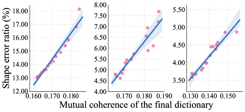
Figure 4: A scatter plot of the shape error ratio in percentage against the final dictionary coherence. A line is fitted based on the data. The left comes from subject 05, the middle from subject 18, the right from subject 64.

5.3.2 Missing data

Landmarks are not always visible from the camera owing to the occlusion by other objects or itself. In the present paper, we focus on a complete measurement situation not accounting for invisible landmarks. However, thanks to recent progress in matrix completion, our method can be easily extended to missing data. Moreover, in our experiments, we observe that deep neural network shows a well tolerance of missing data. Simply setting missing 2D coordinates as zeros provides satisfactory results. Such technique is widely used in deep-learning-based depth map reconstruction from sparse observations [9, 24, 21, 22, 7]. These two solutions make our central pipeline of DNN more easily to adapt to handling missing data.

5.4 Coherence as guide

As explained in Section 4.1, every sparse code $\boldsymbol{\psi}_{i}$ is constrained by its subsequent representation and thus the quality of code recovery depends less on the quality of the corresponding dictionary. However, this is not applicable to the final code $\boldsymbol{\psi}_{n}$, making it least constrained with the most dependency on the final dictionary $\mathbf{D}_{n}$. From this perspective, the quality of the final dictionary measured by mutual coherence [14] could serve as a lower bound of the entire system. To verify this, we compute the error and coherence in a fixed interval during training in NRSfM experiments. We consistently observe strong correlations between 3D reconstruction error and the mutual coherence of the final dictionary. We plot this relationship in Figure 4. We thus propose to use the coherence of the final dictionary as a measure of model quality for guiding training to efficiently avoid over-fitting especially when 3D evaluation is not available. This improves the utility of our deep NRSfM in future applications without 3D ground-truth.

6 Conclusion

In this paper, we proposed multi-layer sparse coding as a novel prior assumption for representing 3D non-rigid shapes and designed an innovative encoder-decoder neural network to solve the problem of NRSfM using no 3D supervision. The proposed network was derived by generalizing the classical sparse coding algorithm ISTA to a block sparse scenario. The proposed network architecture is mathematically interpretable as solving a NRSfM multi-layer sparse dictionary learning problem. Extensive experiments demonstrated our superior performance against the state-of-the-art methods and our generalization to unseen data. Finally, we proposed to use the coherence of the final dictionary as a model quality measure, offering a practical way to avoid over-fitting and select the best checkpoint during training without relying on 3D ground-truth.

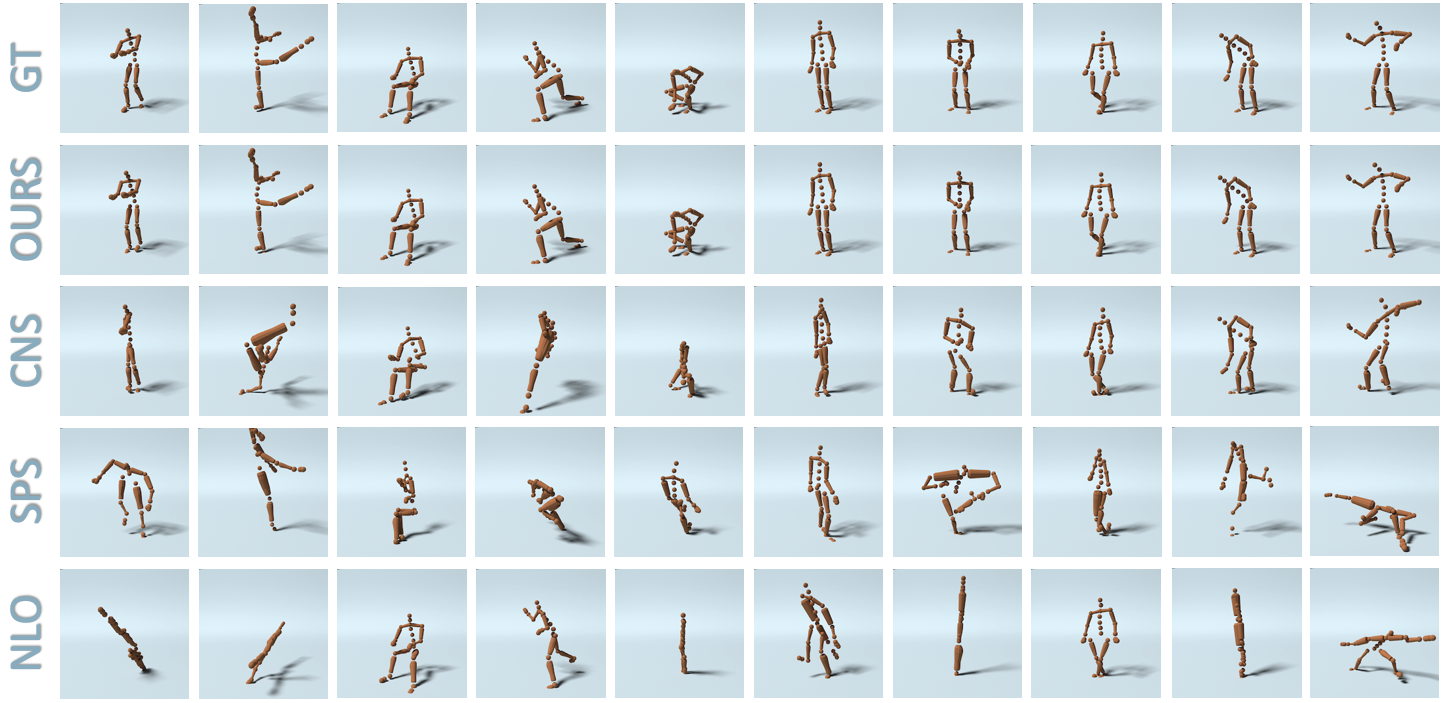
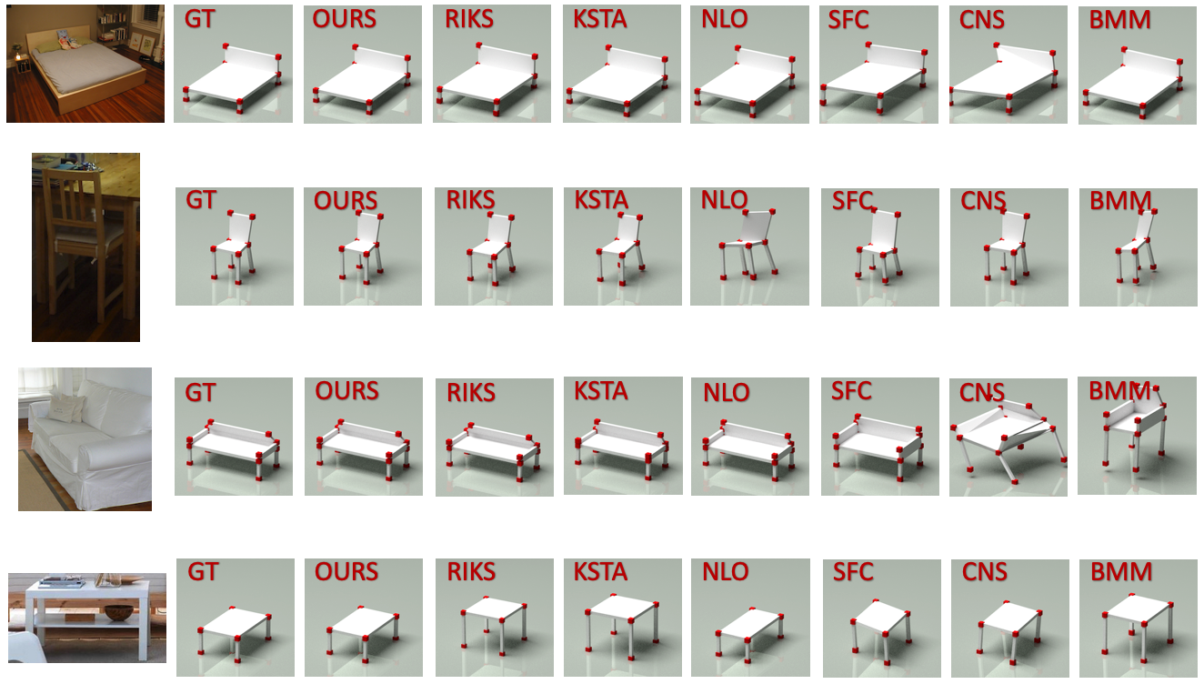
Figure 5: Qualitative evaluation on CMU Mocap dataset. Top to bottom: ground-truth, ours, CNS [20], SPS [18], NLO [12]. Each column corresponds to reconstructions of a certain frame, randomly selected from each subject. Spheres are reconstructed landmarks while bars are for visualization. 3D shapes are already aligned to the ground truth by orthonormal matrix.

Figure 6: Qualitative evaluation on IKEA dataset. Landmarks projected by annotated cameras are omitted from images. In each rendering, red cubes are reconstructed points while the planes and bars are manually added for descent visualization. Left to right: annotated image, ground-truth, ours, RIKS [17], KSTA [16], NLO [12], SFC [19], CNS [20], BMM [10].

References

- [1] Antonio Agudo and Francesc Moreno-Noguer. Dust: Dual union of spatio-temporal subspaces for monocular multiple object 3d reconstruction. In Proceedings of the IEEE Conference on Computer Vision and Pattern Recognition, pages 6262–6270, 2017.
- [2] Antonio Agudo, Melcior Pijoan, and Francesc Moreno-Noguer. Image collection pop-up: 3d reconstruction and clustering of rigid and non-rigid categories. In Proceedings of the IEEE Conference on Computer Vision and Pattern Recognition, pages 2607–2615, 2018.
- [3] Ijaz Akhter, Yaser Sheikh, and Sohaib Khan. In defense of orthonormality constraints for nonrigid structure from motion. In Computer Vision and Pattern Recognition, 2009. CVPR 2009. IEEE Conference on, pages 1534–1541. IEEE, 2009.
- [4] Ijaz Akhter, Yaser Sheikh, Sohaib Khan, and Takeo Kanade. Nonrigid structure from motion in trajectory space. In Advances in neural information processing systems, pages 41–48, 2009.
- [5] Amir Beck and Marc Teboulle. A fast iterative shrinkage-thresholding algorithm with application to wavelet-based image deblurring. In Acoustics, Speech and Signal Processing, 2009. ICASSP 2009. IEEE International Conference on, pages 693–696. IEEE, 2009.
- [6] Christoph Bregler, Aaron Hertzmann, and Henning Biermann. Recovering non-rigid 3d shape from image streams. In Computer Vision and Pattern Recognition, 2000. Proceedings. IEEE Conference on, volume 2, pages 690–696. IEEE, 2000.
- [7] Cesar Cadena, Anthony R Dick, and Ian D Reid. Multi-modal auto-encoders as joint estimators for robotics scene understanding. In Robotics: Science and Systems, 2016.
- [8] Angel X. Chang, Thomas A. Funkhouser, Leonidas J. Guibas, Pat Hanrahan, Qi-Xing Huang, Zimo Li, Silvio Savarese, Manolis Savva, Shuran Song, Hao Su, Jianxiong Xiao, Li Yi, and Fisher Yu. Shapenet: An information-rich 3d model repository. CoRR, abs/1512.03012, 2015.
- [9] Zhao Chen, Vijay Badrinarayanan, Gilad Drozdov, and Andrew Rabinovich. Estimating depth from rgb and sparse sensing. European Conference on Computer Vision (ECCV), 2018.
- [10] Yuchao Dai, Hongdong Li, and Mingyi He. A simple prior-free method for non-rigid structure-from-motion factorization. International Journal of Computer Vision, 107(2):101–122, 2014.
- [11] Ingrid Daubechies, Michel Defrise, and Christine De Mol. An iterative thresholding algorithm for linear inverse problems with a sparsity constraint. Communications on Pure and Applied Mathematics: A Journal Issued by the Courant Institute of Mathematical Sciences, 57(11):1413–1457, 2004.
- [12] Alessio Del Bue, Fabrizio Smeraldi, and Lourdes Agapito. Non-rigid structure from motion using ranklet-based tracking and non-linear optimization. Image and Vision Computing, 25(3):297–310, 2007.
- [13] Wei Deng, Wotao Yin, and Yin Zhang. Group sparse optimization by alternating direction method. In SPIE Optical Engineering+ Applications, pages 88580R–88580R. International Society for Optics and Photonics, 2013.
- [14] David L Donoho, Michael Elad, and Vladimir N Temlyakov. Stable recovery of sparse overcomplete representations in the presence of noise. IEEE Transactions on information theory, 52(1):6–18, 2006.
- [15] Katerina Fragkiadaki, Marta Salas, Pablo Arbelaez, and Jitendra Malik. Grouping-based low-rank trajectory completion and 3d reconstruction. In Advances in Neural Information Processing Systems, pages 55–63, 2014.
- [16] Paulo FU Gotardo and Aleix M Martinez. Kernel non-rigid structure from motion. In Computer Vision (ICCV), 2011 IEEE International Conference on, pages 802–809. IEEE, 2011.
- [17] Onur C Hamsici, Paulo FU Gotardo, and Aleix M Martinez. Learning spatially-smooth mappings in non-rigid structure from motion. In European Conference on Computer Vision, pages 260–273. Springer, 2012.
- [18] Chen Kong and Simon Lucey. Prior-less compressible structure from motion. Computer Vision and Pattern Recognition (CVPR), 2016.
- [19] Chen Kong, Rui Zhu, Hamed Kiani, and Simon Lucey. Structure from category: a generic and prior-less approach. International Conference on 3DVision (3DV), 2016.
- [20] Minsik Lee, Jungchan Cho, and Songhwai Oh. Consensus of non-rigid reconstructions. In Proceedings of the IEEE Conference on Computer Vision and Pattern Recognition, pages 4670–4678, 2016.
- [21] Yaoxin Li, Keyuan Qian, Tao Huang, and Jingkun Zhou. Depth estimation from monocular image and coarse depth points based on conditional gan. In MATEC Web of Conferences, volume 175, page 03055. EDP Sciences, 2018.
- [22] Yiyi Liao, Lichao Huang, Yue Wang, Sarath Kodagoda, Yinan Yu, and Yong Liu. Parse geometry from a line: Monocular depth estimation with partial laser observation. In Robotics and Automation (ICRA), 2017 IEEE International Conference on, pages 5059–5066. IEEE, 2017.
- [23] Joseph J. Lim, Hamed Pirsiavash, and Antonio Torralba. Parsing IKEA Objects: Fine Pose Estimation. ICCV, 2013.
- [24] Fangchang Mal and Sertac Karaman. Sparse-to-dense: Depth prediction from sparse depth samples and a single image. In 2018 IEEE International Conference on Robotics and Automation (ICRA), pages 1–8. IEEE, 2018.
- [25] Vardan Papyan, Yaniv Romano, and Michael Elad. Convolutional neural networks analyzed via convolutional sparse coding. The Journal of Machine Learning Research, 18(1):2887–2938, 2017.
- [26] Christopher J Rozell, Don H Johnson, Richard G Baraniuk, and Bruno A Olshausen. Sparse coding via thresholding and local competition in neural circuits. Neural computation, 20(10):2526–2563, 2008.
- [27] Hao Su, Charles R Qi, Yangyan Li, and Leonidas J Guibas. Render for cnn: Viewpoint estimation in images using cnns trained with rendered 3d model views. In Proceedings of the IEEE International Conference on Computer Vision, pages 2686–2694, 2015.
- [28] Jeremias Sulam, Vardan Papyan, Yaniv Romano, and Michael Elad. Multi-layer convolutional sparse modeling: Pursuit and dictionary learning. arXiv preprint arXiv:1708.08705, 2017.
- [29] Carlo Tomasi and Takeo Kanade. Shape and motion from image streams under orthography: a factorization method. International Journal of Computer Vision, 9(2):137–154, 1992.
- [30] Sara Vicente, João Carreira, Lourdes Agapito, and Jorge Batista. Reconstructing pascal voc. In 2014 IEEE Conference on Computer Vision and Pattern Recognition, pages 41–48. IEEE, 2014.
- [31] Jiajun Wu, Tianfan Xue, Joseph J Lim, Yuandong Tian, Joshua B Tenenbaum, Antonio Torralba, and William T Freeman. Single image 3d interpreter network. European Conference on Computer Vision (ECCV), 2016.
- [32] Zhirong Wu, Shuran Song, Aditya Khosla, Fisher Yu, Linguang Zhang, Xiaoou Tang, and Jianxiong Xiao. 3d shapenets: A deep representation for volumetric shapes. In Proceedings of the IEEE conference on computer vision and pattern recognition, pages 1912–1920, 2015.
- [33] Yu Xiang, Roozbeh Mottaghi, and Silvio Savarese. Beyond pascal: A benchmark for 3d object detection in the wild. In IEEE Winter Conference on Applications of Computer Vision, pages 75–82. IEEE, 2014.
- [34] Xiaowei Zhou, Spyridon Leonardos, Xiaoyan Hu, and Kostas Daniilidis. 3d shape estimation from 2d landmarks: A convex relaxation approach. In Proceedings of the IEEE Conference on Computer Vision and Pattern Recognition, pages 4447–4455, 2015.
- [35] Xiaowei Zhou, Menglong Zhu, Spyridon Leonardos, Kosta Derpanis, and Kostas Daniilidis. Sparseness meets deepness: 3d human pose estimation from monocular video. arXiv preprint arXiv:1511.09439, 2015.
- [36] Yingying Zhu, Dong Huang, Fernando De La Torre, and Simon Lucey. Complex non-rigid motion 3d reconstruction by union of subspaces. In Computer Vision and Pattern Recognition (CVPR), 2014 IEEE Conference on, pages 1542–1549. IEEE, 2014.
- [37] Yingying Zhu and Simon Lucey. Convolutional sparse coding for trajectory reconstruction. Pattern Analysis and Machine Intelligence, IEEE Transactions on, 37(3):529–540, 2015.