On Mutual Information Maximization for Representation Learning
Abstract
Many recent methods for unsupervised or self-supervised representation learning train feature extractors by maximizing an estimate of the mutual information (MI) between different views of the data. This comes with several immediate problems: For example, MI is notoriously hard to estimate, and using it as an objective for representation learning may lead to highly entangled representations due to its invariance under arbitrary invertible transformations. Nevertheless, these methods have been repeatedly shown to excel in practice. In this paper we argue, and provide empirical evidence, that the success of these methods cannot be attributed to the properties of MI alone, and that they strongly depend on the inductive bias in both the choice of feature extractor architectures and the parametrization of the employed MI estimators. Finally, we establish a connection to deep metric learning and argue that this interpretation may be a plausible explanation for the success of the recently introduced methods.
1 Introduction
Unsupervised representation learning is a fundamental problem in machine learning. Intuitively, one aims to learn a function which maps the data into some, usually lower-dimensional, space where one can solve some (generally a priori unknown) target supervised tasks more efficiently, i.e. with fewer labels. In contrast to supervised and semi-supervised learning, the learner has access only to unlabeled data. Even though the task seems ill-posed as there is no natural objective one should optimize, by leveraging domain knowledge this approach can be successfully applied to a variety of problem areas, including image (Kolesnikov et al., 2019; van den Oord et al., 2018; Hénaff et al., 2019; Tian et al., 2019; Hjelm et al., 2019; Bachman et al., 2019) and video classification (Wang and Gupta, 2015; Sun et al., 2019), and natural language understanding (van den Oord et al., 2018; Peters et al., 2018; Devlin et al., 2019).
Recently, there has been a revival of approaches inspired by the InfoMax principle (Linsker, 1988): Choose a representation maximizing the mutual information (MI) between the input and its representation, possibly subject to some structural constraints. MI measures the amount of information obtained about a random variable by observing some other random variable 111We denote random variables using upper-case letters (e.g. , ), and their realizations by the corresponding lower-case letter (e.g. , ). Formally, the MI between and , with joint density and marginal densities and , is defined as the Kullback–Leibler (KL) divergence between the joint and the product of the marginals
| (1) |
The fundamental properties of MI are well understood and have been extensively studied (see e.g. Kraskov et al. (2004)). Firstly, MI is invariant under reparametrization of the variables — namely, if and are homeomorphisms (i.e. smooth invertible maps), then . Secondly, estimating MI in high-dimensional spaces is a notoriously difficult task, and in practice one often maximizes a tractable lower bound on this quantity (Poole et al., 2019). Nonetheless, any distribution-free high-confidence lower bound on entropy requires a sample size exponential in the size of the bound (McAllester and Statos, 2018).
Despite these fundamental challenges, several recent works have demonstrated promising empirical results in representation learning using MI maximization (van den Oord et al., 2018; Hénaff et al., 2019; Tian et al., 2019; Hjelm et al., 2019; Bachman et al., 2019; Sun et al., 2019). In this work we argue, and provide empirical evidence, that the success of these methods cannot be attributed to the properties of MI alone. In fact, we show that maximizing tighter bounds on MI can result in worse representations. In addition, we establish a connection to deep metric learning and argue that this interpretation may be a plausible explanation of the success of the recently introduced methods.222The code for running the experiments and visualizing the results is available at https://github.com/google-research/google-research/tree/master/mutual_information_representation_learning.
2 Background and Related Work
Recent progress and the InfoMax principle While promising results in other domains have been presented in the literature, we will focus on unsupervised image representation learning techniques that have achieved state-of-the-art performance on image classification tasks (Hénaff et al., 2019; Tian et al., 2019; Bachman et al., 2019). The usual problem setup dates back at least to Becker and Hinton (1992) and can conceptually be described as follows: For a given image , let and be different, possibly overlapping views of , for instance the top and bottom halves of the image. These are encoded using encoders and respectively, and the MI between the two representations and is maximized,
| (2) |
where is a sample-based estimator of the true MI and the function classes and can be used to specify structural constraints on the encoders. While not explicitly reflected in (2), note that and can often share parameters. Furthermore, it can be shown that ,333Follows from the data processing inequality (see Prop. 1 in Appendix A). hence the objective in (2) can be seen as a lower bound on the InfoMax objective (Linsker, 1988).
Practical advantages of multi-view formulations There are two main advantages in using (2) rather than the original InfoMax objective. First, the MI has to be estimated only between the learned representations of the two views, which typically lie on a much lower-dimensional space than the one where the original data lives. Second, it gives us plenty of modeling flexibility, as the two views can be chosen to capture completely different aspects and modalities of the data, for example:
-
1.
In the basic form of DeepInfoMax (Hjelm et al., 2019) extracts global features from the entire image and local features from image patches , where and correspond to activations in different layers of the same convolutional network. Bachman et al. (2019) build on this and compute the two views from different augmentations of the same image.
- 2.
-
3.
Contrastive predictive coding (CPC) (van den Oord et al., 2018; Hénaff et al., 2019) incorporates a sequential component of the data. Concretely, one extracts a sequence of patches from an image in some fixed order, maps each patch using an encoder, aggregates the resulting features of the first patches into a context vector, and maximizes the MI between the context and features extracted from the patch at position . In (2), would thus correspond to the first patches and to the patch at location .
Other approaches, such as those presented by Sermanet et al. (2018), Hu et al. (2017), and Ji et al. (2019), can be similarly subsumed under the same objective.
Lower bounds on MI As evident from (2), another critical choice is the MI estimator . Given the fundamental limitations of MI estimation (McAllester and Statos, 2018), recent work has focused on deriving lower bounds on MI (Barber and Agakov, 2003; Belghazi et al., 2018; Poole et al., 2019). Intuitively, these bounds are based on the following idea: If a classifier can accurately distinguish between samples drawn from the joint and those drawn from the product of marginals , then and have a high MI.
We will focus on two such estimators, which are most commonly used in the representation learning literature. The first of them, termed InfoNCE (van den Oord et al., 2018), is defined as
| (3) |
where the expectation is over independent samples from the joint distribution (Poole et al., 2019). In practice we estimate (3) using Monte Carlo estimation by averaging over multiple batches of samples. Intuitively, the critic function tries to predict for each which of the samples it was jointly drawn with, by assigning high values to the jointly drawn pair, and low values to all other pairs. The second estimator is based on the variational form of the KL divergence due to Nguyen, Wainwright, and Jordan (NWJ) (Nguyen et al., 2010) and takes the form
| (4) |
For detailed derivations we refer the reader to (Ruderman et al., 2012; Poole et al., 2019). Note that these bounds hold for any critic and when used in (2) one in practice jointly maximizes over and . Furthermore, it can be shown that (3) is maximized by and (4) by (Poole et al., 2019). Common choices for include bilinear critics (van den Oord et al., 2018; Hénaff et al., 2019; Tian et al., 2019), separable critics (Bachman et al., 2019), and concatenated critics (Hjelm et al., 2019) (here are typically shallow multi-layer perceptrons (MLPs)). When applying these estimators to solve (2), the line between the critic and the encoders can be blurry. For example, one can train with an inner product critic , but extract features from an intermediate layer of , in which case the top layers of form a separable critic. Nevertheless, this boundary is crucial for the interplay between MI estimation and the interpretation of the learned representations.
3 Biases in approximate information maximization
It is folklore knowledge that maximizing MI does not necessarily lead to useful representations. Already Linsker (1988) talks in his seminal work about constraints, while a manifestation of the problem in clustering approaches using MI criteria has been brought up by Bridle et al. (1992) and subsequently addressed using regularization by Krause et al. (2010). To what can we then attribute the recent success of methods building on the principles of MI maximization? We will argue that their connection to the InfoMax principle might be very loose. Namely, we will show that they behave counter-intuitively if one equates them with MI maximization, and that the performance of these methods depends strongly on the bias that is encoded not only in the encoders, but also on the actual form of the used estimators.
-
1.
We first consider encoders which are bijective by design. Even though the true MI is maximized for any choice of model parameters, the representation quality (measured by downstream linear classification accuracy) improves during training. Furthermore, there exist invertible encoders for which the representation quality is worse than using raw pixels, despite also maximizing MI.
-
2.
We next consider encoders that can model both invertible and non-invertible functions. When the encoder can be non-invertible, but is initialized to be invertible, still biases the encoders to be very ill-conditioned and hard to invert.
-
3.
For and , higher-capacity critics admit tighter bounds on MI. We demonstrate that simple critics yielding loose bounds can lead to better representations than high-capacity critics.
-
4.
Finally, we optimize the estimators to the same MI lower-bound value with different encoder architectures and show that the representation quality can be impacted more by the choice of the architecture, than the estimator.
As a consequence, we argue that the success of these methods and the way they are instantiated in practice is only loosely connected to MI. Then, in Section 4 we provide an alternative explanation for the success of recent methods through a connection to classic triplet losses from metric learning.
Setup Our goal is to provide a minimal set of easily reproducible empirical experiments to understand the role of MI estimators, critic and encoder architectures when learning representations via the objective (2). To this end, we consider a simple setup of learning a representation of the top half of MNIST handwritten digit images (we present results for the experiments from Sections 3.2 and 3.3 on CIFAR10 in Appendix G; the conclusions are analogous). This setup has been used in the context of deep canonical correlation analysis (Andrew et al., 2013), where the target is to maximize the correlation between the representations. Following the widely adopted downstream linear evaluation protocol (Kolesnikov et al., 2019; van den Oord et al., 2018; Hénaff et al., 2019; Tian et al., 2019; Hjelm et al., 2019; Bachman et al., 2019), we train a linear classifier444Using SAGA (Defazio et al., 2014), as implemented in scikit-learn (Pedregosa et al., 2011). for digit classification on the learned representation using all available training labels (other evaluation protocols are discussed in Section 5). To learn the representation we instantiate (2) and split each input MNIST image into two parts, the top part of the image corresponding to , and the bottom part, , corresponding to , respectively. We train , , and using the Adam optimizer (Kingma and Ba, 2015), and use as the representation for the linear evaluation. Unless stated otherwise, we use a bilinear critic (we investigate its effect in a separate ablation study), set the batch size to and the learning rate to .555Note that is upper-bounded by (van den Oord et al., 2018). We experimented with batch sizes up to and obtained consistent results aligned with the stated conclusions. Throughout, values and downstream classification accuracies are averaged over runs and reported on the testing set (we did not observe large gaps between the training and testing values of ). As a common baseline, we rely on a linear classifier in pixel space on , which obtains a testing accuracy of about . For comparison, a simple MLP or ConvNet architecture achieves about (see Section 3.3 for details).
3.1 Large MI is not predictive of downstream performance
We start by investigating the behavior of and when and are parameterized to be always invertible. Hence, for any choice of the encoder parameters, the MI is constant, i.e. for all . This means that if we could exactly compute the MI, any parameter choice would be a global maximizer and thus the gradients vanish everywhere.666In the context of continuous distributions and invertible representation functions the InfoMax objective might be infinite. Bell and Sejnowski (1995) suggest to instead maximize the entropy of the representation. In our case the MI between the two views is finite as the two halves are not deterministic functions of each another. However, as we will empirically show, the estimators we consider are biased and prefer those settings which yield representations useful for the downstream classification task.
Maximized MI and improved downstream performance We model and using the invertible RealNVP architecture (Dinh et al., 2016). We use a total of 30 coupling layers, and each of them computes the shift using a separate MLP with two ReLU hidden layers, each with 512 units.
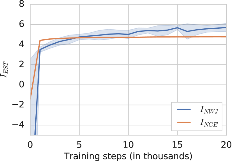
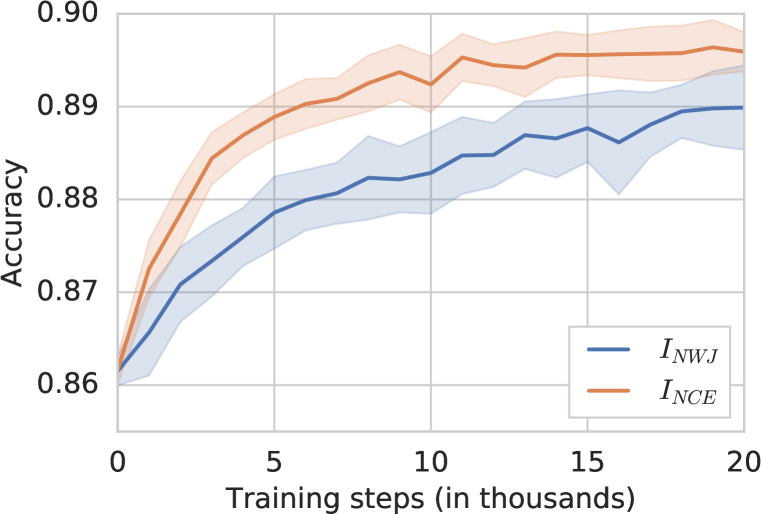
Figure 1 shows the testing value of and the testing accuracy on the classification task. Despite the fact that MI is maximized by any instantiation of and , and downstream accuracy increase during training, implying that the estimators provide gradient feedback leading to a representation useful for linear classification. This confirms our hypothesis that the estimator biases the encoders towards solutions suitable to solve the downstream linear classification task.
The previous experiment demonstrated that among many invertible encoders, all of which are globally optimal MI maximizers, some give rise to improved linear classification performance over raw pixels, and maximizing and yields such encoders. Next we demonstrate that for the same invertible encoder architecture there are model parameters for which linear classification performance is significantly worse than using raw pixels, despite also being globally optimal MI maximizers.
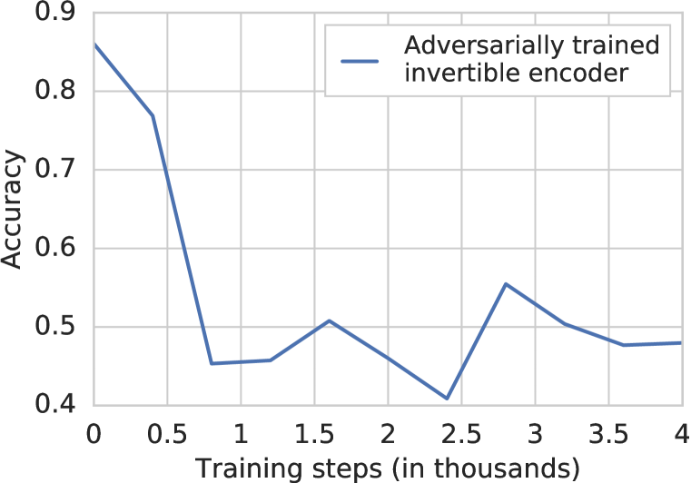
Maximized MI and worsened downstream performance The goal is to learn a (bijective) representation maximizing MI such that the optimal linear classifier performs poorly; we achieve this by jointly training a representation and classifier in an adversarial fashion (a separate classifier is trained for the evaluation), without using a MI estimator. Intuitively, we will train the encoder to make the classification task for the linear layer as hard as possible. The experimental details are presented in Appendix B. Figure 1(c) shows the result of one such training run, displaying the loss of a separately trained classifier on top of the frozen representation. At the beginning of training the network is initialized to be close to the identity mapping, and as such achieves the baseline classification accuracy corresponding to raw pixels. All points beyond this correspond to invertible feature maps with worse classification performance, despite still achieving globally maximal MI.
Alternatively, the following thought experiment would yield the same conclusion: Using a lossless compression algorithm (e.g. PNG) for and also satisfies . Yet, performing linear classification on the raw compressed bit stream will likely lead to worse performance than the baseline in pixel space. The information content alone is not sufficient to guarantee a useful geometry in the representation space.
We next investigate the behavior of the model if we use a network architecture that can model both invertible and non-invertible functions. We would like to understand whether prefers the network to remain bijective, thus maximizing the true MI, or to ignore part of the input signal, which can be beneficial for representation learning.
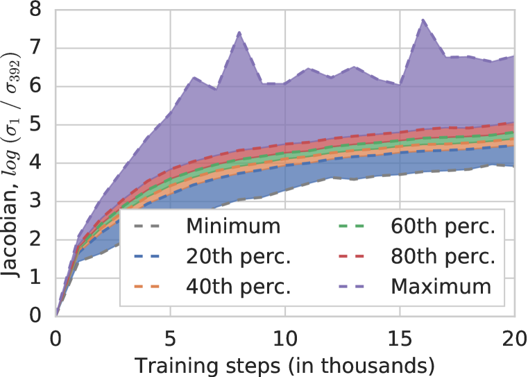
Bias towards hard-to-invert encoders We use an MLP architecture with hidden layers of the same dimension as the input, and with a skip connection added to each layer (hence by setting all weights to the network becomes the identity function). As quantifying invertibility is hard, we analyze the condition number, i.e. the ratio between the largest and the smallest singular value, of the Jacobian of : By the implicit function theorem, the function is invertible if the Jacobian is non-singular.777Formally, is invertible as long as the condition number of the Jacobian is finite. Numerically, inversion becomes harder as the condition number increases. However, the data itself might lie on a low-dimensional manifold, so that having a singular Jacobian is not necessarily indicative of losing invertibility on the support of the data distribution. To ensure the support of the data distribution covers the complete input space, we corrupt and in a coupled way by adding to each the same 392-dimensional random vector, whose coordinates are sampled (independently of ) from a normal with standard deviation (the standard deviation of the pixels themselves is 0.3). Hence, non-invertible encoders do not maximize . 888This would not necessarily be true if the noise were added in an uncoupled manner, e.g. by drawing it independently for and , as the MI between the two noise vectors is in that case. As a reference point, the linear classification accuracy from pixels drops to about 84% due to the added noise.
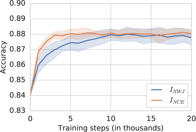
In Figure 2 we can see that the value and the downstream accuracy both increase during training, as before. Moreover, even though is initialized very close to the identity function (which maximizes the true MI), the condition number of its Jacobian evaluated at inputs randomly sampled from the data-distribution steadily deteriorates over time, suggesting that in practice (i.e. numerically) inverting the model becomes increasingly hard. It therefore seems that the bounds we consider favor hard-to-invert encoders, which heavily attenuate part of the noise (as the support of the noise is the entire input space), over well conditioned encoders (such as the identity function at initialization), which preserve the noise and hence the entropy of the data well.
3.2 Higher capacity critics can lead to worse downstream performance
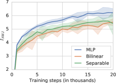
In the previous section we have established that MI and downstream performance are only loosely connected. Clearly, maximizing MI is not sufficient to learn good representations and there is a non-trivial interplay between the architectures of the encoder, critic, and the underlying estimators. In this section, we will focus on how one of these factors, namely the critic architecture, impacts the quality of the learned representation. Recall that it determines how the estimators such as and distinguish between samples from the joint distribution and the product of the marginals , and thereby determines the tightness on the lower bound. A higher capacity critic should allow for a tighter lower-bound on MI (Belghazi et al., 2018). Furthermore, in the context of representation learning where is instantiated as a neural network, the critic provides gradient feedback to and and thereby shapes the learned representation.
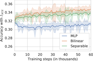
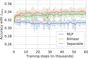
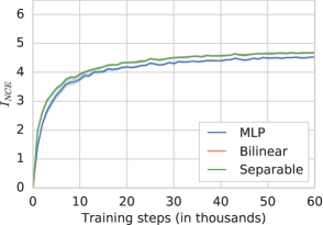
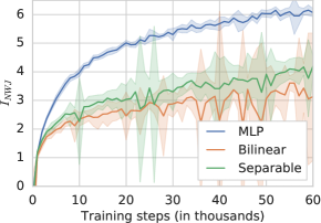
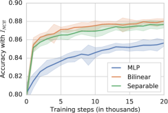
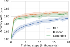
Looser bounds with simpler critics can lead to better representations We compare three critic architectures, a bilinear critic, a separable critic ( are MLPs with a single hidden layer with units and ReLU activations, followed by a linear layer with units; comprising k parameters in total) and an MLP critic with a single hidden layer with units and ReLU activations, applied to the concatenated input (k trainable parameters). Further, we use identical MLP architectures for and with two hidden layers comprising units each, and a third linear layer mapping to a -dimensional feature space.
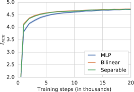
Figure 3 shows the downstream testing accuracy and the testing value as a function of the iteration (see Appendix G for the corresponding results on CIFAR10). It can be seen that for both lower bounds, representations trained with the MLP critic barely outperform the baseline on pixel space, whereas the same lower bounds with bilinear and separable critics clearly lead to a higher accuracy than the baseline. While the testing value is close to the theoretically achievable maximum value for all critics, the testing value is higher for the MLP critic than for the separable and bilinear critics, resulting in a tighter bound on the MI. However, despite achieving the smallest testing value, the simple bilinear critic leads to a better downstream performance than the higher-capacity separable and MLP critics.
3.3 Encoder architecture can be more important than the specific estimator
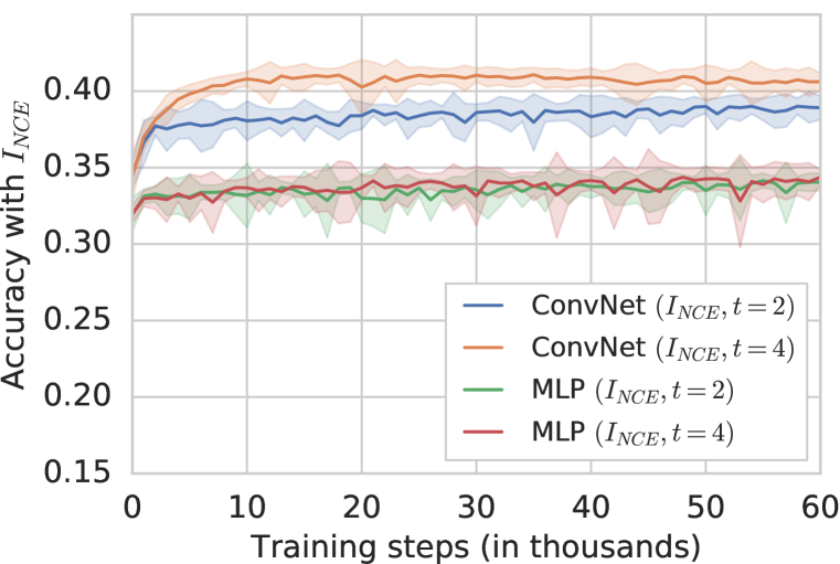
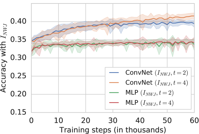
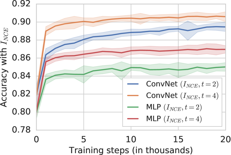
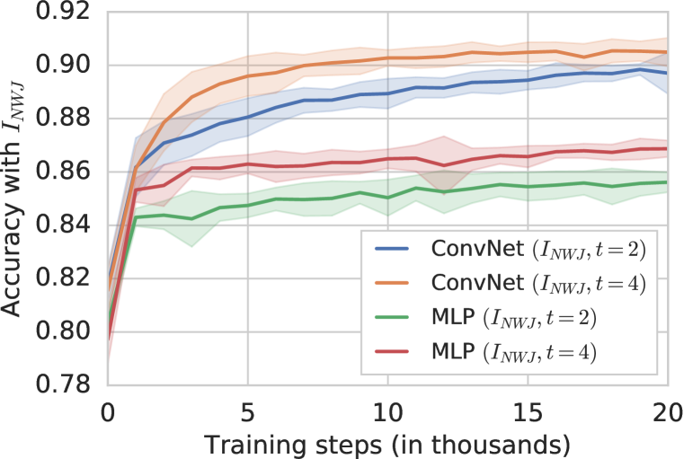
We will now show that the encoder architecture is a critical design choice and we will investigate its effect on the learned representation. We consider the same MLP architecture (k parameters) as in Section 3.2, as well as a ConvNet architecture comprising two convolution layers (with a kernel, stride of , ReLU activations, and and channels, respectively; k parameters), followed by spatial average pooling and a fully connected layer. Before the average pooling operation we apply layer normalization (Ba et al., 2016) which greatly reduces the variance of .999LayerNorm avoids the possibility of information leakage within mini-batches that can be induced through batch normalization, potentially leading to poor performance (Hénaff et al., 2019). To ensure that both network architectures achieve the same lower bound on the MI, we minimize instead of solving (2), for two different values .
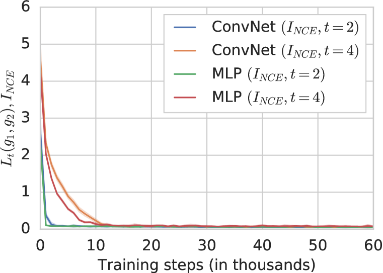
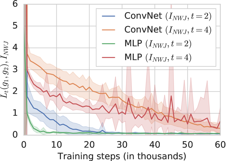
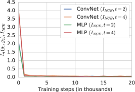
Figure 4 shows the downstream testing accuracy as a function of the training iteration (see Appendix G for the corresponding results on CIFAR10). It can be seen in the testing loss curves in Appendix F that for both architectures and estimators the objective value after k iterations matches the target (i.e., ) which implies that they achieve the same lower-bound on the MI. Despite matching lower bounds, ConvNet encoders lead to clearly superior classification accuracy, for both and . Note that, in contrast, the MLP and ConvNet architectures trained end-to-end in supervised fashion both achieve essentially the same testing accuracy of about .
In the context of VAEs, Alemi et al. (2018) similarly observed that models achieving the same evidence lower bound value can lead to vastly different representations depending on the employed encoder architecture, and do not necessarily capture useful information about the data (Tschannen et al., 2018; Blau and Michaeli, 2019).
4 Connection to deep metric learning and triplet losses
In the previous section we empirically demonstrated that there is a disconnect between approximate MI maximization and representation quality. However, many recent works have applied the estimator to obtain state-of-the-art results in practice. We provide some insight on this conundrum by connecting to a popular triplet (-plet) loss known in the deep metric learning community.
The metric learning view Given sets of triplets, namely an anchor point , a positive instance , and a negative instance , the goal is to learn a representation such that the distances (i.e., ) between and is smaller than the distance between and , for each triplet. In the supervised setting, the positive instances are usually sampled from the same class, while the negative instances are sampled from any other class. A major focus in deep metric learning is how to perform (semi-)hard positive mining — we want to present non-trivial triplets to the learning algorithm which become more challenging as improves. Natural extensions to the unsupervised setting can be obtained by exploiting the structure present in the input data, namely spatial (e.g. patches from the same image should be closer than patches from different images) and temporal information (temporally close video frames should be encoded closer than the ones which are further away in time) (Hoffer and Ailon, 2015).
Connection to InfoNCE The InfoNCE objective can be rewritten as follows:
The derivation is presented in Appendix C. In the particular case that and take value in the same space and is constrained to be of the form , for some function , this coincides (up to constants and change of sign) with the expectation of the multi-class K-pair loss proposed in (Sohn, 2016, Eqn. (7)):
| (5) |
Representation learning by maximizing using a symmetric separable critic and an encoder shared across views is thus equivalent to metric learning based on (5). When using different encoders for different views and asymmetric critics as employed by CPC, DeepInfoMax, and CMC one recovers asymmetric variants of (5), see, e.g. (Yu et al., 2017; Zhang et al., 2019). As a result, one can view (5) as learning encoders with a parameter-less inner product critic, for which the MI lower-bound is very weak in general.
There are (at least) two immediate benefits of viewing recent representation learning methods based on MI estimators through the lens of metric learning. Firstly, in the MI view, using inner product or bilinear critic functions is sub-optimal since the critic should ideally be as flexible as possible in order to reduce the gap between the lower bound and the true MI. In the metric learning view, the inner product critic corresponds to a simple metric on the embedding space. The metric learning view seems hence in better accordance with the observations from Section 3.2 than the MI view. Secondly, it elucidates the importance of appropriately choosing the negative samples, which is indeed a critical component in deep metric learning based on triplet losses (Norouzi et al., 2012; Schroff et al., 2015).
InfoNCE and the importance of negative sampling The negative sample mining issue also manifests itself in MI-based contrastive losses. In fact, while InfoNCE is a lower bound on MI if the negative samples are drawn from the true marginal distribution (Poole et al., 2019), i.e.
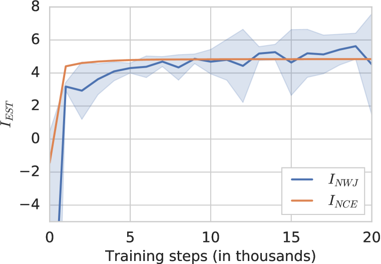
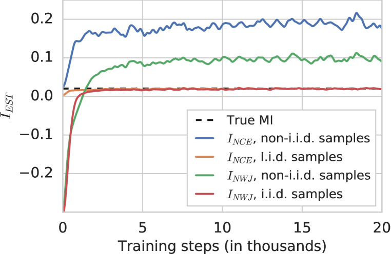
we show that if the negative samples are drawn in a dependent fashion (corresponding to the being drawn identically but not independently), the estimator is in general neither a lower nor an upper bound on the true MI . We prove this in Appendix D and present empirical evidence here. Let , where and are two-dimensional Gaussians. We generate batches of data where each is sampled independently for each element of the batch, but is sampled only once per batch. As such, has the same marginal distribution for each , but the elements of the batch are not independent. Although we do not treat it theoretically, we also display results of the same experiment using the estimator. The experimental details are presented in Appendix E. We observe in Figure 4c that when using non-i.i.d. samples both the and values are larger than the true MI, and that when i.i.d. samples are used, both are lower bounds on the true MI. Hence, the connection to MI under improper negative sampling is no longer clear and might vanish completely.
Notwithstanding this fundamental problem, the negative sampling strategy is often treated as a design choice. In Hénaff et al. (2019), CPC is applied to images by partitioning the input image into patches. Then, MI (estimated by InfoNCE) between representations of patches and a context summarizing several patches that are vertically above or below in the same image is minimized. Negative samples are obtained by patches from different images as well as patches from the same image, violating the independence assumption. Similarly, van den Oord et al. (2018) learn representations of speech using samples from a variety of speakers. It was found that using utterances from the same speaker as negative samples is more effective, whereas the “proper” negative samples should be drawn from an appropriate mixture of utterances from all speakers.
A common observation is that increasing the number of negative examples helps in practice (Hjelm et al., 2019; Tian et al., 2019; Bachman et al., 2019). Indeed, Ma and Collins (2018) show that is consistent for any number of negative samples (under technical conditions), and Poole et al. (2019) show that the signal-to-noise ratio increases with the number of negative samples. On the other hand, (Arora et al., 2019) have demonstrated, both theoretically and empirically, that increasing the number of negative samples does not necessarily help, and can even deteriorate the performance. The intricacies of negative sampling hence remain a key research challenge.
5 Conclusion
Is MI maximization a good objective for learning good representations in an unsupervised fashion? Possibly, but it is clearly not sufficient. In this work we have demonstrated that, under the common linear evaluation protocol, maximizing lower bounds on MI as done in modern incarnations of the InfoMax principle can result in bad representations. We have revealed that the commonly used estimators have strong inductive biases and—perhaps surprisingly—looser bounds can lead to better representations. Furthermore, we have demonstrated that the connection of recent approaches to MI maximization might vanish if negative samples are not drawn independently (as done by some approaches in the literature). As a result, it is unclear whether the connection to MI is a sufficient (or necessary) component for designing powerful unsupervised representation learning algorithms. We propose that the success of these recent methods could be explained through the view of triplet-based metric learning and that leveraging advances in that domain might lead to further improvements. We have several suggestions for future work, which we summarize in the following.
Alternative measures of information We believe that the question of developing new notions of information suitable for representation learning should receive more attention. While MI has appealing theoretical properties, it is clearly not sufficient for this task—it is hard to estimate, invariant to bijections and can result in suboptimal representations which do not correlate with downstream performance. Therefore, a new notion of information should account for both the amount of information stored in a representation and the geometry of the induced space necessary for good performance on downstream tasks. One possible avenue is to consider extensions to MI which explicitly account for the modeling power and computational constraints of the observer, such as the recently introduced -information Xu et al. (2020). Alternatively, one can investigate other statistical divergences to measure the discrepancy between and . For example, using the Wasserstein distance leads to promising results in representation learning as it naturally enforces smoothness in the encoders (Ozair et al., 2019).
A holistic view We believe that any theory on measuring information for representation learning built on critics should explicitly take into account the function families one uses (e.g. that of the critic and estimator). Most importantly, we would expect some natural trade-offs between the amount of information that can be stored against how hard it is to extract it in the downstream tasks as a function of the architectural choices. While the distribution of downstream tasks is typically assumed unknown in representation learning, it might be possible to rely on weaker assumptions such as a family of invariances relevant for the downstream tasks. Moreover, it seems that in the literature (i) the critics that are used to measure the information, (ii) the encoders, and (iii) the downstream models/evaluation protocol are all mostly chosen independently of each other. Our empirical results show that the downstream performance depends on the intricate balance between these choices and we believe that one should co-design them. This holistic view is currently under-explored and due to the lack of any theory or extensive studies to guide the practitioners.
Going beyond the widely used linear evaluation protocol While it was shown that learning good representations under the linear evaluation protocol can lead to reduced sample complexity for downstream tasks (Arora et al., 2019), some recent works (Bachman et al., 2019; Tian et al., 2019) report marginal improvements in terms of the downstream performance under a non-linear regime. Related to the previous point, it would hence be interesting to further explore the implications of the evaluation protocol, in particular its importance in the context of other design choices. We stress that a highly-nonlinear evaluation framework may result in better downstream performance, but it defeats the purpose of learning efficiently transferable data representations.
Systematic investigations into design decisions that matter On the practical side, we believe that the link to metric learning could lead to new methods, that break away from the goal of estimating MI and place more weight on the aspects that have a stronger effect on the performance such as the negative sampling strategy. An example where the metric learning perspective led to similar methods as the MI view is presented by Sermanet et al. (2018): They developed a multi-view representation learning approach for video data similar to CMC, but without drawing negative samples independently and seemingly without relying on the MI mental model to motivate their design choices.
Acknowledgments
We would like to thank Alex Alemi, Ben Poole, Olivier Bachem, and Alexey Dosovitskiy for inspiring discussions and comments on the manuscript. We are grateful for the general support and discussions from other members of Google Brain team in Zurich.
References
- Alemi et al. (2018) Alexander Alemi, Ben Poole, Ian Fischer, Joshua Dillon, Rif A Saurous, and Kevin Murphy. Fixing a Broken ELBO. In International Conference on Machine Learning, 2018.
- Andrew et al. (2013) Galen Andrew, Raman Arora, Jeff Bilmes, and Karen Livescu. Deep canonical correlation analysis. In International Conference on Machine Learning, 2013.
- Arora et al. (2019) Sanjeev Arora, Hrishikesh Khandeparkar, Mikhail Khodak, Orestis Plevrakis, and Nikunj Saunshi. A theoretical analysis of contrastive unsupervised representation learning. In International Conference on Machine Learning, 2019.
- Ba et al. (2016) Jimmy Lei Ba, Jamie Ryan Kiros, and Geoffrey E Hinton. Layer normalization. arXiv preprint arXiv:1607.06450, 2016.
- Bachman et al. (2019) Philip Bachman, R Devon Hjelm, and William Buchwalter. Learning representations by maximizing mutual information across views. In Advances in Neural Information Processing Systems, 2019.
- Barber and Agakov (2003) David Barber and Felix V Agakov. The IM algorithm: a variational approach to information maximization. In Advances in Neural Information Processing Systems, 2003.
- Becker and Hinton (1992) Suzanna Becker and Geoffrey E Hinton. Self-organizing neural network that discovers surfaces in random-dot stereograms. Nature, 1992.
- Belghazi et al. (2018) Mohamed Ishmael Belghazi, Aristide Baratin, Sai Rajeshwar, Sherjil Ozair, Yoshua Bengio, Devon Hjelm, and Aaron Courville. Mutual information neural estimation. In International Conference on Machine Learning, 2018.
- Bell and Sejnowski (1995) Anthony J Bell and Terrence J Sejnowski. An information-maximization approach to blind separation and blind deconvolution. Neural computation, 1995.
- Blau and Michaeli (2019) Yochai Blau and Tomer Michaeli. Rethinking lossy compression: The rate-distortion-perception tradeoff. In International Conference on Machine Learning, 2019.
- Bridle et al. (1992) John S Bridle, Anthony JR Heading, and David JC MacKay. Unsupervised classifiers, mutual information and phantom targets. In Advances in Neural Information Processing Systems, 1992.
- Defazio et al. (2014) Aaron Defazio, Francis Bach, and Simon Lacoste-Julien. SAGA: A fast incremental gradient method with support for non-strongly convex composite objectives. In Advances in Neural Information Processing Systems, 2014.
- Devlin et al. (2019) Jacob Devlin, Ming-Wei Chang, Kenton Lee, and Kristina Toutanova. BERT: Pre-training of deep bidirectional transformers for language understanding. In Conference of the North American Chapter of the Association for Computational Linguistics: Human Language Technologies, 2019.
- Dinh et al. (2016) Laurent Dinh, Jascha Sohl-Dickstein, and Samy Bengio. Density estimation using real nvp. arXiv preprint arXiv:1605.08803, 2016.
- Hénaff et al. (2019) Olivier J Hénaff, Ali Razavi, Carl Doersch, SM Eslami, and Aaron van den Oord. Data-efficient image recognition with contrastive predictive coding. arXiv preprint arXiv:1905.09272, 2019.
- Hjelm et al. (2019) R Devon Hjelm, Alex Fedorov, Samuel Lavoie-Marchildon, Karan Grewal, Phil Bachman, Adam Trischler, and Yoshua Bengio. Learning deep representations by mutual information estimation and maximization. In International Conference on Learning Representations, 2019.
- Hoffer and Ailon (2015) Elad Hoffer and Nir Ailon. Deep metric learning using triplet network. In International Workshop on Similarity-Based Pattern Recognition, 2015.
- Hu et al. (2017) Weihua Hu, Takeru Miyato, Seiya Tokui, Eiichi Matsumoto, and Masashi Sugiyama. Learning discrete representations via information maximizing self-augmented training. In International Conference on Machine Learning, 2017.
- Ji et al. (2019) Xu Ji, João F Henriques, and Andrea Vedaldi. Invariant information clustering for unsupervised image classification and segmentation. In IEEE International Conference on Computer Vision, 2019.
- Kingma and Ba (2015) Diederik P Kingma and Jimmy Ba. Adam: A method for stochastic optimization. International Conference on Learning Representation, 2015.
- Kingma and Welling (2014) Diederik P Kingma and Max Welling. Auto-encoding variational Bayes. International Conference on Learning Representation, 2014.
- Kolesnikov et al. (2019) Alexander Kolesnikov, Xiaohua Zhai, and Lucas Beyer. Revisiting self-supervised visual representation learning. International Conference on Computer Vision, 2019.
- Kraskov et al. (2004) Alexander Kraskov, Harald Stögbauer, and Peter Grassberger. Estimating mutual information. Physical review E, 2004.
- Krause et al. (2010) Andreas Krause, Pietro Perona, and Ryan G Gomes. Discriminative clustering by regularized information maximization. In Advances in Neural Information Processing Systems, 2010.
- Linsker (1988) Ralph Linsker. Self-organization in a perceptual network. Computer, 1988.
- Ma and Collins (2018) Zhuang Ma and Michael Collins. Noise contrastive estimation and negative sampling for conditional models: Consistency and statistical efficiency. arXiv preprint arXiv:1809.01812, 2018.
- McAllester and Statos (2018) David McAllester and Karl Statos. Formal limitations on the measurement of mutual information. arXiv preprint arXiv:1811.04251, 2018.
- Nguyen et al. (2010) XuanLong Nguyen, Martin J Wainwright, and Michael I Jordan. Estimating divergence functionals and the likelihood ratio by convex risk minimization. IEEE Transactions on Information Theory, 2010.
- Norouzi et al. (2012) Mohammad Norouzi, David J Fleet, and Ruslan R Salakhutdinov. Hamming distance metric learning. In Advances in Neural Information Processing Systems, 2012.
- Nowozin et al. (2016) Sebastian Nowozin, Botond Cseke, and Ryota Tomioka. f-GAN: Training generative neural samplers using variational divergence minimization. In Advances in Neural Information Processing Systems, 2016.
- Ozair et al. (2019) Sherjil Ozair, Corey Lynch, Yoshua Bengio, Aaron van den Oord, Sergey Levine, and Pierre Sermanet. Wasserstein dependency measure for representation learning. In Advances in Neural Information Processing Systems, 2019.
- Pedregosa et al. (2011) Fabian Pedregosa, Gaël Varoquaux, Alexandre Gramfort, Vincent Michel, Bertrand Thirion, Olivier Grisel, Mathieu Blondel, Peter Prettenhofer, Ron Weiss, Vincent Dubourg, et al. Scikit-learn: Machine learning in python. Journal of Machine Learning Research, 2011.
- Peters et al. (2018) Matthew E Peters, Mark Neumann, Mohit Iyyer, Matt Gardner, Christopher Clark, Kenton Lee, and Luke Zettlemoyer. Deep contextualized word representations. In Conference of the North American Chapter of the Association for Computational Linguistics: Human Language Technologies, 2018.
- Poole et al. (2019) Ben Poole, Sherjil Ozair, Aaron van den Oord, Alex Alemi, and George Tucker. On variational bounds of mutual information. In International Conference on Machine Learning, 2019.
- Rainforth et al. (2018) Tom Rainforth, Adam Kosiorek, Tuan Anh Le, Chris Maddison, Maximilian Igl, Frank Wood, and Yee Whye Teh. Tighter variational bounds are not necessarily better. In International Conference on Machine Learning, 2018.
- Ruderman et al. (2012) Avraham Ruderman, Mark D Reid, Darío García-García, and James Petterson. Tighter variational representations of f-divergences via restriction to probability measures. In International Conference on Machine Learning, 2012.
- Schroff et al. (2015) Florian Schroff, Dmitry Kalenichenko, and James Philbin. Facenet: A unified embedding for face recognition and clustering. In IEEE Conference on Computer Vision and Pattern Recognition, 2015.
- Sermanet et al. (2018) Pierre Sermanet, Corey Lynch, Yevgen Chebotar, Jasmine Hsu, Eric Jang, Stefan Schaal, and Sergey Levine. Time-contrastive networks: Self-supervised learning from video. In IEEE International Conference on Robotics and Automation, 2018.
- Sohn (2016) Kihyuk Sohn. Improved deep metric learning with multi-class n-pair loss objective. In Advances in Neural Information Processing Systems, 2016.
- Sun et al. (2019) Chen Sun, Fabien Baradel, Kevin Murphy, and Cordelia Schmid. Contrastive bidirectional transformer for temporal representation learning. arXiv preprint arXiv:1906.05743, 2019.
- Tian et al. (2019) Yonglong Tian, Dilip Krishnan, and Phillip Isola. Contrastive multiview coding. arXiv preprint arXiv:1906.05849, 2019.
- Tschannen et al. (2018) Michael Tschannen, Olivier Bachem, and Mario Lucic. Recent advances in autoencoder-based representation learning. arXiv preprint arXiv:1812.05069, 2018.
- van den Oord et al. (2018) Aaron van den Oord, Yazhe Li, and Oriol Vinyals. Representation learning with contrastive predictive coding. arXiv preprint arXiv:1807.03748, 2018.
- Wang and Gupta (2015) Xiaolong Wang and Abhinav Gupta. Unsupervised learning of visual representations using videos. In IEEE International Conference on Computer Vision, 2015.
- Xu et al. (2020) Yilun Xu, Shengjia Zhao, Jiaming Song, Russell Stewart, and Stefano Ermon. A Theory of Usable Information under Computational Constraints. In International Conference on Learning Representations, 2020.
- Yu et al. (2017) Hong-Xing Yu, Ancong Wu, and Wei-Shi Zheng. Cross-view asymmetric metric learning for unsupervised person re-identification. In IEEE International Conference on Computer Vision, 2017.
- Zhang et al. (2019) Ji Zhang, Yannis Kalantidis, Marcus Rohrbach, Manohar Paluri, Ahmed Elgammal, and Mohamed Elhoseiny. Large-scale visual relationship understanding. In AAAI Conference on Artificial Intelligence, 2019.
Appendix
Appendix A Relation between (2) and the InfoMax objective
Proposition 1.
Let be a random variable and define and be arbitrary functions of . Then .
Proof.
Follows by two applications of the data processing inequality, which states that for random variables , and satisfying the Markov relation , the inequality holds.
The first step is to observe that , and satisfy the relation , which is Markov equivalent to (in particular, and are conditionally independent given ). It therefore follows that . The second step is to observe that and therefore .
Combining the two inequalities yields , as required. ∎
Appendix B Experiment details: Adversarially trained encoder (Section 3.1)
In the following, we present the details for training the invertible model from Section 3.1 adversarially. We model with the same RealNVP architecture as in the first experiment, and do not model . On top of we add a linear layer mapping to outputs (i.e. logits). The parameters of the linear layer trained by minimizing the cross-entropy loss with respect to the true label of from which is derived. Conversely, the parameters of the encoder are trained to minimize the cross-entropy loss with respect to a uniform probability vector over all 10 classes. We use the Adam optimizer with a learning rate of for the parameters of the classifier and for the parameters of the encoder, and perform classifier optimization steps per encoder step. Furthermore, in a warm-up phase we train the classifier for k iterations before alternating between classifier and encoder steps.
Appendix C Connection between metric learning and InfoNCE
can be rewritten as follows:
Appendix D InfoNCE under non-i.i.d. sampling
The proof that InfoNCE is a lower bound on MI presented in [Poole et al., 2019] makes crucial use of the assumption that the negative samples are drawn from the true marginal distribution. We briefly review this proof to highlight the importance of the negative sampling distribution. Their proof starts from the NWJ lower bound of the KL divergence, namely that for any function the following lower bound holds [Nguyen et al., 2010, Nowozin et al., 2016]:
| (6) |
Suppose that are i.i.d. draws from and write . Then, for any we have that . We thus have
where the equality follows from the assumption that the are i.i.d. and the inequality is (6) applied to . In particular, taking yields
| (7) |
This is then averaged over the samples , in which case the third term above cancels with the constant (all occurences of in the last term of (7) can be replaced with thanks to being identically distributed), yielding the familiar lower bound:
| (8) |
The point in this proof that makes use of the i.i.d. assumption of the negative samples is in the equality , which allowed us to leverage multiple samples when estimating the MI between two variables. If instead the negative samples are drawn in a dependent fashion (corresponding to the being drawn identically but not independently), we have , though the remainder of the proof still holds, resulting in
Therefore the resulting estimator is neither a lower nor an upper bound on the true MI .
Appendix E Experiment details: Non-i.i.d. sampling (Section 4)
Recall that . We use and , where
Batches of data are obtained as where each is sampled independently for each element of the batch, but is sampled only once per batch. The true MI can be calculated analytically since is jointly Gaussian with known covariance matrix : For two univariate random variables that are jointly Gaussian with covariance the MI can be written as
This can be derived using the decomposition and the analytic expression for the entropy of a Gaussian.
We compare the same setting trained using i.i.d. sampled pairs as a baseline. We parametrize the critic as a MLP with 5 hidden layers, each with 10 units and ReLU activations, followed by a linear layer and maximize using these non-i.i.d. samples with batch size 128. Note that if a batch size of is used, the bound always holds. We used sufficiently large so that to avoid trivially lower bounding the true MI.
Appendix F Additional Figures


Appendix G Results for the experiments from Sec. 3.2 and 3.3 on CIFAR10
We run the experiments form Sections 3.2 and 3.3 on CIFAR10 with minimal changes. Specifically, we use the same encoder and critic architectures with the only difference that the input layers of the encoders are adapted to process the (flattened) pixel image halves. Furthermore, we reduce the learning rate from to and triple the number of training iterations. Linear classification in pixel space from the upper image halves achieves a testing accuracy of about .
The CIFAR10 results for the experiment investigating the critic architecture (Section 3.2) can be found in Figure 8 and the results for the experiments investigating the encoder architecture (Section 3.3) in Figure 9. The qualitative behavior of the different encoder and critic architectures in terms of downstream testing accuracy and testing is very similar to the one observed for MNIST. The conclusions made for MNIST hence carry over to CIFAR10.
