Topological Machine Learning with Persistence Indicator Functions

Abstract

Techniques from computational topology, in particular persistent homology, are becoming increasingly relevant for data analysis. Their stable metrics permit the use of many distance-based data analysis methods, such as multidimensional scaling, while providing a firm theoretical ground. Many modern machine learning algorithms, however, are based on kernels. This paper presents persistence indicator functions (PIFs), which summarize persistence diagrams, i.e., feature descriptors in topological data analysis. PIFs can be calculated and compared in linear time and have many beneficial properties, such as the availability of a kernel-based similarity measure. We demonstrate their usage in common data analysis scenarios, such as confidence set estimation and classification of complex structured data.

1 Introduction

Persistent homology Edelsbrunner10 ; Edelsbrunner02 ; Edelsbrunner14 , now over a decade old, has proven highly relevant in data analysis. The last years showed that the usage of topological features can lead to an increase in, e.g., classification performance of machine learning algorithms Reininghaus15 . The central element for data analysis based on persistent homology is the persistence diagram, a data structure that essentially stores related critical points (such as minima or maxima) of a function, while providing two stable metrics, namely the bottleneck distance and the $p$^th Wasserstein distance. Certain stability theorems Cohen-Steiner07 ; Cohen-Steiner10 guarantee that the calculations are robust against perturbations and the inevitable occurrence of noise in real-world data.

This stability comes at the price of a very high runtime for distance calculations between persistence diagrams: both metrics have a complexity of at least $\mathcal{O}\left(n^{2.5}\right)$, or, if naively implemented, $\mathcal{O}\left(n^{3}\right)$ (Edelsbrunner10, , p. 196). Using randomized algorithms, it is possible to achieve a complexity of $\mathcal{O}\left(n^{\omega}\right)$, where $\omega<2.38$ denotes the best matrix multiplication time Mucha04 . Further reductions in runtime complexity are possible if approximations to the correct value of the metric are permitted Kerber16 . Nevertheless, these algorithms are hard to implement and their performance is worse than $\mathcal{O}\left(n^{2}\right)$, meaning that they are not necessarily suitable for comparing larger sets of persistence diagrams.

In this paper, we describe a summarizing function for persistence diagrams, the persistence indicator function (PIF). PIFs were informally introduced in a previous publication Rieck17 . Here, we give a more formal introduction, demonstrate that PIFs can be easily and rapidly calculated, derive several properties that are advantageous for topological data analysis as well as machine learning, and describe example usage scenarios, such as hypothesis testing and classification. We make our implementation, experiments, and data publicly available.

2 Related Work

The persistence curve is a precursor to PIFs that is widely used in the analysis of Morse–Smale complexes Bremer04 ; Guenther14 ; Laney06 . It counts the number of certain critical points, such as minima or maxima, that either occur at a given persistence threshold or at given point in time. The curve is then used to determine a relevant threshold, or cut-off parameter for the simplification of the critical points of a function. To the best of our knowledge, no standadized variant of these curves appears to exist.

Recognizing that persistence diagrams can be analyzed at multiple scales as well in order to facilitate hierarchical comparisons, there are some approaches that provide approximations to persistence diagrams based on, e.g., a smoothing parameter. Among these, the stable kernel of Reininghaus et al. Reininghaus15 is particularly suited for topological machine learning. Another approach by Adams et al. Adams17 transforms a persistence diagram into a finite-dimensional vector by means of a probability distribution. Both methods require choosing a set of parameters (for kernel computations), while PIFs are fully parameter-free. Moreover, PIFs also permit other applications, such as mean calculations and statistical hypothesis testing, which pure kernel methods cannot provide.

Recently, Bubenik Bubenik15 introduced persistence landscapes, a functional summary of persistence diagrams. Within his framework, PIFs can be considered to represent a summary (or projection) of the rank function. Our definition of PIFs is more straightforward and easier to implement, however. Since PIFs share several properties of persistence landscapes—most importantly the existence of simple function-space distance measures—this paper uses similar experimental setups as Bubenik Bubenik15 and Chazal et al. Chazal13 .

3 Persistence Indicator Functions (PIFs)

(a)

(b)

(c)

Figure 1: A persistence diagram LABEL:sub@sfig:Persistence_diagram_example, its persistence barcode LABEL:sub@sfig:Persistence_barcode_example, and its corresponding persistence indicator function LABEL:sub@sfig:Persistence_indicator_function_example. Please note that the interpretation of the axes changes for each plot.

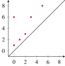
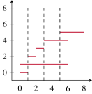
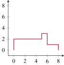
Given a persistence diagram $\mathcal{D}$, i.e., a descriptor of the topological activity of a data set Edelsbrunner10 , we can summarize topological features by calculating an associated persistence indicator function of $\mathcal{D}$ as

$$\mathds{1}_{\mathcal{D}}\colon \longrightarrow\mathds{N}$$ (1)

$$\epsilon \longmapsto\big{|}\big{\{}(c,d)\in\mathcal{D}\mid\epsilon\in[c,d]\big{\}}\big{|},$$

i.e., the number of points in the persistence diagram that, when being treated as a closed interval, contain the given parameter $\epsilon$. Equivalently, a PIF can be considered to describe the rank of the $p$^th homology group of a filtration of a simplicial complex. A PIF thus measures the amount of topological activity as a function of the threshold parameter $\epsilon$. This parameter is commonly treated as the “range” of a function defined on the given data set, e.g., a distance function Edelsbrunner02 or an elevation function Agarwal06 . Figure 1 demonstrates how to calculate the persistence indicator function $\mathds{1}_{\mathcal{D}}(\cdot)$ from a persistence diagram or, equivalently, from a persistence barcode. For the latter, the calculation becomes particularly easy. In the barcode, one only has to check the number of intervals that are intersected at any given time by a vertical line for some value of $\epsilon$.

3.1 Properties

We first observe that the PIF only changes at finitely many points. These are given by the creation and destruction times, i.e., the $x$- and $y$-coordinates, of points in the persistence diagram. The PIF may thus be written as a sum of appropriately scaled indicator functions (hence the name) of the form $\mathds{1}_{\mathcal{I}}(\cdot)$ for some interval $\mathcal{I}$. Within the interval $\mathcal{I}$, the value of $\mathds{1}_{\mathcal{D}}(\cdot)$ does not change. Hence, the PIF is a step function. Since step functions are compatible with addition and scalar multiplication, PIFs form a vector space. The addition of two PIFs corresponds to calculating the union of their corresponding persistence diagrams, while taking multiplicities of points into account. As a consequence, we can calculate the mean of a set of PIFs $\{\mathds{1}_{\mathcal{D}}^{1},\dots,\mathds{1}_{\mathcal{D}}^{n}\}$ as

$$\overline{\mathds{1}_{\mathcal{D}}}(\cdot):=\frac{1}{n}\sum_{i=1}^{n}\mathds{1}_{\mathcal{D}}^{i}(\cdot),$$ (2)

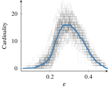
i.e., the standard pointwise mean of set of elements. In contrast to persistence diagrams, for which a mean is not uniquely defined and hard to calculate Turner14 , this calculation only involves addition (union) and scalar multiplications of sets of intervals. Figure 2 depicts mean persistence indicator functions for two randomly-sampled data sets. We see that the resulting mean persistence indicator functions already introduce a visual separation between the two data sets.

(a) Sphere ($r\approx 0.63$)

(b) Torus ($R=0.025$, $r=0.05$)

Figure 2: Mean persistence indicator function of the one-dimensional persistence diagrams of a sphere and of a torus. Both data sets have been sampled at random and are scaled such that their volume is the same.

As a second derived property, we note that the absolute value of a step function (and that of a PIF) always exists; one just calculates the absolute value for every interval in which the step function does not change. The absolute value of a step function is again a step function, so the Riemann integral of a PIF is well-defined, giving rise to their $1$-norm as

$$\|\mathds{1}_{\mathcal{D}}\|_{1}:=\int_{|}\mathds{1}_{\mathcal{D}}(x)|\operatorname{d}\!{x},$$ (3)

which is just the standard norm of an $\mathrm{L}^{\!1}$-space. The preceding equation requires the use of an absolute value because linear operations on PIFs may result in negative values. The integral of a PIF (or its absolute value) decomposes into a sum of integrals of individual step functions, defined over some interval $[a,b]$. Letting the value of the step function over this interval be $l$, the integral of the step function is given as $l\cdot|b-a|$, i.e., the volume of the interval scaled by the value the step function assumes on it. We can also extend this norm to that of an $\mathrm{L}^{\!p}$-space, where $p\in$. To do so, we observe that the $p$^th power of any step function is well-defined—we just raise the value it takes to the $p$^th power. Consequently, the $p$^th power of a PIF is also well-defined and we define

$$\|\mathds{1}_{\mathcal{D}}\|_{p}:=\Big{(}\int_{|}\mathds{1}_{\mathcal{D}}(x)|^{p}\operatorname{d}\!{x}\Big{)}^{\frac{1}{p}},$$ (4)

which is the standard norm of an $\mathrm{L}^{\!p}$-space. Calculating this integral again involves decomposing the range of the PIF into individual step functions and calculating their integral. We have $\|\mathds{1}_{\mathcal{D}}\|_{p}<\infty$ for every $p\in$ because there are only finitely many points in a persistence diagram, so the integrals of the individual step functions involved in the norm calculation are bounded.

Hypothesis Testing

Treating the norm of a PIF as a random variable, we can perform topology-based hypothesis testing similar to persistence landscapes Bubenik15 . Given two different samples of persistence diagrams, $\{\mathcal{D}^{1}_{1},\dots,\mathcal{D}^{1}_{n}\}$ and $\{\mathcal{D}^{2}_{1},\dots,\mathcal{D}^{2}_{n}\}$, we calculate the $1$-norm of their respective mean PIFs as $Y_{1}$ and $Y_{2}$, and the variances

$$\sigma_{i}^{2}:=\frac{1}{n-1}\sum_{j=1}^{n}\Big{(}\big{|}\mathds{1}_{\mathcal{D}^{i}_{j}}\big{|}-Y_{i}\Big{)}^{2},$$ (5)

for $i\in\{1,2\}$. We may then perform a standard two-sample $z$-test to check whether the two means are likely to be the same. To this end, we calculate the $z$-score as

$$z:=\frac{Y_{1}-Y_{2}}{\sqrt{s_{1}^{2}/n-s_{2}^{2}/n}}$$ (6)

and determine the critical values at the desired $\alpha$-level, i.e., the significance level, from the quantiles of a normal distribution. If $z$ is outside the interval spanned by the critical values, we reject the null hypothesis, i.e., we consider the two means to be different. For the example shown in Figure 2, we obtain $Y_{1}\approx 2.135$, $s_{1}^{2}\approx 0.074$, $Y_{2}\approx 2.79$, and $s_{2}^{2}\approx 0.093$. Using $\alpha=0.01$, the critical values are given by $z_{1}\approx-2.58$ and $z_{2}\approx 2.58$. Since $z\approx-11.09$, we reject the null hypothesis with $p\approx 1.44\times 10^{-28}\ll 0.01$. Hence, PIFs can be used to confidently discern random samples of a sphere from those of a torus with the same volume.

Stability The $1$-norm of a PIF is connected to the total persistence Cohen-Steiner10 , i.e., the sum of all persistence values in a persistence diagram. We have

$$\|\mathds{1}_{\mathcal{D}}\|_{1}=\int_{|}\mathds{1}_{\mathcal{D}}(x)|\operatorname{d}\!{x}=\sum_{I\in\mathcal{I}}c_{I}\operatorname{vol}(I),$$ (7)

where $\mathcal{I}$ denotes a set of intervals for which the number of active persistence pairs does not change, and $c_{I}$ denotes their count. We may calculate this partition from a persistence barcode, as shown in Figure 1b, by going over all the dotted slices, i.e., the intervals between pairs of start and endpoints of each interval. The sum over all these volumes is equal to the total persistence of the set of intervals, because we can split up the volume calculation of a single interval over many sub-interval and, in total, the volume of every interval is only accumulated once. Hence,

$$\|\mathds{1}_{\mathcal{D}}\|_{1}\int_{|}\mathds{1}_{\mathcal{D}}(x)|\operatorname{d}\!{x}=\sum_{(c,d)\in\mathcal{D}}|d-c|=\sum_{(c,d)\in\mathcal{D}}\operatorname{pers}(c,d)=\operatorname{pers}(\mathcal{D}),$$ (8)

where $\operatorname{pers}(\mathcal{D})$ denotes the total persistence of the persistence diagram. According to a stability theorem by Cohen-Steiner et al. Cohen-Steiner10 , the $1$-norm of a PIF is thus stable with respect to small perturbations. We leave the derivation of a similar equation for the general $\mathrm{L}^{\!p}$-norm of a PIF for future work.

3.2 The Bootstrap for Persistence Indicator Functions

Developed by Efron and Tibshirani Efron93 , the bootstrap is a general statistical method for—among other applications—computing confidence intervals. We give a quick and cursory introduction before showing how this method applies to persistence indicator functions; please refer to Chazal et al. Chazal13 for more details.

Assume that we have a set of independent and identically distributed variables $X_{1}$, …, $X_{n}$, and we want to estimate a real-valued parameter $\theta$ that corresponds to their distribution. Typically, we may estimate $\theta$ using a statistic $\widehat{\theta}:=s(X_{1},\dots,X_{n})$, i.e., some function of the data. A common example is to use $\theta$ as the population mean, while $\widehat{\theta}$ is the sample mean. If we want to calculate confidence intervals for our estimate $\widehat{\theta}$, we require the distribution of the difference $\theta-\widehat{\theta}$. This distribution, however, depends on the unknown distribution of the variables, so we have to approximate it using an empirical distribution. Let $X_{1}^{\ast}$, …, $X_{n}^{\ast}$ be a sample of the original variables, drawn with replacement. We can calculate $\widehat{\theta}^{\ast}:=s(X_{1}^{\ast},\dots,X_{n}^{\ast})$ and approximate the unknown distribution by the empirical distribution of $\widehat{\theta}-\widehat{\theta}^{\ast}$, which, even though it is not computable analytically, can be approximated by repeating the sampling procedure a sufficient number of times. The quantiles of the approximated distribution may then be used to construct confidence intervals, leading to the following method:

1. Calculate an estimate of $\theta$ from the input data using $\widehat{\theta}:=s(X_{1},\dots,X_{n})$.

2. Obtain $X_{1}^{\ast}$, …, $X_{n}^{\ast}$ (sample with replacement) and calculate $\widehat{\theta}^{\ast}:=s(X_{1}^{\ast},\dots,X_{n}^{\ast})$.

3. Repeat the previous step $B$ times to obtain $\widehat{\theta}^{\ast}_{1}$, …, $\widehat{\theta}^{\ast}_{B}$.

4. Given $\alpha$, compute an approximate $(1-2\alpha)$ quantile interval as

   $$[\widehat{\theta}_{1},\widehat{\theta}_{2}]\approx[\widehat{\theta}^{\ast(\alpha)}_{B},\widehat{\theta}^{\ast(1-\alpha)}_{B}],$$ (9)

   where $\widehat{\theta}^{\ast(\alpha)}_{B}$ refers to the $\alpha$^th empirical quantile of the bootstrap replicates from the previous step.

This procedure yields both a lower bound and an upper bound for $\widehat{\theta}$. It is also referred to as the percentile interval for bootstraps (Efron93, , pp. 168–176). More complicated versions—yielding “tighter” confidence intervals—of this procedure exist, but the basic method of sampling with replacement and computing the statistic $s(\cdot)$ on the bootstrap samples remains the same.

(a) Sphere

(b) Torus

Figure 3: Confidence bands at the $\alpha=0.05$ level for the mean persistence indicator functions of a sphere and a torus. The confidence band is somewhat tighter for $\epsilon\geq 0.2$.

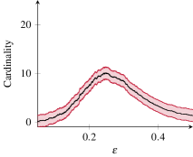
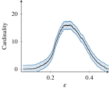
In order to apply the bootstrap to functions, we require empirical processes Kosorok08 . The goal is to find a confidence band for a function $f(x)$, i.e., a pair of functions $l(x)$ and $u(x)$ such that the probability that $f(x)\in[l(x),u(x)]$ for $x\in$ is at least $1-\alpha$. Given a function $f$, let $Pf:=\int f\operatorname{d}\!{P}$ and $P_{n}f:=n^{-1}\sum_{i=1}^{n}f(X_{i})$. We obtain a bootstrap empirical process as

$$\{\mathds{P}f\}_{f\in\mathcal{F}}:=\{\sqrt{n}\left(P_{n}^{\ast}f-P_{n}f\right)\},$$ (10)

where $P_{n}^{\ast}:=n^{-1}\sum_{i=1}^{n}f(X_{i}^{\ast})$ is defined on the bootstrap samples (as introduced above). Given the convergence of this empirical process, we may calculate

$$\widehat{\theta}:=\sup_{f\in\mathcal{F}}|\mathds{P}f|,$$ (11)

which yields a statistic to use for the bootstrap as defined above. From the corresponding quantile, we ultimately obtain $[\widehat{\theta}_{1},\widehat{\theta}_{2}]$ and calculate a confidence band

$$C_{n}(f):=\left[P_{n}f-\frac{\widehat{\theta}_{1}}{n},P_{n}f+\frac{\widehat{\theta}_{2}}{n}\right]$$ (12)

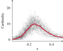
for the empirical mean of a set of PIFs. Figure 3 depicts an example of confidence bands for the mean PIF of the sphere and torus samples. We can see that the confidence band for the torus is extremely tight for $\epsilon\in[0.2,0.3]$, indicating that the limit behavior of samples from a torus is different at this scale from the limit behavior of samples from a sphere.

3.3 Distances and Kernels

Given two persistence diagrams $\mathcal{D}_{i}$ and $\mathcal{D}_{j}$, we are often interested in their dissimilarity (or distance). Having seen that linear combinations and norms of PIFs are well-defined, we can define a family of distances as

$$\operatorname{dist}_{p}(\mathds{1}_{\mathcal{D}_{i}},\mathds{1}_{\mathcal{D}_{j}}):=\Big{(}\int_{|}\mathds{1}_{\mathcal{D}_{i}}(x)-\mathds{1}_{\mathcal{D}_{j}}(x)|^{p}\operatorname{d}\!{x}\Big{)}^{\frac{1}{p}},$$ (13)

with $p\in$. Since the norm of a PIF is well-defined, this expression is a metric in the mathematical sense. Note that its calculation requires essentially only evaluating all individual step functions of the difference of the two PIFs once. Hence, its complexity is linear in the number of sub-intervals.

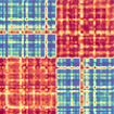
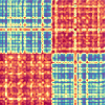
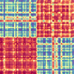
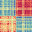
Example Figure 4 depicts pairwise distance matrices for random samples of a sphere and of a torus. The first matrix of each group is obtained via $\operatorname{dist}_{p}$ for PIFs, while the second matrix in each group is obtained by the $p$^th Wasserstein distance. We observe two groups of data sets in all matrices, meaning that both classes of distances are suitable for detecting differences.

(a) $p=1$

(b) $p=2$

Figure 4: A comparison of distance matrices obtained using the distance measure $\operatorname{dist}_{p}$ for PIFs, and the corresponding $p$^th Wasserstein distance $\operatorname{W\!}_{p}$. The left matrix of each group shows $\operatorname{dist}_{p}$, while the right matrix depicts $\operatorname{W\!}_{p}$. Red indicates close objects (small distances), while blue indicates far objects (large distances).

We can also employ the distance defined above to obtain a kernel Schoelkopf02 . To this end, we define

$$k_{p}(\mathcal{D}_{i},\mathcal{D}_{j}):=-\operatorname{dist}_{p}(\mathds{1}_{\mathcal{D}_{i}},\mathds{1}_{\mathcal{D}_{j}}),$$ (14)

where $p\in\{1,2\}$ because we need to make sure that the kernel is conditionally positive definite Schoelkopf02 . This kernel permits using PIFs with many modern machine learning algorithms. As an illustrative example, we will use kernel support vector machines Schoelkopf02 to separate random samples of a sphere and a torus.

Example Again, we use 100 random samples (50 per class) from a sphere and a torus. We only use one-dimensional persistence diagrams, from which we calculate PIFs, from which we then obtain pairwise kernel matrices using both $k_{1}$ and $k_{2}$. Finally, we train a support vector machine using nested stratified $5$-fold cross-validation. With $k_{1}$, we obtain an average accuracy of $0.98\pm 0.049$, whereas with $k_{2}$, we obtain an average accuracy of $0.95\pm 0.063$. The decrease in accuracy is caused by the additional smoothing introduced in this kernel.

4 Applications

In the following, we briefly discuss some potential application scenarios for PIFs. We use only data sets that are openly available in order to make our results comparable. For all machine learning methods, we use scikit-learn Pedregosa11 .

4.1 Analysis of Random Complexes

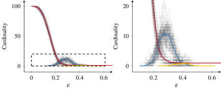
It is often useful to know to what extent a data set exhibits random fluctuations. To this end, we sampled 100 points from a unit cube in ³, which has the topology of a point, i.e., no essential topological features in dimensions $>0$. We calculated the Vietoris–Rips complex at a scale such that no essential topological features remain in dimensions $\geq 1$, and obtained PIFs, which are depicted in Figure 5 along with their corresponding mean. All functions use a common axis in order to simplify their comparison. We first comment on the dynamics of these data. Topological activity is “shifted”, meaning that topological features with a different dimensionality are not active at the same scale. The maximum of topological activity in dimension one (blue curve) is only reached when there are few zero-dimensional features. The maximum in dimension two (yellow curve) also does not coincide with the maximum in dimension one. These results are consistent with a limit theorem of Bobrowski and Kahle Bobrowski14 , who showed that (persistent) Betti numbers follow a Poisson distribution.

Figure 5: PIFs for random complexes sampled over a unit cube in ³. Dimensions zero (red), one (blue), and two (yellow) are shown. To show the peak in dimension two better, the right-hand side shows a “zoomed” version of the first chart (dashed region).

Figure 6: PIFs for random samples of a sphere with $r=1.0$. Again, dimensions zero (red), one (blue), and two (yellow) are shown, along with a “zoomed” version of the first chart (dashed region).

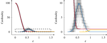
By contrast, for a data set with a well-defined topological structure, such as a $2$-sphere, the PIFs exhibit a different behavior. Figure 6 depicts all PIFs of random samples from a sphere. We did not calculate the Vietoris–Rips complex for all possible values of $\epsilon$ but rather selected an $\epsilon$ that is sufficiently large to capture the correct Betti numbers of the sphere. Here, we observe that the stabilization of topological activity in dimension zero roughly coincides with the maximum of topological activity in dimension one. Topological activity in dimension two only starts to increase for larger scales, staying stable for a long interval. This activity corresponds to the two-dimensional void of the $2$-sphere that we detect using persistent homology.

PIFs can thus be used to perform a test for “topological randomness” in real-world data. This is useful for deciding whether a topological approximation is suitable or needs to be changed (e.g., by calculating a different triangulation, using $\alpha$-shapes, etc.). Moreover, we can use a PIF to detect the presence or absence of a shared “scale” in data sets. For the random complexes, there is no value for $\epsilon$ in which stable topological activity occurs in more than one dimension, whereas for the sphere, we observe a stabilization starting from $\epsilon\approx 0.75$.

4.2 Shakespearean Co-Occurrence Networks

In a previous work, co-occurrence networks from a machine-readable corpus of Shakespeare’s plays Rieck16b have been extracted. Their topological structure under various aspects has been analyzed, using, for example, their clique communities Rieck17 to calculate two-dimensional embeddings of the individual networks. The authors observed that comedies form clusters in these embeddings, which indicates that they are more similar to each other than to plays of another category. Here, we want to show that it is possible to differentiate between comedies and non-comedies by using the kernel induced by PIFs. Among the 37 available plays, 17 are comedies, giving us a baseline probability of $0.46$ if we merely “guess” the class label of a play. Since the number of plays is not sufficiently large to warrant a split into test and training data, we use various cross-validation techniques, such as leave-one-out. The reader is referred to Kohavi Kohavi95 for more details. Table 1 reports all results; we observe that $k_{1}$ outperforms $k_{2}$. Since $k_{2}$ emphasizes small-scale differences, the number of topological features in two networks that are to be compared should be roughly equal. This is not the case for most of the comedies, though. We stress that these results are only a demonstration of the capabilities of PIFs; the comparatively low accuracy is partially due to the fact that networks were extracted automatically. It is interesting to note which plays tend to be mislabeled. For $k_{1}$, All’s Well That Ends Well, Cymbeline, and The Winter’s Tale are mislabeled more than all other plays. This is consistent with research by Shakespeare scholars who suggest different categorization schemes for these (and other) problem plays.

Table 1: Classifier performance for Shakespearean co-occurrence networks. Classification based on $k_{1}$ outperforms the second kernel $k_{2}$.

Kernel	$5$-fold	LOO	LPO ($p=2$)	LPO ($p=3$)	LPO ($p=4$)	Split
$k_{1}$	0.84	0.83	0.83	0.80	0.79	0.80
$k_{2}$	0.64	0.00	0.67	0.68	0.68	0.68

4.3 Social Networks

Yanardag and Vishwanathan Yanardag15 crawled the popular social news aggregation website reddit.com in order to obtain a set of graphs from online discussions. In each graph, the nodes correspond to users and an edge signifies that a certain user responded to a another user’s comment. The graphs are partitioned into two classes, one of them representing discussion-based forums (in which users typically communicate freely among each other), the other representing communities based on a question–answer format (in which users typically only respond to the creator of a topic). The data set is fully-balanced.

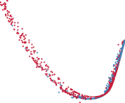
Here, we want to find out whether it is possible to classify the graphs using nothing but topological information. We use the degree, i.e., the number of neighbors, of a node in the graph to obtain a filtration, assigning every edge the maximum of the degrees of its endpoints. We then calculate one-dimensional persistent homology and our kernel for $p=1$ and $p=2$. Figure 7 shows the results of applying kernel principal component analysis (k-PCA) Schoelkopf98 , which each point in the embedding corresponding to a single graph. A small set of outliers appears to “skew” the embedding (Figure 7a), but an inspection of the data shows that these graphs are extremely small (and sparse) in contrast to the remaining graphs. After removing them, the separation between both classes is visibly better (Figure 7b). Progress from “left” to “right” in the embedding, graphs tend to become more dense.

(a) Original data

(b) Cleaned data

Figure 7: Embeddings based on k-PCA for the $k_{1}$ kernel. LABEL:sub@sfig:reddit_PCA_original Every node represents a certain graph. The color indicates a graph from a discussion-based forum (red) or a Q/A forum (blue). LABEL:sub@sfig:reddit_PCA_cleaned We removed some outliers to obtain a cleaner output. It is readily visible that the two classes suffer from overlaps, which influence classification performance negatively.

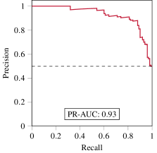
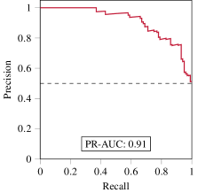
As a second application on these data, we use a kernel support vector machine to classify all graphs, without performing outlier removal. We split the data into training (90%) and test (10%) data, and use $4$-fold cross validation to find the best hyperparameters. The average accuracy for $k_{1}$ is $0.88$, while the average accuracy for $k_{2}$ is $0.81$. PIFs thus manage to surpass previous results by Yanardag and Vishwanathan Yanardag15 , which employed a computationally more expensive strategy, i.e., graph kernels Sugiyama17 based on learned latent sub-structures, and obtained an average accuracy of $0.78$ for these data. Figure 8 depicts precision–recall curves for the two kernels. The kernel $k_{1}$ manages to retain higher precision at higher values of recall than $k_{2}$, which is again due to its lack of smoothing.

(a) $k_{1}$

(b) $k_{2}$

Figure 8: Precision–recall curves for both kernels on the social networks data set. Each curve also includes the area-under-the-curve (AUC) value.

5 Conclusion

This paper introduced persistence indicator functions (PIFs), a novel class of summarizing functions for persistence diagrams. While being approximative by nature, we demonstrated that they exhibit beneficial properties for data analysis, such as the possibility to perform bootstrap experiments, calculate distances, and use kernel-based machine learning methods. We tested the performance on various data sets and illustrated the potential of PIFs for topological data analysis and topological machine learning. In the future, we want to perform a more in-depth analysis of the mathematical structure of PIFs, including detailed stability theorems, approximation guarantees, and a description of their statistical properties.

References

- (1) Adams, H., Emerson, T., Kirby, M., Neville, R., Peterson, C., Shipman, P., Chepushtanova, S., Hanson, E., Motta, F., Ziegelmeier, L.: Persistence images: A stable vector representation of persistent homology. Journal of Machine Learning Research 18(8), 1–35 (2017)
- (2) Agarwal, P.K., Edelsbrunner, H., Harer, J., Wang, Y.: Extreme elevation on a 2-manifold. Discrete & Computational Geometry 36(4), 553–572 (2006)
- (3) Bobrowski, O., Kahle, M.: Topology of random geometric complexes: a survey (2014). URL https://arxiv.org/abs/1409.4734
- (4) Bremer, P.T., Edelsbrunner, H., Hamann, B., Pascucci, V.: A topological hierarchy for functions on triangulated surfaces. IEEE Transactions on Visualization and Computer Graphics 10(4), 385–396 (2004). DOI 10.1109/TVCG.2004.3
- (5) Bubenik, P.: Statistical topological data analysis using persistence landscapes. Journal of Machine Learning Research 16, 77–102 (2015)
- (6) Chazal, F., Fasy, B.T., Lecci, F., Rinaldo, A., Singh, A., Wasserman, L.: On the bootstrap for persistence diagrams and landscapes. Modeling and Analysis of Information Systems 20(6), 111–120 (2013)
- (7) Cohen-Steiner, D., Edelsbrunner, H., Harer, J.: Stability of persistence diagrams. Discrete & Computational Geometry 37(1), 103–120 (2007)
- (8) Cohen-Steiner, D., Edelsbrunner, H., Harer, J., Mileyko, Y.: Lipschitz functions have -stable persistence. Foundations of Computational Mathematics 10(2), 127–139 (2010)
- (9) Edelsbrunner, H., Harer, J.: Computational topology: An introduction. AMS (2010)
- (10) Edelsbrunner, H., Letscher, D., Zomorodian, A.J.: Topological persistence and simplification. Discrete & Computational Geometry 28(4), 511–533 (2002)
- (11) Edelsbrunner, H., Morozov, D.: Persistent homology: Theory and practice. In: European Congress of Mathematics. EMS Publishing House, Zürich, Switzerland (2014)
- (12) Efron, B., Tibshirani, R.J.: An introduction to the bootstrap. No. 57 in Monographs on Statistics and Applied Probability. Chapman & Hall/CRC, Boca Raton, FL, USA (1993)
- (13) Günther, D., Boto, R.A., Contreras-Garcia, J., Piquemal, J.P., Tierny, J.: Characterizing molecular interactions in chemical systems. IEEE Transactions on Visualization and Computer Graphics 20(12), 2476–2485 (2014)
- (14) Kerber, M., Morozov, D., Nigmetov, A.: Geometry helps to compare persistence diagrams. In: M. Goodrich, M. Mitzenmacher (eds.) Proceedings of the 18th Workshop on Algorithm Engineering and Experiments (ALENEX), pp. 103–112. SIAM, Philadelphia, PA, USA (2016)
- (15) Kohavi, R.: A study of cross-validation and bootstrap for accuracy estimation and model selection. In: Proc. IJCAI, vol. 2, pp. 1137–1143 (1995)
- (16) Kosorok, M.R.: Introduction to Empirical Processes and Semiparametric Inference. Springer, New York, NY, USA (2008)
- (17) Laney, D., Bremer, P.T., Mascarenhas, A., Miller, P., Pascucci, V.: Understanding the structure of the turbulent mixing layer in hydrodynamic instabilities. IEEE Transactions on Visualization and Computer Graphics 12(5), 1053–1060 (2006)
- (18) Mucha, M., Sankowski, P.: Maximum matchings via Gaussian elimination. In: 45th Annual IEEE Symposium on Foundations of Computer Science, pp. 248–255 (2004)
- (19) Pedregosa, F., Varoquaux, G., Gramfort, A., Michel, V., Thirion, B., Grisel, O., Blondel, M., Prettenhofer, P., Weiss, R., Dubourg, V., Vanderplas, J., Passos, A., Cournapeau, D., Brucher, M., Perrot, M., Duchesnay, É.: Scikit-learn: Machine learning in Python. Journal of Machine Learning Research 12, 2825–2830 (2011)
- (20) Reininghaus, J., Huber, S., Bauer, U., Kwitt, R.: A stable multi-scale kernel for topological machine learning. In: IEEE Conference on Computer Vision and Pattern Recognition (CVPR), pp. 4741–4748. Curran Associates, Inc., Red Hook, NY, USA (2015)
- (21) Rieck, B., Fugacci, U., Lukasczyk, J., Leitte, H.: Clique community persistence: A topological visual analysis approach for complex networks. IEEE Transactions on Visualization and Computer Graphics (2017). To appear.
- (22) Rieck, B., Leitte, H.: Shall I compare thee to a network?—Visualizing the topological structure of Shakespeare’s plays. In: Workshop on Visualization for the Digital Humanities at IEEE VIS. Baltimore, MD (2016)
- (23) Schölkopf, B., Smola, A.J.: Learning with Kernels. The MIT Press, Cambridge, MA, USA (2002)
- (24) Schölkopf, B., Smola, A.J., Müller, K.R.: Nonlinear component analysis as a kernel eigenvalue problem. Neural Computation 10(5), 1299–1319 (1998)
- (25) Sugiyama, M., Ghisu, M.E., Llinares-López, F., Borgwardt, K.: graphkernels: R and Python packages for graph comparison. Bioinformatics 34(3), 530–532 (2017)
- (26) Turner, K., Mileyko, Y., Mukherjee, S., Harer, J.: Fréchet means for distributions of persistence diagrams. Discrete & Computational Geometry 52(1), 44–70 (2014)
- (27) Yanardag, P., Vishwanathan, S.V.N.: Deep graph kernels. In: Proceedings of the 21th ACM SIGKDD International Conference on Knowledge Discovery and Data Mining, pp. 1365–1374. ACM, New York, NY, USA (2015)