Hierarchies and Ranks for Persistence Pairs

Abstract

We develop a novel hierarchy for zero-dimensional persistence pairs, i.e., connected components, which is capable of capturing more fine-grained spatial relations between persistence pairs. Our work is motivated by a lack of spatial relationships between features in persistence diagrams, leading to a limited expressive power. We build upon a recently-introduced hierarchy of pairs in persistence diagrams that augments the pairing stored in persistence diagrams with information about which components merge. Our proposed hierarchy captures differences in branching structure. Moreover, we show how to use our hierarchy to measure the spatial stability of a pairing and we define a rank function for persistence pairs and demonstrate different applications.

1 Introduction

A wide range of application domains employ the concept of persistence, i.e., a measure of feature robustness or scale. It is particularly effective when dealing with noisy data, permitting analysts to distinguish between “signal” and “noise”. Being a purely topological approach, however, the information conferred by persistence does not retain any spatial information. While this is sometimes desirable, previous work Gerber10 ; Rieck14b ; Zomorodian08 has shown that retaining at least a minimum of geometrical information is often beneficial, as it increases the expressive power. In this paper, we develop a hierarchy that relates points in a persistence diagram. Our hierarchy makes exclusive use of topological properties of data, while still being able to distinguish between geometrically distinct data. Moreover, the hierarchy is capable of measuring stability properties of the pairing of critical points itself, yielding additional structural stability information about input data. We demonstrate the practicality of our method by means of several datasets. Additionally, we compare it to a state-of-the-art hierarchy, point out the improvements over said hierarchy, and demonstrate how our novel approach differs from related hierarchical concepts such as Reeb graphs.

2 Related Work

We refer the reader to Edelsbrunner and Harer Edelsbrunner10 for a detailed overview of persistence and related concepts. There are several related approaches for creating a hierarchy of persistence information. Doraiswamy et al. Doraiswamy13 calculate a topological saliency of critical points in a scalar field based on their spatial arrangement. Critical points with low persistence that are isolated from other critical points have a higher saliency in this concept. These calculations yield saliency curves for different smoothing radii. While these curves permit a ranking of persistence pairs, they do not afford a description of their nesting behavior. Consequently, in contrast to our approach, the saliency approach is incapable of distinguishing some spatial rearrangements that leave persistence values and relative distances largely intact, such as moving all peaks towards each other. Bauer Bauer11 developed what we refer to in this paper as the regular persistence hierarchy. It is fully combinatorial and merely requires small changes of the pairing calculation of related critical points. This hierarchy was successfully used in determining cancellation sequences of critical points of surfaces. However, as shown in this paper, this hierarchy cannot distinguish between certain nesting relations.

In scalar field analysis, the calculation of graph structures such as the Reeb graph Doraiswamy09 or the contour tree Carr03 , along with merge and split trees, has a long tradition. These graphs relate critical points with each other, but do not permit the calculation of hierarchies of persistence pairs. We will demonstrate this on a simple one-dimensional example in this paper. Recent work in this area is driven by the same motivation as our work: the merge tree, for example, turns out to be more expressive with respect to spatial differences in the domain. Thus, even if two scalar fields have the same critical pairs, their merge trees are capable of retaining differences in sublevel set merging behavior. This observation led to the development of distance measures for merge trees Beketayev14 , Reeb graphs Bauer14 , and extremum graphs Narayanan15 . Since the aforementioned tree structures tend to be unwieldy, Pascucci et al. Pascucci09 proposed a hierarchical decomposition, the branch decomposition. This decomposition relates the different branches of a contour tree with each other. Recently, Saikia et al. Saikia14 used these graphs as a similarity measure for the structural comparison of scalar data. While these works are close to our method in spirit, they rely on a different type of structural information.

3 Background and Notation

In this paper, we assume that we are working with a domain $\mathds{D}$ and a scalar function $f\colon\mathds{D}\to$. We make no assumptions about the connectivity of $\mathds{D}$ or its dimension. As for $f$, we require it to have a finite number of critical points—a condition that is always satisfied for real-world data—and that the function values of those critical points are different—a condition that may be satisfied by, e.g., symbolic perturbation Edelsbrunner90 . Such scalar fields commonly occur in many different applications, and their features are often described using scalar field topology. This umbrella term refers to the analysis of how certain special sets—the level sets—of the scalar function $f$ change upon varying parameters. More precisely, given a threshold $c$, one typically distinguishes between, e.g., level set $\mathcal{L}_{c}(f)$, and sublevel set $\mathcal{L}_{c}^{-}(f)$,

$$\mathcal{L}_{c}(f):= \left\{x\in\mathds{D}\mid f\left(x\right)=c\right\}$$ (1)

$$\mathcal{L}_{c}^{-}(f):= \left\{x\in\mathds{D}\mid f\left(x\right)\leq c\right\}$$ (2)

In this paper, we also require the interlevel set $\mathcal{L}_{l,u}(f)$,

$$\mathcal{L}_{l,u}(f):=\mathcal{L}_{u}^{-}(f)\setminus\mathcal{L}_{l}^{-}(f)=\{x\in\mathds{D}\mid l\leq f(x)\leq u\}.$$ (3)

Interlevel sets are commonly used to describe the topology of real-valued functions Carlsson09a or the robustness of homology classes Bendich10 ; Bendich13 . Scalar field topology refers to the investigation of changes in connectivity in these sets. Such changes are intricately connected to the critical points of $f$ by means of Morse theory Milnor63 . Focusing on the sublevel sets (the case for superlevel sets can be solved by duality arguments), we find that (local) minima create new connected components in the sublevel set, while (local) maxima—or saddles in higher dimensions—are responsible for merging two connected components, thereby destroying one of them. Related creators and destroyers may thus be paired with each other (using, e.g., the “elder rule” (Edelsbrunner10, , p. 150) that merges the connected component with a higher—younger—function value into the one with a lower—older—function value), which permits their use in various data structures.

The persistence diagram is a generic data structure to represent such a pairing. For every creator–destroyer pair, it contains a point in ² according to the corresponding function values. Persistence diagrams have many desirable stability properties Cohen-Steiner07 ; Cohen-Steiner10 and permit the calculation of different metrics. Unfortunately, they are sometimes too coarse to describe both the topology and geometry of a scalar function. Given a point $(c,d)$ in a persistence diagram, where $c$ is the function value of the creator and $d$ is the function value of the paired destroyer, the absolute difference $|d-c|$ is referred to as the persistence $\operatorname{pers}(c,d)$ of the pair. Persistence permits a way to define whether certain pairs are more prominent than others. Roughly speaking, the persistence of such a pair is the magnitude of the smallest perturbation that is able to cancel it.

4 Persistence Hierarchies

The calculation of persistence always underlies the idea of a pairing, i.e., a way of relating different parts of a function with each other. Here, we shall only focus on zero-dimensional persistent homology, which describes connected components in the sublevel sets of a function, and the elder rule for pairing points. Consequently, we have a relationship between local minima and local maxima (or saddles in higher dimensions) of a function. We leave the treatment of other topological features for future work. Moreover, we only cover the case of sublevel sets; superlevel set calculations follow by analogy.

4.1 Regular Persistence Hierarchy

Bauer Bauer11 observes that the process of merging two connected components permits the definition of a natural hierarchy between persistence pairs. More precisely, assume that we are given two connected components $\sigma$ and $\sigma^{\prime}$, each created at a local minimum. If $\sigma$ merges into $\sigma^{\prime}$ at, e.g., a local maximum, we consider $\sigma^{\prime}$ to be the parent of $\sigma$. This relation is a necessary but not sufficient condition for finding out which pairs of critical points of a Morse function cannot be canceled without affecting other points. We call this hierarchy, which is equivalent to a merge tree Carr03 , the regular persistence hierarchy. Each of its nodes corresponds to a creator–destroyer pair. The hierarchy forms a directed acyclic graph, i.e., a tree. This is a consequence of the assumption that the function values at critical points are unique. Thus, whenever a merge of two connected components takes place, the “younger” component is uniquely defined. Moreover, a critical point cannot both create and destroy a topological feature, so there cannot be any cycles in the hierarchy. The regular persistence hierarchy has a natural root that corresponds to the global minimum, as the connected component corresponding to this value is never merged.

Example and limitations The regular persistence hierarchy cannot distinguish some connectivity relations: for example, Fig. 1 depicts the regular persistence hierarchies for two simple functions. We can see that the hierarchy is equal for both functions even though their connectivity behavior is different. More precisely, in the red function, the two persistence pairs are connected via two different branches of the function, i.e., it is impossible to reach both minima without traversing a third minimum—the global one—as the threshold of the sublevel sets is increased. This difference in connectivity results in a different stability of the pairing. A perturbation of the critical points at and in the blue function, for example, is capable of changing the complete pairing: if we move the points to $f(4)=1.9$ and $f(5)=0.9$, respectively, the pairing of the critical point at $x=1$ will change, as well. The same perturbation has no effect on the red function, though. A hierarchy of persistence pairs should account for these differences in connectivity.

(a) Functions

(b) Persistence diagram

(c) Hierarchy

Figure 1: Two functions with different connectivity but equal persistence diagrams. Both functions also share the same regular persistence hierarchy.

4.2 Interlevel Set Persistence Hierarchy (ISPH)

The example depicted in Fig. 1 demonstrated a lack of discriminating information in the regular persistence hierarchy. The key observation, illustrated as running example in Fig. 2, is that not every merge of two connected components is topologically equal: a merge may either result in a different branching structure of the hierarchy or it may keep the branches intact. Fig. 3 depicts our proposed interlevel set persistence hierarchy (ISPH). To measure these differences, we propose extending the traditional union–find data structure that is used to detect the merges. Instead of merely storing the parent node of a given connected component in the hierarchy, i.e., the generating critical point with lowest function value, we also store $\hat{c}$, the highest minimum—in terms of the function value—along this branch. This will permit us to decide whether an additional branch needs to be introduced, as is the case for function 2(a) in Fig. 2. If $\hat{c}$ of a connected component is identical to the value of the parent, we call this assignment trivial. We will use $\hat{c}$ interchangeably both for the critical point as well as for its function value. Subsequently, we distinguish between two types of merges: the first type of merge only extends a branch in the hierarchy, while the second type of merge results in two branches that need to be unified at a third critical point. Fig. 2 depicts the two cases for the example functions shown in Fig. 1. We can see that for function 2(a), the pairs of critical points are connected by an additional critical point  only. Hence, two branches of the hierarchy merge at this point. Function 2(b), by contrast, merely prolongs a branch in the hierarchy—both pairs of critical points of the function are already connected without the inclusion of an additional critical point.

(a)

(b)

Figure 2: The merge phase of the interlevel set persistence hierarchy (ISPH)makes use of the connectivity of the interlevel set (hatched lines): to connect the critical point pairs $(b,y)$ and $(c,z)$ in 2(a), a region belonging to a third critical point  needs to be traversed. This is not the case for 2(b).

Figure 3: The ISPHs for the example functions shown in Fig. 1. In contrast to the regular persistence hierarchy, our hierarchy is capable of discriminating between the two functions. The hierarchy on the right has been rotated for layout reasons.

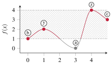
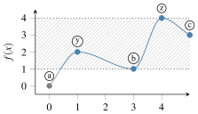
To distinguish between these two cases, we check the stored highest critical points $\hat{c}_{l}$ and $\hat{c}_{r}$ of the two connected components that merge at a local extremum. Without loss of generality, we assume that $\hat{c}_{l}$ belongs to the “older” branch and $\hat{c}_{r}$ belongs to the “younger” branch. If both $\hat{c}_{l}$ and $\hat{c}_{r}$ are trivial, we merge their respective branches just as for the regular persistence hierarchy. Else, we have to check the induced connectivity to decide how the branches should be connected. To this end, let $y_{u}$ refer to the value of the current critical point, i.e., the one at which the two connected components merge. Furthermore, let $y_{l}$ refer to $\min(\hat{c}_{l},\hat{c}_{r})$, the oldest of the two stored critical points. We now calculate the interlevel set $\mathcal{L}_{y_{l},y_{u}}(f)$; see the colored parts in Fig. 2 for an example. Following this, we check whether $\hat{c}_{l}$ and $\hat{c}_{r}$ are in the same connected component with respect to $\mathcal{L}_{y_{l},y_{u}}(f)$. If so, the current branch can be prolonged and $\hat{c}_{l}$ is set to $\hat{c}_{r}$. If not, two branches meet at the current critical point and merge into one. In Fig. 2(a), upon reaching , we merge components and , giving rise to the pair $(b,y)$. We have trivial critical points, i.e., $\hat{c}_{l}={\scriptsize\leavevmode\hbox to7.85pt{\vbox to7.85pt{\pgfpicture\makeatletter\hbox{\hskip 3.92485pt\lower-3.92485pt\hbox to0.0pt{\pgfsys@beginscope\pgfsys@invoke{ }\definecolor{pgfstrokecolor}{rgb}{0,0,0}\pgfsys@color@rgb@stroke{0}{0}{0}\pgfsys@invoke{ }\pgfsys@color@rgb@fill{0}{0}{0}\pgfsys@invoke{ }\pgfsys@setlinewidth{0.4pt}\pgfsys@invoke{ }\nullfont\hbox to0.0pt{\pgfsys@beginscope\pgfsys@invoke{ }{ {{}}\hbox{\hbox{{\pgfsys@beginscope\pgfsys@invoke{ }\definecolor[named]{pgffillcolor}{rgb}{1,1,1}\pgfsys@color@gray@fill{1}\pgfsys@invoke{ }{{}{{{}}}{{}}{}{}{}{}{}{}{}{}{}{\pgfsys@beginscope\pgfsys@invoke{ }\definecolor[named]{pgffillcolor}{rgb}{1,1,1}\pgfsys@color@gray@fill{1}\pgfsys@invoke{ }{}\pgfsys@moveto{3.72485pt}{0.0pt}\pgfsys@curveto{3.72485pt}{2.0572pt}{2.0572pt}{3.72485pt}{0.0pt}{3.72485pt}\pgfsys@curveto{-2.0572pt}{3.72485pt}{-3.72485pt}{2.0572pt}{-3.72485pt}{0.0pt}\pgfsys@curveto{-3.72485pt}{-2.0572pt}{-2.0572pt}{-3.72485pt}{0.0pt}{-3.72485pt}\pgfsys@curveto{2.0572pt}{-3.72485pt}{3.72485pt}{-2.0572pt}{3.72485pt}{0.0pt}\pgfsys@closepath\pgfsys@moveto{0.0pt}{0.0pt}\pgfsys@fillstroke\pgfsys@invoke{ } \pgfsys@invoke{\lxSVG@closescope }\pgfsys@endscope}{{{{}}\pgfsys@beginscope\pgfsys@invoke{ }\pgfsys@transformcm{1.0}{0.0}{0.0}{1.0}{-1.75pt}{-1.50694pt}\pgfsys@invoke{ }\hbox{{\definecolor{pgfstrokecolor}{rgb}{0,0,0}\pgfsys@color@rgb@stroke{0}{0}{0}\pgfsys@invoke{ }\pgfsys@color@rgb@fill{0}{0}{0}\pgfsys@invoke{ }\hbox{{a}} }}\pgfsys@invoke{\lxSVG@closescope }\pgfsys@endscope}}} \pgfsys@invoke{\lxSVG@closescope }\pgfsys@endscope}}} } \pgfsys@invoke{\lxSVG@closescope }\pgfsys@endscope{{{}}}{}{}\hss}\pgfsys@discardpath\pgfsys@invoke{\lxSVG@closescope }\pgfsys@endscope\hss}}\lxSVG@closescope\endpgfpicture}}}$ and $\hat{c}_{r}={\scriptsize\leavevmode\hbox to9.41pt{\vbox to9.41pt{\pgfpicture\makeatletter\hbox{\hskip 4.70366pt\lower-4.70366pt\hbox to0.0pt{\pgfsys@beginscope\pgfsys@invoke{ }\definecolor{pgfstrokecolor}{rgb}{0,0,0}\pgfsys@color@rgb@stroke{0}{0}{0}\pgfsys@invoke{ }\pgfsys@color@rgb@fill{0}{0}{0}\pgfsys@invoke{ }\pgfsys@setlinewidth{0.4pt}\pgfsys@invoke{ }\nullfont\hbox to0.0pt{\pgfsys@beginscope\pgfsys@invoke{ }{ {{}}\hbox{\hbox{{\pgfsys@beginscope\pgfsys@invoke{ }\definecolor[named]{pgffillcolor}{rgb}{1,1,1}\pgfsys@color@gray@fill{1}\pgfsys@invoke{ }{{}{{{}}}{{}}{}{}{}{}{}{}{}{}{}{\pgfsys@beginscope\pgfsys@invoke{ }\definecolor[named]{pgffillcolor}{rgb}{1,1,1}\pgfsys@color@gray@fill{1}\pgfsys@invoke{ }{}\pgfsys@moveto{4.50366pt}{0.0pt}\pgfsys@curveto{4.50366pt}{2.48734pt}{2.48734pt}{4.50366pt}{0.0pt}{4.50366pt}\pgfsys@curveto{-2.48734pt}{4.50366pt}{-4.50366pt}{2.48734pt}{-4.50366pt}{0.0pt}\pgfsys@curveto{-4.50366pt}{-2.48734pt}{-2.48734pt}{-4.50366pt}{0.0pt}{-4.50366pt}\pgfsys@curveto{2.48734pt}{-4.50366pt}{4.50366pt}{-2.48734pt}{4.50366pt}{0.0pt}\pgfsys@closepath\pgfsys@moveto{0.0pt}{0.0pt}\pgfsys@fillstroke\pgfsys@invoke{ } \pgfsys@invoke{\lxSVG@closescope }\pgfsys@endscope}{{{{}}\pgfsys@beginscope\pgfsys@invoke{ }\pgfsys@transformcm{1.0}{0.0}{0.0}{1.0}{-1.94444pt}{-2.43054pt}\pgfsys@invoke{ }\hbox{{\definecolor{pgfstrokecolor}{rgb}{0,0,0}\pgfsys@color@rgb@stroke{0}{0}{0}\pgfsys@invoke{ }\pgfsys@color@rgb@fill{0}{0}{0}\pgfsys@invoke{ }\hbox{{b}} }}\pgfsys@invoke{\lxSVG@closescope }\pgfsys@endscope}}} \pgfsys@invoke{\lxSVG@closescope }\pgfsys@endscope}}} } \pgfsys@invoke{\lxSVG@closescope }\pgfsys@endscope{{{}}}{}{}\hss}\pgfsys@discardpath\pgfsys@invoke{\lxSVG@closescope }\pgfsys@endscope\hss}}\lxSVG@closescope\endpgfpicture}}}$, so we add an edge between $(b,y)$ and $(a,\cdot)$ in the hierarchy; we do not yet know how $a$ will be paired, so we write “$\cdot$” for its partner. The next merge happens at . We have $\hat{c}_{l}={\scriptsize\leavevmode\hbox to9.41pt{\vbox to9.41pt{\pgfpicture\makeatletter\hbox{\hskip 4.70366pt\lower-4.70366pt\hbox to0.0pt{\pgfsys@beginscope\pgfsys@invoke{ }\definecolor{pgfstrokecolor}{rgb}{0,0,0}\pgfsys@color@rgb@stroke{0}{0}{0}\pgfsys@invoke{ }\pgfsys@color@rgb@fill{0}{0}{0}\pgfsys@invoke{ }\pgfsys@setlinewidth{0.4pt}\pgfsys@invoke{ }\nullfont\hbox to0.0pt{\pgfsys@beginscope\pgfsys@invoke{ }{ {{}}\hbox{\hbox{{\pgfsys@beginscope\pgfsys@invoke{ }\definecolor[named]{pgffillcolor}{rgb}{1,1,1}\pgfsys@color@gray@fill{1}\pgfsys@invoke{ }{{}{{{}}}{{}}{}{}{}{}{}{}{}{}{}{\pgfsys@beginscope\pgfsys@invoke{ }\definecolor[named]{pgffillcolor}{rgb}{1,1,1}\pgfsys@color@gray@fill{1}\pgfsys@invoke{ }{}\pgfsys@moveto{4.50366pt}{0.0pt}\pgfsys@curveto{4.50366pt}{2.48734pt}{2.48734pt}{4.50366pt}{0.0pt}{4.50366pt}\pgfsys@curveto{-2.48734pt}{4.50366pt}{-4.50366pt}{2.48734pt}{-4.50366pt}{0.0pt}\pgfsys@curveto{-4.50366pt}{-2.48734pt}{-2.48734pt}{-4.50366pt}{0.0pt}{-4.50366pt}\pgfsys@curveto{2.48734pt}{-4.50366pt}{4.50366pt}{-2.48734pt}{4.50366pt}{0.0pt}\pgfsys@closepath\pgfsys@moveto{0.0pt}{0.0pt}\pgfsys@fillstroke\pgfsys@invoke{ } \pgfsys@invoke{\lxSVG@closescope }\pgfsys@endscope}{{{{}}\pgfsys@beginscope\pgfsys@invoke{ }\pgfsys@transformcm{1.0}{0.0}{0.0}{1.0}{-1.94444pt}{-2.43054pt}\pgfsys@invoke{ }\hbox{{\definecolor{pgfstrokecolor}{rgb}{0,0,0}\pgfsys@color@rgb@stroke{0}{0}{0}\pgfsys@invoke{ }\pgfsys@color@rgb@fill{0}{0}{0}\pgfsys@invoke{ }\hbox{{b}} }}\pgfsys@invoke{\lxSVG@closescope }\pgfsys@endscope}}} \pgfsys@invoke{\lxSVG@closescope }\pgfsys@endscope}}} } \pgfsys@invoke{\lxSVG@closescope }\pgfsys@endscope{{{}}}{}{}\hss}\pgfsys@discardpath\pgfsys@invoke{\lxSVG@closescope }\pgfsys@endscope\hss}}\lxSVG@closescope\endpgfpicture}}}$, $\hat{c}_{r}={\scriptsize\leavevmode\hbox to7.55pt{\vbox to7.55pt{\pgfpicture\makeatletter\hbox{\hskip 3.77495pt\lower-3.77495pt\hbox to0.0pt{\pgfsys@beginscope\pgfsys@invoke{ }\definecolor{pgfstrokecolor}{rgb}{0,0,0}\pgfsys@color@rgb@stroke{0}{0}{0}\pgfsys@invoke{ }\pgfsys@color@rgb@fill{0}{0}{0}\pgfsys@invoke{ }\pgfsys@setlinewidth{0.4pt}\pgfsys@invoke{ }\nullfont\hbox to0.0pt{\pgfsys@beginscope\pgfsys@invoke{ }{ {{}}\hbox{\hbox{{\pgfsys@beginscope\pgfsys@invoke{ }\definecolor[named]{pgffillcolor}{rgb}{1,1,1}\pgfsys@color@gray@fill{1}\pgfsys@invoke{ }{{}{{{}}}{{}}{}{}{}{}{}{}{}{}{}{\pgfsys@beginscope\pgfsys@invoke{ }\definecolor[named]{pgffillcolor}{rgb}{1,1,1}\pgfsys@color@gray@fill{1}\pgfsys@invoke{ }{}\pgfsys@moveto{3.57495pt}{0.0pt}\pgfsys@curveto{3.57495pt}{1.97441pt}{1.97441pt}{3.57495pt}{0.0pt}{3.57495pt}\pgfsys@curveto{-1.97441pt}{3.57495pt}{-3.57495pt}{1.97441pt}{-3.57495pt}{0.0pt}\pgfsys@curveto{-3.57495pt}{-1.97441pt}{-1.97441pt}{-3.57495pt}{0.0pt}{-3.57495pt}\pgfsys@curveto{1.97441pt}{-3.57495pt}{3.57495pt}{-1.97441pt}{3.57495pt}{0.0pt}\pgfsys@closepath\pgfsys@moveto{0.0pt}{0.0pt}\pgfsys@fillstroke\pgfsys@invoke{ } \pgfsys@invoke{\lxSVG@closescope }\pgfsys@endscope}{{{{}}\pgfsys@beginscope\pgfsys@invoke{ }\pgfsys@transformcm{1.0}{0.0}{0.0}{1.0}{-1.55556pt}{-1.50694pt}\pgfsys@invoke{ }\hbox{{\definecolor{pgfstrokecolor}{rgb}{0,0,0}\pgfsys@color@rgb@stroke{0}{0}{0}\pgfsys@invoke{ }\pgfsys@color@rgb@fill{0}{0}{0}\pgfsys@invoke{ }\hbox{{c}} }}\pgfsys@invoke{\lxSVG@closescope }\pgfsys@endscope}}} \pgfsys@invoke{\lxSVG@closescope }\pgfsys@endscope}}} } \pgfsys@invoke{\lxSVG@closescope }\pgfsys@endscope{{{}}}{}{}\hss}\pgfsys@discardpath\pgfsys@invoke{\lxSVG@closescope }\pgfsys@endscope\hss}}\lxSVG@closescope\endpgfpicture}}}$, and $y_{u}={\scriptsize\leavevmode\hbox to7.55pt{\vbox to7.55pt{\pgfpicture\makeatletter\hbox{\hskip 3.77495pt\lower-3.77495pt\hbox to0.0pt{\pgfsys@beginscope\pgfsys@invoke{ }\definecolor{pgfstrokecolor}{rgb}{0,0,0}\pgfsys@color@rgb@stroke{0}{0}{0}\pgfsys@invoke{ }\pgfsys@color@rgb@fill{0}{0}{0}\pgfsys@invoke{ }\pgfsys@setlinewidth{0.4pt}\pgfsys@invoke{ }\nullfont\hbox to0.0pt{\pgfsys@beginscope\pgfsys@invoke{ }{ {{}}\hbox{\hbox{{\pgfsys@beginscope\pgfsys@invoke{ }\definecolor[named]{pgffillcolor}{rgb}{1,1,1}\pgfsys@color@gray@fill{1}\pgfsys@invoke{ }{{}{{{}}}{{}}{}{}{}{}{}{}{}{}{}{\pgfsys@beginscope\pgfsys@invoke{ }\definecolor[named]{pgffillcolor}{rgb}{1,1,1}\pgfsys@color@gray@fill{1}\pgfsys@invoke{ }{}\pgfsys@moveto{3.57495pt}{0.0pt}\pgfsys@curveto{3.57495pt}{1.97441pt}{1.97441pt}{3.57495pt}{0.0pt}{3.57495pt}\pgfsys@curveto{-1.97441pt}{3.57495pt}{-3.57495pt}{1.97441pt}{-3.57495pt}{0.0pt}\pgfsys@curveto{-3.57495pt}{-1.97441pt}{-1.97441pt}{-3.57495pt}{0.0pt}{-3.57495pt}\pgfsys@curveto{1.97441pt}{-3.57495pt}{3.57495pt}{-1.97441pt}{3.57495pt}{0.0pt}\pgfsys@closepath\pgfsys@moveto{0.0pt}{0.0pt}\pgfsys@fillstroke\pgfsys@invoke{ } \pgfsys@invoke{\lxSVG@closescope }\pgfsys@endscope}{{{{}}\pgfsys@beginscope\pgfsys@invoke{ }\pgfsys@transformcm{1.0}{0.0}{0.0}{1.0}{-1.55556pt}{-1.50694pt}\pgfsys@invoke{ }\hbox{{\definecolor{pgfstrokecolor}{rgb}{0,0,0}\pgfsys@color@rgb@stroke{0}{0}{0}\pgfsys@invoke{ }\pgfsys@color@rgb@fill{0}{0}{0}\pgfsys@invoke{ }\hbox{{z}} }}\pgfsys@invoke{\lxSVG@closescope }\pgfsys@endscope}}} \pgfsys@invoke{\lxSVG@closescope }\pgfsys@endscope}}} } \pgfsys@invoke{\lxSVG@closescope }\pgfsys@endscope{{{}}}{}{}\hss}\pgfsys@discardpath\pgfsys@invoke{\lxSVG@closescope }\pgfsys@endscope\hss}}\lxSVG@closescope\endpgfpicture}}}$. This gives rise to the interlevel set $\mathcal{L}_{b,z}(f)$. We now check whether $\hat{c}_{l}$ and $\hat{c}_{r}$ are connected in $\mathcal{L}_{b,z}(f)$. As this is not the case, we add an edge between $(c,z)$ and $(a,\cdot)$, which is the parent of the older component, to the hierarchy. In Fig. 2(b), by contrast, we have the same merges and the same interlevel set, but and are connected in $\mathcal{L}_{b,z}(f)$, leading to the creation of an edge between $(c,z)$ and $(b,y)$. The check with respect to the interlevel set connectivity is insufficient, however, for higher-dimensional domains. Instead, we need to check whether a path in the neighborhood graph of our data (or, equivalently, an integral line) connecting the two critical points does not cross any regions that are assigned to another critical point. This presumes that we classify our data according to ascending or descending regions, which can be easily integrated into standard persistent homology algorithms Chazal13a .

Algorithm and example The ISPH requires only an additional data structure for storing information about the critical points we encounter. Moreover, we require checking the connectivity of the interlevel set—an operation that requires an additional union–find data structure—and a way to calculate (shortest) paths in the neighborhood graph of our data. Alg. 1 gives the pseudocode description of our novel hierarchy based on sublevel sets. Fig. 3 shows the ISPHs for the example functions in Fig. 1, demonstrating that our hierarchy represents differences in merging behavior in the sublevel sets.

Alg. 1 Calculation of the ISPH

1:A domain $\mathds{D}$

2:A function $f\colon\mathds{D}\to$

3:$\mathrm{U}\leftarrow\emptyset$

4:Sort the function values of $f$ in ascending order

5:for function value $y$ of $f$ do

6:    if $y$ is a local minimum then

7:         Create a new connected component in $\mathrm{U}$

8:         $\mathrm{U}.\text{critical}\leftarrow y$

9:    else if $y$ is a local maximum or saddle then

10:         Use $\mathrm{U}$ to merge the two connected components meeting at $y$

11:         Let $C^{\prime}$ and $C$ be the two components meeting at $y$

12:         if both components have a trivial critical value then

13:             Create the edge $(C^{\prime},C)$ in the hierarchy

14:         else

15:             Let $c^{\prime}$ be the critical value of the older connected component

16:             Let $c$ be the critical value of the younger connected component

17:             $y_{l}\leftarrow\min(c,c^{\prime})$

18:             Create the interlevel set $L:=\mathcal{L}_{y_{l},y}(f)$

19:             if the shortest path connecting $c$, $c^{\prime}$ in $L$ contains no other critical points then

20:                 Create the edge $(c^{\prime},y)$ in the hierarchy

21:             else

22:                 Create the edge $(C^{\prime},C)$ in the hierarchy (as above)

23:             end if

24:         end if

25:    else

26:         Use $\mathrm{U}$ to add $y$ to the current connected component

27:    end if

28:end for

Implementation We implemented our algorithm using Aleph, a library for exploring various uses of persistent homology. Our implementation of the ISPH is publicly available and supports processing structured grids (using the VTK file format) as well as one-dimensional functions.

Comparison with other tree-based concepts

The ISPH is capable of preserving more information than merge trees, split trees, and Reeb graphs. As a simple example, consider the functions in Fig. 4. Both functions carry the same sublevel/superlevel set information; their persistence diagrams and regular persistence hierarchies coincide. Their Reeb graphs, shown in Fig. 4(c) with nodes whose colors indicate the corresponding contour of the function, are also equal. Of course, this does not imply that Reeb graphs (or merge trees) are generally unsuitable. During our experiments, we encountered numerous functions in which Reeb graphs (or merge trees) are able to detect differences in functions with equal persistence diagrams. At the same time, the ISPH was able to detect differences in these cases as well. Fig. 4(d) shows the ISPHs of the functions in Fig. 4(a) and Fig. 4(b).

The preceding example proves that the ISPH is unrelated to existing decompositions: since the Reeb graphs (and the merge trees) of the two functions are equal but the ISPHs differ, it is not possible to derive the ISPH from, e.g., the branch decomposition tree Pascucci09 or the extended branch decomposition graph Saikia14 .

(a) First function

(b) Second function

(c) Reeb graph

(d) Interlevel set persistence hierarchies (ISPHs)

Figure 4: Comparison with Reeb graphs. The two functions yield the same Reeb graph (or, equivalently, the merge tree of their superlevel sets), while our hierarchy is capable of telling them apart.

Robustness When adding noise to a function, topological hierarchies such as the merge (split) tree and the Reeb graph are known to contain numerous short branches, which make identifying important features and comparing different trees more difficult Saikia14 . By contrast, our novel ISPH only contains as many points as there are pairs in the persistence diagram. Moreover, low-persistence pairs do not result in too much clutter because they tend to only create short branches. In that sense, our hierarchy performs similarly well as the extended branch decomposition graph by Saikia et al. Saikia14 .

Calculating Ranks

Since the ISPH is a DAG, we can define the rank of a topological feature: given two vertices $u$ and $v$ in the hierarchy $\mathcal{H}$, we write $u\sim v$ if there is a directed path connecting $u$ and $v$. The rank of a vertex $u$ in the hierarchy is then calculated as the number of vertices that are reachable from it, i.e.,

$$\operatorname{rank}(u):=\operatorname{card}\left\{v\in\mathcal{H}\mid u\sim v\right\},$$ (4)

with $\operatorname{rank}(\cdot)\in\mathds{N}$. The minimum of the rank function is obtained for the last connected component to be destroyed, i.e., the one that merges last with another component. The rank can be easily calculated using a depth-first traversal of the tree. It may be visualized as additional information within a persistence diagram, thereby permitting datasets with similar persistence diagrams but different hierarchies to be distinguished from each other without showing the hierarchy itself. It is also invariant with respect to scaling of the function values in the data. Similar concepts, such as the rank invariant Carlsson09 in multidimensional persistence, only use existing information from the persistence diagram, whereas our ISPH goes beyond the persistence diagram by including more structural information about critical points.

Stability Measure

(a) Stable function

(b) Unstable function

Figure 5: Stable and unstable function whose superlevel sets yield the same persistence diagram. Since the ISPH is capable of distinguishing between the two cases, it assesses their respective stability differently.

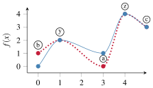
Our ISPH permits assessing the stability of the location of critical points in the pairing. This issue with persistence diagrams was already pointed out by Bendich and Bubenik Bendich15 , who demonstrated that small changes in the critical values of a function—while not drastically changing the persistence diagram itself—may still change the points that are responsible for creating a certain topological feature. The ISPH contains information that may be used to assess the stability of the creators of topological features. To make this more precise, consider the example in Fig. 5. Upon traversing the superlevel sets of both functions, they exhibit the same persistence pairs, namely $(a,z)$, $(b,y)$, and $(c,z)$. Refer to Fig. 4(d) for the corresponding ISPHs. If we perturb the critical point for both functions (indicated by a dashed line), we still get the pairs $(b,y)$ and $(c,z)$ for the stable function. For the unstable function, however, the perturbation results in the pairs $(b,z)$ and $(c,y)$. In this sense, their location is less stable.

We thus define a stability measure for each critical point based on the hierarchy. First, we need to quantify the stability of an edge. Let $e:=\{(\sigma,\tau),(\sigma^{\prime},\tau^{\prime})\}$ be an edge in the ISPH. We define the stability of $e$ to be

$$\operatorname{stab}(e):=\max\left\{|f(\sigma)-f(\sigma^{\prime})|,|f(\tau)-f(\tau^{\prime})|\right\},$$ (5)

which is the minimum amount of perturbation that is required to change the hierarchy in the sense described above. This quantity is also equal to the $\mathrm{L}_{\infty}$-distance between two points in a persistence diagram. We may now extend the stability measure to individual vertices by assigning each vertex $v$ the minimum stability value of its outgoing edges, i.e.,

$$\operatorname{stab}(v):=\min\big{\{}\min\{\operatorname{stab}(e)\mid e=(v,w)\in\mathcal{H}\},\operatorname{pers}(v)\big{\}},$$ (6)

where $w$ ranges over all direct children of $v$. Taking the second minimum ensures that we use the persistence of $v$ if $v$ is a leaf node.

Dissimilarity Measure

Since the ISPH is a directed tree, a straightforward dissimilarity measure is given by tree edit distance Bille05 algorithms. These algorithms attempt to transform two trees into each other by three elementary operations: relabeling a given node, deleting an existing node, and inserting a new node. Given two nodes with corresponding minima–maxima $(c_{1},d_{1})$ and $(c_{2},d_{2})$, respectively, we define the cost for relabeling to be

$$\mathrm{cost}_{1}=\max\big{(}|c_{1}-c_{2}|,|d_{1}-d_{2}|\big{)},$$ (7)

i.e., the $\mathrm{L}_{\infty}$-distance between the two points. Similarly, we define the cost for deleting or inserting a node somewhere else in the hierarchy to be

$$\mathrm{cost}_{2}=\operatorname{pers}(c,d)=|d-c|,$$ (8)

i.e., the persistence of the pair. The choice of these costs is “natural” in the sense that they are also used, e.g., when calculating the bottleneck distance Cohen-Steiner07 between persistence diagrams.

Complexity The tree edit distance has the advantage of being efficiently-solvable via standard dynamic programming techniques. It is thus scalable with respect to the size of the hierarchy—more so than the Wasserstein or bottleneck distances Maria14 ; Tierny18 that are commonly used for comparing persistence diagrams: we have a worst case complexity of $\mathcal{O}\left(n^{2}m\log m\right)$, where $n$ is the number of pairs in the smaller hierarchy, and $m$ is the number of pairs in the larger hierarchy. By contrast, the Wasserstein distance has a time complexity of $\mathcal{O}\left(n^{3}\right)$ (Edelsbrunner10, , p. 196), and we observed large differences in runtime behavior (see Sec. 5).

5 Results

We exemplify some usage scenarios of the ISPH by means of several synthetic and non-synthetic datasets.

5.1 Synthetic Data

(a)

(b)

Figure 6: In contrast to previous approaches, our hierarchy is capable of distinguishing between two peaks that are connected via a third one that is higher 6(a) and a “ridge” of peaks 6(b).

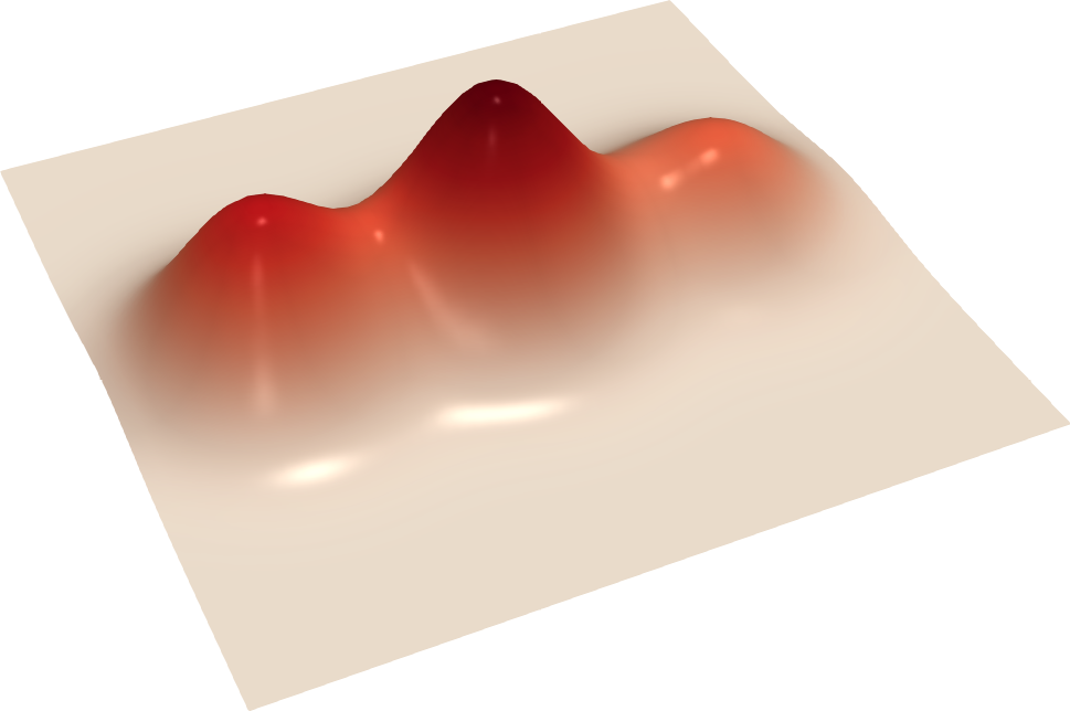
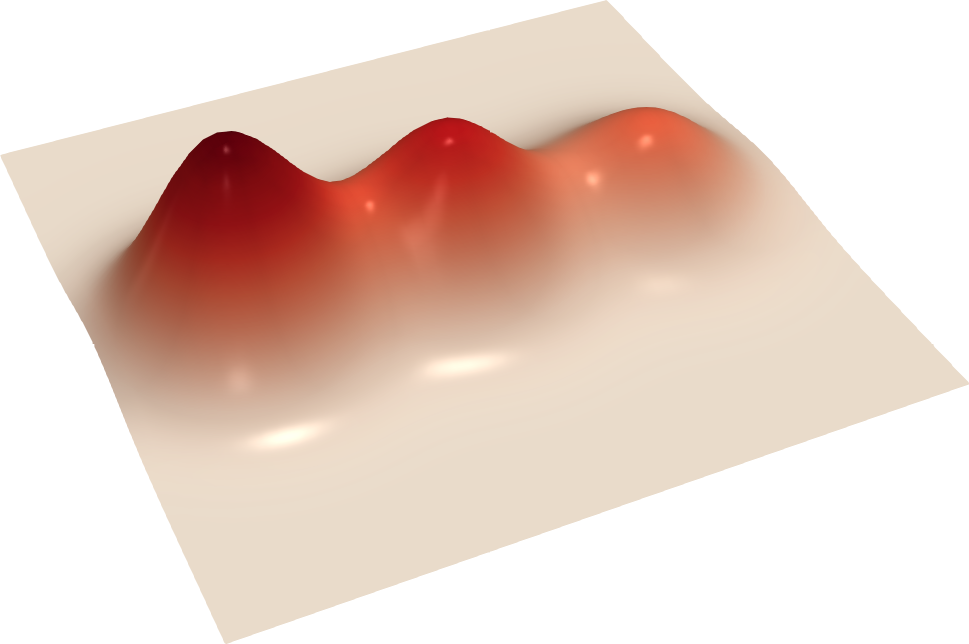
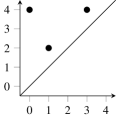
We created two synthetic datasets on a grid with 5,000 cells. Processing each dataset takes approximately $4.5\text{\,}\mathrm{s}$—regardless of whether we calculate the regular persistence hierarchy or the ISPH. Our current implementation leaves lots of room for performance improvements, though. Fig. 6 shows the data together with the resulting hierarchies for the two-dimensional equivalent to the data shown in Fig. 5. We use a standard color map that uses red for large values and white for low values. Notice that the persistence diagrams of both datasets are equal, as well as their regular persistence hierarchies (which we do not show here). Fig. 7(a) depicts the persistence diagrams of the two data sets, colored by their stability values and the ranks (mirrored along the diagonal). Even this summary information gleaned from the ISPH is capable of yielding information to distinguish different datasets.

(a) Persistence diagrams for Fig. 6

(b) Persistence diagrams for Fig. 8

Figure 7: Combined persistence diagrams showing the ranks (upper part) and the stability values (lower part) as colors. Both carry sufficient information to distinguish datasets.

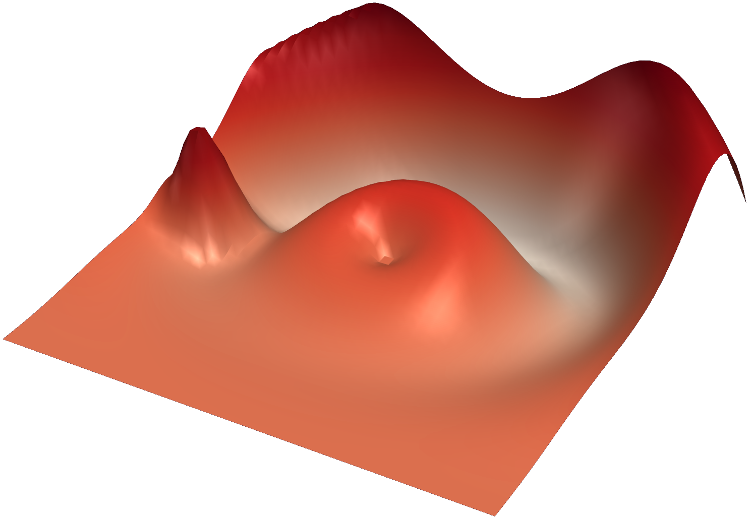
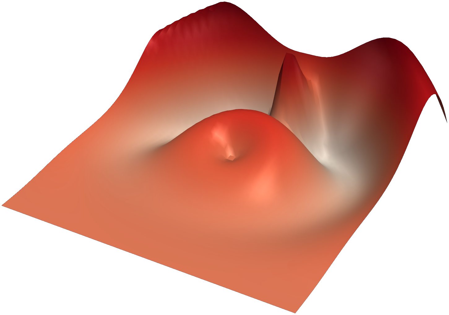
Fig. 8 depicts a more complicated example, mixing peaks and craters. The situation in Fig. 8(b) is less stable because a perturbation of the peak is capable of changing the complete pairing. Since this peak is connected differently in Fig. 8(a), it does not decrease the stability of the global maximum. Note that the location of the peak is allowed to move; as long as it stays on the ridge, as depicted in Fig. 8(b), the ISPH will not change. Likewise, as long as the peak moves along the plateau in the foreground, the ISPH will remain the same as depicted in Fig. 8(a).

(a)

(b)

Figure 8: Depending on the position of a single peak that moves, our hierarchies are different, because the merging behavior of critical points has been changed.

5.2 Climate Data

(a) $t=0$

(b) $t=1$

(c) $t=2$

(d) $t=3$

(e) $t=4$

Figure 9: Climate dataset for $t=0$ (a), as well as some excerpts (box) for subsequent timesteps. We can see that the continent of Africa exhibits a temperature increase for $t=3$ and $t=4$.

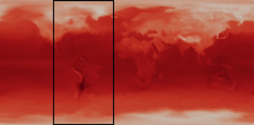
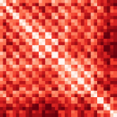
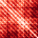
We used time-varying scalar field data (surface temperature) from the German Climate Computing Center (DKRZ). The large size (18,432 positions) and the large number of timesteps (1460) makes comparing these data complicated. Fig. 9 shows an excerpt of the dataset. It exhibits oscillatory behavior because (global) temperature follows a day–night pattern. At the given resolution, a full day–night cycle comprises four timesteps. We would hence expect that the topological dissimilarity between corresponding timesteps is somewhat equal; or, more precisely, we would expect that a pairwise distance matrix depicts the oscillatory behavior that occurs in the data. To assess the capabilities of the dissimilarity measure from Sec. 4.2, we compare it to the Wasserstein distance. We first calculate pairwise distances between the first 36 timesteps of the data. Calculating the Wasserstein distance takes about $2\text{\,}\mathrm{min}$ per pair, hence comparing all 36 pairs takes about $21\text{\,}\mathrm{h}$. Our hierarchy-based dissimilarity measure, by contrast, takes $2.3\text{\,}\mathrm{s}$ for calculating each timestep and approximately $6\text{\,}\mathrm{s}$ to calculate the dissimilarity per pair. The full distance matrix is thus obtained in approximately $1\text{\,}\mathrm{h}$. Fig. 10 depicts the dissimilarity matrices of the first 36 timesteps. We can see that the ISPH distance matrix contains patterns in the minor diagonals, indicating that timesteps $t_{i}$ and $t_{i+4}$ are highly similar. These patterns appear because the corresponding ISPHs are also highly similar, even though the persistence pairs (and thus the persistence diagrams) change over time because the range of temperatures changes. The Wasserstein distance does not exhibit these patterns. We note, however, that the two matrices are highly correlated ($R^{2}\approx 0.95$), showing that for most of the timesteps, both measures yield similar values.

(a) Wasserstein distance

(b) ISPH distance

Figure 10: Dissimilarity matrices comparing the Wasserstein distance and our proposed ISPH distance, which is capable of detecting the oscillatory behavior (minor diagonals) inherent to the data.

6 Conclusion and Future Work

We presented a novel hierarchy that relates persistence pairs with each other. In contrast to earlier work, our hierarchy is better capable of distinguishing certain nesting behaviors, which we demonstrated by means of several example datasets. At present, it is unclear to what extent the persistence hierarchy is an invariant like the rank invariant of multidimensional persistence Carlsson09 . Since the hierarchy changes when the data undergoes certain transformations, it remains to be shown which operations leave it unchanged—a trivial observation is that the hierarchy is invariant with respect to uniform scaling in all critical points. Hence, the development of metrics for matching hierarchies may be beneficial. We only briefly sketched a dissimilarity measure based on labeled trees. By considering the complete connectivity structure of the tree, though, graph kernels such as the random walk kernel Vishwanathan10 could be employed. Furthermore, it would be interesting to analyze how the hierarchy changes when different pairing schemes for critical points are employed, such as the measures proposed by Carr et al. Carr04 .