Persistence Concepts for 2D Skeleton Evolution Analysis

Abstract

In this work, we present concepts for the analysis of the evolution of two-dimensional skeletons. By introducing novel persistence concepts, we are able to reduce typical temporal incoherence, and provide insight in skeleton dynamics. We exemplify our approach by means of a simulation of viscous fingering—a highly dynamic process whose analysis is a hot topic in porous media research.

1 Introduction

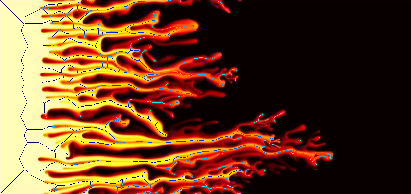
There are many research problems that express themselves more in terms of topological structure than morphology. Typical examples of such processes include electrical discharge, the growth of crystals, and signal transport in networks. In this paper, we address viscous fingering, where the interface between two fluids is unstable and develops highly-dynamic “finger-like” structures. A prominent cause for such structures are setups where a fluid with lower viscosity (Fig. 1(a)–1(c), left) is injected into a fluid with higher viscosity (Fig. 1(a)–1(c), right). To analyze these processes, a straightforward approach employs traditional skeletonization techniques for extracting the topology of each time step independently. Here, we employ iterative thinning thinning1992 . However, like all skeletonization techniques, the resulting skeletons tend to be to temporally incoherent because the extraction is susceptible to small variations and noise. We present persistence concepts to address these issues and provide insight into the underlying processes.

2 Viscous Fingering

Even though the methods described in this paper are generically applicable to time-varying skeletons, we focus our analysis on skeletons that we extracted from viscous fingering processes. The term viscous fingering refers to the formation of structural patterns that appear when liquids of different viscosity are mixed. Under the right conditions, e.g., when water is being injected into glycerine, branch-like structures—the eponymous viscous fingers—begin to appear and permeate through the liquid of higher viscosity. Understanding the formation of these patterns is a prerequisite for the description of many natural processes, such as groundwater flows. Consequently, researchers are interested in setting up simulations that closely match the observations of their experiments.

Since each simulation uses a different set of parameters, summary statistics and comparative visualizations are required in order to assess how well a simulation describes an experiment. As a first step towards analyzing these highly-complex dynamics, we extract skeletons for each time step of a simulation or an experiment. In this paper, we introduce several concepts for assessing the inherent dynamics of these skeletons, permitting a comparative analysis.

Other methods In the context of analyzing viscous fingering, several other techniques exist. An approach by Lukasczyk et al. Lukasczyk17 , for example, uses tracking graphs to visualize the spatio-temporal behavior of such processes. In a more general context, discrete Morse theory could be applied to detect persistent structures in gray-scale images Delgado-Friedrichs15 . The applicability of these approaches hinges on the data quality, however. Our experimental data suffers from a high noise level in which many smaller fingers cannot be easily identified by the other approaches. This is why we decided to focus on conceptually simpler skeletonization techniques for now.

(a) $t=8$

(b) $t=30$

(c) $t=70$

Figure 1: Selected time steps 1(a)–1(c) of a 2D viscous fingering simulation viscousFingeringVideo , with extracted skeleton (overlay). We used a conservative threshold for segmentation to suppress dark-red parts.

Figure 2: The basic pipeline of our approach. The first step, i.e., skeleton extraction, strongly depends on the desired application. Likewise, the analysis step can comprise different diagrams, summary statistics, and goals. Individual parts of the pipeline are replaceable, making our approach highly generic. Our current implementation uses an algorithm by Zhang and Suen Zhang84 for skeleton extraction (Sec. 3.1). The subsequent propagation of creation times between time steps along all branches of the skeleton uses the methods described in the same section. From this extended skeleton, Sec. 3.2 describes how to derive numerous persistence diagrams. Following this, we define multiple activity indicators based on these diagrams in Sec. 3.3. Finally, Sec. 4 presents an analysis of different data sets under different aspects.

3 Overview and Methods

In this paper, we implement a pipeline that comprises the whole range of the analysis process of a series of time-varying skeletons. Fig. 2 shows a schematic illustration and points to the corresponding sections in which individual parts are described. We provide an open-source implementation (in Python) of the pipeline on GitHub. The repository includes all examples, data, and instructions on how to reproduce our experiments. For the analysis of our persistence diagrams, we implemented tools that build upon Aleph, an open-source library for persistent homology calculations. We stress that our implementation is a proof of concept. Its computational bottleneck is the brute-force matching (which could be improved by using an approximate matching algorithm) that is required as a precursor to creation time propagation. More precisely, calculating all matches over all time steps takes between $2\text{\,}\mathrm{h}$ and $6\text{\,}\mathrm{h}$, while the subsequent propagation of creation times takes $82\text{\,}\mathrm{s}$ (example data, $$839\text{\,}\mathrm{px}$\times$396\text{\,}\mathrm{px}$$, 84 time steps), $384\text{\,}\mathrm{s}$ (measured data, $$722\text{\,}\mathrm{px}$\times$1304\text{\,}\mathrm{px}$$, 58 time steps), and $524\text{\,}\mathrm{s}$ (simulation data, $$1500\text{\,}\mathrm{px}$\times$1000\text{\,}\mathrm{px}$$, 37 time steps). Finally, persistence diagram creation requires $100\text{\,}\mathrm{s}$ (example data), $183\text{\,}\mathrm{s}$ (simulation data), and $926\text{\,}\mathrm{s}$ (measured data), respectively. The time for calculating activity indicators (Sec. 3.3), e.g., total persistence, is negligible, as the persistence diagrams only contain a few hundred points. Please refer to Sec. 4 for more information about the individual data sets.

Subsequently, we will first briefly discuss skeleton extraction—both in terms of sets of pixels as well as in terms of graphs. Next, we explain the necessary steps for obtaining information about the “creation time” of pixels and how to propagate said information over all time steps in order to obtain evolution information. Based on this, we derive and exemplify several concepts motivated by topological persistence.

3.1 Skeleton Extraction and Propagation of Pixel Creation Time

Iterative thinning provides skeletons from binary images in a pixel-based format. A sequence of skeletons thus gives rise to a sequence of pixel sets $\mathcal{P}_{0}$, $\mathcal{P}_{1}$, …, $\mathcal{P}_{k}$, each corresponding to a time step $t_{0}$, $t_{1}$, …, $t_{k}$. We employ 8-neighborhood connectivity around each pixel, i.e., the set of all neighbors including the diagonal ones, to convert each pixel set $\mathcal{P}_{i}$ into a graph $\mathcal{G}_{i}$. Depending on the degree $d$ of each vertex in $\mathcal{G}_{i}$, we can classify each pixel as being either a regular point ($d=2$), a start/end point ($d=1$), or a branch point ($d\geq{}3$). This also permits us to define segments formed by connected subsets of regular pixels.

Pixel Matching

Since the skeleton changes over time, we need to characterize the creation time of each pixel, i.e., the time step $t_{i}$ in which it initially appears. Moreover, we want to permit that a pixel “moves” slightly between two consecutive time steps in order to ensure that drifts of the skeleton can be compensated. Our experiments indicate that it is possible to obtain consistent creation times for the pixels based on their nearest neighbors, regardless of whether the simulation suffers from a coarse time resolution or not. Given two time steps $t_{i}$, $t_{i+1}$, we assign every pixel $p\in\mathcal{P}_{i}$ the pixel $p^{\prime}\in\mathcal{P}_{i+1}$ that satisfies

$$p^{\prime}:=\arg\min_{q\in\mathcal{P}_{i+1}}\operatorname{dist}(p,q),$$ (1)

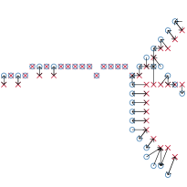
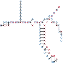
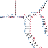
where $\operatorname{dist}(\cdot)$ is the Euclidean distance. Likewise, we assign every pixel in $\mathcal{P}_{i+1}$ its nearest neighbor in $\mathcal{P}_{i}$, which represents a match from $\mathcal{P}_{i+1}$ to $\mathcal{P}_{i}$. This yields a set of directed matches between $\mathcal{P}_{i}$ and $\mathcal{P}_{i+1}$. Each pixel is guaranteed to occur at least once in the set. We refer to matches from $\mathcal{P}_{i}$ to $\mathcal{P}_{i+1}$ as forward matches, while we refer to matches in the other direction as backward matches. A match is unique if the forward and backward match connect the same pair of pixels. Fig. 3 depicts matches for selected time steps and illustrates the movement of pixels.

(a) $t=72$

(b) $t=73$

(c) $t=74$

Figure 3: An excerpt demonstrating matches between two time steps. Some of the pixels of the current time step (blue circles) overlap with pixels from the previous time step (red crosses). We use arrows to indicate forward and backward matches.

Pixel Classification

(a) $t=68$

(b) $t=69$

(c) $t=70$

Figure 4: Classification of all pixels into growth pixels  , decay pixels  , known pixels  , and irregular pixels  . The abrupt appearance 4(b) or disappearance 4(c) of segments is a challenge for skeleton extraction and tracking.

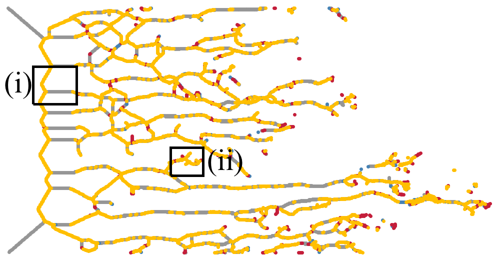
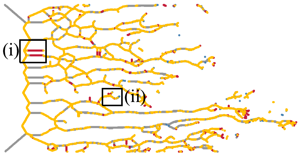
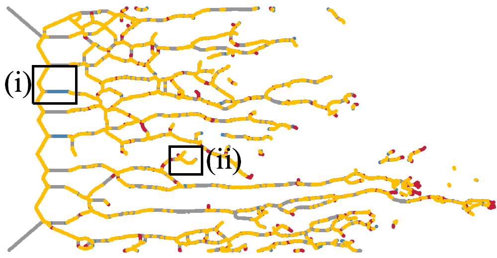
We now classify each pixel in time step $t_{i+1}$ according to the forward matches between $\mathcal{P}_{i}$ and $\mathcal{P}_{i+1}$, as well as the backward matches between $\mathcal{P}_{i}$ and $\mathcal{P}_{i+1}$. We call a pixel known if their match is unique, i.e., there is exactly one forward and one backward match that relate the same pixels with each other. Known pixels are pixels that are already present in a previous time step with a unique counterpart in time step $t_{i+1}$. Similarly, we refer to a pixel in $\mathcal{P}_{i+1}$ as a growth pixel if there is a unique match in $\mathcal{P}_{i}$ and at most one forward match from some other pixel in $\mathcal{P}_{i}$. Growth pixels indicate that new structures have been created in time step $t_{i+1}$, or that existing structures have been subject to a deformation. The counterpart to a growth pixel is a decay pixel in $\mathcal{P}_{i+1}$, which is defined by a unique match in $\mathcal{P}_{i}$ and at most one backward match to the same pixel in $\mathcal{P}_{i}$ from another pixel in $\mathcal{P}_{i+1}$. Decay pixels indicate that a skeleton region has been lost in time step $t_{i+1}$. We refer to all other pixels as irregular. In our experiments, irregular pixels, which are caused by small shifts between consecutive time steps, comprise about 60% of all pixels. As we subsequently demonstrate, we are able to assign consistent creation times despite the prevalence of irregular pixels. Fig. 4 depicts classified pixels for consecutive time steps. It also demonstrates that skeletons may be temporally incoherent: pixels in region (i) only exist for a single time step, forming long but short-lived segments. Pixels in region (ii), by contrast, form short but long-lived segments. We want to filter out segments in region (i), while keeping segments in region (ii) intact. This requires knowledge about pixel creation times.

Propagating Creation Times

Initially, each pixel in $\mathcal{P}_{0}$ is assigned a creation time of $0$. Next, we classify the pixels in each pair of consecutive time steps $t_{i}$ and $t_{i+1}$ as described above. For known pixels, we re-use the creation time of $t_{i}$. For growth pixels, we distinguish two different cases: (i) If a growth pixel in time step $t_{i+1}$ is not the target of a forward match from time step $t_{i}$, we consider it to be a new pixel and hence assign it a creation time of $t_{i+1}$. (ii) Else, we re-use the creation time just as for known pixels. This procedure ensures that we are conservative with assigning “new” creation times; it turns out that a small number of growth pixels with increased creation times is sufficient for propagating time information throughout the data. For all other types of pixels, we assign them the minimum of all creation times of their respective matches from $\mathcal{P}_{i}$, ignoring the direction of the matching. Again, this is a conservative choice that reduces the impact of noise in the data.

(a) $t=68$

(b) $t=69$

(c) $t=70$

Figure 5: Propagated age per pixel, using a white–red color map. The skeleton inconsistencies in region (i) impede the temporal coherence of neighboring pixels.

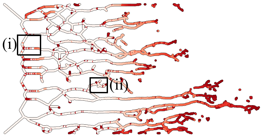
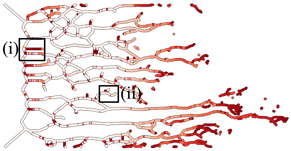
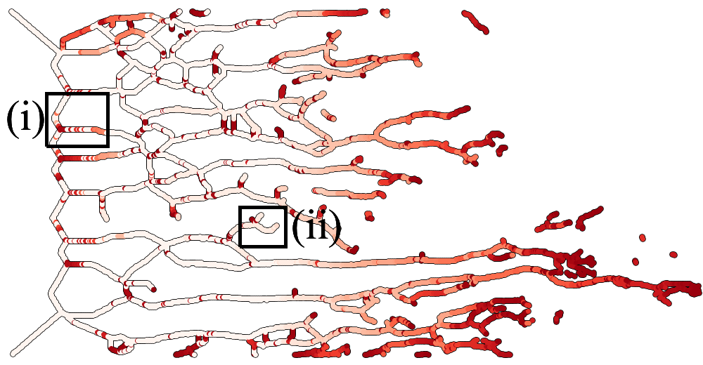
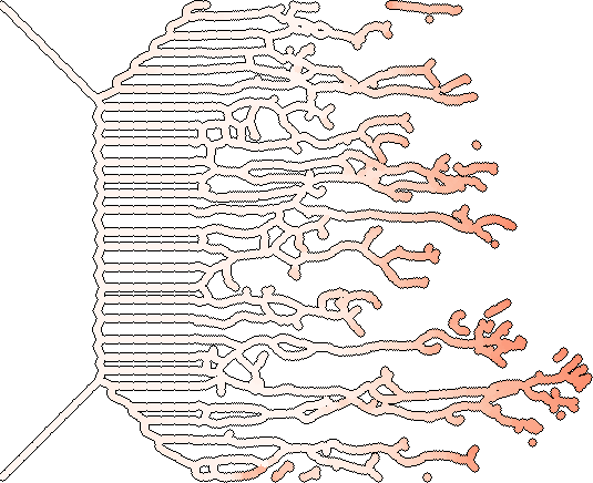
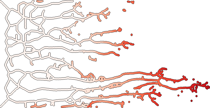
Thus, every pixel in every time step has been assigned a creation time. This time refers to the first time step in which the pixel was unambiguously identified and appeared. By propagating the creation time, we ensure that skeletons are allowed to exhibit some movement between consecutive time steps. Fig. 5 depicts the creation times for several time steps. For temporally coherent skeletons, recent creation times (shown in red) should only appear at the end of new “fingers”. We can see that the brief appearance of segments causes inconsistencies. Ideally, the creation time of pixels should vary continuously among a segment.

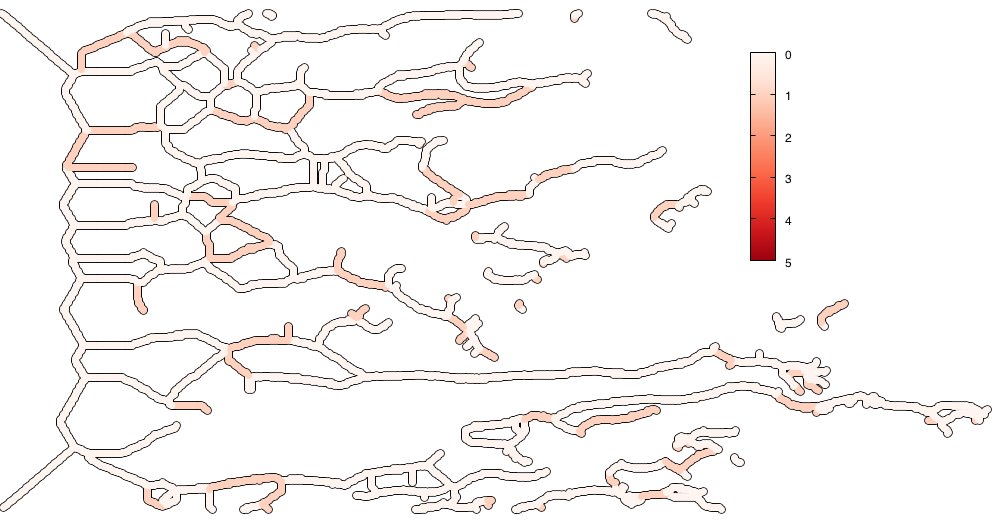
Improving temporal coherence To improve temporal coherence, i.e, creation times of adjacent pixels, we observe that inconsistencies are mainly caused by a small number of growth pixels along a segment. These are a consequence of a “drift” in pixel positions over subsequent time steps, which our naive matching algorithm cannot compensate for. A simple neighborhood-based strategy is capable of increasing coherence, though: for each growth pixel, we evaluate the creation times in its $8$-neighborhood. If more than 50% of the neighbors have a different creation time than the current pixel, we replace its creation time by the mode of its neighbors’ creation times. This strategy is reminiscent of mean shift smoothing Comaniciu02 . Fig. 6 compares the original and improved creation times for two time steps. Ideally, all segments should exhibit a gradient-like behavior, indicating that their structures have been expanded continuously. We see that this is only true for the longest segments. Erroneous creation times are an inevitable byproduct of instabilities in skeleton extraction, which can be mitigated through persistence-based concepts.

(a) $t=42$ (no coherence)

(b) $t=84$ (no coherence)

(c) $t=42$ (coherence)

(d) $t=84$ (coherence)

Figure 6: Pixel creation times at two selected time steps. Recent creation times are shown in shades of red. We can see that the “front” of the fingers is always recent, while the oldest structures have been created at the very beginning. This example also demonstrates how the temporal coherence of creation times can be improved.

3.2 Persistence Concepts

Persistence is a concept introduced by Edelsbrunner et al. Edelsbrunner10 ; Edelsbrunner02 ; Edelsbrunner06 . It yields a measure of the range (or scale) at which topological features occur in data and is commonly employed to filter or simplify complex multivariate data sets Rieck12 . For skeletons, i.e., graphs, the standard topological features are well known, comprising connected components and cycles. While these features are useful in classifying complex networks Carstens13 , for example, they do not provide sufficient information about skeleton evolution processes because they cannot capture the growth of segments. Hence, instead of adopting this viewpoint, we derive several concepts that are inspired by the notion of persistence. A crucial ingredient for this purpose is the availability of creation times for every pixel in every time step.

Branch Inconsistency

Using the graph $\mathcal{G}_{i}$ for a time step $t_{i}$, we know which pixels are branch points, i.e., points where multiple segments meet. Let $c_{b}$ be the creation time of such a branch point, and let $c_{1}$, $c_{2}$, …refer to the creation times of the first adjacent point along each of the segments meeting at the branch point. We define the branch inconsistency for each branch–segment pair as $|c_{i}-c_{b}|$, and we refer to the diagram formed by the points $(c_{b},c_{i})$ as the branch persistence diagram. The number of points in the branch inconsistency diagram indicates how many new branches are being created in one time step. Moreover, it can be used to prune away undesired segments in a skeleton: if the branch inconsistency of a given segment is large, the segment is likely an artifact of the skeletonization process—thinning algorithms often create segments that only exist for a single time step. Overall, those segments thus have a late creation time. In contrast to the persistence diagrams in topological data analysis, where closeness to the diagonal indicates noise, here, points that are away from the diagonal correspond to erroneous segments in the data. Points below the diagonal are the result of inconsistent creation times for some segments—a branch cannot be created before its branch point.

(a) Branch inconsistency

(b) Skeleton

(c) Skeleton, filtered

Figure 7: Branch inconsistency diagram and branch inconsistency values on the skeleton for $t=69$. The diagram indicates that most branches are temporally coherent. Some of them are removed from the diagonal (or below the diagonal), which may either indicate inconsistencies in skeleton tracking or cycles. Removing segments with a branch inconsistency $\geq 5$ (red dots in the diagram, dark red segments in the skeleton) can be used to filter the skeleton.

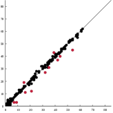
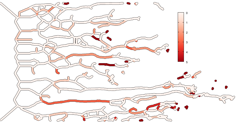
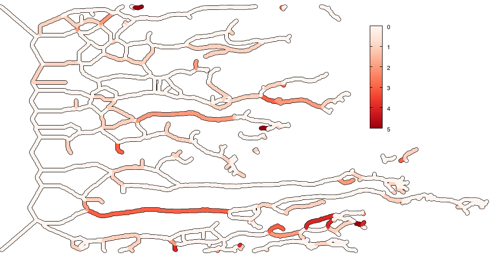
Fig. 7 shows the branch inconsistency diagram and colored skeletons for $t=69$. It also depicts how to filter segments with a large branch inconsistency, which already decreases the number of noisy segments. Please refer to the accompanying video for all branch inconsistency values.

Age Persistence

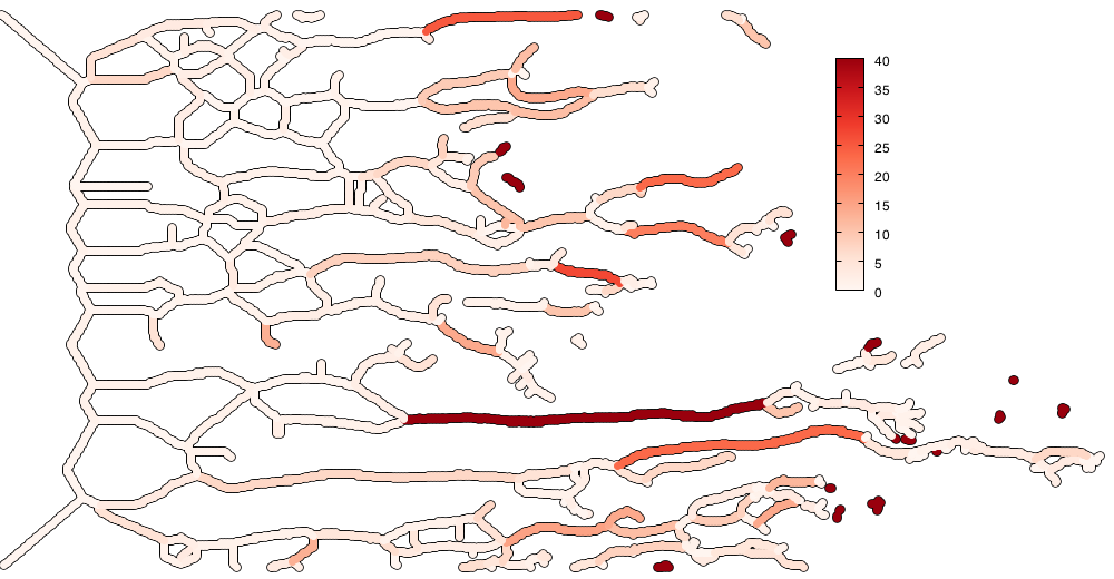
Analogously to branch inconsistency, we obtain an age persistence diagram for each branch–segment pair when we use the maximum creation time of points along each segment. Age persistence is capable of measuring whether a segment is young or old with respect to its branch point. Here, the “persistence” of each point is an indicator of how much the skeleton grows over multiple time steps: if segments stagnate, their points remain at the same distance from the diagonal. If segments continue to grow, however, their points will move away from the diagonal.

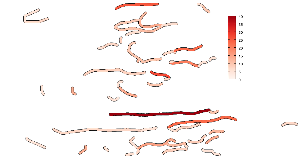
Fig. 8 shows the age persistence diagram and the age persistence values on the skeleton for $t=69$. The filtered skeleton only contains the most active segments, which facilitates tracking. We can combine branch inconsistency and age persistence to remove fewer segments than in Fig. 7(c). For example, we could remove segments that correspond to points below the diagonal of the branch inconsistency diagram and keep those for which both branch inconsistency and age persistence are high. These segments commonly correspond to cycles that were formed during the evolution of the skeleton. An isolated analysis of branch inconsistency is unable to detect them. Fig. 9 depicts the results of such a combined filtering operation.

(a) Age persistence

(b) Skeleton

(c) Skeleton, filtered

Figure 8: Age persistence diagram and age persistence values on the skeleton for $t=69$. Numerous segments towards the “front” of the fingers appear to be active here. Removing all segments whose age persistence is $\leq 5$ (red points in the diagram) leaves us with the most active segments.

(a)

(b)

Figure 9: 9(a) Filtering segments using branch inconsistency may destroy longer segments. 9(b) If we combine both branch inconsistency and age persistence, keeping only those segments whose age persistence is high or whose branch inconsistency is low, we can improve the filter results by removing noisy segments while keeping more cycles intact.

Growth Persistence

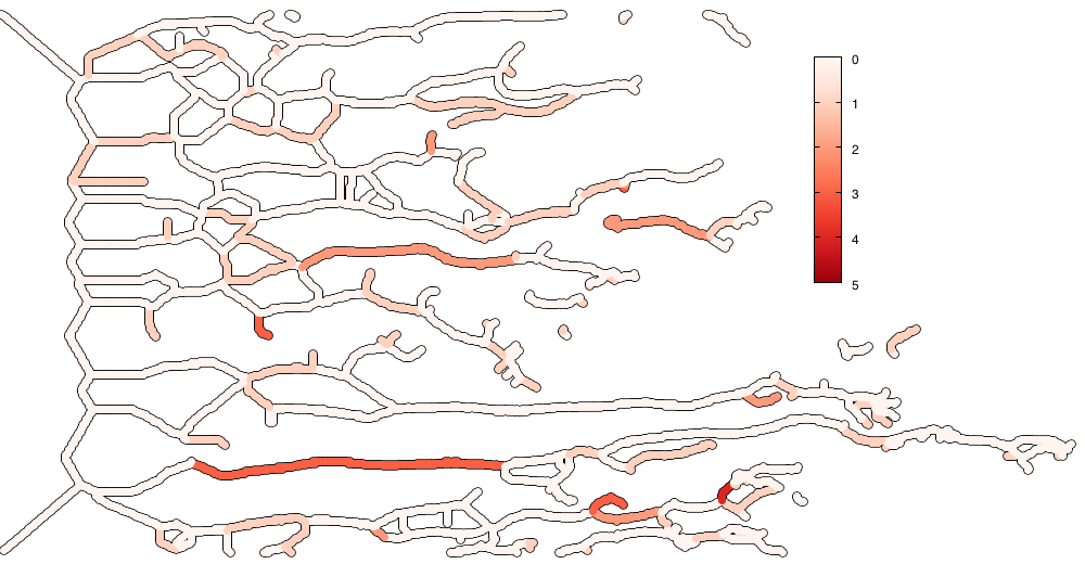
We define the growth persistence of a segment in $\mathcal{G}_{i}$ as the difference between the maximum creation time $t_{\max}$ of its pixels and the current time step $t_{i}$. Intuitively, this can be thought of performing “time filtration” of a simplicial complex, in which simplices may be created and destroyed (notice that such a description would require zigzag persistence for general simplicial complexes). A small value in this quantity indicates that the segment is still growing, while larger values refer to segments that stagnate. Growth persistence is useful to highlight segments that are relevant for tracking in viscous fingering processes. In contrast to the previously-defined persistence concepts, growth persistence is only defined per segment and does not afford a description in terms of a persistence diagram. Fig. 10 depicts the growth persistence of several time steps. Red segments are growing fast or have undergone recent changes, such as the creation of cycles. A low branch persistence in segments, coupled with a low growth persistence corresponds to features that are “active” during skeleton evolution. Please refer to the accompanying video for the evolution of growth persistence.

(a) $t=21$

(b) $t=42$

(c) $t=84$

Figure 10: Growth persistence values. Red segments are highly active in the evolution of the skeleton. In this example, red segments are mostly those that are at the tips of individual “fingers”.

3.3 Activity Indicators

In order to capture the dynamics of skeleton evolution, we require a set of activity indicators. They are based on the previously-defined concepts and can be used to quickly summarize a time series of evolving skeletons.

Total Persistence

There are already various summary statistics for persistence diagrams. The 2^nd-order total persistence $\operatorname{pers}(\mathcal{D})$ Cohen-Steiner10 of a persistence diagram $\mathcal{D}$ is defined as

$$\operatorname{pers}(\mathcal{D})_{2}:=\left(\sum_{(c,d)\in\mathcal{D}}\operatorname{pers}^{2}(c,d)\right)^{\frac{1}{2}},$$ (2)

i.e., the sum of powers of the individual persistence values (i.e. coordinate differences) of the diagram. Total persistence was already successfully used to assess topological activity in multivariate clustering algorithms Rieck16a .

Here, the interpretation of total persistence depends on the diagram for which we compute it. Recall that in a branch inconsistency diagram, points of high “persistence” indicate inconsistencies in branching behavior. Total persistence thus helps detect anomalies in the data; see Fig. 12 for a comparison of total branch persistence in different data sets. For age persistence, by contrast, high persistence values show that a skeleton segment is still actively changing. The total age persistence hence characterizes the dynamics of the data, e.g., whether many or few segments are active at each time step. Fig. 14 depicts a comparison of total age persistence in different data sets.

Vivacity

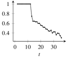
We also want to measure the “vivacity” of a viscous fingering process. To this end, we employ the growth persistence values. Given a growth threshold $t_{\mathrm{G}}$, we count all growth pixels with $\operatorname{\operatorname{pers}_{G}}\leq t_{\mathrm{G}}$ and divide them by the total number of pixels in the given time step. This yields a measure of how much “mass” is being created at every time step of the process. Similarly, we can calculate vivacity based on segments in the data. However, we found that this does not have a significant effect on the results, so we refrain from showing the resulting curves. Fig. 15 depicts vivacity curves for different data sets with $t_{\mathrm{G}}=10$.

4 Analysis

(a) Measured data set, $t=33$

(b) Simulation data set, $t=26$

Figure 11: Selected still images from the two remaining data sets. The measured data in 11(a) exhibits artifacts (parallel lines) that are caused by the experimental setup. The simulation data 11(b), by contrast, does not contain any noise.

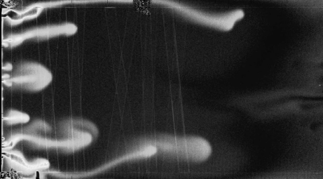
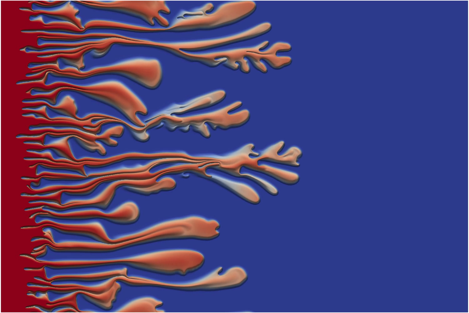
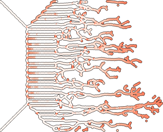
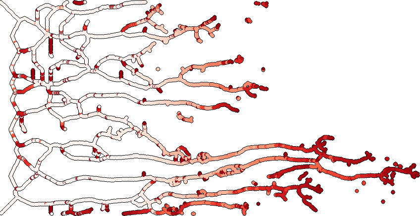
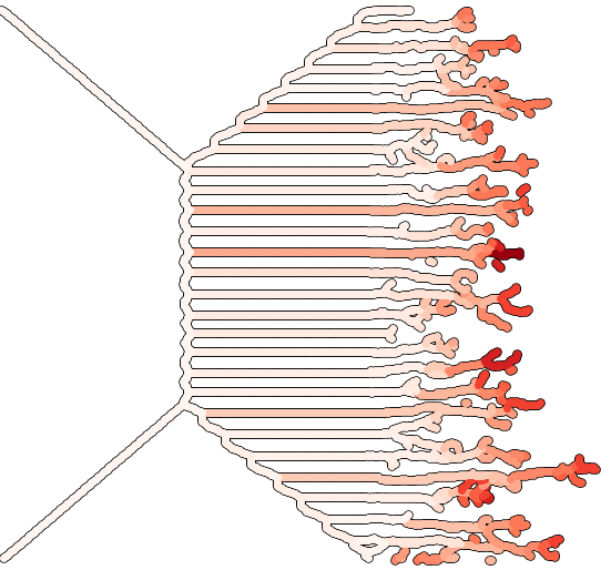
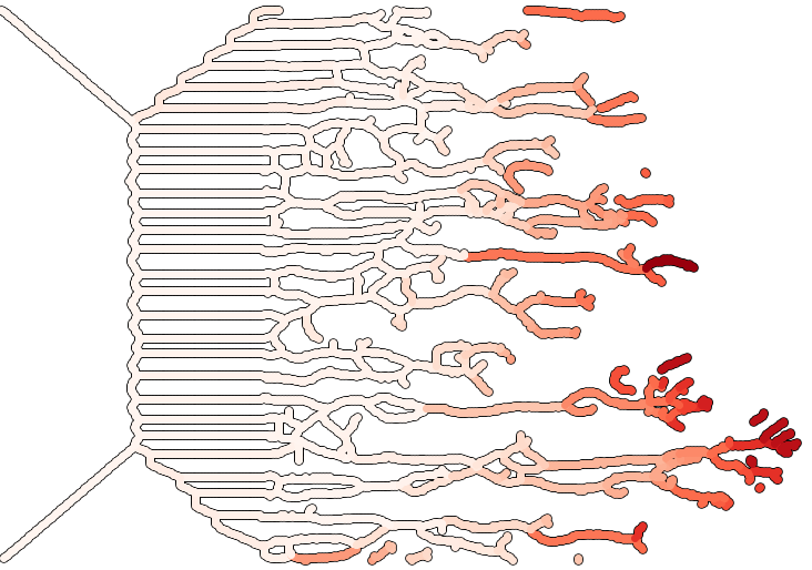
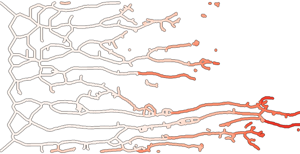
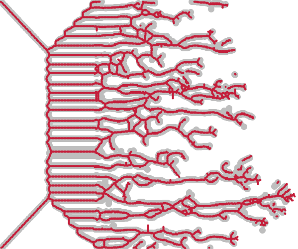
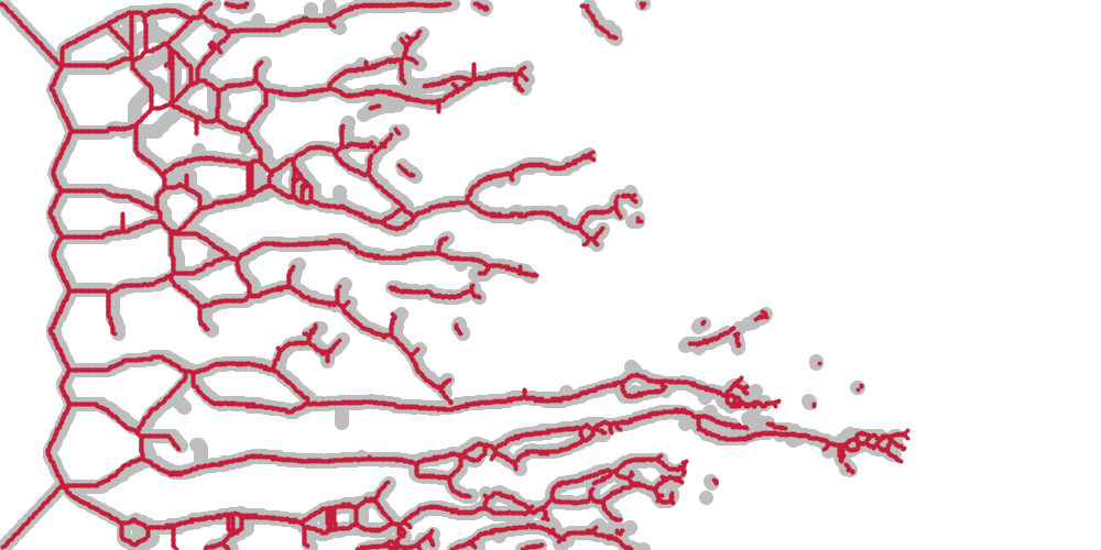
Having defined a variety of persistence-based concepts, we now briefly discuss their utility in analyzing time-varying skeleton evolution. In the following, we analyze three different data sets: (i) the example data set that we used to illustrate all concepts, (ii) a measured data set, corresponding to a slowly-evolving viscous fingering process, (iii) and a simulation of the example data set. Fig. 11 depicts individual frames of the latter two data sets. The measured data set is characterized by a viscous fingering process whose fingers evolve rather slowly over time. Moreover, this experiment, which was performed over several days, does not exhibit many fingers. The simulation data, by contrast, aims to reproduce the dynamics found in the example data set; hence, it contains numerous fast-growing fingers. Please refer to the accompanying videos for more details.

(a) Example

(b) Measured

(c) Simulation

Figure 12: A comparison of total persistence of the branch inconsistency diagram for three different data sets. The first data set 12(a) exhibits more anomalies; these are indicated by “jumps” in the total persistence curve.

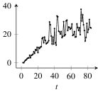
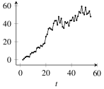
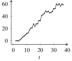
Anomaly detection To detect anomalies in skeleton extraction and tracking, we calculate the total persistence of the branch inconsistency diagram. Fig. 12 compares the values for all data sets. We observe that the example data set, Fig. 12(a), exhibits many “jumps” in branch inconsistency. These are time steps at which the skeleton (briefly) becomes inconsistent, e.g., because a large number of segments disappears, or many small cycles are created. At $t=43$ and $t=72$ (both local maxima in the diagram), for example, we observe changes in the number of cycles as well as the appearance of numerous segments of various lengths, which makes it harder to assign consistent creation times according to Sec. 3.1. Fig. 13 depicts the changes in skeleton topology at these time steps. The other two data sets contain fewer anomalies. For the measured data, this is caused by lower propagation velocities and fewer “fingers” in the data. For the simulation data, this is due to a better separation of individual fingers, caused by the synthetic origin of the data.

(a) $t=43$

(b) $t=72$

Figure 13: Comparing the previous (gray) and the current time step (red) based on total persistence of the branch inconsistency diagram helps uncover problems with skeleton extraction.

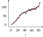
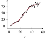
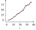
Active branches We use total age persistence to assess the rate at which existing branches move. Fig. 14 compares the data sets, showing both the original total age persistence values as well as a smooth estimate, obtained by fitting Bézier curves Farin93 to the sample points. In Fig. 14(c), the simulated origin of the data is evident: while the other data sets exhibit changes in the growth rate of total age persistence, the simulation data clearly exhibits almost constant growth. Moreover, we observe that the measured data in Fig. 14(b) has a period of constant growth for $t\in[20,40]$, while the example data displays a slightly diminished growth rate for $t\in[25,65]$, only to pick up at the end. Age persistence may thus be used to compare the characteristics of different skeleton evolution processes.

(a) Example

(b) Measured

(c) Simulation

Figure 14: A comparison of total age persistence for the three different data sets, along with a smooth estimate for showing trends.

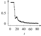
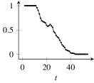
Quantifying dissimilarity To quickly quantify the dissimilarity between different curves, e.g., the vivacity curves that we defined in Sec. 3.3, we can use dynamic time warping Berndt94 , a technique from dynamic programming that is able to compensate for different sampling frequencies and different simulation lengths. Fig. 15 depicts the vivacity curves of the data sets. We can see that the measured data in Fig. 15(b) is characterized by a slower process in which new mass is continuously being injected to the system. Hence, its vivacity does not decrease steeply as that of the example data in Fig. 15(a). The vivacity curve for the simulation, shown in Fig. 15(c), appears to differ from the remaining curves. As a consequence, we can use these curves in visual comparison tasks and distinguish between different (measured) experiments and simulations. The dynamic time warping distance helps quantify this assumption. We have $\operatorname{dist}(a,b)\approx 442$, $\operatorname{dist}(a,c)\approx 1135$, and $\operatorname{dist}(b,c)\approx 173$. This indicates that the characteristics of the simulation in Fig. 15(c) differ from those found in a real-world viscous fingering process, shown in Fig. 15(a), while being reasonably close to another measured experiment, which is depicted by Fig. 15(b). Vivacity curves may thus be used for parameter tuning of simulations in order to obtain better approximations to measured data.

(a) Example

(b) Measured

(c) Simulation

Figure 15: Vivacity curves (pixel-based) for the three different data sets. At a glance, the curves permit comparing the dynamics of each process. The sampling frequencies are different, necessitating the use of dynamic time warping.

5 Conclusion

Driven by the need for a coherent analysis of time-varying skeletons, we developed different concepts inspired by topological persistence in this paper. We showed how to improve the consistency of tracking algorithms between consecutive time steps. Moreover, we demonstrated the utility of our novel concepts for different purposes, including the persistence-based filtering of skeletons, anomaly detection, and characterization of dynamic processes.

Nonetheless, we envision numerous other avenues for future research. For example, the propagation velocity of structures in the data may be of interest in many applications. We also plan to provide a detailed analysis of viscous fingering, including domain expert feedback, and extend persistence to physical concepts within this context. More generally, our novel persistence-inspired concepts can also be used in other domains, such as the analysis of motion capture data (which heavily relies on skeletonization techniques) or time-varying point geometrical point clouds, for which novel skeletonization techniques were recently developed Kurlin15 .

References

- (1) Viscous fingering displacement. https://www.youtube.com/watch?v=NZEB8tQ3eOM
- (2) Berndt, D.J., Clifford, J.: Using dynamic time warping to find patterns in time series. Tech. Rep. WS-94-03, AAAI (1994)
- (3) Carstens, C., Horadam, K.: Persistent homology of collaboration networks. Mathematical Problems in Engineering 2013, 815,035:1–815,035:7 (2013)
- (4) Cohen-Steiner, D., Edelsbrunner, H., Harer, J., Mileyko, Y.: Lipschitz functions have -stable persistence. Foundations of Computational Mathematics 10(2), 127–139 (2010)
- (5) Comaniciu, D., Meer, P.: Mean shift: a robust approach toward feature space analysis. IEEE Transactions on Pattern Analysis and Machine Intelligence 24(5), 603–619 (2002)
- (6) Delgado-Friedrichs, O., Robins, V., Sheppard, A.: Skeletonization and partitioning of digital images using discrete Morse theory. IEEE Transactions on Pattern Analysis and Machine Intelligence 37(3), 654–666 (2015)
- (7) Edelsbrunner, H., Harer, J.: Computational topology: An introduction. AMS (2010)
- (8) Edelsbrunner, H., Letscher, D., Zomorodian, A.J.: Topological persistence and simplification. Discrete & Computational Geometry 28(4), 511–533 (2002)
- (9) Edelsbrunner, H., Morozov, D., Pascucci, V.: Persistence-sensitive simplification of functions on 2-manifolds. In: Proceedings of the 22nd Annual Symposium on Computational Geometry, pp. 127–134. ACM Press, New York, NY, USA (2006)
- (10) Farin, G.: Curves and surfaces for computer-aided geometric design: A practical guide, 3rd edn. Elsevier (1993)
- (11) Kurlin, V.: A one-dimensional homologically persistent skeleton of an unstructured point cloud in any metric space. Computer Graphics Forum 34(5), 253–262 (2015)
- (12) Lam, L., Lee, S.W., Suen, C.Y.: Thinning methodologies—a comprehensive survey. IEEE Transactions on Pattern Analysis and Machine Intelligence 14(9), 869–885 (1992)
- (13) Lukasczyk, J., Aldrich, G., Steptoe, M., Favelier, G., Gueunet, C., Tierny, J., Maciejewski, R., Hamann, B., Leitte, H.: Viscous fingering: A topological visual analytic approach. In: Physical Modeling for Virtual Manufacturing Systems and Processes, Applied Mechanics and Materials, vol. 869, pp. 9–19 (2017)
- (14) Rieck, B., Leitte, H.: Exploring and comparing clusterings of multivariate data sets using persistent homology. Computer Graphics Forum 35(3), 81–90 (2016)
- (15) Rieck, B., Mara, H., Leitte, H.: Multivariate data analysis using persistence-based filtering and topological signatures. IEEE Transactions on Visualization and Computer Graphics 18(12), 2382–2391 (2012)
- (16) Zhang, T.Y., Suen, C.Y.: A fast parallel algorithm for thinning digital patterns. Communications of the ACM 27(3), 236–239 (1984)