Persistent Intersection Homology for the Analysis of Discrete Data

Abstract

Topological data analysis is becoming increasingly relevant to support the analysis of unstructured data sets. A common assumption in data analysis is that the data set is a sample—not necessarily a uniform one—of some high-dimensional manifold. In such cases, persistent homology can be successfully employed to extract features, remove noise, and compare data sets. The underlying problems in some application domains, however, turn out to represent multiple manifolds with different dimensions. Algebraic topology typically analyzes such problems using intersection homology, an extension of homology that is capable of handling configurations with singularities. In this paper, we describe how the persistent variant of intersection homology can be used to assist data analysis in visualization. We point out potential pitfalls in approximating data sets with singularities and give strategies for resolving them.

1 Introduction

The manifold hypothesis is a traditional assumption for the analysis of multivariate data. Briefly put, it assumes that the input data are a sample of some manifold $\mathds{M}$, whose intrinsic dimension $d$ is much smaller than the ambient dimension $D$. Typical examples of this assumption are found in dimensionality reduction algorithms Roweis00 ; Tenenbaum00 . For certain applications, such as image analysis Donoho05 or image recognition Hinton97 , we already know this hypothesis to be true—at least with respect to the models that are often used to describe such data. For other applications, there are strategies Fefferman16 ; Narayanan10 for testing this hypothesis provided that a sufficient number of samples is available.

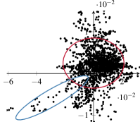
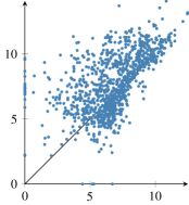
The practice of multivariate data analysis seems to suggest something else, though: Carlsson Carlsson14 , for example, remarks that many real-world data sets exhibit a central “core” structure, from which different “flares” emanate. Figure 1 illustrates this for a simple 2D data set, generated from 2-year growth rates of Standard & Poor’s 500 vs. the U.S. CPI. This structure is irreconcilable with the structure of a single manifold. Novel data analysis algorithms such as Mapper Singh07 account for this fact by not making any assumptions about manifold structures and attempting to fit data in a local manner—a strategy that is also employed in low-dimensional manifold learning Saul03 .

In this paper, we argue that some real-world data sets require special tools to assess their structure. Just as persistent homology Edelsbrunner10 ; Edelsbrunner14 was originally developed to analyze samples from spaces that are supposed to have the structure of a manifold, we need a special tool to analyze spaces for which this assumption does not hold. More precisely, we will tackle the task of analyzing spaces that are composed of different manifolds (with possibly varying dimensions) using intersection homology Kirwan06 and persistent intersection homology Bendich09 ; Bendich11 . To make it accessible to a wider community of researchers, we devote a large portion of this paper to explaining the theory behind persistent intersection homology. Furthermore, we discuss implementation details and present an open-source framework for its calculation. We also describe pitfalls in “naive” applications of persistent intersection homology and develop strategies to resolve them.

(a) Data set

(b) Persistence diagram

Figure 1: LABEL:sub@sfig:Data_set_example The structure of a central “core” with “flares” emanating from it appears in many data sets (here, 2-year growth rates of Standard & Poor’s 500 vs. the U.S. CPI with the core shown in red and one example flare shown in blue). LABEL:sub@sfig:Persistence_diagram_example The corresponding persistence diagram shows topological features in dimension zero (red) and dimension one (blue).

2 Background

We first explain the mathematical tools required to describe spaces that are not composed of a single manifold, but of multiple ones. Next, we introduce (persistent) intersection homology, give a brief algorithm for its computation, and describe how to use it to analyze real-world data sets.

2.1 Stratifications

(a)

(b)

Figure 2: LABEL:sub@fig:Pinched_torus The “pinched torus” is a classical example of an object that is not a manifold but composed of parts that are manifolds, provided the singular point that is caused by the “pinch” is ignored. LABEL:sub@fig:Pinched_torus_curvature The singular point is readily visible when calculating mean curvature estimates.

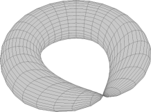
Stratifications are a way of describing spaces that are not a manifold per se, but composed of multiple parts, each of which is a manifold. A common example of such a space is the “pinched torus”, which is obtained by collapsing (i.e., pinching) one minor ring of the torus to a single point. Figure LABEL:fig:Pinched_torus depicts an example. The neighborhood of the pinch point is singular because it does not satisfy the conditions of a manifold: it does not have a neighborhood that is homeomorphic to a ball. If we remove this singular point, however, the remaining space is just a (deformed) cylinder, i.e., a manifold. Permitting the removal of certain parts of a space may thus be beneficial to describe the manifolds it is composed of. This intuition leads to the concept of stratifications.

Let $X\subseteq{}^{n}$ be a topological space. A topological stratification of $X$ is a filtration of closed subspaces

$$\emptyset\subseteq X_{-1}\subseteq X_{0}\subseteq X_{1}\subseteq\dots\subseteq X_{d-1}\subseteq X_{d}=X,$$ (1)

such that for each $i$ and every point $x\in X_{i}\setminus X_{i-1}$ there is a neighborhood $U\subseteq X$ of $x$, a compact $(n-1-i)$-dimensional stratified topological space V, and a filtration-preserving homeomorphism $U\simeq{}^{i}\times CV$, where $CV$ denotes the open cone on $V$, i.e., $CV:=V\times[0,1)/(V\times\{0\})$. We refer to $X_{i}\setminus X_{i-1}$ as the $i$-dimensional stratum of $X$. Notice that it is always a (smooth) manifold, even though the original space might not be a manifold. Hence, this rather abstract definition turns out to be a powerful description for a large family of spaces. There are some stratifications with special properties that are particularly suited for analyzing spaces. Goresky and MacPherson Goresky80 , the inventors of intersection homology, suggest using a stratification that satisfies $X_{d-1}=X_{d-2}$ so that the $(d-1)$-dimensional stratum is empty, i.e., $X_{d-1}\setminus X_{d-2}=\emptyset$.

2.2 Homology and Persistent Homology

Prior to introducing (persistent) intersection homology, we briefly describe simplicial homology and its persistent counterpart. Given a $d$-dimensional simplicial complex $\mathrm{K}$, the chain groups $\{C_{0}$, …, $C_{d}\}$ contain formal sums (simplicial chains) of simplices of a given dimension. A boundary operator $\partial_{p}\colon C_{p}\to C_{p-1}$ satisfying $\partial_{p-1}\circ\partial_{p}=0$ (i.e., a closed boundary does not have a boundary itself) then permits us to create a chain complex from the chain groups. This results in two subgroups, namely the cycle group $Z_{p}:=\ker\partial_{p}$ and the boundary group $B_{p}:=\operatorname{im}\partial_{p+1}$, from which we obtain the $p$^th homology group as

$$H_{p}:=Z_{p}/B_{p},$$ (2)

where the $/$-operator refers to the quotient group. Intuitively, elements in the cycle group $Z_{p}$ constitute sets of simplicial chains that do not have a boundary, while elements in the boundary group $B_{p}$ are the boundaries of higher-dimensional simplices. By removing these in the definition of the homology group, we obtain a group that describes high-dimensional “holes” in $\mathrm{K}$.

Homology is a powerful tool to discriminate between different triangulated topological spaces. It is common practice to use the Betti numbers $\beta_{p}$, i.e., the ranks of the homology groups, to obtain a signature of a space. In practice, the Betti numbers turn out to be highly susceptible to noise, which prompted the development of persistent homology Edelsbrunner10 . Its basic premise is that the simplicial complex $\mathrm{K}$ is associated with a filtration,

$$\emptyset=\mathrm{K}_{0}\subseteq\mathrm{K}_{1}\subseteq\dots\subseteq\mathrm{K}_{n-1}\subseteq\mathrm{K}_{n}=\mathrm{K},$$ (3)

where each $\mathrm{K}_{i}$ is typically assigned a function value, such as a distance. The filtration induces a homomorphism of the corresponding homology groups, i.e., $f_{p}^{i,j}\colon H_{p}(\mathrm{K}_{i})\to H_{p}(\mathrm{K}_{j})$, leading to the definition of the $p$^th persistent homology group $H_{p}^{i,j}$ for two indices $i\leq j$ as

$$H_{p}^{i,j}:=Z_{p}\left(\mathrm{K}_{i}\right)/\left(B_{p}\left(\mathrm{K}_{j}\right)\cap Z_{p}\left(\mathrm{K}_{i}\right)\right).$$ (4)

This group contains all the homology classes of $\mathrm{K}_{i}$ that are still present in $\mathrm{K}_{j}$. It is possible to keep track of all homology classes within the filtration.

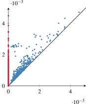
The calculation of persistent homology results in a set of pairs $(i,j)$, which denote a homology class that was created in $\mathrm{K}_{i}$ and destroyed (vanished) in $\mathrm{K}_{j}$. Letting $f_{i}$ denote the associated function value of $\mathrm{K}_{i}$, these pairs are commonly visualized in a persistence diagram Cohen-Steiner07 as $(f_{i},f_{j})$. The distance of each pair to the diagonal, measured in the $\mathrm{L}_{\infty}$-norm, is referred to as the persistence of a topological feature. It is now common practice in topological data analysis to use persistence to separate noise from salient features in real-world data sets Edelsbrunner10 ; Edelsbrunner14 . Figure 1b shows the persistence diagram of an example data set. Since the data set, shown in Figure 1a, appears to be a “blob”, the persistence diagram, as expected, contains few topological features of high persistence in both dimensions.

2.3 Intersection Homology and Persistent Intersection Homology

Despite its prevalence in data analysis, persistent homology exhibits some limitations. In the context of this paper, we are mostly concerned with its lack of duality for non-manifold data sets, and with its inability to detect topological features of data sets consisting of multiple manifolds. Recall that for a $d$-manifold, Poincaré duality means that the Betti numbers satisfy $\beta_{k}=\beta_{d-k}$. While it is possible to extend persistent homology to obtain something similar for manifolds Cohen-Steiner09 ; Silva11 , there is no general duality theorem yet. Additionally, persistent homology cannot detect manifolds of varying dimensionality that are “glued together” in the manner described in Section 2.1. For example, we could model the data set from Figure 1, in which we see a central “core” along with some “flares”, as a topological disk to which we added multiple “whiskers”. The persistence diagram does not contain evidence of any whiskers, so the data set will have the same persistence diagram as a data set that only contains a topological disk. Carlsson Carlsson14 proposes to use filter functions on the data to remedy this situation. While this helps detect the features, it does not detect that the underlying structure does not consist of one single manifold.

Intersection homology faces these challenges by providing a homology theory for such spaces with singularities. We follow the notation of Bendich Bendich09 ; Bendich11 here, who provided a generic framework for calculating restricted forms of (persistent) homology, of which intersection homology is a special case. In the following, we require a function $\operatorname{\phi}\colon\mathrm{K}\to\{0,1\}$ that restricts the usage of simplices. We call a simplex $\sigma$ proper or allowable if $\operatorname{\phi}(\sigma)=1$. While $\operatorname{\phi}(\mathrm{K})$ is not generally a simplicial complex, we can use it to define a restriction on the chain groups of $\mathrm{K}$ by calling a simplicial chain $c\in C_{p}(\mathrm{K})$ proper or allowable if both $c$ and $\partial_{p}\,c$ can be written as formal sums of proper simplices. We refer to the set of allowable $p$-chains as $I^{\operatorname{\phi}}C_{p}(\mathrm{K})$. Since $\partial_{p-1}\circ\partial_{p}=0$, the boundary of an allowable $p$-chain is an allowable chain of dimension $p-1$, so the boundary homomorphism gives rise to a chain complex on the set of allowable chains. We write $I^{\operatorname{\phi}}H_{p}(\mathrm{K})$ to denote the $p$^th homology group of this complex, and refer to it as the $p$^th intersection homology group. There is a natural restriction of $\operatorname{\phi}(\cdot)$ when $\mathrm{K}$ is filtrated, so we can define a set of restricted persistent homology groups $I^{\operatorname{\phi}}H_{p}^{i,j}$ in analogy to the definition of the persistent homology groups.

Persistent Intersection Homology

To obtain intersection homology from this generic framework, we require a few additional definitions: a perversity is a sequence of integers

$$\bar{p}=(p_{1},p_{2},\dots,p_{d-1},p_{d})$$ (5)

such that $-1\leq p_{k}\leq k-1$ for every $k$. Alternatively, following the original definition of Goresky and MacPherson Goresky80 , a perversity is a sequence of integers

$$\bar{p}^{\prime}=(p_{2}^{\prime},p_{3}^{\prime},\dots,p_{d-1}^{\prime},p_{d}^{\prime})$$ (6)

such that $p_{2}^{\prime}=0$ and either $p_{k+1}^{\prime}=p_{k}^{\prime}$ or $p_{k+1}^{\prime}=p_{k}^{\prime}+1$. Both definitions permit assessing to what extent a data set deviates from being a manifold. More precisely, the perversity measures how much deviation from full transverse intersections (i.e., intersections of two submanifolds that yield another submanifold) are permitted for a given simplicial complex. Each choice of perversity will yield a different set of restricted (persistent) homology groups. We focus only on low-dimensional perversities in this paper, with $k\leq 3$. Finally, tying all the previous definitions together, we define a function $\operatorname{\phi}(\cdot)$ for a given perversity and a given stratification: a simplex $\sigma$ is considered to be proper if

$$\dim(\sigma\cap X_{d-k})\leq\dim(\sigma)-k+p_{k}$$ (7)

holds for all $k\in\{1,\dots,d\}$. Intuitively, this inequality bounds the dimensionality of the intersection of a simplex with a given subspace. We set $\dim(\emptyset):=-\infty$ so that simplices without an intersection are considered proper. Larger values for $p_{k}$ give us more tolerant intersection conditions, whereas smaller values for $p_{k}$ make the intersections more restrictive. This leads to persistent intersection homology groups with a given perversity function.

(a) $X_{0}$

(b) $X_{1}=\mathrm{K}$

Figure 3: A simple example stratified space LABEL:sub@sfig:Example_X1 for which simplicial homology is incapable of detecting the additional “whisker”. The singular stratum LABEL:sub@sfig:Example_X0 only consists of a single vertex, $A$.

Simple Example

Figure 3 shows a triangulation of a circle with an additional “whisker”. This triangulation is in itself not a manifold: at vertex $A$, the neighborhood condition that is required for a manifold is violated. However, the space is made up of two manifolds, namely a circle and a line, that are joined at a single point. A natural stratification of such a space thus puts the singular vertex $A$ in $X_{0}$ and the full simplicial complex in $X_{1}$. With ordinary simplicial homology, we obtain $\beta_{0}=1$, because there is only a single connected component. Intersection homology permits only two different perversities here (we cannot use Goresky–MacPherson perversities because $d=1$), either $p_{1}=-1$ or $p_{1}=0$; as we are only interested in $\beta_{0}$, we do not have to provide a higher-dimensional value for the perversity. For $p_{1}=-1$, we obtain $\beta_{0}=2$, because no simplex that contains $A$ is proper. This reflects the fact that the simplicial complex is made up of two pieces whose type is different. For $p_{1}=0$, we obtain again $\beta_{0}=1$ because the singular point now leads to a proper connected component: Eq. 7 becomes $\dim(\sigma\cap X_{1})\leq\dim(\sigma)$, which is satisfied by every simplex $\sigma$.

Implementation

The crucial part of implementing persistent intersection homology lies in an efficient evaluation of Eq. 7: for each simplex $\sigma$, the calculating the dimension of the intersection on the left-hand side requires searching through some $X_{d-k}$ and reporting the intersection with the highest dimension. Large speedups can be obtained by (i) restricting the search to $l$-simplices, where $l:=\min(\dim\sigma,d-k)$ is the maximum dimension that can be achieved by the intersection, and (ii) enumerating all subsets $\tau\subseteq\sigma$ (in reverse lexicographical order, because we are looking for the largest dimension) and checking whether $\tau\in X_{d-k}$. The second step particularly improves performance when $\dim\sigma$ is small, because we have to enumerate at most $2^{\dim\sigma}$ simplices and check whether they are part of $X_{d-k}$. Each check can be done in constant or (at worst) logarithmic time in the size of $X_{d-k}$. By contrast, calculating all intersections of $\sigma$ with $X_{d-k}$ takes at least linear time in the size of $X_{d-k}$. If $2^{\dim\sigma}\cdot\log|X_{d-k}|\ll|X_{d-k}|$, our method will be beneficial for performance. We provide an implementation of persistent intersection homology in Aleph, a software library for topological data analysis. We are not aware of any other open-source implementation of persistent intersection homology at this time.

3 Using Persistent Intersection Homology

Prior to using persistent intersection homology in a topological data analysis workflow, we need to discuss one of its pitfalls: the Vietoris–Rips complex is commonly used in topological data analysis to deal with multivariate data sets. For persistent intersection homology, this construction turns out to result in triangulations that yield unexpected results. Figure 4 depicts an example of this issue. Here we see the one-point union, i.e., the wedge sum, of two circles, denoted by $S^{1}\vee S^{1}$. Formally, this can be easily modeled as a simplicial complex $\mathrm{K}$ (Figure 4a). The smallest stratification of this space places the singular point $x$ in its own subspace, i.e., $X_{0}=\{x\}$, $X_{1}=\mathrm{K}$, and uses $\bar{p}=(-1)$. The intersection homology of $\mathrm{K}$ results in $\beta_{0}=2$, because of the singular point at which the two circles are connected. Calculating persistent intersection homology of a point cloud that describes this space (Figure 4b), by contrast, results in $\beta_{0}=1$, regardless of whether we ensure that the triangulation is flaglike MacPherson86 by performing the first barycentric subdivision (which is guaranteed to make the calculations independent of the stratification Goresky80 ). The reason for this is that the topological realization of the Vietoris–Rips complex seems to be more closely tied to regular neighborhoods than to the homeomorphism type of $S^{1}\vee S^{1}$. However, the regular neighborhood of a space is always a manifold. It can be thought of as calculating a “thickened” version of the space in which isolated singularities disappear.

(a) Simplicial complex

(b) Vietoris–Rips complex

Figure 4: Calculating the Vietoris–Rips complex of a point cloud makes it impossible to detect singularities by homological means alone.

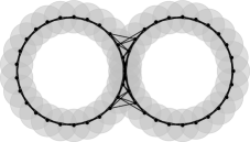
As far as we know, Bendich and Harer Bendich11 , while discussing other dependencies of persistent intersection homology, did not discuss this aspect. Yet, it is crucial to get persistent intersection homology to “detect” those singularities if we want to understand the manifold structure of a given data set. To circumvent this issue, we propose obtaining additional information about the geometry of a given point cloud in order to determine which points are supposed to be singular. Alternatively, we could try to learn a suitable stratification of the whole space Bendich12 at the cost of reduced performance.

3.1 Choosing a Stratification

Having seen that the utility and expressiveness of persistent intersection homology hinge upon the choice of a stratification, we now develop several constructions. We restrict ourselves to the detection of isolated singular points, i.e., vertices or $0$-simplices, in this paper. A stratification should ideally reflect the existence of singularities in a data set. For the example shown in Figure 3, a singularity exists at $A$ because the “whisker” will remain a one-dimensional piece regardless of the scale at which we look at the data, while the triangle is a two-dimensional object. This observation leads to a set of stratification strategies, which we first detail before applying them in Section 4.

Dimensionality-Based Stratifications

In order to stratify unstructured data according to the local intrinsic dimensionality, we propose the following scheme. We first obtain the $k$ nearest neighbors of every data point and treat them as local patches. For each of these subsets, we perform a principal component analysis (PCA) and obtain the respective set of eigenvalues $\{\lambda_{1},\dots,\lambda_{d}\}$, where $d$ refers to the maximum number of attributes in the point cloud. We then calculate the largest spectral gap, i.e.,

$$d_{i}:=\operatorname*{arg\,max}_{j\in\{2,\dots,d\}}|\lambda_{j}-\lambda_{j-1}|-1,$$ (8)

and use it as an estimate of the local intrinsic dimensionality at the $i$^th data point. Points that can be well represented by a single eigenvalue are thus taken to correspond to a locally one-dimensional patch in the data, for example. In practice, as PCA is not robust against outliers, one typically requires some smoothing iterations for the estimates. We use several iterations of smoothing based on nearest neighbors, similar to mean shift clustering Cheng95 . The resulting values can then be used to stratify according to local dimensionality.

Density-based Stratifications

We can also stratify unstructured data according to the behavior of a density estimator, such as a truncated Gaussian kernel, i.e.,

$$f(x):={\sum}_{y\neq x}\exp{\bigg{(}-\frac{\operatorname{dist}^{2}(x,y)}{2h}\bigg{)}},$$ (9)

where $h$ is the bandwidth of the estimator and we define the exponential expression to be $0$ if $\operatorname{dist}(x,y)>h$. The density values give rise to a distribution of values so that we can use standard outlier detection methods. Once outliers have been identified, they can be put into the first subset of the filtration. This approach has the advantage of rapidly detecting interesting data points but it cannot be readily extended to higher-dimensional simplices.

Curvature-Based Stratifications

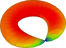
The curvature of a manifold is an important property that can be used to detect differences in local structure. Using a standard algorithm to estimate curvature in meshes Meyer03 , we can easily identify a region around the singular point in the “pinched torus” as having an extremely small curvature. Figure LABEL:fig:Pinched_torus_curvature depicts this. For higher-dimensional point clouds, we propose obtaining an approximation of curvature by using the curvature of high-dimensional spheres that are fit to local patches of a point cloud. More precisely, we extract the $k$ nearest neighbors of every point in a point cloud and fit a high-dimensional sphere. Such a fit can be accomplished using standard least squares approaches, such as the one introduced by Pratt Pratt87 .

4 Results

In the following, we discuss the benefits of persistent intersection homology over ordinary persistent homology by means of several data sets, containing random samples of non-trivial topological pseudomanifolds, as well as experimental data from image processing.

4.1 Wedge of Spheres

(a) Density

(b) Local dimension (smoothed)

Figure 5: A random sample of $S^{2}\vee S^{2}$, color-coded by two stratification strategies. Both descriptors register either extremely high (density) or extremely low (dimensionality) values as we approach the singular part of the data set. The corresponding points are put into $X_{0}$.

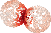
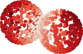
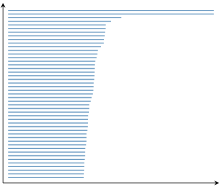
We extend the example depicted in Figure 4 and sample points at random from a wedge of $2$-spheres. If no precautions are taken, the resulting data set suffers from the problem that we previously outlined. We thus use it to demonstrate the efficacy of our stratification strategies. Figure 5 depicts the data set along with two different descriptors. In both cases, we build a simple stratification in which $X_{0}$ contains all singular points, $X_{1}=X_{0}$, and $X_{2}=\mathrm{K}$, i.e., the original space. We use the default Goresky–MacPherson perversity $\bar{p}^{\prime}=(0)$. This suffices to detect that the data set is not a manifold: we obtain $\beta_{0}=2$ for both stratification strategies, whereas persistent homology only shows $\beta_{0}=1$. Figure 6 depicts excerpts of the zero-dimensional barcodes for the data set. The two topological features with infinite persistence are clearly visible in the persistent intersection homology barcode. Since $\beta_{2}=2$, this re-establishes Poincaré duality.

(a) Persistent homology

(b) Persistent intersection homology

Figure 6: Excerpt of the zero-dimensional barcodes for $S^{2}\vee S^{2}$. With persistent homology LABEL:sub@sfig:S2vS2_barcode_PH, no additional connected component appears, whereas with persistent intersection homology LABEL:sub@sfig:S2vS2_barcode_IH with the density-based stratification, the singular point/region results in splitting the data.

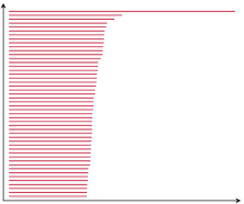
4.2 Pinched Torus

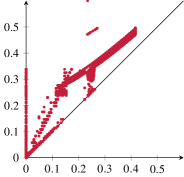
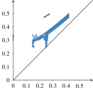
We demonstrate the curvature-based stratification using the “pinched torus” data set. Figure LABEL:fig:Pinched_torus_curvature depicts the torus along with curvature estimates. A standard outlier test helps us detect the region around the singular point. We set up the stratification such that $X_{0}$ contains all points from the detected region, $X_{1}=X_{0}$, and $X_{2}=\mathrm{K}$. Moreover, we use $\bar{p}^{\prime}=(0)$ because the dimensionality of the input data prevents us from detecting any higher-dimensional features. Persistent homology shows that the point cloud contains a persistent cycle in dimension one. Essentially, the data are considered to be a “thickened circle”. Figure 7 depicts the persistence diagrams. We can see that the point with infinite persistence (shown in Figure 7a at the top border) is missing in addition to many other points in the persistent intersection homology diagram (Figure 7b). The Wasserstein distance Edelsbrunner10 between the two diagrams is thus large, indicating the non-manifold structure of the data.

(a) Persistent homology

(b) Persistent intersection homology

Figure 7: Persistent homology detects more one-dimensional features for the “pinched torus” data set than persistent intersection homology.

4.3 Synthetic Faces

This data set was originally used to demonstrate the effectiveness of nonlinear dimensionality reduction algorithms Tenenbaum00 . Previous research demonstrated that the data set does not exhibit uniform density Rieck15b , which makes the existence of (isolated) singular points possible. It is known that the intrinsic dimension of the data set is three, so we shall only take a look at low-dimensional topological features. More precisely, using the curvature-based stratification, we want to see how persistence diagrams in dimensions 0–2 change when we calculate intersection homology. Note that analyzing three-dimensional features is not expedient, because the stratification cannot detect deviations from “manifoldness” in this dimension.

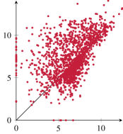
Figure 8 depicts the zero-dimensional barcodes of the data set. They are virtually identical for both methods (we find that their Wasserstein distance is extremely small), except for some minor shifts in the destruction values, i.e., the endpoints of every interval. This indicates that the singular points only have a very local influence on the structure of the data set; they are not resulting in a split, for example. For dimensions one and two, depicted by Figure 9, we observe a similar behavior. The overall structure of both persistence diagrams is similar, and there is only a slight decrease in total persistence Cohen-Steiner10 for persistent intersection homology. Likewise, the Wasserstein distance between both diagrams is extremely small.

In summary, we see that we are unable to detect significant differences in zero-dimensional, one-dimensional, and two-dimensional topological features. This lends credibility to the assumption that the data set is a single manifold.

(a) Persistent homology

(b) Persistent intersection homology

Figure 8: Zero-dimensional barcodes for the “Synthetic Faces” data set. Both barcodes are virtually identical, indicating that the singular points do not influence connected components.

(a) Persistent homology

(b) Persistent intersection homology

Figure 9: Comparison of persistent homology in dimension one (above diagonal) and two (below diagonal) for the “Synthetic Faces” data set. The overall structure is similar, and only few features disappear during the calculation of persistent intersection homology.

5 Conclusion

We showed how to use persistent intersection homology for the analysis of data sets that might not represent a single manifold. Moreover, we described some pitfalls when applying this technique—namely, finding suitable stratifications, and presented several strategies for doing so. We demonstrated the utility of persistent intersection homology on several data sets of low intrinsic dimensionality. Future work could focus on improving the performance of the admissibility condition in Eq. 7 to process data sets with higher intrinsic dimensions. It would also be interesting to extend stratification strategies to higher-dimensional strata, i.e., singular regions instead of singular points.

References

- (1) Bendich, P.: Analyzing stratified spaces using persistent versions of intersection and local homology. Ph.D. thesis, Duke University (2009)
- (2) Bendich, P., Harer, J.: Persistent intersection homology. FoCM 11(3), 305–336 (2011)
- (3) Bendich, P., Wang, B., Mukherjee, S.: Local homology transfer and stratification learning. In: Y. Rabani (ed.) Symposium on Discrete Algorithms, pp. 1355–1370. SIAM (2012)
- (4) Carlsson, G.: Topological pattern recognition for point cloud data. Acta Numerica 23, 289–368 (2014)
- (5) Cheng, Y.: Mean shift, mode seeking, and clustering. IEEE TPAMI 17(8), 790–799 (1995)
- (6) Cohen-Steiner, D., Edelsbrunner, H., Harer, J.: Stability of persistence diagrams. Discrete & Computational Geometry 37(1), 103–120 (2007)
- (7) Cohen-Steiner, D., Edelsbrunner, H., Harer, J.: Extending persistence using Poincaré and Lefschetz duality. FoCM 9(1), 79–103 (2009)
- (8) Cohen-Steiner, D., Edelsbrunner, H., Harer, J., Mileyko, Y.: Lipschitz functions have -stable persistence. Foundations of Computational Mathematics 10(2), 127–139 (2010)
- (9) Donoho, D.L., Grimes, C.: Image manifolds which are isometric to Euclidean space. Journal of Mathematical Imaging and Vision 23(1), 5–24 (2005)
- (10) Edelsbrunner, H., Harer, J.: Computational topology: An introduction. AMS (2010)
- (11) Edelsbrunner, H., Morozov, D.: Persistent homology: Theory and practice. In: European Congress of Mathematics. EMS Publishing House, Zürich, Switzerland (2014)
- (12) Fefferman, C., Mitter, S., Narayanan, H.: Testing the manifold hypothesis. Journal of the American Mathematical Society 29(4), 983–1049 (2016)
- (13) Goresky, M., MacPherson, R.: Intersection homology theory. Topology 19(2), 135–162 (1980)
- (14) Hinton, G.E., Dayan, P., Revow, M.: Modeling the manifolds of images of handwritten digits. IEEE Transactions on Neural Networks 8(1), 65–74 (1997)
- (15) Kirwan, F., Woolf, J.: An Introduction to Intersection Homology Theory, 2nd edn. Chapman and Hall/CRC, Boca Raton, FL, USA (2006)
- (16) MacPherson, R., Vilonen, K.: Elementary construction of perverse sheaves. Inventiones mathematicae 84(2), 403–435 (1986)
- (17) Meyer, M., Desbrun, M., Schröder, P., Barr, A.H.: Discrete differential-geometry operators for triangulated -manifolds. In: H.C. Hege, K. Polthier (eds.) Visualization and Mathematics III, pp. 35–57. Springer, Heidelberg (2003)
- (18) Narayanan, H., Mitter, S.: Sample complexity of testing the manifold hypothesis. In: NIPS 23, pp. 1786–1794. Curran Associates, Inc., Red Hook, NY, USA (2010)
- (19) Pratt, V.: Direct least-squares fitting of algebraic surfaces. ACM SIGGRAPH Computer Graphics 21(4), 145–152 (1987)
- (20) Rieck, B., Leitte, H.: Persistent homology for the evaluation of dimensionality reduction schemes. Computer Graphics Forum 34(3), 431–440 (2015)
- (21) Roweis, S.T., Saul, L.K.: Nonlinear dimensionality reduction by locally linear embedding. Science 290(5500), 2323–2326 (2000)
- (22) Saul, L.K., Roweis, S.T.: Think globally, fit locally: Unsupervised learning of low dimensional manifolds. Journal of Machine Learning Research 4, 119–155 (2003)
- (23) de Silva, V., Morozov, D., Vejdemo-Johansson, M.: Dualities in persistent (co)homology. Inverse Problems 27(12), 124,003 (2011)
- (24) Singh, G., Mémoli, F., Carlsson, G.: Topological methods for the analysis of high dimensional data sets and 3D object recognition. In: Eurographics Symposium on Point-Based Graphics. Eurographics Association (2007)
- (25) Tenenbaum, J.B., de Silva, V., Langford, J.C.: A global geometric framework for nonlinear dimensionality reduction. Science 290(5500), 2319–2323 (2000)