Improved randomized algorithm for $k$-submodular function maximization

Abstract

Submodularity is one of the most important properties in combinatorial optimization, and $k$-submodularity is a generalization of submodularity. Maximization of a $k$-submodular function requires an exponential number of value oracle queries, and approximation algorithms have been studied. For unconstrained $k$-submodular maximization, Iwata et al. gave randomized $k/(2k-1)$-approximation algorithm for monotone functions, and randomized $1/2$-approximation algorithm for nonmonotone functions.

In this paper, we present improved randomized algorithms for nonmonotone functions. Our algorithm gives $\frac{k^{2}+1}{2k^{2}+1}$-approximation for $k\geq 3$. We also give a randomized $\frac{\sqrt{17}-3}{2}$-approximation algorithm for $k=3$. We use the same framework used in Iwata et al. and Ward and Živný with different probabilities.

90C27

1 Introduction

A set function $f:2^{V}\to\mathbb{R}$ is submodular if, for any $A,B\subseteq V$, $f(A)+f(B)\geq f(A\cup B)+f(A\cap B)$. Submodularity is one of the most important properties of combinatorial optimization. The rank functions of matroids and cut capacity functions of networks are submodular. Submodular functions can be seen as a discrete version of convex functions [4, 5, 12].

For submodular function minimization, Grötschel et al. [7] showed the first polynomial-time algorithm. The combinatorial strongly polynomial algorithms were shown by Iwata et al. [9] and Schrijver [14]. On the other hand, submodular function maximization requires an exponential number of value oracle queries, and we are interested in designing approximation algorithms. Let $f$ be an input function for maximization, $S^{*}$ be a maximizer of $f$, and $S$ be the output of an algorithm. The approximation ratio of the algorithm is defined as $f(S)/f(S^{*})$ for deterministic algorithms and $\mathbb{E}[f(S)]/f(S^{*})$ for randomized algorithms. For unconstrained submodular maximization, the randomized algorithm [2] achieves $1/2$-approximation. Feige et al. [3] showed $(1/2+\epsilon)$-approximation requires an exponential number of value oracle queries. This implies that, the algorithm is one of the best algorithms in terms of the approximation ratio. Buchbinder and Feldman [1] showed a derandomized version of the randomized algorithm [2], and it achieves $1/2$-approximation.

$k$-submodularity is an extension of submodularity. It was first introduced by Huber and Kolmogolov [8]. A $k$-submodular function is defined as follows. Note that $[k]=\{1,2,\ldots,k\}$.

Definition 1.1.

([8]) Let $(k+1)^{V}:=\{(X_{1},...,X_{k})\mid X_{i}\subseteq V\ (i\in[k]),X_{i}\cap X_{j}=\emptyset\ (i\neq j)\}$. A function $f:(k+1)^{V}\to\mathbb{R}$ is called $k$-submodular if we have

$$f(\boldsymbol{x})+f(\boldsymbol{y})\geq f(\boldsymbol{x}\sqcap\boldsymbol{y})+f(\boldsymbol{x}\sqcup\boldsymbol{y})$$

for any $\boldsymbol{x}=(X_{1},...,X_{k}),\ \boldsymbol{y}=(Y_{1},...,Y_{k})\in(k+1)^{V}$, where

$$\boldsymbol{x}\sqcap\boldsymbol{y} = (X_{1}\cap Y_{1},...,X_{k}\cap Y_{k})\ \ and$$

$$\boldsymbol{x}\sqcup\boldsymbol{y} = (X_{1}\cup Y_{1}\backslash\bigcup_{i\neq 1}(X_{i}\cup Y_{i}),...,X_{k}\cup Y_{k}\backslash\bigcup_{i\neq k}(X_{i}\cup Y_{i})).$$

It is a submodular function if $k=1$. It is called a bisubmodular function if $k=2$. We can see applications of $k$-submodular functions in influence maximization and sensor placement [13] and computer vision [6].

Maximization for $k$-submodular functions also requires an exponential number of value oracle queries, and approximation algorithms have been studied. Input of the problem is a nonnegative $k$-submodular function. Note that, for any $k$-submodular function $f$ and any $c\in\mathbb{R}$, a function $f^{\prime}(\boldsymbol{x}):=f(\boldsymbol{x})+c$ is $k$-submodular. Output of the problem is $\boldsymbol{x}=(X_{1},...,X_{k})\in(k+1)^{V}$. The input function is accessed via value oracle queries. For bisubmodular functions, Iwata et al. [10] and Ward and Živný [15] showed that the algorithm for submodular functions [2] can be extended. Ward and Živný [15] analyzed an extension for $k$-submodular functions. They showed a randomized $1/(1+a)$-approximation algorithm with $a=\max\{1,\sqrt{(k-1)/4}\}$ and a deterministic $1/3$-approximation algorithm. Later Iwata et al. [11] showed a randomized $1/2$-approximation algorithm. For monotone $k$-submodular functions, they also gave a randomized $\frac{k}{2k-1}$-approximation algorithm. They also showed any $(\frac{k+1}{2k}+\epsilon)$-approximation algorithm requires an exponential number of value oracle queries.

In this paper, we improve randomized algorithms for nonmonotone functions. Our algorithm gives $\frac{k^{2}+1}{2k^{2}+1}$-approximation for $k\geq 3$. We also give randomized $\frac{\sqrt{17}-3}{2}$-approximation algorithm for $k=3$. We use the same framework used in [11] and [15] with different probabilities.

The rest of this paper is organized as follows. In Section 2, we explain details of $k$-submodularity. We also explain previous works of unconstrained $k$-submodular maximization. In Section 3, we give $\frac{\sqrt{17}-3}{2}$-approximation algorithm for $k=3$. In Section 4, we give $\frac{k^{2}+1}{2k^{2}+1}$-approximation algorithm for $k\geq 3$. We conclude this paper in Section 5.

2 Preliminary and previous works

Define a partial order $\preceq$ on $(k+1)^{V}$ for $\boldsymbol{x}=(X_{1},...,X_{k})$ and $\boldsymbol{y}=(Y_{1},...,Y_{k})$ as follows:

$$\boldsymbol{x}\preceq\boldsymbol{y}\overset{\mathrm{def}}{\Longleftrightarrow}X_{i}\subseteq Y_{i}\ (i\in[k]).$$

A monotone $k$-submodular function is $k$-submodular and satisfies $f(\boldsymbol{x})\leq f(\boldsymbol{y})$ for any $\boldsymbol{x}=(X_{1},...,X_{k})$ and $\boldsymbol{y}=(Y_{1},...,Y_{k})$ in $(k+1)^{V}$ with $\boldsymbol{x}\preceq\boldsymbol{y}$.

The property of $k$-submodularity can be written as another form. For $\boldsymbol{x}=(X_{1},...,X_{k})\in(k+1)^{V}$, $e\notin\bigcup_{l=1}^{k}X_{l}$, and $i\in[k]$, define

$$\Delta_{e,i}f(\boldsymbol{x})=f(X_{1},...,X_{i-1},X_{i}\cup\{e\},X_{i+1},...,X_{k})-f(X_{1},...,X_{k}).$$

Theorem 2.1.

([15] Theorem 7) A function $f:(k+1)^{V}\to\mathbb{R}$ is $k$-submodular if and only if $f$ is orthant submodular and pairwise monotone, where $f$ is orthant submodular if

$$\Delta_{e,i}f(\boldsymbol{x})\geq\Delta_{e,i}f(\boldsymbol{y})\ (\boldsymbol{x},\boldsymbol{y}\in(k+1)^{V},\ \boldsymbol{x}\preceq\boldsymbol{y},\ e\notin\bigcup_{l=1}^{k}Y_{l},\ i\in[k]),$$

and pairwise monotone if

$$\Delta_{e,i}f(\boldsymbol{x})+\Delta_{e,j}f(\boldsymbol{x})\geq 0\ (\boldsymbol{x}\in(k+1)^{V},\ e\notin\bigcup_{l=1}^{k}X_{l},\ i,j\in[k]\ (i\neq j)).$$

To analyze $k$-submodular functions, it is often convenient to identify $(k+1)^{V}$ with $\{0,1,...,k\}^{V}$. Let $n=|V|$. An $n$-dimensional vector $\boldsymbol{x}\in\{0,1,...,k\}^{V}$ is associated with $(X_{1},...,X_{k})\in(k+1)^{V}$ by $X_{i}=\{e\in V\mid\boldsymbol{x}(e)=i\}$.

2.1 Algorithm framework

In this section, we introduce the algorithm framework discussed in [10, 11, 15]. Iwata et al. [10] and Ward and Živný [15] used it with specific probability distributions.

Algorithm 1 ([11] Algorithm 1)

1: Input: A nonnegative $k$-submodular function $f:\{0,1,...,k\}^{V}\to\mathbb{R}_{+}$.

2: Output: A vector $\boldsymbol{s}\in\{0,1,...,k\}^{V}$.

3:$\boldsymbol{s}\leftarrow\boldsymbol{0}\$.

4:Denote the elements of $V$ by $e^{(1)},...,e^{(n)}\ (|V|=n)$.

5:for $t=1,...,n$ do

6:     Set a probability distribution $\{p_{i}\}$ over $[k]$.

7:     Let $\boldsymbol{s}(e^{(t)})\in[k]$ be chosen randomly with $\mathrm{Pr}[\boldsymbol{s}(e^{(t)})=i]=p_{i}^{(t)}$.

8:end for

9:return $\boldsymbol{s}$

Now we define some variables to see Algorithm 1. Let $\boldsymbol{o}$ be an optimal solution. We consider the $t$-th iteration of the algorithm, and we write $\boldsymbol{s}^{(t)}$ as the solution $\boldsymbol{s}$ after the $t$-th iteration. Let other variables be as follows:

$$\boldsymbol{o}^{(t)} = (\boldsymbol{o}\sqcup\boldsymbol{s}^{(t)})\sqcup\boldsymbol{s}^{(t)},$$

$$\boldsymbol{t}^{(t-1)}(e) = \begin{cases}\boldsymbol{o}^{(t)}(e)&(e\neq e^{(t)})\\ 0&(e=e^{(t)})\end{cases},$$

$$y_{i}^{(t)} = \Delta_{e^{(t)},i}f(\boldsymbol{s}^{(t-1)}),\ a_{i}^{(t)}=\Delta_{e^{(t)},i}f(\boldsymbol{t}^{(t-1)}).$$

From the updating rule in the algorithm, $\boldsymbol{o}^{(t)}(e)=\boldsymbol{s}(e)$ for $e\in\{e^{(1)},...,e^{(t)}\}$, and $\boldsymbol{o}^{(t)}(e)=\boldsymbol{o}(e)$ for $e\in\{e^{(t+1)},...,e^{(n)}\}$. Algorithm 1 satisfies the following lemma.

Lemma 2.2.

([11] Lemma 2.1.)
Let $c\in\mathbb{R}_{+}$. Conditioning on $\boldsymbol{s}^{(t-1)}$, suppose that

(1) $$\sum_{i=1}^{k}(a_{i^{*}}^{(t)}-a_{i}^{(t)})p_{i}^{(t)}\leq c\sum_{i=1}^{k}(y_{i}^{(t)}p_{i}^{(t)})$$

holds for each $t$ with $1\leq t\leq n$, where $i^{*}=\boldsymbol{o}(e^{(t)})$. Then $\mathbb{E}[f(\boldsymbol{s})]\geq\frac{1}{1+c}f(\boldsymbol{o})$.

In the rest of this paper, we write $y_{i}^{(t)},\ a_{i}^{(t)}$ as $y_{i},\ a_{i}$ for the simplicity if it is clear from the context.

Our goal is to set up $\{p_{i}\}$ such that (1) holds as large $c$ as possible. Although $\{a_{i}\}$ and $\{y_{i}\}$ are uncontrollable, we know that those satisfy (2), (3), and (4) by orthant submodurality and pairwise monotonicity.

(2) $$a_{i} \leq y_{i}\ (i\in[k])$$

(3) $$a_{i}+a_{j} \geq 0\ (i,j\in[k],\ i\neq j)$$

(4) $$y_{i}+y_{j} \geq 0\ (i,j\in[k],\ i\neq j).$$

Hence in order to get $\frac{1}{1+c}$-approximation, it is sufficient to give probability distribution $\{p_{i}\}$ that satisfies 1, for any $a_{1},...,a_{k},y_{1},...,y_{k}$ with (2), (3), and (4).

2.2 The randomized algorithm for monotone functions

Our algorithm for nonmonotone $k$-submodular functions also uses an idea developed for maximizing monotone $k$-submodular functions in [11]. The following is the randomized algorithm for maximizing monotone $k$-submodular functions in [11].

Algorithm 2 ([11] Algorithm 3)

1: Input: A monotone $k$-submodular function $f:\{0,1,...,k\}^{V}\to\mathbb{R}_{+}$.

2: Output: A vector $\boldsymbol{s}\in\{0,1,...,k\}^{V}$.

3:$\boldsymbol{s}\leftarrow\boldsymbol{0}$, $\alpha\leftarrow k-1$.

4:Denote the elements of $V$ by $e^{(1)},...,e^{(n)}\ (|V|=n)$.

5:for $t=1,...,n$ do

6:     $y_{i}^{(t)}\leftarrow\Delta_{e^{(t)},i}f(\boldsymbol{s})\ \ (i\in[k])$.

7:     $\beta\leftarrow\sum^{k}_{i=1}(y_{i}^{(t)})^{\alpha}$.

8:     if $\beta\neq 0$ then  $p_{i}^{(t)}\leftarrow(y_{i}^{(t)})^{\alpha}/\beta\ \ (i\in[k])$.

9:     else

10:         $p_{1}^{(t)}=1,p_{i}^{(t)}=0\ (i\in\{2,...,k\})$.

11:     end if

12:     Let $\boldsymbol{s}(e^{(t)})\in[k]$ be chosen randomly with $\mathrm{Pr}[\boldsymbol{s}(e^{(t)})=i]=p_{i}^{(t)}$.

13:end for

14:return $\boldsymbol{s}$

Note that this algorithm follows the framework Algorithm 1. For the analysis, the next lemma is proved in [11].

Lemma 2.3.

([11], proof of Theorem 2.2.) Let $k$ be a positive integer, $y_{i}(i=1,...,k)$ be nonnegative, and $i^{*}\in[k]$.

(5) $$\left(1-\frac{1}{k}\right)\sum_{i=1}^{k}p_{i}y_{i}\geq\sum_{i\neq i^{*}}p_{i}y_{i^{*}}$$

is always satisfied by the probability distribution $\{p_{i}\}$ in Algorithm 2.

For monotone $k$-submodular function, $a_{1},...,a_{k}$, $y_{1},...,y_{k}$ also satisfy

(6) $$y_{i}\geq 0,a_{i}\geq 0\ (i\in[k]).$$

From Lemma 2.3, (2), and (6), (1) follows for $c=1-\frac{1}{k}$ and $p_{1},...,p_{k}$ given in Algorithm 2. The approximation ratio of Algorithm 2 is $\frac{k}{2k-1}$, following from Lemma 2.2, Lemma 2.3, (2), and (6) [11].

3 A randomized algorithm for $k=3$

In this section, we give an improved algorithm for $k$-submodular maximization with $k=3$. We use the framework of randomized algorithms (Algorithm 1) with a different probability distribution.

3.1 An improved analysis of Algorithm 1

As reviewed in Section 2.1, Lemma 2.2 plays a key role in the analysis of an approximation algorithm based on the framework Algorithm 1. In this section, we first show that Lemma 2.2 can be improved. From pairwise monotonicity, we have $a_{i}+a_{j}\geq 0\ (i\neq j)$. Therefore, the number of $i$ with $a_{i}<0$ is at most one.

Lemma 3.1.

Let $c\in\mathbb{R}_{+}$, and $i^{*}=\boldsymbol{o}(e^{(t)})$. If there is an index $i$ with $a_{i}<0$, we call it $i_{-}$. Suppose that the following inequalities hold for each $t$ with $1\leq t\leq n$. Then $\mathbb{E}[f(\boldsymbol{s})]\geq\frac{1}{1+c}f(\boldsymbol{o})$.

(7) $$c\sum_{i=1}^{k}(y_{i}p_{i})\geq\begin{cases}0&(\text{if}\ a_{i_{-}}<0\ \text{and}\ i_{-}=i^{*})\\ (1-p_{i^{*}})a_{i^{*}}+(1-p_{i^{*}}-2p_{i_{-}})a_{i_{-}}&(\text{if}\ a_{i_{-}}<0\ \text{and}\ i_{-}\neq i^{*})\\ (1-p_{i^{*}})a_{i^{*}}&(\text{if}\ a_{i}\geq 0\ \text{for any}\ i)\\ \end{cases}$$

Proof 3.2.

By Lemma 2.2, it suffices to show

(8) $$\sum_{i=1}^{k}(a_{i^{*}}-a_{i})p_{i}$$

$$\leq \begin{cases}0&(\text{if}\ a_{i_{-}}<0\ \text{and}\ i_{-}=i^{*})\\ (1-p_{i^{*}})a_{i^{*}}+(1-p_{i^{*}}-2p_{i_{-}})a_{i_{-}}&(\text{if}\ a_{i_{-}}<0\ \text{and}\ i_{-}\neq i^{*})\\ (1-p_{i^{*}})a_{i^{*}}&(\text{if}\ a_{i}\geq 0\ \text{for any}\ i)\end{cases}.$$

From the definition, $p_{1},...,p_{k}$ follows $p_{i}\geq 0$ for any $i$ and $\sum_{i=1}^{k}p_{i}=1$.

Suppose $a_{i}\geq 0$ for any $i$. From

$$\sum_{i=1}^{k}(a_{i^{*}}-a_{i})p_{i}\leq\sum_{i\neq i^{*}}a_{i^{*}}p_{i}=(1-p_{i^{*}})a_{i^{*}},$$

we obtain (8).

Thus suppose $a_{i_{-}}<0$. If $i_{-}\neq i^{*}$, from pairwise monotonicity, we have $a_{i_{-}}\geq-a_{i}(i\neq i_{-})$. Hence

$$\sum_{i=1}^{k}(a_{i^{*}}-a_{i})p_{i} \leq (a_{i^{*}}-a_{i_{-}})p_{i_{-}}+\sum_{i\neq i^{*},i_{-}}(a_{i^{*}}+a_{i_{-}})p_{i}$$

$$= (1-p_{i^{*}})a_{i^{*}}+(1-p_{i^{*}}-2p_{i_{-}})a_{i_{-}}.$$

holds. Therefore, we obtain (8).

Finally, suppose $i_{-}=i^{*}$. In this case, we have $a_{i^{*}}<0$ and $a_{i}\geq|a_{i^{*}}|>0$ for $i\neq i^{*}$ from the pairwise monotonicity. Therefore we can see $(a_{i^{*}}-a_{i})p_{i}\leq 0$ for any $i$.

From Lemma 3.1, to show the approximation ratio, it is sufficient to give $c$, $p_{1},...,p_{k}$ which follows

$$c>0,\ p_{1},...,p_{k}\geq 0,\ \sum_{i=1}^{k}p_{i}=1$$

for any $a_{1},...,a_{k}$, $y_{1},...,y_{k}$, $i^{*},i_{-}$ which satisfies (2), (3), (4), $i^{*}\neq i_{-}$, and

$$a_{i_{-}}<0\ ({\rm if\ there\ is\ negative\ }a_{i}).$$

Note that we can only use the information of $y_{1},...,y_{k}$ to give $c$, $p_{1},...,p_{k}$.

Motivated by Lemma 3.1, for given $a_{1},...,a_{k}$, $y_{1},...,y_{k}$ in $\mathbb{R}$, and $i^{*},i_{-}$ in $\{1,...,k\}$ with $i^{*}\neq i_{-}$, we define $f,g:\mathbb{R}^{k}\to\mathbb{R}$ by

(9) $$\begin{cases}f(\boldsymbol{p}):=\begin{cases}0&(\text{if}\ a_{i_{-}}<0\ \text{and}\ i^{*}=i_{-})\\ (1-p_{i^{*}})a_{i^{*}}+(1-p_{i^{*}}-2p_{i_{-}})a_{i_{-}}&(\text{if}\ a_{i_{-}}<0\ \text{and}\ i^{*}\neq i_{-})\\ (1-p_{i^{*}})a_{i^{*}}&(\text{if}\ a_{i}\geq 0\ \text{for any}\ i)\end{cases},\\ g(\boldsymbol{p}):=\sum_{i=1}^{k}(y_{i}p_{i}).\end{cases}$$

Then (7) can be written as $f(\boldsymbol{p})\leq cg(\boldsymbol{p})$．

3.2 The improved algorithm for the case $k=3$

In this section, we show the $\frac{\sqrt{17}-3}{2}$-approximation algorithm for the case $k=3$. In view of Lemma 3.1, our goal is to set up $p_{1},p_{2},p_{3}$ that satisfy (8) with $c=\frac{\sqrt{17}-1}{4}$. We show that the following implementation of Algorithm 1 achieves this goal.

Algorithm 3 A randomized $3$-submodular functions maximization algorithm

1:$\boldsymbol{s}\leftarrow\boldsymbol{0}\ (\boldsymbol{s}\in\{0,1,2,3\}^{V})$.

2:for $t=1,...,n$ do

3:     $y_{i}\leftarrow\Delta_{e,i}f(\boldsymbol{s})\ (i\in[k])$.

4:     Assume $y_{1}\geq y_{2}\geq y_{3}$.

5:     $\beta\leftarrow\frac{y_{2}}{y_{1}},\ \gamma=\frac{y_{3}}{y_{1}}.$

6:     $\delta\leftarrow\frac{1-\beta-\gamma}{2}+\frac{\beta}{1+\gamma}-\frac{\gamma}{\beta+\gamma}.$

7:     if $\gamma\leq 0$ then $p_{1}^{(t)}\leftarrow\frac{1}{1+\beta},\ p_{2}^{(t)}\leftarrow\frac{\beta}{1+\beta},\ p_{3}^{(t)}\leftarrow 0.$

8:     else if $\delta>0$ then $p_{1}^{(t)}\leftarrow\frac{1+\gamma}{1+\beta+2\gamma},\ p_{2}^{(t)}\leftarrow\frac{\beta+\gamma}{1+\beta+2\gamma},\ p_{3}^{(t)}\leftarrow 0.$

9:     else

10:         $p_{1}^{(t)}\leftarrow\frac{2-\beta+\gamma}{2+\beta+3\gamma},\ p_{i}^{(t)}\leftarrow\frac{\beta+\gamma}{2+\beta+3\gamma}\ (i\neq 1).$

11:     end if

12:     Let $\boldsymbol{s}(e^{(t)})\in[3]$ be chosen randomly with $\mathrm{Pr}[\boldsymbol{s}(e^{(t)})=i]=p_{i}^{(t)}$.

13:end for

14:return $\boldsymbol{s}$

The probability distribution in Algorithm 3 is motivated by the next lemma.

Lemma 3.3.

Let $y_{1},y_{2},y_{3},a_{1},a_{2},a_{3}$ as any number satisfy (2), (3), (4) and $y_{1}\geq y_{2}\geq y_{3}$. 　Let $i_{-}$ be the index $i$ with $a_{i}<0$ if it exists, and let $i^{*}$ be any number in $\{1,2,3\}$.

Define $p_{1},p_{2},p_{3}$ by

(10) $$\begin{cases}p_{1}=\frac{1}{1+\beta},p_{2}=\frac{\beta}{1+\beta},p_{3}=0&(\text{if}\ \gamma\leq 0)\\ p_{1}=\frac{1+\gamma}{1+\beta+2\gamma},p_{2}=\frac{\beta+\gamma}{1+\beta+2\gamma},p_{3}=0&(\text{if}\ \gamma>0,\delta>0)\\ p_{1}=\frac{2-\beta+\gamma}{2+\beta+3\gamma},p_{2}=p_{3}=\frac{\beta+\gamma}{2+\beta+3\gamma}&(\text{if}\ \gamma>0,\delta\leq 0)\end{cases}$$

where

(11) $$\beta=\frac{y_{2}}{y_{1}},\gamma=\frac{y_{3}}{y_{1}},\delta=\frac{1-\beta-\gamma}{2}+\frac{\beta}{1+\gamma}-\frac{\gamma}{\beta+\gamma}.$$

Then the inequality (7) holds with $c=\frac{\sqrt{17}-1}{4}$.

Proof 3.4.

Note that $p_{1}\geq p_{2}\geq p_{3}$. From $p_{1}\geq p_{2}\geq p_{3}\geq 0$, $y_{1}\geq y_{2}\geq y_{3}$, and (4), we obtain

$$g(\boldsymbol{p})\geq p_{3}(y_{1}+y_{2}+y_{3})\geq 0.$$

Therefore, $f(\boldsymbol{p})\leq cg(\boldsymbol{p})$ holds for $a_{i_{-}}<0$ and $i_{-}=i^{*}$. If $f(\boldsymbol{p})\leq 0$, we also have $f(\boldsymbol{p})\leq cg(\boldsymbol{p})$. Now suppose $f(\boldsymbol{p})>0$ and $i_{-}=i^{*}$ if $a_{i_{-}}<0$.

It is convenient to have a list of the values of $1-p_{i^{*}}-2p_{i_{-}}$ and $f(\boldsymbol{p})$, for each case of $i^{*}$ and $i_{-}$ on Table 1. For the inequalities in the column of $1-p_{i^{*}}-2p_{i_{-}}$, we used $p_{1}\geq p_{2}\geq p_{3}$ which follows from the definition (10). For the inequalities in the column of $f(\boldsymbol{p})$, we used $y_{i}\geq a_{i}(i\in[k])$ and $a_{i}+a_{j}\geq 0$, which follows from the definition (2) and (3).

Table 1: Upper bound of $f(\boldsymbol{p})$.

$i^{*}$	$i_{-}$	$1-p_{i^{*}}-2p_{i_{-}}$	$f(\boldsymbol{p})$
$1$	$2$	$1-p_{1}-2p_{2}=p_{3}-p_{2}\leq 0$	$(p_{2}+p_{3})a_{1}+(p_{3}-p_{2})a_{2}$	$\leq$	$(p_{2}+p_{3})y_{1}+(p_{2}-p_{3})y_{3}$
$1$	$3$	$1-p_{1}-2p_{3}=p_{2}-p_{3}\geq 0$	$(p_{2}+p_{3})a_{1}$	$\leq$	$(p_{2}+p_{3})y_{1}$
$2$	$1$	$1-p_{2}-2p_{1}=p_{3}-p_{1}\leq 0$	$(p_{1}+p_{3})a_{2}+(p_{3}-p_{1})a_{1}$	$\leq$	$(p_{1}+p_{3})y_{2}+(p_{1}-p_{3})y_{3}$
$2$	$3$	$1-p_{2}-2p_{3}=p_{1}-p_{3}\geq 0$	$(p_{1}+p_{3})a_{2}$	$\leq$	$(p_{1}+p_{3})y_{2}$
$3$	$1$	$1-p_{3}-2p_{1}=p_{2}-p_{1}\leq 0$	$(p_{1}+p_{2})a_{3}+(p_{2}-p_{1})a_{1}$	$\leq$	$2p_{1}y_{3}$
$3$	$2$	$1-p_{3}-2p_{2}=p_{1}-p_{2}\geq 0$	$(p_{1}+p_{2})a_{3}$	$\leq$	$(p_{1}+p_{2})y_{3}$
$1$	None	None	$(p_{2}+p_{3})a_{1}$	$\leq$	$(p_{2}+p_{3})y_{1}$
$2$	None	None	$(p_{1}+p_{3})a_{2}$	$\leq$	$(p_{1}+p_{3})y_{2}$
$3$	None	None	$(p_{1}+p_{2})a_{3}$	$\leq$	$(p_{1}+p_{2})y_{3}$

By using Table 1, we show the following:

Claim 1.

$$\frac{g(\boldsymbol{p})}{f(\boldsymbol{p})}\geq\begin{cases}2&(y_{3}\leq 0)\\ \frac{1}{\beta+\gamma}+\frac{\beta}{1+\gamma}&(y_{3}>0,\ \delta>0)\\ \frac{1+\gamma}{\beta+\gamma}-\frac{1}{2}+\frac{\beta+\gamma}{2}&(y_{3}>0,\ \delta\leq 0)\\ \end{cases}$$

for $f(\boldsymbol{p})>0$.

Proof 3.5.

Case 1.

Suppose $y_{3}\leq 0$. In this case, we have $a_{3}\leq y_{3}\leq 0$, and therefore $y_{3}=0$ or $i_{-}=3,\gamma<0$. In Table 1, we have

$$0<f(\boldsymbol{p})\leq\begin{cases}(p_{2}+p_{3})y_{1}&(i^{*}=1)\\ (p_{1}+p_{3})y_{2}&(i^{*}=2)\end{cases}.$$

If $i^{*}=3$, we obtain $f(\boldsymbol{p})\leq 0$ from $y_{3}\leq 0$, and it contradicts with $f(\boldsymbol{p})>0$. By putting $p_{1},p_{2},p_{3}$ of (10) for $\gamma<0$, we obtain

$$0<f(\boldsymbol{p})\leq\frac{\beta}{1+\beta}y_{1}$$

for any $(i^{*},i_{-})$. We also have

$$g(\boldsymbol{p})=\frac{\beta y_{1}+y_{2}}{1+\beta}=\frac{2\beta}{1+\beta}y_{1}.$$

Therefore, we obtain

$$\frac{g(\boldsymbol{p})}{f(\boldsymbol{p})}\geq 2.$$

Case 2.

Suppose $y_{3}>0$ and $\delta>0$. In this case, we have $(p_{2}-p_{3})y_{3}\geq 0$, $(p_{1}-p_{3})y_{3}\geq 0$ and $2p_{1}y_{3}\geq(p_{1}+p_{2})y_{3}$ from $p_{1}\geq p_{2}\geq p_{3}$. We also have $(p_{1}+p_{3})y_{2}+(p_{1}-p_{3})y_{3}\geq 2p_{1}y_{3}$ from $y_{2}\geq y_{3}$. In Table 1, we obtain

(12) $$0<f(\boldsymbol{p})\leq\begin{cases}(p_{2}+p_{3})y_{1}+(p_{2}-p_{3})y_{3}&(i^{*}=1)\\ (p_{1}+p_{3})y_{2}+(p_{1}-p_{3})y_{3}&(i^{*}=2,3)\end{cases}.$$

By putting $p_{1},p_{2},p_{3}$ of (10) for $\gamma>0,\delta>0$, we obtain

$$0<f(\boldsymbol{p})\leq\frac{(1+\gamma)(\beta+\gamma)}{1+\beta+2\gamma}y_{1}$$

for any $(i^{*},i_{-})$. We also have

$$g(\boldsymbol{p})=\frac{(1+\gamma)y_{1}+(\beta+\gamma)y_{2}}{1+\beta+2\gamma}=\frac{1+\gamma+\beta(\beta+\gamma)}{1+\beta+2\gamma}y_{1}.$$

Therefore, we obtain

(13) $$\frac{g(\boldsymbol{p})}{f(\boldsymbol{p})}\geq\frac{1}{\beta+\gamma}+\frac{\beta}{1+\gamma}.$$

Case 3.

Suppose $y_{3}>0$ and $\delta\leq 0$. In this case, as same as Case 2, we have $(p_{2}-p_{3})y_{3}\geq 0$, $(p_{1}-p_{3})y_{3}$, $2p_{1}y_{3}\geq(p_{1}+p_{2})y_{3}$ and $(p_{1}+p_{3})y_{2}+(p_{1}-p_{3})y_{3}\geq 2p_{1}y_{3}$. In Table 1, we obtain (12). By putting $p_{1},p_{2},p_{3}$ of (10) for $\gamma>0$ and $\delta<0$, we get

$$0<f(\boldsymbol{p})\leq\frac{2(\beta+\gamma)}{2+\beta+3\gamma}y_{1}$$

for any $(i^{*},i_{-})$. We also have

$$g(\boldsymbol{p})=\frac{(2-\beta+\gamma)y_{1}+(\beta+\gamma)(y_{2}+y_{3})}{1+\beta+2\gamma}=\frac{2-\beta+\gamma+(\beta+\gamma)^{2}}{1+\beta+2\gamma}y_{1}.$$

Therefore, we obtain

(14) $$\frac{g(\boldsymbol{p})}{f(\boldsymbol{p})}\geq\frac{1+\gamma}{\beta+\gamma}-\frac{1}{2}+\frac{\beta+\gamma}{2}.$$

We remark that the parameter $\delta$ given in (11), was set so that the following relation holds.

(15) $$\delta>0\Leftrightarrow\text{RHS\ of\ \eqref{fg_pq}}>\text{RHS\ of\ \eqref{fg_pqr}}.$$

Let $h(\beta,\gamma)$ be defined as follows:

(16) $$h(\beta,\gamma):=\begin{cases}\frac{1}{\beta+\gamma}+\frac{\beta}{1+\gamma}&(\delta>0)\\ \frac{1+\gamma}{\beta+\gamma}-\frac{1}{2}+\frac{\beta+\gamma}{2}&(\delta\leq 0)\end{cases}$$

By $1/c<2$, if $h(\beta,\gamma)\geq 1/c$ for any $(\beta,\gamma)$ with $0<\gamma\leq\beta\leq 1$, then we have $\frac{g(\boldsymbol{p})}{f(\boldsymbol{p})}\geq\frac{1}{c}$ by Claim 1, completing the proof.

To see $h(\beta,\gamma)\geq 1/c$, observe that

(17) $$h(\beta,\gamma)=\max\left\{\frac{1}{\beta+\gamma}+\frac{\beta}{1+\gamma},\frac{1+\gamma}{\beta+\gamma}-\frac{1}{2}+\frac{\beta+\gamma}{2}\right\}$$

because of (15).

Now we show $\max\left\{\frac{1}{\beta+\gamma}+\frac{\beta}{1+\gamma},\frac{1+\gamma}{\beta+\gamma}-\frac{1}{2}+\frac{\beta+\gamma}{2}\right\}\geq\frac{1}{c}$. Let $h_{1}(\beta,\gamma)=\frac{1}{\beta+\gamma}+\frac{\beta}{1+\gamma}$ and $h_{2}(\beta,\gamma)=\frac{1+\gamma}{\beta+\gamma}-\frac{1}{2}+\frac{\beta+\gamma}{2}$. The proof is completed by showing the following claim.

Claim 2.

For $0<\gamma\leq\beta\leq 1$, $h(\beta,\gamma)=\max\{h_{1}(\beta,\gamma),h_{2}(\beta,\gamma)\}\geq\frac{\sqrt{17}+1}{4}$, which is at least $\frac{1}{c}$.

Proof 3.6 (Proof of Claim 2).

If $\gamma=1$ we have $\beta=1$ from $\beta\geq\gamma$. We also have $H(1,1)=h_{2}(1,1)=\frac{3}{2}>\frac{\sqrt{17}+1}{4}$.

Now suppose $\gamma<1$. First we show the solution of $h_{1}(\beta,\gamma)=h_{2}(\beta,\gamma)$. Let $D(\beta,\gamma)=(\beta+\gamma)(\beta+\gamma+1)(1-\gamma)-2\gamma(1+\gamma)$. From the definition, we have

$$h_{1}(\beta,\gamma)-h_{2}(\beta,\gamma) = \frac{\beta}{1+\gamma}-\frac{\gamma}{\beta+\gamma}-\frac{\beta+\gamma}{2}+\frac{1}{2}$$

$$= \frac{(1-\gamma)(\beta+\gamma+1)}{2(1+\gamma)}-\frac{\gamma}{\beta+\gamma}.$$

Therefore we obtain

(18) $$h_{1}(\beta,\gamma)=h_{2}(\beta,\gamma)\Leftrightarrow D(\beta,\gamma)=0$$

(19) $$h_{1}(\beta,\gamma)>h_{2}(\beta,\gamma)\Leftrightarrow D(\beta,\gamma)>0$$

for $0<\gamma<1$ and $\beta>0$. From the definition, we also have

(20) $$\frac{\partial D(\beta,\gamma)}{\partial\beta}=(1-\gamma)(2\beta+2\gamma+1)>0,$$

(21) $$\frac{\partial D(\beta,\gamma)}{\partial\gamma}=-3\gamma^{2}-4\gamma(1+\beta)-\beta^{2}+\beta-1<0.$$

Focusing on $\beta$, from $D(\gamma,\gamma)=-4\gamma^{3}<0$ and (20), there is exactly one $\beta$ which satisfies $D(\beta,\gamma)=0$ and $\beta>0$ for any $\gamma$ with $0<\gamma<1$. Focusing on $\gamma$, from $D(\beta,0)=\beta(1+\beta)>0$, $D(\beta,\beta)=-4\beta^{3}<0$ and (21), there is exactly one $\gamma$ satisfies $D(\beta,\gamma)=0$ and $0<\gamma<\beta$ for any $\beta$ with $\beta>0$.

Let $\hat{\beta}(\gamma)=-\gamma-\frac{1}{2}+\sqrt{2(1-\gamma)-\frac{23}{4}+\frac{4}{1-\gamma}}$ for $0<\gamma<1$. By putting $\hat{\beta}(\gamma)$, we obtain $D(\hat{\beta}(\gamma),\gamma)=0$ and $\hat{\beta}(\gamma)>\gamma$. Hence, for $0<\gamma<1$, $h_{1}(\beta,\gamma)=h_{2}(\beta,\gamma)$ is satisfied if and only if $\beta=\hat{\beta}(\gamma)$.

Second, we show that, for any $(\beta,\gamma)$ with $0<\gamma\leq\beta\leq 1$ and $\gamma<1$, there is $(\hat{\beta}(\gamma_{0}),\gamma_{0})$ which satisfy $0<\gamma\leq\beta\leq 1$ and $\gamma<1$ and $H(\beta,\gamma)\geq H(\hat{\beta}(\gamma_{0}),\gamma_{0})$. To prove, we divide the feasible region into three parts, the area with $D(\beta,\gamma)\geq 0$, the area with $D(\beta,\gamma)<0$ and $\hat{\beta}(\gamma)\leq 1$, and the area with $D(\beta,\gamma)<0$ and $1<\hat{\beta}(\gamma)$.

Case 1.

Suppose $D(\beta,\gamma)\geq 0$. We have $h_{1}(\beta,\gamma)\geq h_{2}(\beta,\gamma)$ and $H(\beta,\gamma)=h_{1}(\beta,\gamma)$ from (19). Focusing on $h_{1}$, we obtain

$$\frac{\partial h_{1}}{\partial\gamma}=-\frac{1}{(\beta+\gamma)^{2}}-\frac{\beta}{(1+\gamma)^{2}}<0$$

for $0<\gamma\leq\beta\leq 1$. In this area, from (21), there is $\gamma_{0}$ which satisfies $\beta=\hat{\beta}(\gamma_{0})$ and $0<\gamma\leq\gamma_{0}<1$ , for any $(\beta,\gamma)$. Hence we have $h_{1}(\beta,\gamma_{0})\leq h_{1}(\beta,\gamma)$ for any $(\beta,\gamma)$ which satisfy $\beta=\hat{\beta}(\gamma_{0})$ and $\gamma\leq\gamma_{0}$.

Case 2.

Suppose $D(\beta,\gamma)<0$ and $\hat{\beta}(\gamma)\leq 1$. We have $h_{1}(\beta,\gamma)\leq h_{2}(\beta,\gamma)$ and $H(\beta,\gamma)=h_{2}(\beta,\gamma)$ from (19). Focusing on $h_{2}$, we obtain

$$\frac{\partial h_{2}}{\partial\beta}=-\frac{1+\gamma}{(\beta+\gamma)^{2}}+\frac{1}{\beta+\gamma}+\frac{1}{2}.$$

This indicates $\frac{\partial h_{2}}{\partial\beta}\leq 0$ for $0<\gamma\leq\beta\leq 1$ and $\frac{\partial h_{2}}{\partial\beta}=0$ holds only if $\beta=\gamma=1$. In this area, from (20) and the definition, we also have $\beta\leq\hat{\beta}(\gamma)<1$. Therefore, we obtain $h_{2}(\hat{\beta}(\gamma),\gamma)\leq h_{2}(\beta,\gamma)$ for any $(\beta,\gamma)$ in this area.

Case 3.

Suppose $D(\beta,\gamma)<0$ and $\hat{\beta}(\gamma)>1$. We have $h_{1}(\beta,\gamma)\leq h_{2}(\beta,\gamma)$ and $H(\beta,\gamma)=h_{2}(\beta,\gamma)$ from (19). Focusing on $h_{2}$, as same as Case 2, we obtain $\frac{\partial h_{2}}{\partial\beta}\leq 0$. In this area, we also have $\beta\leq 1<\hat{\beta}(\gamma)$ from (20) and the definition. Therefore, we obtain $h_{2}(1,\gamma)\leq h_{2}(\beta,\gamma)$ for any $(\beta,\gamma)$ in this area. Let $\gamma_{1}$ be the solution of $\hat{\beta}(\gamma_{1})=1$. From the definition, we have $D(1,\gamma)<D(1,\gamma_{1})=0$. Hence we obtain $\gamma>\gamma_{1}$ from (21). Therefore we obtain $h_{2}(1,\gamma_{1})<h_{2}(1,\gamma)\leq h_{2}(\beta,\gamma)$ for any $(\beta,\gamma)$ in this area.

From the consideration above, for completing the proof, it is sufficient to show $H(\beta,\gamma)\geq\frac{\sqrt{17}+1}{4}$ with $\beta=\hat{\beta}(\gamma)$. From $\gamma\neq 0$, let

$$h_{3}(\beta,\gamma)=\frac{1+\gamma}{\gamma}h_{1}(\beta,\gamma)-\frac{1}{\gamma}h_{2}(\beta,\gamma)=\frac{\beta+1}{2\gamma}-\frac{1}{2}.$$

From the definition, we have $h_{1}=h_{2}=h_{3}$ with $\beta=\hat{\beta}(\gamma)$. Therefore, at last, we show $h_{3}(\beta,\gamma)\geq\frac{\sqrt{17}+1}{4}$ with $\beta=\hat{\beta}(\gamma)$.

From the definition of $\hat{\beta}$, we obtain

$$h_{3}(\hat{\beta},\gamma)-\frac{\sqrt{17}+1}{4} = \frac{1}{2\gamma}\left(\hat{\beta}+1-\frac{\sqrt{17}+3}{2}\gamma\right)$$

$$= \frac{1}{2\gamma}\left(\sqrt{2(1-\gamma)-\frac{23}{4}+\frac{4}{1-\gamma}}+\frac{1}{2}-\frac{\sqrt{17}+5}{2}\gamma\right).$$

If $\frac{1}{2}-\frac{\sqrt{17}+5}{2}\gamma\geq 0$, it is obvious that $h_{3}(\hat{\beta},\gamma)-\frac{\sqrt{17}+1}{4}\geq 0$.

Now suppose $\frac{1}{2}-\frac{\sqrt{17}+5}{2}\gamma<0$. In this case, we have

$$h_{3}(\hat{\beta},\gamma)-\frac{\sqrt{17}+1}{4}\geq 0$$

$$\Leftrightarrow 2(1-\gamma)-\frac{23}{4}+\frac{4}{1-\gamma}-\left(\frac{1}{2}-\frac{\sqrt{17}+5}{2}\gamma\right)^{2}\geq 0.$$

Let $5+\sqrt{17}=K$. Then we obtain

(22) $$2(1-\gamma)-\frac{23}{4}+\frac{4}{1-\gamma}-\left(\frac{1-K\gamma}{2}\right)^{2}$$

$$= \frac{1}{1-\gamma}\left\{2(1-\gamma)^{2}-\frac{23(1-\gamma)}{4}+4-\left(\frac{1-K\gamma}{2}\right)^{2}(1-\gamma)\right\}$$

$$= \frac{\gamma}{1-\gamma}\left\{\frac{K^{2}}{4}\gamma^{2}+\frac{-K(K+2)+8}{4}\gamma+\frac{2K+8}{4}\right\}$$

$$= \frac{\gamma}{1-\gamma}\left(\frac{5+\sqrt{17}}{2}\gamma-\frac{1+\sqrt{17}}{2}\right)^{2}$$

$$= \left(\frac{5+\sqrt{17}}{2}\right)^{2}\frac{\gamma}{1-\gamma}\left(\gamma-\frac{\sqrt{17}-3}{2}\right)^{2}\geq 0.$$

For the inequalities above, we used $0<\gamma<1$ and $\frac{1+\sqrt{17}}{5+\sqrt{17}}=\frac{\sqrt{17}-3}{2}$. From (22), we obtain $h_{3}(\hat{\beta},\gamma)-\frac{\sqrt{17}+1}{4}\geq 0$ and complete the proof.

From Lemma 3.1 and Lemma 3.3, we obtain the following theorem.

Theorem 3.7.

Let $\boldsymbol{s}$ be the output of Algorithm 3, and let $\boldsymbol{o}$ be the maximizer of $3$-submodular function $f$. Then $\mathbb{E}[f(\boldsymbol{s})]\geq\frac{\sqrt{17}-3}{2}f(\boldsymbol{o})$.

In fact, a probability distribution given in Algorithm 3 is best possible in this analysis.

Lemma 3.8.

Let $k=3$, $c^{\prime}=\frac{\sqrt{17}-1}{4}$, and $\alpha=\frac{\sqrt{17}-3}{2}$. Suppose $a_{1},...,a_{k}$, $y_{1},...,y_{k}$, $i^{*},i_{-}$ are given as

1. $a_{1}=1,a_{2}=-\alpha,a_{3}=\alpha,y_{1}=y_{2}=1,y_{3}=\alpha,i^{*}=1,i_{-}=2$,

2. $a_{1}=-\alpha,a_{2}=1,a_{3}=\alpha,y_{1}=y_{2}=1,y_{3}=\alpha,i^{*}=2,i_{-}=1$.

There is no $p_{1},p_{2},p_{3}$ which satisfy $f(\boldsymbol{p})\leq cg(\boldsymbol{p})$ with $c<c^{\prime}$ for both definitions of $a_{1},...,a_{k}$, $y_{1},...,y_{k}$, $i^{*},i_{-}$ above.

In both definitions, $a_{1},...,a_{k},y_{1},...,y_{k},i^{*},i_{-}$ satisfies (9).

Proof 3.9.

Let $f_{1},g_{1}$ be $f,g$ defined for the first case, and $f_{2},g_{2}$ be $f,g$ defined for the second case. Suppose $p_{1},p_{2},p_{3}$ satisfy $f_{1}(\boldsymbol{p})\leq cg_{1}(\boldsymbol{p})$ and $f_{2}(\boldsymbol{p})\leq cg_{2}(\boldsymbol{p})$. Then we obtain $f_{1}(\boldsymbol{p})+f_{2}(\boldsymbol{p})\leq c\{g_{1}(\boldsymbol{p})+g_{2}(\boldsymbol{p})\}$.

From the definition of $f$, we have

$$f_{1}(\boldsymbol{p})+f_{2}(\boldsymbol{p})$$

$$= (1-p_{i^{*}})a_{i^{*}}^{1}+(1-p_{i^{*}}-2p_{i_{-}})a_{i_{-}}^{1}+(1-p_{i^{*}})a_{i^{*}}^{2}+(1-p_{i^{*}}-2p_{i_{-}})a_{i_{-}}^{2}$$

$$= (1-p_{1})a_{1}^{1}+(1-p_{1}-2p_{2})a_{2}^{1}+(1-p_{2})a_{2}^{2}+(1-p_{2}-2p_{1})a_{1}^{2}$$

$$= 2(1-\alpha)+(3\alpha-1)(p_{1}+p_{2})=1+\alpha+(1-3\alpha)p_{3}.$$

We also have

$$g_{1}(\boldsymbol{p})+g_{2}(\boldsymbol{p})=2(p_{1}+p_{2})+2\alpha p_{3}=2-2(1-\alpha)p_{3}$$

from the definition of $g$. By the definition of $\alpha$, $(1+\alpha)(1-\alpha)=3\alpha-1$ holds. We also have $f_{1}(\boldsymbol{p})+f_{2}(\boldsymbol{p})\geq 0,g_{1}(\boldsymbol{p})+g_{2}(\boldsymbol{p})\geq 0$ from $0\leq p_{3}\leq 1$. Then we obtain $f_{1}(\boldsymbol{p})+f_{2}(\boldsymbol{p})=\frac{1+\alpha}{2}\{g_{1}(\boldsymbol{p})+g_{2}(\boldsymbol{p})\}\geq 0$.

However $\frac{1+\alpha}{2}=\frac{\sqrt{17}-1}{4}=c^{\prime}>c$. It implies that $f_{1}(\boldsymbol{p})+f_{2}(\boldsymbol{p})>c\{g_{1}(\boldsymbol{p})+g_{2}(\boldsymbol{p})\}$. It is in contradiction with the supposition that $p_{1},p_{2},p_{3}$ satisfy $f_{1}(\boldsymbol{p})\leq cg_{1}(\boldsymbol{p})$ and $f_{2}(\boldsymbol{p})\leq cg_{2}(\boldsymbol{p})$.

4 A randomized algorithm for $k\geq 3$

4.1 Key lemmas

The following two key lemmas determine the probability distribution of our algorithm. Depending on whether all $y_{i}$ are positive or not, we use the different idea. The first lemma deals with the case when there is $y_{i}$ with $y_{i}\leq 0$. The next lemma deals with the case when all $y_{i}$ are positive.

Lemma 4.1.

Let $k\geq 3$, $y_{1}\geq y_{2}\geq\cdots\geq y_{k-1}>0>y_{k}$, and $f,g$ as defined in (9) for given $a_{1},...,a_{k},y_{1},...,y_{k},i^{*},i_{-}$ with $i^{*}\neq i_{-}$. Then $f(\boldsymbol{p})\leq cg(\boldsymbol{p})$ holds with $c=1-\frac{1}{k-1}$ if

$$p_{i}=y_{i}^{k-2}/\beta(i=1,...,k-1),p_{k}=0$$

where $\beta=\sum_{i=1}^{k-1}y_{i}^{k-2}$.

Proof 4.2.

From the definition (2), we have $a_{k}\leq y_{k}<0$ and $i_{-}=k$. From the definition of $y_{1},...,y_{k}$ and $p_{1},...,p_{k}$, we have $g(\boldsymbol{p})\geq 0$. Hence $f(\boldsymbol{p})\leq\left(1-\frac{1}{k-1}\right)g(\boldsymbol{p})$ holds for $i_{-}=i^{*}$ if $a_{i_{-}}<0$.

Suppose $a_{i_{-}}<0$ and $i_{-}\neq i^{*}$. In this case $i_{-}=k\neq i^{*}$ holds. From (2), $p_{i_{-}}=0$ and $a_{i_{-}}<0$, we have

$$f(\boldsymbol{p})=(1-p_{i^{*}})(a_{i^{*}}+a_{i_{-}})\leq(1-p_{i^{*}})a_{i^{*}}\leq(1-p_{i^{*}})y_{i^{*}}.$$

From Lemma 2.3, $y_{1},...,y_{k-1}>0$ and $p_{k}=0$, we obtain

(5’) $$\left(1-\frac{1}{k-1}\right)\sum_{i=1}^{k-1}p_{i}y_{i}\geq\sum_{i\neq i^{*},k}p_{i}y_{i^{*}}=(1-p_{i^{*}})y_{i^{*}}.$$

Hence $f(\boldsymbol{p})\leq\left(1-\frac{1}{k-1}\right)g(\boldsymbol{p})$ holds for $a_{i_{-}}<0$ and $i_{-}=i^{*}$.

Now suppose $a_{i}\geq 0$ for any $i$. In this case we have

$$f(\boldsymbol{p})=\leq(1-p_{i^{*}})a_{i^{*}}\leq(1-p_{i^{*}})y_{i^{*}}$$

from (2). Hence, from (5’), $f(\boldsymbol{p})\leq\left(1-\frac{1}{k-1}\right)g(\boldsymbol{p})$ holds.

Lemma 4.3.

Let $k\geq 3$, $y_{1}\geq y_{2}\geq\cdots\geq y_{k}>0$, and $f,g$ as defined in (9) for given $a_{1},...,a_{k}$, $y_{1},...,y_{k}$, $i^{*},i_{-}$. Then $f(\boldsymbol{p})\leq cg(\boldsymbol{p})$ holds with $c=\frac{1}{1+\epsilon}$ if

(23) $$\begin{cases}p_{1}=1-\frac{2\beta}{1+2\beta},p_{2}=p_{3}=\cdots=p_{k}=\frac{2\beta}{(k-1)(1+2\beta)}&(l=0)\\ p_{1}=1-\frac{(k-1)\beta}{(k-1)+\beta},p_{2}=p_{3}=\cdots=p_{k}=\frac{\beta}{(k-1)+\beta}&(l=1)\\ p_{1}=p_{2}=\cdots=p_{l}=1/l,p_{l+1}=\cdots=p_{k}=0&(l\geq 2)\end{cases}$$

where $\beta=y_{2}/y_{1}$, $\epsilon>0$ satisfies

(24) $$\frac{\sqrt{2}}{\sqrt{1+\epsilon}}-\frac{\epsilon}{1+\epsilon}\geq 1+\epsilon,$$

(25) $$\frac{1}{k-1}+\frac{1-\epsilon}{1+\epsilon}\geq 1+\epsilon,$$

(26) $$\frac{1}{k-1}\prod_{j=2}^{k-1}\left(1+\frac{1}{j(1+\epsilon)}\right)\geq\frac{1+2\epsilon}{2},$$

and $l$ is obtained from flowchart Fig. 1 for given $y_{1},...,y_{k}$.

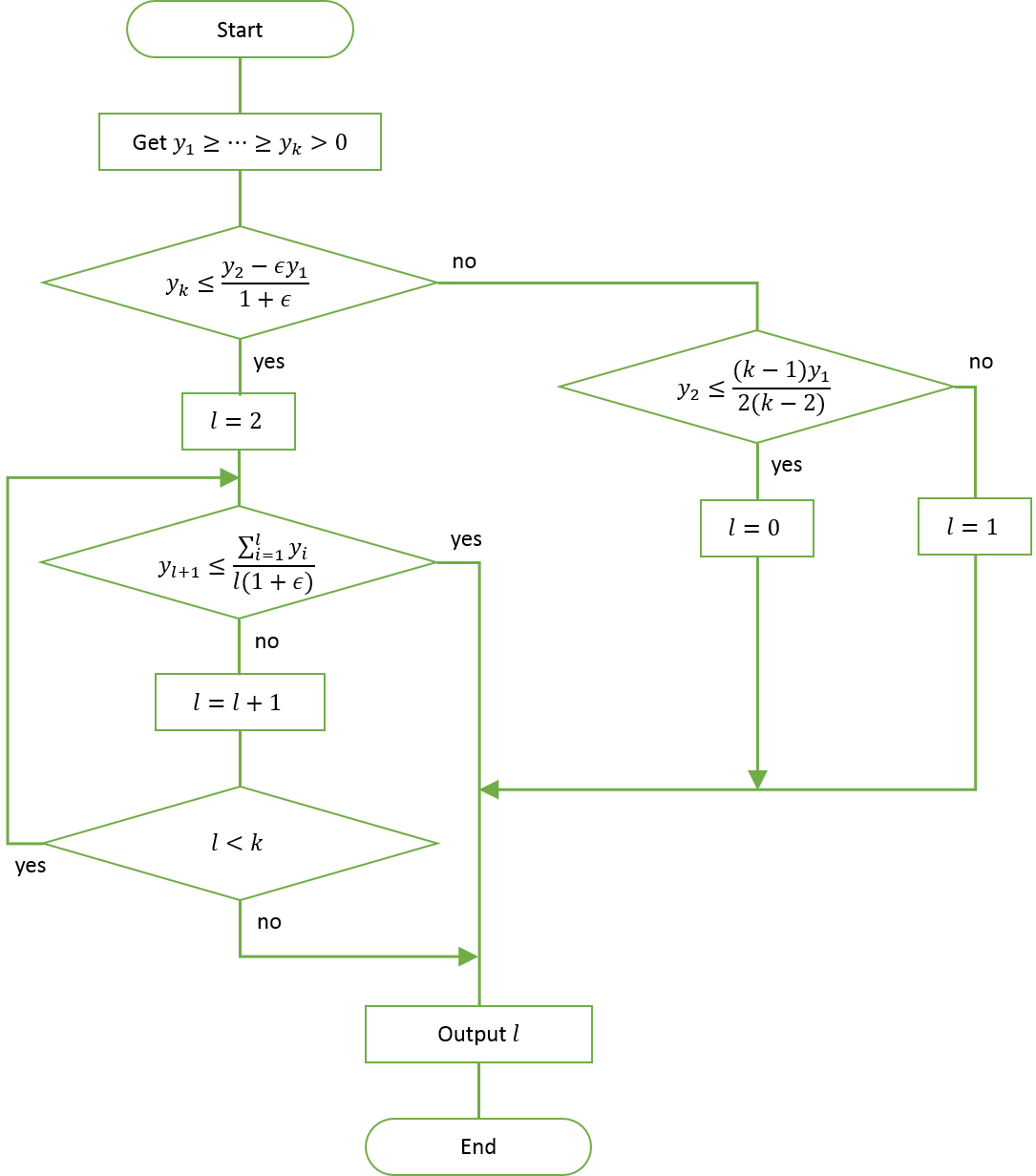
Figure 1: Flowchart to determine $l$.

Because the proof of Lemma 4.3 is long, we postpone proving it until Section 4.3.

4.2 The improved algorithm

Now we show that there exists $\epsilon>0$, which satisfies (24), (25), and (26).

Lemma 4.4.

$\epsilon$, where $0<\epsilon\leq 1/k^{2}$, satisfies (24), (25) and (26).

Proof 4.5.

First, we show the statement for (24). Let $q_{1}(\epsilon)=\frac{\sqrt{2}}{\sqrt{1+\epsilon}}-\frac{\epsilon}{1+\epsilon}-1-\epsilon$. We have $q^{\prime}_{1}(\epsilon)<0$ for $\epsilon>0$. By putting $\epsilon=1/9$, we obtain $q_{1}(1/9)>0$. Hence, from $k\geq 3$, we have $q_{1}(\epsilon)>0$ for $0<\epsilon\leq 1/k^{2}(\leq 1/9)$.

Second, we show the statement for (25). Let $q_{2}(\epsilon)=\frac{1}{k-1}+\frac{1-\epsilon}{1+\epsilon}-1-\epsilon$. We have $q^{\prime}_{2}(\epsilon)<0$ for $\epsilon>0$. By putting $\epsilon=1/3k$, we obtain $q_{2}(1/3k)>0$. Hence, from $k\geq 3$, we have $q_{2}(\epsilon)>0$ for $0<\epsilon\leq 1/k^{2}(\leq 1/3k)$.

Finally, we show the statement for (26). Let $q_{3}(\epsilon)=\frac{1}{k-1}\prod_{j=2}^{k-1}\left(1+\frac{1}{j(1+\epsilon)}\right)-\frac{1+2\epsilon}{2}$. From $\epsilon\geq 0$, we have

$$q_{3}(\epsilon) \geq \frac{1}{k-1}\prod_{j=2}^{k-1}\left\{\frac{1}{1+\epsilon}\left(1+\frac{1}{j}\right)\right\}-\frac{1+2\epsilon}{2}$$

$$= \frac{1}{2}\left\{\frac{k}{k-1}\frac{1}{(1+\epsilon)^{k-2}}-(1+2\epsilon)\right\}$$

$$\geq \frac{k(1+\epsilon)^{2}}{2(k-1)}\left\{\frac{1}{(1+\epsilon)^{k}}-\frac{k-1}{k}\right\}.$$

So $q_{3}(\epsilon)\geq 0$ for $\epsilon\leq\sqrt[k]{\frac{k}{k-1}}-1$. From $\frac{1}{x-1}>\ln(x)-\ln(x-1)>\frac{1}{x}$, we obtain

$$\frac{1}{k}\ln\left(\frac{k}{k-1}\right)>\frac{1}{k^{2}}>\ln\left(\frac{k^{2}+1}{k^{2}}\right).$$

Therefore $1+\frac{1}{k^{2}}<\sqrt[k]{\frac{k}{k-1}}$ holds and we have $q_{3}(\epsilon)\geq 0$ for $\epsilon\leq 1/k^{2}(\leq\sqrt[k]{\frac{k}{k-1}}-1)$.

Now we are ready to show the algorithm.

Algorithm 4 A randomized $k$-submodular function maximization algorithm

1:$\boldsymbol{s}\leftarrow\boldsymbol{0}\ (\boldsymbol{s}\in\{0,1,...,k\}^{V})$.

2:Let $\epsilon$ be the value which satisfies the following equations for $k$:

(24 ) $$\frac{\sqrt{2}}{\sqrt{1+\epsilon}}-\frac{\epsilon}{1+\epsilon}\geq 1+\epsilon,$$

(25) $$\frac{1}{k-1}+\frac{1-\epsilon}{1+\epsilon}\geq 1+\epsilon,$$

(26) $$\frac{1}{k-1}\prod_{j=2}^{k-1}\left(1+\frac{1}{j(1+\epsilon)}\right)\geq\frac{1+2\epsilon}{2}.$$

3:for $t=1,...,n$ do

4:     $y_{i}\leftarrow\Delta_{e,i}f(\boldsymbol{s})\ (i\in[k])$.

5:     Assume $y_{1}\geq y_{2}\geq\cdots\geq y_{k}$.

6:     if $y_{k}<0$ then

7:         $\beta\leftarrow\sum_{i=1}^{k}y_{i}^{k-1}$.

8:          $p_{i}^{(t)}\leftarrow\frac{y_{i}^{k-1}}{\beta}\ (i\leq k-1),\ 0\ (i=k)$.

9:     else

10:         if $y_{k}>\frac{y_{2}-\epsilon y_{1}}{1+\epsilon}$. then

11:              if $y_{2}\leq\frac{k-1}{2(k-2)}y_{1}$ then $l\leftarrow 0$.

12:              else

13:                  $l\leftarrow 1$.

14:              end if

15:         else

16:              $l\leftarrow 2$.

17:              while $l<k\ \text{and}\ y_{l+1}>\frac{\sum_{i=1}^{l}y_{i}}{l(1+\epsilon)}$ do

18:                  $l\leftarrow l+1$.

19:              end while

20:         end if

21:     end if

22:     if $l\geq 2$ then $p_{i}^{(t)}\leftarrow\begin{cases}1/l&(i\leq l)\\ 0&(i>l)\end{cases}$.

23:     else if $l=1$ then $p_{1}^{(t)}\leftarrow 1-\frac{(k-1)y_{2}}{(k-1)y_{1}+y_{2}},p_{i}^{(t)}\leftarrow\frac{y_{2}}{(k-1)y_{1}+y_{2}}\ (i\neq 1)$.

24:     else

25:          $p_{1}^{(t)}\leftarrow 1-\frac{2y_{2}}{y_{1}+2y_{2}},p_{i}^{(t)}\leftarrow\frac{2y_{2}}{(k-1)(y_{1}+2y_{2})}\ (i\neq 1)$.

26:     end if

27:     Let $\boldsymbol{s}(e^{(t)})\in[k]$ be chosen randomly with $\mathrm{Pr}[\boldsymbol{s}(e^{(t)})=i]=p_{i}^{(t)}$.

28:end for

29:return $\boldsymbol{s}$

By Lemma 4.1 and Lemma 4.3, obtain the following theorem.

Theorem 4.6.

For any nonmonotone $k$-submodular function with $k\geq 3$, there is randomized algorithm which satisfies $\frac{k^{2}+1}{2k^{2}+1}$-approximation.

Proof 4.7.

From appropriate permutation $\sigma$, we can set $y_{\sigma(1)}\geq y_{\sigma(2)}\geq\cdots\geq y_{\sigma(k)}$. If $y_{\sigma(k)}>0$, from Theorem 4.3, there are some $\{p_{i}\}$ satisfy $f(\boldsymbol{p})\leq cg(\boldsymbol{p})$ with $c=1-1/k^{2}$. If $y_{\sigma(k)}\leq 0$, from Lemma 4.1, there are some $\{p_{i}\}$ satisfy $f(\boldsymbol{p})\leq cg(\boldsymbol{p})$ with $c=1-\frac{1}{k-1}$. From the definition of $g$, we have $g(\boldsymbol{p})\geq 0$ for any $\boldsymbol{p}$. Therefore, regardless of the sign of $y_{\sigma(k)}$, we can obtain $\{p_{i}\}$ which satisfies $f(\boldsymbol{p})\leq cg(\boldsymbol{p})$ with $c=1-1/k^{2}$.

Then, from Lemma 3.1, we have a randomized $\frac{k^{2}+1}{2k^{2}+1}$-approximation algorithm.

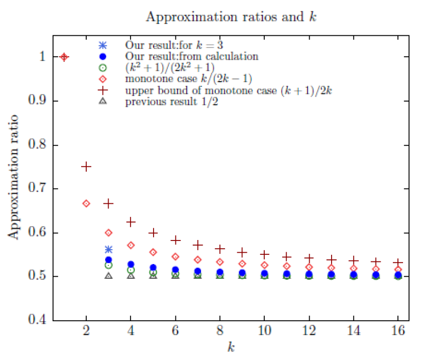
Figure 2: Approximation ratios and $k$

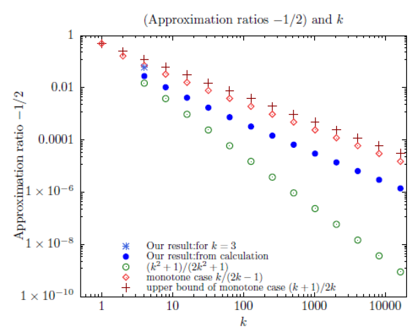
Figure 3: (Approximation ratios - $1/2$) and $k$ in a logarithmic graph

The approximation ratios of our randomized algorithms and previous results are compared in FIG. 2 and FIG. 3. If we use $\epsilon$, which is larger than $1/k^{2}$ and satisfies 24, 25 and 26, we obtain an approximation better than $\frac{k^{2}+1}{2k^{2}+1}$. And $\frac{\sqrt{17}-3}{2}$ is better than the ratio of our algorithm for $k\geq 3$.

4.3 Proof of Lemma 4.3

In this section, we give a proof of Lemma 4.3. From (23), we have $p_{1}\geq\cdots\geq p_{k}\geq 0$. And, from the definition in the statement of Lemma 4.3, we have $y_{i}\geq 0$ for any $i$, and $g(\boldsymbol{p})\geq 0$. Therefore, if $f(\boldsymbol{p})\leq 0$, we have $f(\boldsymbol{p})\leq cg(\boldsymbol{p})$. Hence, from the definition of $f(\boldsymbol{p})$, $f(\boldsymbol{p})\leq cg(\boldsymbol{p})$ holds for the case $a_{i_{-}}<0$ and $i_{-}\neq i^{*}$.

Now suppose $f(\boldsymbol{p})>0$ and $i_{-}\neq i^{*}$ if $a_{i_{-}}<0$. Let

(27) $$\hat{f}(\boldsymbol{p}):=(1-p_{i^{*}})a_{i^{*}}+\max\begin{pmatrix}(1-p_{i^{*}}-2p_{i_{-}})a_{i_{-}},\\ 0\end{pmatrix},$$

We prove

$$\frac{g(\boldsymbol{p})}{f(\boldsymbol{p})}\geq 1+\epsilon.$$

for each $l$. We split the proof according to the value of $l$.

4.3.1 Proof of 4.3 for the case $l=0$

In this section, suppose $l=0$. Let $\alpha=\frac{2\beta}{(k-1)(1+2\beta)}$. Then $\{p_{i}\}$ can be written as

(28) $$p_{1}=1-(k-1)\alpha,\ p_{2}=\cdots=p_{k}=\alpha\ (0\leq\alpha\leq 1/k).$$

Note that $p_{1}\geq p_{2}=\cdots=p_{k}$. It is convenient to have a list of the values of $1-p_{i^{*}}-2p_{i_{-}}$ and $f(\boldsymbol{p})$, for each case of $i^{*}$ and $i_{-}$ on Table 2. For the inequalities in the column of $1-p_{i^{*}}-2p_{i_{-}}$, we used $k\geq 3$ and $p_{1}\geq p_{2}=\cdots=p_{k}$ which follows from the definition. For the inequalities in the column of $f(\boldsymbol{p})$, we used $y_{1}=y_{i^{*}}\geq a_{i^{*}}$ if $i^{*}=1$, $y_{2}\geq y_{i^{*}}\geq a_{i^{*}}$ if $i^{*}\neq 1$ and $|a_{i_{-}}|\leq a_{k}\leq y_{k}$ if $i_{-}\neq k$. These inequalities follow from the definition of $\{p_{i}\}$, (2) and (3). We also have $y_{2}\leq\frac{(k-1)y_{1}}{2(k-2)}$ from the flowchart (FIG 1). Therefore $\alpha=\frac{2\beta}{(k-1)(1+2\beta)}\leq 1/(2k-3)$ holds.

Table 2: $f(\boldsymbol{p})$ in the case $l=0$.

$p_{i^{*}}$	$p_{i_{-}}$	$1-p_{i^{*}}-2p_{i_{-}}$	$f(\boldsymbol{p})$
$1-(k-1)\alpha$	$\alpha$	$(k-3)\alpha\geq 0$	$(k-1)\alpha a_{i^{*}}+(k-3)\alpha a_{i_{-}}$	$\leq$	$(k-1)\alpha y_{1}$
$\alpha$	$1-(k-1)\alpha$	$(2k-3)\alpha-1\leq 0$	$(1-\alpha)a_{i^{*}}+(1-(2k-3)\alpha)|a_{i_{-}}|$
			$\leq(1-\alpha)y_{2}+(1-(2k-3)\alpha)y_{k}$
$\alpha$	$\alpha$	$1-3\alpha>0$	$(1-\alpha)a_{i^{*}}+(1-3\alpha)a_{i_{-}}$	$\leq$	$(1-\alpha)y_{2}$
$1-(k-1)\alpha$	None	None	$(k-1)\alpha a_{i^{*}}$	$\leq$	$(k-1)\alpha y_{1}$
$\alpha$	None	None	$(1-\alpha)a_{i^{*}}$	$\leq$	$(1-\alpha)y_{2}$

By putting $p_{1},...,p_{k}$ in Table 2, we have

$$f(\boldsymbol{p})\leq\begin{cases}(k-1)\alpha y_{1}&(p_{i^{*}}=1-(k-1)\alpha)\\ (1-\alpha)y_{2}+(1-(2k-3)\alpha)y_{k}&(p_{i^{*}}=\alpha)\end{cases}.$$

From $y_{2}\geq y_{k}$,

$$f(\boldsymbol{p})\leq\begin{cases}(k-1)\alpha y_{1}&(p_{i^{*}}=1-(k-1)\alpha)\\ 2(1-(k-1)\alpha)y_{2}&(p_{i^{*}}=\alpha)\end{cases}$$

holds. By putting $\alpha=\frac{2\beta}{(k-1)(1+2\beta)}$, we obtain

$$f(\boldsymbol{p})\leq\frac{2y_{1}\beta}{1+2\beta}.$$

On the other hand, we have

$$g(\boldsymbol{p}) = \left(1-\frac{2\beta}{1+2\beta}\right)y_{1}+\frac{2\beta}{(k-1)(1+2\beta)}(y_{2}+\cdots+y_{k})$$

$$\geq \frac{y_{1}}{1+2\beta}+\frac{2\beta y_{k}}{1+2\beta}$$

$$> \frac{y_{1}}{1+2\beta}+\frac{2\beta}{1+2\beta}\frac{(\beta-\epsilon)y_{1}}{1+\epsilon}$$

by $y_{k}>(y_{2}-\epsilon y_{1})/(1+\epsilon)$, which follows from the flowchart. Therefore,

$$\frac{g(\boldsymbol{p})}{f(\boldsymbol{p})} \geq \frac{1+2\beta(\beta-\epsilon)/(1+\epsilon)}{2\beta}$$

$$= \frac{1}{2\beta}+\frac{\beta}{1+\epsilon}-\frac{\epsilon}{1+\epsilon}$$

holds.

Let $h_{0}(\beta)=\frac{1}{2\beta}+\frac{\beta}{1+\epsilon}-\frac{\epsilon}{1+\epsilon}$. From the definition, $\beta=\frac{y_{2}}{y_{1}}\geq 0$ and $h_{0}$ is minimized when $\beta^{2}=(1+\epsilon)/2$ for $\beta\geq 0$. Then we have

$$\min h_{0}(\beta)=\frac{\sqrt{2}}{\sqrt{1+\epsilon}}-\frac{\epsilon}{1+\epsilon}.$$

From (24), the definition of $\epsilon$, we have $\frac{g(\boldsymbol{p})}{f(\boldsymbol{p})}\geq 1+\epsilon$.

4.3.2 Proof of 4.3 for the case $l=0$

In this section, suppose $l=1$. Let $\alpha=\frac{\beta}{(k-1)+\beta}$. Then $\{p_{i}\}$ can be written as

(28) $$p_{1}=1-(k-1)\alpha,\ p_{2}=\cdots=p_{k}=\alpha\ (0\leq\alpha\leq 1/k).$$

Note that $p_{1}\geq p_{2}=\cdots=p_{k}$. It is convenient to have a list of the values of $1-p_{i^{*}}-2p_{i_{-}}$ and $f(\boldsymbol{p})$, for each case of $i^{*}$ and $i_{-}$ on Table 3. For the inequalities in the column of $1-p_{i^{*}}-2p_{i_{-}}$, we used $k\geq 3$ and $p_{1}\geq p_{2}=\cdots=p_{k}$ which follows from the definition. For the inequalities in the column of $f(\boldsymbol{p})$, we used $y_{1}=y_{i^{*}}\geq a_{i^{*}}$ if $i^{*}=1$ and $y_{2}\geq y_{i^{*}}\geq a_{i^{*}}$ if $i^{*}\neq 1$. These inequalities follow from the definition of $\{p_{i}\}$ and (2). We also have $y_{2}>\frac{(k-1)y_{1}}{2(k-2)}$ from the flowchart (FIG 1). Therefore $\alpha=\frac{\beta}{(k-1)+\beta}>1/(2k-3)$ holds.

Table 3: $f(\boldsymbol{p})$ in the case $l=1$.

$p_{i^{*}}$	$p_{i_{-}}$	$1-p_{i^{*}}-2p_{i_{-}}$	$f(\boldsymbol{p})$
$1-(k-1)\alpha$	$\alpha$	$(k-3)\alpha\geq 0$	$(k-1)\alpha a_{i^{*}}+(k-3)\alpha a_{i_{-}}$	$\leq$	$(k-1)\alpha y_{1}$
$\alpha$	$1-(k-1)\alpha$	$(2k-3)\alpha-1>0$	$(1-\alpha)a_{i^{*}}+\{(2k-3)\alpha-1\}a_{i_{-}}$	$\leq$	$(1-\alpha)y_{2}$
$\alpha$	$\alpha$	$1-3\alpha>0$	$(1-\alpha)a_{i^{*}}+(1-3\alpha)a_{i_{-}}$	$\leq$	$(1-\alpha)y_{2}$
$1-(k-1)\alpha$	None	None	$(k-1)\alpha a_{i^{*}}$	$\leq$	$(k-1)\alpha y_{1}$
$\alpha$	None	None	$(1-\alpha)a_{i^{*}}$	$\leq$	$(1-\alpha)y_{2}$

In Table 3, we have

$$f(\boldsymbol{p})\leq\begin{cases}(k-1)\alpha y_{1}&(p_{i^{*}}=1-(k-1)\alpha)\\ (1-\alpha)y_{2}&(p_{i^{*}}=\alpha)\end{cases}.$$

By putting $\alpha=\frac{\beta}{(k-1)+\beta}$,

$$f(\boldsymbol{p})\leq\frac{(k-1)\beta y_{1}}{(k-1)+\beta}.$$

We also have

$$g(\boldsymbol{p}) = \left(1-\frac{(k-1)\beta}{(k-1)+\beta}\right)y_{1}+\frac{\beta}{(k-1)+\beta}(y_{2}+\cdots+y_{k})$$

$$\geq \frac{\{(k-1)-(k-2)\beta\}y_{1}}{(k-1)+\beta}+\frac{(k-1)\beta y_{k}}{(k-1)+\beta}$$

$$> \frac{\{(k-1)-(k-2)\beta\}y_{1}}{(k-1)+\beta}+\frac{(k-1)\beta}{(k-1)+\beta}\frac{(\beta-\epsilon)y_{1}}{1+\epsilon}$$

by $y_{k}>(y_{2}-\epsilon y_{1})/(1+\epsilon)$ which follows from the flowchart. Hence

$$\frac{g(\boldsymbol{p})}{f(\boldsymbol{p})} \geq \frac{(k-1)-(k-2)\beta+(k-1)\beta(\beta-\epsilon)/(1+\epsilon)}{(k-1)\beta}$$

$$= \frac{1}{\beta}-\frac{k-2}{k-1}+\frac{\beta}{1+\epsilon}-\frac{\epsilon}{1+\epsilon}$$

holds.

Let $h_{1}(\beta)=\frac{1}{\beta}-\frac{k-2}{k-1}+\frac{\beta}{1+\epsilon}-\frac{\epsilon}{1+\epsilon}$. From $\epsilon>0$ and $\beta\leq 1$, which follows from the definitions, $h_{1}(\beta)$ is minimized when $\beta=1$. Then we have

$$\min h_{1}(\beta)=\frac{1}{k-1}+\frac{1-\epsilon}{1+\epsilon}.$$

From (24), the definition of $\epsilon$, we have $\frac{g(\boldsymbol{p})}{f(\boldsymbol{p})}\geq 1+\epsilon$.

4.3.3 Proof of 4.3 for the case $l=2$

In this section, suppose $l=2$. We have $p_{1}=p_{2}=1/2,p_{3}=\cdots=p_{k}=0$ from (23). It is convenient to have a list of the values of $1-p_{i^{*}}-2p_{i_{-}}$ and $f(\boldsymbol{p})$, for each case of $i^{*}$ and $i_{-}$ on Table 4. For the inequalities in the column of $f(\boldsymbol{p})$, we used $y_{i}\geq a_{i}(i\in[k])$ and $a_{i}+a_{j}\geq 0$, which follows from the definition (2) and (3).

Table 4: $f(\boldsymbol{p})$ in the case $l=2$

$p_{i^{*}}$	$p_{i_{-}}$	$1-p_{i^{*}}-2p_{i_{-}}$	$f(\boldsymbol{p})$
$1/2$	$1/2$	$-1/2<0$	$(a_{i^{*}}-a_{i_{-}})/2$	$\leq$	$(y_{1}+y_{k})/2$
$1/2$	$0$	$1/2>0$	$(a_{i^{*}}+a_{i_{-}})/2$	$\leq$	$y_{1}/2$
$0$	$1/2$	$0$	$a_{i^{*}}$	$\leq$	$y_{3}$
$0$	$0$	$1>0$	$a_{i^{*}}+a_{i_{-}}$	$\leq$	$y_{3}$
$1/2$	None	None	$a_{i^{*}}/2$	$\leq$	$y_{1}/2$
$0$	None	None	$a_{i^{*}}$	$\leq$	$y_{3}$

In Table 4, from $y_{k}>0$, we obtain

$$f(\boldsymbol{p})\leq\begin{cases}(y_{1}+y_{k})/2&(p_{i^{*}}=1/2)\\ y_{3}&(p_{i^{*}}=0)\end{cases}.$$

We also have $g(\boldsymbol{p})=(y_{1}+y_{2})/2$, and then

(29) $$\frac{g(\boldsymbol{p})}{f(\boldsymbol{p})}\geq\min\left\{\frac{y_{1}+y_{2}}{y_{1}+y_{k}},\frac{y_{1}+y_{2}}{2y_{3}}\right\}$$

holds. From the flowchart, we obtain $y_{k}\leq\frac{y_{2}-\epsilon y_{1}}{1+\epsilon}$, $y_{1}+y_{k}\leq\frac{y_{1}+y_{2}}{1+\epsilon}$ and $y_{3}\leq\frac{y_{1}+y_{2}}{2(1+\epsilon)}$. By these inequalities and (29), we get $g(\boldsymbol{p})/f(\boldsymbol{p})\geq 1+\epsilon$．

4.3.4 Proof of 4.3 for the case $3\leq l\leq k-1$

Now suppose $3\leq l\leq k-1$. We have $p_{1}=\cdots=p_{l}=1/l,\ p_{l+1}=\cdots=p_{k}=0$ from (23). From $l\geq 3$, we obtain $1-p_{i^{*}}-2p_{i_{-}}\geq 0$. Therefore, $(1-p_{i^{*}}-2p_{i_{-}})a_{i_{-}}\leq 0$ holds and we obtain $f(\boldsymbol{p})\leq(1-p_{i^{*}})a_{i^{*}}$. It is convenient to have a list of the values of $f(\boldsymbol{p})$, for each case of $i^{*}$ and $i_{-}$ on Table 5. For the inequalities in the column of $f(\boldsymbol{p})$, we used $y_{i}\geq a_{i}(i\in[k])$, which follows from the definition (2).

Table 5: $f(\boldsymbol{p})$ in the case $3\leq l\leq k-1$

$p_{i^{*}}$	$f(\boldsymbol{p})$
$1/l$	$f(\boldsymbol{p})$	$\leq(1-1/l)a_{i^{*}}$	$\leq(1-1/l)y_{1}$
$0$	$f(\boldsymbol{p})$	$\leq a_{i^{*}}$	$\leq y_{l+1}$

In table 5, we have $f(\boldsymbol{p})\leq\max\{(1-1/l)y_{1},y_{l+1}\}$ and $g(\boldsymbol{p})=(\sum_{i=1}^{l}y_{i})/l$. Hence

$$\frac{g(\boldsymbol{p})}{f(\boldsymbol{p})}\geq\min\left\{\frac{\sum_{i=1}^{l}y_{i}}{(l-1)y_{1}},\frac{\sum_{i=1}^{l}y_{i}}{l\cdot y_{l+1}}\right\}$$

holds.

From the flowchart, we have $y_{l+1}\leq\frac{\sum_{i=1}^{l}y_{i}}{l(1+\epsilon)}$. Otherwise, we obtain $l+1$ as the output of the flowchart. So we have

$$\frac{\sum_{i=1}^{l}y_{i}}{l\cdot y_{l+1}}\geq 1+\epsilon.$$

Now we need to show

$$\frac{\sum_{i=1}^{l}y_{i}}{(l-1)y_{1}}\geq 1+\epsilon.$$

From the flowchart, we also have $y_{l^{\prime}+1}>\frac{\sum_{i=1}^{l^{\prime}}y_{i}}{l^{\prime}(1+\epsilon)}$ for any $l^{\prime}$ which satisfies $2\leq l^{\prime}<l$. Otherwise, we obtain $l^{\prime}<l$ as the output of the flowchart. Hence we have

$$\sum_{i=1}^{l}y_{i} = \sum_{i=1}^{l-1}y_{i}+y_{l}$$

$$> \sum_{i=1}^{l-1}y_{i}+\frac{\sum_{i=1}^{l-1}y_{i}}{(l-1)(1+\epsilon)}=\left(1+\frac{1}{(l-1)(1+\epsilon)}\right)\sum_{i=1}^{l-1}y_{i}$$

$$> \cdots>\left[\prod_{j=2}^{l-1}\left(1+\frac{1}{j(1+\epsilon)}\right)\right](y_{1}+y_{2}).$$

By $y_{2}\geq y_{3}>\frac{y_{1}+y_{2}}{2(1+\epsilon)}$, we also have $y_{2}>y_{1}/(1+2\epsilon)$. From these inequalities, we obtain

$$\sum_{i=1}^{l}y_{i}>\left[\prod_{j=2}^{l-1}\left(1+\frac{1}{j(1+\epsilon)}\right)\right]\cdot\frac{2(1+\epsilon)}{1+2\epsilon}y_{1}.$$

Hence

$$\frac{\sum_{i=1}^{l}y_{i}}{(l-1)y_{1}}>\frac{1}{l-1}\left[\prod_{j=2}^{l-1}\left(1+\frac{1}{j(1+\epsilon)}\right)\right]\frac{2(1+\epsilon)}{1+2\epsilon}$$

holds.

Let $f(l)=\frac{1}{l-1}\prod_{j=2}^{l-1}\left(1+\frac{1}{j(1+\epsilon)}\right)$. Then we have

$$f(l)=\frac{l-2}{l-1}\left(1+\frac{1}{(l-1)(1+\epsilon)}\right)f(l-1)=\left\{1-\frac{1+(l-1)\epsilon}{(l-1)^{2}(1+\epsilon)}\right\}f(l-1).$$

From $\epsilon>0$, we have $f(l)<f(l-1)$ and $f(k)<f(l)$ for $3\leq l\leq k$. Hence we have $\frac{\sum_{i=1}^{l}y_{i}}{(l-1)y_{1}}\geq 1+\epsilon$ for $3\leq l\leq k$ from the definition of $\epsilon$ (26).

4.3.5 Proof of 4.3 for the case $l=k$

In this section, suppose $l=k$. We have $p_{1}=\cdots=p_{k}=1/k$ from (23). From $l=k\geq 3$, we obtain $1-p_{i^{*}}-2p_{i_{-}}\geq 0$. Therefore, $(1-p_{i^{*}}-2p_{i_{-}})a_{i_{-}}\leq 0$ holds and we obtain $f(\boldsymbol{p})\leq(1-p_{i^{*}})a_{i^{*}}$. By putting $p_{i}=1/k$ and $y_{1}\geq y_{i}\geq a_{i}$ for $i\in[k]$, which follows from the definition (2), we have $f(\boldsymbol{p})\leq\frac{k-1}{k}y_{1}$. We also have $g(\boldsymbol{p})=(\sum_{i=1}^{k}y_{i})/k$. Hence we obtain

$$\frac{g(\boldsymbol{p})}{f(\boldsymbol{p})}\geq\frac{\sum_{i=1}^{k}y_{i}}{(k-1)y_{1}}.$$

From the flowchart, we have $y_{l^{\prime}+1}>\frac{\sum_{i=1}^{l^{\prime}}y_{i}}{l^{\prime}(1+\epsilon)}$ for any $2\leq l^{\prime}<k$. Otherwise, we obtain $l^{\prime}<k$ as the output of the flowchart. In the same way as the discussion in the previous section, we have

$$\frac{\sum_{i=1}^{k}y_{i}}{(k-1)y_{1}}>\frac{1}{k-1}\left[\prod_{j=2}^{k-1}\left(1+\frac{1}{j(1+\epsilon)}\right)\right]\frac{2(1+\epsilon)}{1+2\epsilon}.$$

From (26), the definition of $\epsilon$, we have $\frac{\sum_{i=1}^{k}y_{i}}{(k-1)y_{1}}\geq 1+\epsilon$.

5 Conclusion

We proposed two randomized algorithms for nonmonotone $k$-submodular maximization with $k\geq 3$. Our general algorithm achieves a better approximation ratio, $\frac{k^{2}+1}{2k^{2}+1}$, for $k\geq 3$ we can even get a better algorithm.

It might be possible to analyze the case $k\geq 4$ similarly to the case $k=3$. However generalization is difficult. It is interesting that there is a systematic way to improve an approximation ratio for $k\geq 4$ or not.

References

- [1] N. Buchbinder and M. Feldman, Deterministic algorithms for submodular maximization problems, in Proceedings of the Twenty-Seventh Annual ACM-SIAM Symposium on Discrete Algorithms, SIAM, 2016, pp. 392–403.
- [2] N. Buchbinder, M. Feldman, J. Naor, and R. Schwartz, A tight linear time (1/2)-approximation for unconstrained submodular maximization, SIAM Journal on Computing, 44 (2015), pp. 1384–1402.
- [3] U. Feige, V. S. Mirrokni, and J. Vondrák, Maximizing non-monotone submodular functions, SIAM Journal on Computing, 40 (2011), pp. 1133–1153.
- [4] A. Frank, An algorithm for submodular functions on graphs, Annals of Discrete Mathematics, 16 (1982), pp. 97–120.
- [5] S. Fujishige, Theory of submodular programs: A fenchel-type min-max theorem and subgradients of submodular functions, Mathematical programming, 29 (1984), pp. 142–155.
- [6] I. Gridchyn and V. Kolmogorov, Potts model, parametric maxflow and k-submodular functions, in Proceedings of the IEEE International Conference on Computer Vision, 2013, pp. 2320–2327.
- [7] M. Grötschel, L. Lovász, and A. Schrijver, The ellipsoid method and its consequences in combinatorial optimization, Combinatorica, 1 (1981), pp. 169–197.
- [8] A. Huber and V. Kolmogorov, Towards minimizing k-submodular functions, in International Symposium on Combinatorial Optimization, Springer, 2012, pp. 451–462.
- [9] S. Iwata, L. Fleischer, and S. Fujishige, A combinatorial strongly polynomial algorithm for minimizing submodular functions, Journal of the ACM, 48 (2001), pp. 761–777.
- [10] S. Iwata, S. Tanigawa, and Y. Yoshida, Bisubmodular function maximization and extensions, tech. report, METR 2013-16, The University of Tokyo, 2013.
- [11] S. Iwata, S. Tanigawa, and Y. Yoshida, Improved approximation algorithms for k-submodular function maximization, in Proceedings of the Twenty-Seventh Annual ACM-SIAM Symposium on Discrete Algorithms, SIAM, 2016, pp. 404–413.
- [12] L. Lovász, Submodular functions and convexity, in Mathematical Programming The State of the Art, A. Bachem, M. Grötschel, and B. Korte, eds., Springer, Heidelberg, 1983, pp. 235–257.
- [13] N. Ohsaka and Y. Yoshida, Monotone k-submodular function maximization with size constraints, in Advances in Neural Information Processing Systems, 2015, pp. 694–702.
- [14] A. Schrijver, A combinatorial algorithm minimizing submodular functions in strongly polynomial time, Journal of Combinatorial Theory, Series B, 80 (2000), pp. 346–355.
- [15] J. Ward and S. Živný, Maximizing k-submodular functions and beyond, ACM Transactions on Algorithms, 12 (2016), pp. 47:1–47:26.