Non-Markovian barrier crossing with two-time-scale memory is dominated by the faster memory component

Abstract

We investigate non-Markovian barrier-crossing kinetics of a massive particle in one dimension in the presence of a memory function that is the sum of two exponentials with different memory times $\tau_{1}$ and $\tau_{2}$. Our Langevin simulations for the special case where both exponentials contribute equally to the total friction show that the barrier crossing time becomes independent of the longer memory time if at least one of the two memory times is larger than the intrinsic diffusion time. When we associate memory effects with coupled degrees of freedom that are orthogonal to a one-dimensional reaction coordinate, this counterintuitive result shows that the faster orthogonal degrees of freedom dominate barrier-crossing kinetics in the non-Markovian limit and that the slower orthogonal degrees become negligible, quite contrary to the standard time-scale separation assumption and with important consequences for the proper setup of coarse-graining procedures in the non-Markovian case. By asymptotic matching and symmetry arguments, we construct a crossover formula for the barrier crossing time that is valid for general multi-exponential memory kernels. This formula can be used to estimate barrier-crossing times for general memory functions for high friction, i.e. in the overdamped regime, as well as for low friction, i.e. in the inertial regime. Typical examples where our results are important include protein folding in the high-friction limit and chemical reactions such as proton-transfer reactions in the low-friction limit.

I Introduction

Rare events, such as chemical reactions, macromolecular conformational transitions, or nucleation events, can be modeled as barrier crossing in an effective one-dimensional energy landscape Kramers (1940); Chandler (1986); Berne et al. (1988); Hänggi et al. (1990); Best and Hummer (2006). Due to the coupling to intra- and intermolecular orthogonal degrees of freedom, the dynamics of the reaction coordinate becomes non-Markovian and can be characterized by a memory function that describes for how long a system remembers its past state Zwanzig (1961); Mori (1965); Jung et al. (2017, 2018); Meyer et al. (2017, 2019). Memory effects have been studied in the context of ion-pair kinetics Rey and Guardia (1992); Mullen et al. (2014), conformational transitions in small molecules Rosenberg et al. (1980); de Sancho et al. (2014); Daldrop et al. (2018a), diffusive motion of particles and molecules in liquids Mason and Weitz (1995); Lesnicki et al. (2016); Daldrop et al. (2017); Berner et al. (2018), cell locomotion Selmeczi et al. (2005), polymer looping kinetics Wilemski and Fixman (1974); Szabo et al. (1980); Dua and Adhikari (2011); Gowdy et al. (2017); Guérin et al. (2012) and protein folding Plotkin and Wolynes (1998); Das and Makarov (2018), and have been demonstrated to substantially influence barrier-crossing times for slowly decaying memory functions Grote and Hynes (1980); Carmeli and Nitzan (1982); Straub et al. (1986); Talkner and Braun (1988); Pollak et al. (1989); Ianconescu and Pollak (2015).

In previous numerical studies concerned with position-independent memory effects on the barrier-crossing kinetics, the memory function has been assumed to be single exponential or single Gaussian and is thus chraracterized by a single time scale, the memory time $\tau_{\Gamma}$ Straub et al. (1986); Pollak et al. (1989); Tucker et al. (1991); Ianconescu and Pollak (2015); Kappler et al. (2018). Even in this simple scenario the effect memory has on the time needed to cross the barrier, the mean-first passage time $\tau_{\mathrm{MFP}}$, is subtle: for a memory time $\tau_{\Gamma}$ that is longer than the intrinsic diffusion time scale and for fixed friction coefficient $\gamma$ (defined by the integral over the memory function), $\tau_{\mathrm{MFP}}$ scales as $\tau_{\mathrm{MFP}}\sim\tau_{\Gamma}^{2}{\rm e}^{\beta U_{0}}$, where $U_{0}$ denotes the barrier height and $\beta=1/(k_{\mathrm{B}}T)$ the inverse thermal energy Straub et al. (1986); Kappler et al. (2018). The exponential term corresponds to the Arrhenius law and is for many applications the dominant factor. In the present context we are mostly interested in the pre-exponential factor, which signals that the presence of memory modifies the barrier-crossing kinetics even when the barrier-crossing time $\tau_{\mathrm{MFP}}$ is much longer than the memory time $\tau_{\Gamma}$; thus, a naive time-scale separation argument, according to which memory would only influence reaction kinetics up to times scales of the memory time itself, is not valid. For intermediate values of $\tau_{\Gamma}$ a distinct scaling regime exists, where memory in fact speeds up barrier-crossing kinetics, meaning that $\tau_{\mathrm{MFP}}$ is significantly shorter than in the Markovian limit when $\tau_{\Gamma}$ tends to zero at fixed $\gamma$ Kappler et al. (2018). Thus, i) whether memory speeds up or slows down reaction kinetics depends on the precise value of the memory time, and ii) for long memory time $\tau_{\Gamma}$ the barrier-crossing time $\tau_{\mathrm{MFP}}$ is influenced by memory effects even when $\tau_{\mathrm{MFP}}\gg\tau_{\Gamma}$.

While these results vividly demonstrate the complex influence of memory on reaction kinetics, they are of only limited practical use, since memory effects are typically caused by the reaction coordinate coupling to several orthogonal degrees of freedom and as a consequence memory functions are characterized by more than one time scale Rey and Guardia (1992); Tolokh et al. (2002); de Sancho et al. (2014); Lesnicki et al. (2016); Gottwald et al. (2015); Daldrop et al. (2017). Systematic numerical results on the effect of memory functions with more than one time scale on reaction kinetics have not been presented in literature.

In this work, we study the barrier-crossing dynamics of a massive particle in a one-dimensional double-well potential in the presence of a memory function that consists of the sum of two exponentials with different decay times $\tau_{1}$ and $\tau_{2}$. To limit the number of parameters in our simulations of the generalized Langevin equation (GLE), we consider the case where the two exponentials each contribute equally to the friction coefficient, i.e. when the integrals over each memory component are equal. Contrary to what one might intuitively expect, we find that in the asymmetric case $\tau_{1}\ll\tau_{2}$, the barrier-crossing time is solely determined by the memory contribution with the shorter memory time $\tau_{1}$ if $\tau_{2}$ exceeds the intrinsic diffusion time scale; this result is also predicted analytically by a pole analysis of the linearized Langevin equation. Our finding is at odds with standard time scale separation arguments and coarse graining procedures that are normally designed to project onto the slowest degrees of freedom Northrup and Hynes (1980); Zwanzig (1973); Baron et al. (2007); Potoyan et al. (2013). We conclude that for non-Markovian barrier-crossing phenomena, in particular the coupling to the fast – not the slow – orthogonal degrees of freedom needs to be preserved in order to obtain an accurate description of the reaction kinetics.

Based on symmetry arguments and asymptotically valid rate expressions, we construct a heuristic crossover formula for the barrier-crossing time in a double well potential in the presence of a general multi-exponential memory kernel. This crossover formula not only accurately describes our numerical results for bi-exponential memory functions, it can also be used to estimate the effects general memory functions have on the reaction kinetics of experimental and simulation systems.

Our results are relevant for the description of the reaction kinetics of general non-Markovian systems. For example, pronounced memory effects are expected when the folding of a protein is described in terms of a reaction coordinate that does not properly describe all barriers relevant for the folding process Plotkin and Wolynes (1998). The traditional approach would be to construct an improved reaction coordinate that shows minimal memory effects. We here consider an alternative modeling approach that includes non-Markovian effects, and in particular the fast-decaying memory contributions in order to correctly describe the reaction kinetics. One other example where strong memory effects are expected are fast chemical reactions in a solvent, for example proton-transfer reactions in water, where the motion along the reaction coordinate and solvent motion occur on the same time scale Marx et al. (1999); Daldrop et al. (2018b). Also here, a reduced description in terms of a low-dimensional reaction coordinate becomes valid if memory effects are properly included. Again, the quickly decaying memory contributions will be particularly important. Our paper is a first step towards the systematic usage of multi-scale memory functions for non-Markovian kinetic modeling.

II Model for barrier crossing with two-time-scale memory

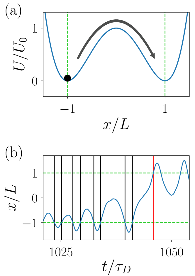
Figure 1: (a) Illustration of the barrier crossing of a massive particle in the double-well potential $U(x)$ given by Eq. (2). The mean first-passage time $\tau_{\mathrm{MFP}}$ is defined as the mean time difference between crossing the minimum at $x=-L$ (left dashed line) and crossing the other minimum at $x=L$ (right dashed line) for the first time. (b) Illustration of how first-passage times (FPTs) are obtained from Langevin simulations. Vertical black lines mark crossings of the trajectory with the potential minimum $x=-L$ (lower dashed horizontal line), the vertical red line marks the first crossing of the trajectory with the potential minimum $x=L$ (upper dashed horizontal line). Each vertical black line contributes to the ensemble of first-passage events and the corresponding FPT is obtained by calculating the time difference between the black and the red lines. The MFPT $\tau_{\mathrm{MFP}}$ is obtained by averaging over all FPTs. For the simulation trajectory shown, the parameters $\tau_{m}/\tau_{D}=10$, $\tau_{1}/\tau_{D}=\tau_{2}/\tau_{D}=0.001$ and barrier height $\beta U_{0}=3$ are used.

We consider the one-dimensional generalized Langevin equation (GLE) Zwanzig (1961); Mori (1965); Grote and Hynes (1980); Pollak et al. (1989)

$$m\,\ddot{x}(t)=-\int_{0}^{t}\Gamma(t-t^{\prime})\dot{x}(t^{\prime})\,\mathrm{d}t^{\prime}-U^{\prime}(x(t))+\eta(t),$$ (1)

where $m$ is the effective mass of the reaction coordinate $x$, $\Gamma(t)$ is the memory function, $U^{\prime}(x)$ denotes the derivative of the potential $U(x)$, and $\eta(t)$ is a time-dependent random force. The random force is Gaussian with zero mean, $\langle\eta(t)\rangle=0$, and obeys the generalized fluctuation-dissipation theorem (FDT) $\beta\left\langle\eta(t)\eta(t^{\prime})\right\rangle=\Gamma(|t-t^{\prime}|)$. We consider a symmetric double-well potential

$$U(x)=U_{0}\left[\left(\frac{x}{L}\right)^{2}-1\right]^{2},$$ (2)

illustrated in Fig. 1 (a), which is characterized by the barrier height $U_{0}$ and by the spatial separation $2L$ between the two potential wells. In our simulations we assume a bi-exponential memory function

$$\Gamma(t) =\sum_{i=1}^{2}\frac{\gamma_{i}}{\tau_{i}}\exp\left(-{|t|}/{\tau_{i}}\right)$$ (3)

where $\tau_{1}$, $\tau_{2}$ are two memory time scales and the corresponding friction coefficients are $\gamma_{1}$, $\gamma_{2}$. We call $\gamma=\int_{0}^{\infty}\mathrm{d}t\,\Gamma(t)=\gamma_{1}+\gamma_{2}$ the total friction coefficient. In our simulations we consider the special case where each of the two exponentials contributes equally to the total friction coefficient, i.e. $\gamma_{1}=\gamma_{2}=\gamma/2$. To reduce the number of parameters, we introduce the time scales

$$\tau_{m}=\frac{m}{\gamma},\qquad\qquad\tau_{D}=\beta L^{2}\gamma,$$ (4)

where the inertial time $\tau_{m}$ characterizes viscous dissipation of particle momentum, and $\tau_{D}$ is the intrinsic diffusion time which depends on the barrier separation $L$ and the total friction coefficient $\gamma$. Memory effects are important if the memory time exceeds $\tau_{D}$. With these definitions, the bi-exponential system with $\gamma_{1}=\gamma_{2}=\gamma/2$ is determined by the three dimensionless time scale ratios $\tau_{m}/\tau_{D}$, $\tau_{1}/\tau_{D}$, $\tau_{2}/\tau_{D}$ and the dimensionless barrier height $\beta U_{0}$, see Appendix A for details. In our simulations we use a fixed barrier height of $\beta U_{0}=3$, except in Appendix G where we also present results for higher values of $\beta U_{0}$.

To simulate the GLE numerically, we explicitly couple the particle coordinate $x$ to two auxiliary degrees of freedom with relaxation times $\tau_{1}$ and $\tau_{2}$, see Appendix B for details. Using a fourth-order Runge-Kutta integration scheme, we then simulate the composite system in the parameter range $\tau_{m}/\tau_{D}\in[10^{-3},10^{3}]$, $\tau_{1}/\tau_{D},\tau_{2}/\tau_{D}\in[10^{-3},10^{2}]$. Initial particle positions are sampled from a Gaussian approximation of the probability distribution in the left well around $x=-L$, i.e., $\langle x(0)\rangle=-L$, $\beta\langle(x(0)+L)^{2}\rangle=1/U^{\prime\prime}(-L)=L^{2}/(8U_{0})$. Initial velocities are sampled from a Gaussian distribution with zero mean and variance $\beta\langle\dot{x}^{2}(0)\rangle=1/m$, in accordance with the equipartition theorem. The initial values for the auxiliary degrees of freedom are sampled from their corresponding equilibrium distributions, see Appendix B for details.

From our simulations we obtain distributions for the first-passage time (FPT) $\tau_{\mathrm{FP}}$ defined by the time difference between crossing the potential minimum at $x=-L$ and reaching the potential minimum at $x=L$ for the first time, see Fig. 1 (b) for an illustration. Since the potential is symmetric, we also collect first-passage events from crossing $x=L$ and reaching $x=-L$ for the first time. The mean first-passage time (MFPT) $\tau_{\mathrm{MFP}}$ is subsequently calculated by averaging over all individual first-passage events.

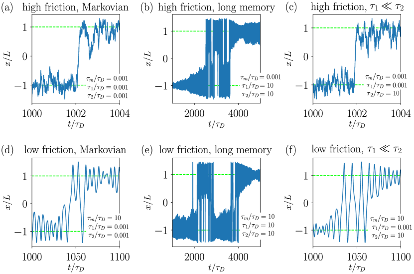
Figure 2: Typical simulation trajectories that display barrier-crossing events for fixed barrier height $\beta U_{0}=3$. Simulation parameters used are given in the legends. The horizontal dashed lines indicate the minima of the quartic potential Eq. (2), which is shown in Fig. 1 (a).

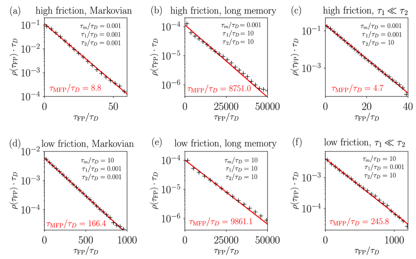
Figure 3: First-passage time (FPT) distributions $\rho(\tau_{\mathrm{FP}})$ for barrier crossing from one potential well to the other. Simulation parameters are given in the legends. For each subplot, first-passage events are obtained from the numerical simulations as illustrated in Fig. 1 (b). The resulting normalized probability distribution $\rho(\tau_{\mathrm{FP}})$ is shown as black crosses. The MFPT value $\tau_{\mathrm{MFP}}$ given in the plots is obtained by averaging over all first-passage events, and used to plot an exponential distribution as defined in Eq. (5), shown as a solid line.

III Trajectories and first-passage distributions

In Fig. 2 we show typical simulation trajectories that illustrate how the character of barrier-crossing events changes with varying mass, friction, and memory time parameters. In Fig. 2 (a), (b), (d), (e) the two memory times are equal, $\tau_{\Gamma}\equiv\tau_{1}=\tau_{2}$, so that the memory function is in fact single-exponential. For high friction and short memory in Fig. 2 (a), i.e. for $\tau_{m}/\tau_{D}\ll 1$ and $\tau_{\Gamma}/\tau_{D}\ll 1$, the barrier crossing is diffusive, meaning that the particle fluctuates in a potential well for a long time until a single barrier-crossing event occurs with a transition path time that is much shorter than the mean first-passage time Chung and Eaton (2013); Laleman et al. (2017). In contrast, if the friction is low or if the memory time is long, i.e. for $\tau_{m}/\tau_{D}\gg 1$ or $\tau_{\Gamma}/\tau_{D}\gg 1$, the trajectories in Fig. 2 (b), (d), (e) are characterized by bursts of multiple barrier recrossings. In these cases the barrier-crossing dynamics is dominated by the diffusive exchange of energy between the particle and the thermal bath; once the particle has acquired enough energy to cross the barrier, it oscillates back and forth between the two wells until its energy falls below the barrier energy again Mel’nikov and Meshkov (1986); Kappler et al. (2018). Figure 2 (c) shows a trajectory for high friction $\tau_{m}/\tau_{D}=0.001\ll 1$ and different memory times $\tau_{1}/\tau_{D}=0.001\ll\tau_{2}/\tau_{D}=10$. The trajectory looks similar to the high-friction short-memory trajectory for $\tau_{m}/\tau_{D}=0.001$ and $\tau_{1}/\tau_{D}=\tau_{2}/\tau_{D}=0.001$ shown in Fig. 2 (a), and is markedly different from the trajectory for $\tau_{m}/\tau_{D}=0.001$ and $\tau_{1}/\tau_{D}=\tau_{2}/\tau_{D}=10$ displayed in Fig. 2 (b), which is characterized by extended periods of multiple recrossings. We conclude that a high-friction trajectory that is governed by the sum of a slowly decaying memory contribution with $\tau_{2}/\tau_{D}=10$ and a quickly decaying memory contribution with $\tau_{1}/\tau_{D}=0.001$ looks like a trajectory with only short-time memory, meaning that the long-time memory contribution appears to be negligible compared to the short-time memory contribution. Similarly, the trajectory for low friction $\tau_{m}/\tau_{D}=10\gg 1$ and different memory times $\tau_{1}/\tau_{D}=0.001\ll\tau_{2}/\tau_{D}=10$ shown in Fig. 2 (f) resembles more the low-friction Markovian trajectory for $\tau_{m}/\tau_{D}=10$ and $\tau_{1}/\tau_{D}=\tau_{2}/\tau_{D}=0.001$ in Fig. 2 (d) than the low-friction long-memory trajectory for $\tau_{m}/\tau_{D}=10$ and $\tau_{1}/\tau_{D}=\tau_{2}/\tau_{D}=10$ in Fig. 2 (e). Again, we observe that the slowly decaying memory contribution has a negligible effect on a low-friction trajectory in the presence of a second memory contribution with a much shorter memory time.

The analysis of first-passage-time (FPT) distributions allows a more quantitative comparison of barrier-crossing statistics. Fig. 3 presents numerically obtained FPT distributions in a semi-logarithmic representation, calculated for the same parameters as for the trajectories depicted in Fig. 2. For all parameter combinations considered, the distributions are well described by a single-exponential distribution

$$\rho(\tau_{\mathrm{FP}})=\frac{1}{\tau_{\mathrm{MFP}}}\exp({-\tau_{\mathrm{FP}}/\tau_{\mathrm{MFP}}}),$$ (5)

shown as solid lines in Fig. 3. Only for the long-memory cases shown in Fig. 3 (b), (e) we see slight deviations from an exponential distribution for small $\tau_{\mathrm{FP}}/\tau_{D}$, which we attribute to the presence of multiple recrossing events seen in the trajectories shown in Fig. 2 (b), (e), but which do not affect the MFPT significantly, as was previously demonstrated in Ref. Kappler et al. (2018). Both for high friction (upper row) and low friction (lower row), we see that if the two memory times are very different, as in Fig. 3 (c), (f), the resulting FPT distribution is still single-exponential. Moreover, the MFPTs in Fig. 3 (c), (f) are close to the corresponding MFPTs for single-exponential memory with the shorter memory time, shown in Fig. 3 (a), (d), and differ by orders of magnitude from the single-exponential MFPTs for the longer memory time, shown in Fig. 3 (b), (e). We conclude that the barrier-crossing statistics in the presence of bi-exponential memory is characterized by single-exponential FPT distributions which are dominated by the shorter memory time. This result is corroborated by a pole analysis of the positional autocorrelation function obtained form the linearized generalized Langevin equation, see Appendix C, where we show that indeed for $\tau_{D}\ll\tau_{1}\ll\tau_{2}$, the particle motion is dominated by $\tau_{1}$.

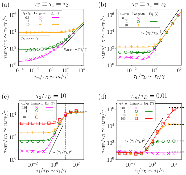
Figure 4: Throughout the figure, colored symbols denote MFPT simulation results and colored lines represent the crossover formula Eq. (7), the barrier height is fixed at $\beta U_{0}=3$. (a), (b) MFPT results for single-exponential memory, i.e., for $\tau_{\Gamma}\equiv\tau_{1}=\tau_{2}$. (a) The rescaled MFPT $\tau_{\mathrm{MFP}}/\tau_{D}$ is shown as a function of the rescaled inertial time $\tau_{m}/\tau_{D}$ for several values of the rescaled memory time $\tau_{\Gamma}/\tau_{D}$. The asymptotic power law scalings $\tau_{\mathrm{MFP}}/\tau_{D}\sim\tau_{m}/\tau_{D}$ (Markovian low-friction regime) and $\tau_{\mathrm{MFP}}/\tau_{D}\equiv$ const. (Markovian high-friction regime) are shown as black bars. (b) The rescaled MFPT $\tau_{\mathrm{MFP}}/\tau_{D}$ is shown as a function of $\tau_{\Gamma}/\tau_{D}$ for several values of $\tau_{m}/\tau_{D}$. The asymptotic power law scaling $\tau_{\mathrm{MFP}}/\tau_{D}\sim(\tau_{\Gamma}/\tau_{D})^{2}$ Straub et al. (1986); Kappler et al. (2018) is shown as a black bar. (c) MFPT results for bi-exponential memory at fixed $\tau_{2}/\tau_{D}=10$ as function of $\tau_{1}/\tau_{D}$ for several fixed values of $\tau_{m}/\tau_{D}$. The value at which $\tau_{1}=\tau_{2}$ is indicated by a vertical dashed line. The black bar indicates the intermediate scaling $\tau_{\mathrm{MFP}}/\tau_{D}\sim(\tau_{1}/\tau_{D})^{2}$, the horizontal dashed black line to the right denotes the prediction from Eq. (7) in the limit $\gamma_{1}=0$. (d) MFPT results for bi-exponential memory at fixed $\tau_{m}/\tau_{D}=0.01$ as function of $\tau_{1}/\tau_{D}$ for several values of $\tau_{2}/\tau_{D}$. The black bar indicates the intermediate scaling $\tau_{\mathrm{MFP}}/\tau_{D}\sim(\tau_{1}/\tau_{D})^{2}$, the horizontal dashed black lines to the right denote the predictions from Eq. (7) in the limit $\gamma_{1}=0$.

IV MFPT results for single-exponential memory and general crossover formula

We first consider the symmetric case $\tau_{\Gamma}\equiv\tau_{1}=\tau_{2}$ where the memory kernel Eq. (3) reduces to a single exponential. For fixed barrier height $\beta U_{0}=3$ one only has two parameters, namely the inertial time $\tau_{m}/\tau_{D}$ and the memory time $\tau_{\Gamma}/\tau_{D}$, both rescaled by the diffusion time. The dependence of the MFPT on $\beta U_{0}$ has previously been considered Kappler et al. (2018), and for the present case is discussed in Appendix G. In Fig. 4 (a) we show MFPTs from simulations for various fixed values of $\tau_{\Gamma}/\tau_{D}$ as a function of $\tau_{m}/\tau_{D}$. As can be most clearly seen for the $\tau_{\Gamma}/\tau_{D}=$ 1 data, for $\tau_{m}/\tau_{D}\ll 1$ the MFPT $\tau_{\mathrm{MFP}}/\tau_{D}$ becomes independent of $\tau_{m}/\tau_{D}$; this is the classical Kramers high-friction regime where $\tau_{\mathrm{MFP}}\sim\gamma$ Kramers (1940); Mel’nikov and Meshkov (1986). In the opposite limit $\tau_{m}/\tau_{D}\gg 1$, the MFPT scales as $\tau_{\mathrm{MFP}}\sim m/\gamma$, indicating the Kramers low-friction (energy diffusion) limit Kramers (1940); Mel’nikov and Meshkov (1986). In Fig. 4 (b) we show simulated MFPTs for various fixed values of $\tau_{m}/\tau_{D}$ as a function of $\tau_{\Gamma}/\tau_{D}$. While for long memory, $(\tau_{\Gamma}/\tau_{D})^{2}\gg\max\{1,\tau_{m}/\tau_{D}\}$, the MFPT scales as $\tau_{\mathrm{MFP}}\sim\tau_{\Gamma}^{2}$ Straub et al. (1986); Kappler et al. (2018), in the Markovian regime $\tau_{\Gamma}/\tau_{D}\ll 1$ the MFPT is independent of $\tau_{\Gamma}/\tau_{D}$. For high friction $\tau_{m}/\tau_{D}\ll 1$, an intermediate regime where memory accelerates barrier crossing compared to the Markovian limit $\tau_{\Gamma}/\tau_{D}\ll 1$, centered around $\tau_{\Gamma}/\tau_{D}\approx 0.1$, can be observed Kappler et al. (2018). We thus see that memory can in the high friction case either accelerate or slow down the barrier-crossing dynamics, depending on the memory time. For long memory the barrier-crossing time grows quadratically with the memory time both for high friction and low friction. This asymptotic regime is intriguing, as it demonstrates that memory modifies the barrier-crossing dynamics, and in particular the mean first-passage time $\tau_{\mathrm{MFP}}$, even when the memory time $\tau_{\Gamma}$ is much shorter than $\tau_{\mathrm{MFP}}$.

We now present a crossover formula for the MFPT for a general multi-exponential memory kernel,

$$\Gamma(t) =\sum_{i=1}^{N}\frac{\gamma_{i}}{\tau_{i}}\exp\left(-{|t|}/{\tau_{i}}\right)$$ (6)

parametrized by friction coefficients $\gamma_{i}$ and memory times $\tau_{i}$, and define the friction coefficient as $\gamma=\sum_{i=1}^{N}\gamma_{i}$. Inspired by the linear dependence of the reaction time on friction in the overdamped limit Kramers (1940) and the linear dependence of the reaction rate on the memory kernel in the energy-diffusion limit Talkner and Braun (1988), we construct a heuristic crossover formula for the MFPT as

$$\tau_{\mathrm{MFP}}=\sum_{i=1}^{n}\tau_{\mathrm{OD}}^{(i)}+\left(\sum_{i=1}^{n}1/\tau_{\mathrm{ED}}^{(i)}\right)^{-1},$$ (7)

where the overdamped MFPT contribution $\tau_{\mathrm{OD}}^{(i)}$ and the energy-diffusion MFPT contribution $\tau_{\mathrm{ED}}^{(i)}$ are given by

$$\frac{\tau_{\mathrm{OD}}^{(i)}}{\tau_{D}} =\frac{\gamma_{i}}{\gamma}\frac{e^{\beta U_{0}}}{\beta U_{0}}\left[\frac{\pi}{2\sqrt{2}}\frac{1}{1+10\beta U_{0}\tau_{i}/\tau_{D}}+\sqrt{\beta U_{0}\frac{\tau_{m}}{\tau_{D}}}~{}\right],$$ (8)

$$\frac{\tau_{\mathrm{ED}}^{(i)}}{\tau_{D}} =\frac{\gamma}{\gamma_{i}}\frac{e^{\beta U_{0}}}{\beta U_{0}}\left[\frac{\tau_{m}}{\tau_{D}}+4\beta U_{0}\left(\frac{\tau_{i}}{\tau_{D}}\right)^{2}+\sqrt{\beta U_{0}\frac{\tau_{m}}{\tau_{D}}}~{}\right].$$ (9)

The first sum in Eq. (7) reflects that in the memoryless high-friction scenario the MFPT scales as $\tau_{\mathrm{MFP}}\sim\gamma=\sum_{i}\gamma_{i}$, as follows from the Kramers theory in the high-friction limit Kramers (1940). The inverse additivity of the individual MFPT contributions in the energy-diffusion regime, the second sum in Eq. (7), is derived in Appendix D. The additivity of the overdamped- and energy-diffusion MFPT contributions in Eq. (7) was previously used to construct similar crossover formulas Hänggi and Weiss (1984); Carmeli and Nitzan (1984); Straub et al. (1985). Our crossover formula for the MFPT obeys an important symmetry: In the case of single-exponential memory, i.e. if all $\tau_{i}$ are equal, Eq. (7) only depends on the $\gamma_{i}$ only via their sum $\gamma$, as it should. In this limit our expression slightly deviates from our previous single-exponential crossover formula Kappler et al. (2018): First, the prefactor $\pi/(2\sqrt{2})\approx 1.11$ in Eq. (8) replaces a factor $1$ in Ref. Kappler et al. (2018), so that Eq. (8) reproduces the overdamped Kramers limit $\tau_{m}/\tau_{D}\ll 1$, $\tau_{\Gamma}/\tau_{D}\ll 1$ Kramers (1940) exactly. Second, the prefactor $4$ in the second term in Eq. (9) replaces a factor $e\approx 2.72$ in Ref. Kappler et al. (2018), which leads to improved matching with simulated MFPTs in the long-memory regime $(\tau_{\Gamma}/\tau_{D})^{2}\gg\max\{1,\tau_{m}/\tau_{D}\}$.

Equation (7) is in Fig. 4 (a), (b) included as colored solid lines and agrees with the numerical data very well. In particular, it reproduces all asymptotic scaling regimes of the single-exponential scenario, namely: i) the memoryless high-friction Kramers regime $\tau_{\Gamma}/\tau_{D}\ll 1$ and $\tau_{m}/\tau_{D}\ll 1$, given by the first term in Eq. (8) for $\tau_{\Gamma}/\tau_{D}=0$ and observed for $\tau_{m}/\tau_{D}\ll 1$ in Fig. 4 (a); ii) the memoryless low-friction regime $\tau_{\Gamma}/\tau_{D}\ll 1$ and $\tau_{m}/\tau_{D}\gg 1$, given by the first term in Eq. (9) and observed for $\tau_{m}/\tau_{D}\gg 1$ in Fig. 4 (a); iii) the long-memory regime $(\tau_{\Gamma}/\tau_{D})^{2}\gg\max\{1,\tau_{m}/\tau_{D}\}$, given by the second term in Eq. (9) and observed for $\tau_{\Gamma}/\tau_{D}\gg 1$ in Fig. 4 (b). The last terms in Eqs. (8) and (9) are included to improve the crossover between the overdamped and energy-diffusion regimes and are fitted to the simulation MFPT data.

In Appendix G, Fig. 11 (a), we compare the crossover formula Eq. (7) with simulation results for varying $\beta U_{0}$ in the symmetric case $\tau_{1}=\tau_{2}$; there, we find good agreement between the crossover formula and numerical results for $\beta U_{0}\gtrsim 2$.

V MFPT results for bi-exponential memory

In Fig. 4 (c), (d) we compare simulation results for $\tau_{\mathrm{MFP}}$ with the crossover formula Eq. (7) for the asymmetric scenario where the bi-exponential memory times $\tau_{1}$ and $\tau_{2}$ are unequal. Figure 4 (c) shows $\tau_{\mathrm{MFP}}/\tau_{D}$ as function of $\tau_{1}/\tau_{D}$ for fixed $\tau_{2}/\tau_{D}=10$ and several values of $\tau_{m}/\tau_{D}$. Throughout Fig. 4 (c) the crossover formula Eq. (7), denoted by colored solid lines, describes the simulation results very well. We see that for $\tau_{1}\ll\tau_{2}$, i.e. to the left of the vertical dashed line that denotes $\tau_{1}=\tau_{2}$, the MFPT behaves very similarly to the single-exponential MFPT results shown in Fig. 4 (b). As $\tau_{1}\gtrsim\tau_{2}$, i.e. to the right of the vertical dashed line, the MFPT becomes independent of $\tau_{1}$ and takes on the value which is obtained in the absence of the more slowly decaying exponential memory component, as indicated by the horizontal dashed black line which follows from Eq. (7) by taking the limit $\gamma_{1}=0$. In agreement with the behavior of the particle trajectories and the FPT distributions discussed before, the MFPT only depends on the shorter of the two memory times if at least one of the two memory times $\tau_{1}$, $\tau_{2}$ is larger than $\tau_{D}$.

Figure 4 (d) shows $\tau_{\mathrm{MFP}}/\tau_{D}$ as function of $\tau_{1}/\tau_{D}$ for fixed $\tau_{m}/\tau_{D}=10$ and several values of $\tau_{2}/\tau_{D}$ as indicated in the legend. Also in this plot, the crossover formula Eq. (7) describes the simulation data very accurately. For $\tau_{1}\ll\tau_{2}$ we again obtain behavior reminiscent of the single-exponential results shown in Fig. 4 (b). As $\tau_{1}\gtrsim\tau_{2}$ and $\tau_{1}>\tau_{D}$, $\tau_{\mathrm{MFP}}/\tau_{D}$ saturates at a value that only depends on $\tau_{m}/\tau_{D}$ and $\tau_{2}/\tau_{D}$, while the value of $\tau_{1}$ becomes irrelevant. The horizontal dashed black lines to the right of the figure denote the predictions from Eq. (7) in the limit $\gamma_{1}=0$. For $\tau_{2}/\tau_{D}=0.01$ (magenta crosses), Fig. 4 (d) contains no regime where $\tau_{D}<\tau_{1}\ll\tau_{2}$, so that $\tau_{\mathrm{MFP}}$ is almost independent of $\tau_{1}/\tau_{D}$ throughout.

In Appendix F we compare our crossover formula to simulation data for a wider range of the parameters $\tau_{m}/\tau_{D}$, $\tau_{1}/\tau_{D}$, $\tau_{2}/\tau_{D}$ at barrier height $\beta U_{0}=3$, confirming that Eq. (7) globally describes bi-exponential barrier crossing very well and that $\tau_{\mathrm{MFP}}$ is dominated by the shorter memory time for all parameter values. In Appendix G we show that our crossover formula Eq. (7) agrees with simulations also for larger barrier heights $\beta U_{0}$. As demonstrated in Appendix E, Grote-Hynes (GH) theory Grote and Hynes (1980) only describes the simulation data in the triple-limit of high-friction $\tau_{m}/\tau_{D}\ll 1$ and short memory $\tau_{1}/\tau_{D}\ll 1$, $\tau_{2}/\tau_{D}\ll 1$, which is why we do not compare our results with predictions of GH theory in the main text.

The dependence of the MFPT on the memory times $\tau_{1}$ and $\tau_{2}$ is summarized in Fig. 5 in terms of scaling diagrams for both high and low friction. For high friction, $\tau_{m}/\tau_{D}=0.01$, we see in Fig. 5 (a) that the Markovian high-friction regime, which corresponds to the Kramers high-friction regime where $\tau_{\mathrm{MFP}}\sim\gamma$ Kramers (1940), is obtained when both $\tau_{1}/\tau_{D}$ and $\tau_{2}/\tau_{D}$ become small. For $\tau_{1}/\tau_{D}>1$ and $\tau_{2}/\tau_{D}>1$ the memory slowdown regime is reached where the MFPT increases quadratically with the memory time. This regime is divided along the diagonal, since the shorter memory time dominates the barrier-crossing kinetics, such that for $\tau_{1}>\tau_{2}$ one finds $\tau_{\mathrm{MFP}}\sim\tau_{2}^{2}$ while for $\tau_{1}<\tau_{2}$ one finds $\tau_{\mathrm{MFP}}\sim\tau_{1}^{2}$. The Markovian and memory slowdown asymptotic regimes are separated by an intermediate memory speedup regime, where barrier crossing is slightly accelerated by the presence of memory as compared to the Markovian limit. Along the diagonal $\tau_{1}=\tau_{2}$, the intermediate memory speedup and the asymptotic memory slowdown regimes are illustrated in Fig. 4 (b); parallel to the $\tau_{1}$-axis, the memory speedup is illustrated in Fig. 5 (c) by a plot of $\tau_{\mathrm{MFP}}$ for constant $\tau_{2}/\tau_{D}=10^{-4}$.

For low friction, $\tau_{m}/\tau_{D}=10$, shown in Fig. 5 (b), the Markovian regime is obtained for $\tau_{1}/\tau_{D}<1$ and $\tau_{2}/\tau_{D}<1$. For $\tau_{1}/\tau_{D}\gg\max\{1,\sqrt{\tau_{m}/\tau_{D}}\}=\sqrt{10}$ and $\tau_{2}/\tau_{D}\gg\max\{1,\sqrt{\tau_{m}/\tau_{D}}\}=\sqrt{10}$ the memory slowdown regime is reached where $\tau_{\mathrm{MFP}}\sim\tau_{2}^{2}$ or $\tau_{\mathrm{MFP}}\sim\tau_{1}^{2}$, depending on which memory time is smaller. In between these two asymptotic regimes, we find an intermediate regime where the barrier crossing is slowed down compared to the Markovian limit but the MFPT does not display the quadratic memory-time dependence, which is illustrated in Fig. 5 (d) by a plot of $\tau_{\mathrm{MFP}}$ for constant $\tau_{2}/\tau_{D}=10^{-4}$. A plot of $\tau_{\mathrm{MFP}}$ along the diagonal for $\tau_{1}=\tau_{2}$ is shown in Fig. 4 (b).

There are different levels on which one can rationalize and intuitively understand the main result obtained here, namely that it is the memory contribution with the shorter decay time that dominates the barrier-crossing kinetics in the non-Markovian limit. On a formal level, the linear pole analysis of the positional autocorrelation function in Appendix C shows that for $\tau_{D}<\tau_{1}\ll\tau_{2}$, the memory contribution that depends on $\tau_{2}$ can be neglected, so that the particle motion only depends on $\tau_{1}$.

An alternative viewpoint is obtained by mapping of the non-Markovian one-dimensional Langevin equation onto a system of $N$ coupled Markovian degrees of freedom, see Appendix B. In this picture, each exponential contribution to the memory function $\Gamma(t)$ can be viewed as an independent heat bath with relaxation time $\tau_{i}$, with which the particle exchanges energy, see Appendix B. Accordingly, the inverse additivity of the MFPTs of each exponential memory contribution in the energy-diffusion regime, represented by the second term in Eq. (7), means that $\tau_{\mathrm{MFP}}$ is dominated by the heat bath with the shortest relaxation time, i.e. by the heat bath which is the fastest in providing the particle with the energy needed for barrier crossing, which (for identical $\gamma_{i}$) is the heat bath with the smallest $\tau_{i}$. In conclusion, for bi-exponential memory, the shorter of the two memory times dominates the barrier-crossing time simply because it provides the barrier-crossing energy faster.

Yet another way of understanding the dominance of the memory contribution with the shorter decay time is obtained by considering the memory integral in Eq. (1) for a bi-exponential kernel given by Eq. (3). The particle will undergo many oscillations (for low friction) or random fluctuations (for high friction) within a well before attempting to cross the barrier. If the memory times are longer than the intrinsic relaxation time of the particle (which can be the intrinsic diffusion time $\tau_{D}$ or the oscillation period depending on whether one is in the high-friction or the low-friction regime), the convolution of the particle velocity history with the exponential memory contribution with the longer memory time will give a smaller friction contribution than the convolution with the exponential memory contribution with the shorter memory time (again assuming equal memory amplitudes $\gamma_{1}$ and $\gamma_{2}$), simply because the mean of the particle velocity is zero. This shows directly that memory effects in confinement tend to be dominated by the shorter memory contributions.

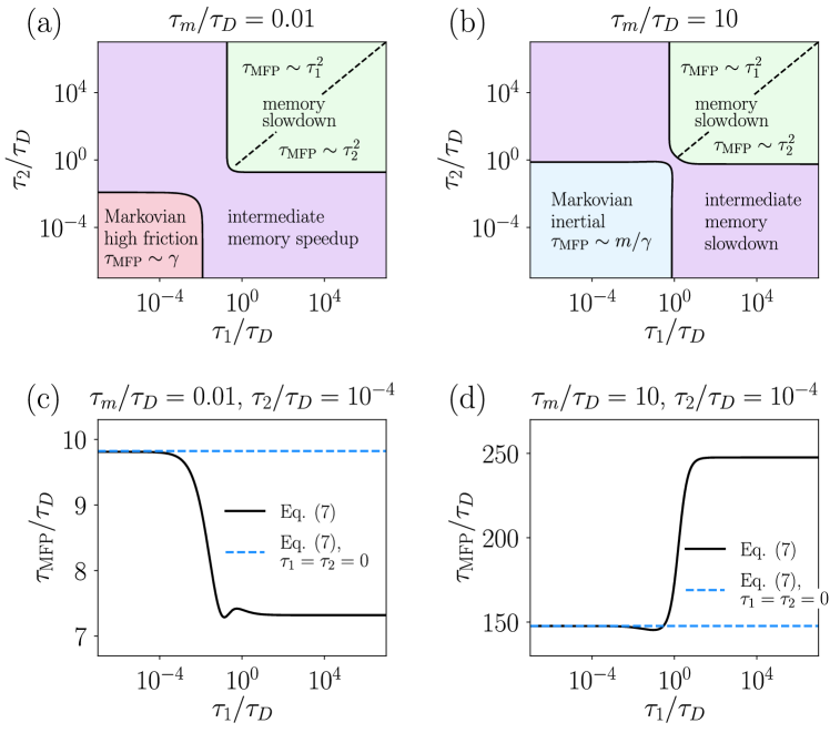
Figure 5: (a), (b) Scaling diagrams for the dependence of the MFPT $\tau_{\mathrm{MFP}}$ on the rescaled memory times $\tau_{1}/\tau_{D}$ and $\tau_{2}/\tau_{D}$ for (a) high friction $\tau_{m}/\tau_{D}=0.01$ and (b) low friction $\tau_{m}/\tau_{D}=10$. In (a), the transition from the Markovian high-friction regime to the intermediate memory speedup regime is defined by the location where $\tau_{\mathrm{MFP}}$ is smaller by 10% than the Markovian limit $\tau_{1}=\tau_{2}=0$ (based on the crossover formula Eq. (7)). The transition from the intermediate memory speedup regime to the asymptotic memory slowdown regime is defined by the location where $\tau_{\mathrm{MFP}}$ equals the Markovian limit. In (b), the transition from the Markovian low-friction regime to the intermediate memory slowdown regime is defined by the location where $\tau_{\mathrm{MFP}}$ is larger by 10% than the Markovian limit $\tau_{1}=\tau_{2}=0$ (based on the crossover formula Eq. (7)). The transition from the intermediate memory slowdown regime to the asymptotic memory slowdown regime is defined by the location where $\tau_{\mathrm{MFP}}$ is twice as large as in the Markovian limit. The dashed diagonal lines in (a) and (b) in the asymptotic memory slowdown regime indicate the crossover from $\tau_{1}$-dominated barrier crossing for $\tau_{1}\ll\tau_{2}$, to $\tau_{2}$-dominated barrier crossing for $\tau_{2}\ll\tau_{1}$. (c), (d) The rescaled MFPT $\tau_{\mathrm{MFP}}/\tau_{D}$ according to Eq. (7) is shown as a function of $\tau_{1}/\tau_{D}$ for fixed $\tau_{2}/\tau_{D}=10^{-4}$ and (a) $\tau_{m}/\tau_{D}=0.01$, and (b) $\tau_{m}/\tau_{D}=10$. The dashed line denotes the Markovian limit, obtained from Eq. (7) by setting $\tau_{1}=\tau_{2}=0$. All data is obtained for a fixed barrier height of $\beta U_{0}=3$.

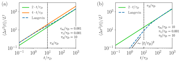
Figure 6: Comparison of the simulated mean-squared displacement (MSD), shown as dashed blue line (consisting of 8 data points per decade), with asymptotic predictions in the absence of an external potential for $U(x)=0$. (a) Results for high friction $\tau_{m}/\tau_{D}=0.001$ and memory times $\tau_{1}/\tau_{D}=0.001$ and $\tau_{2}/\tau_{D}=10$, the same parameters as used in Fig. 2 (c). The solid lines denote the expected MSD for diffusion with friction coefficients $\gamma/2$ (orange line) and $\gamma$ (green line). The vertical dashed line denotes $\tau_{2}/\tau_{D}$. (b) Results for low friction $\tau_{m}/\tau_{D}=10$ and memory times $\tau_{1}/\tau_{D}=0.001$ and $\tau_{2}/\tau_{D}=10$, the same parameters as used in Fig. 2 (f). The solid green line denotes the expected MSD for diffusion with friction coefficient $\gamma$. The black bar indicates the power law $\langle\Delta x^{2}(t)\rangle\sim t^{2}$ expected for ballistic motion, the vertical dashed line denotes $\tau_{2}/\tau_{D}$. Note that for free diffusion there exist analytical expressions for both the Laplace- and Fourier-transform of the MSD Grabert et al. (1988); Kappler et al. (2019), so that Fig. 6 could have been generated without invoking numerical simulations.

VI Free diffusion case

While barrier-crossing dynamics is dominated by the memory contribution with the shorter memory time in the non-Markovian limit, in the absence of an external potential, i.e. for $U(x)=0$, the long-time diffusive behavior is always expected to be determined by the total friction $\gamma=\gamma_{1}+\gamma_{2}$. In Fig. 6 we show mean-squared displacements (MSDs)

$$\langle\Delta x^{2}(t)\rangle=\left\langle\left[x(t)-x(0)\right]^{2}\right\rangle$$ (10)

obtained from simulations without an external potential, $U(x)=0$, and unequal memory times $\tau_{1}/\tau_{D}=0.001$, $\tau_{2}/\tau_{D}=10$, as blue dashed lines. These parameters used are the same as in Fig. 2 (c), (f). Figure 6 (a) shows the high-friction scenario $\tau_{m}/\tau_{D}=0.001$. For times $t\gg\tau_{2}$ the MSD is well described by

$$\langle\Delta x^{2}(t)\rangle=2\frac{1}{\beta\gamma}t=2Dt,$$ (11)

which in Fig. 6 (a) is denoted by a green solid line, and which is the expected result for the MSD of a Brownian particle with friction coefficient $\gamma$ and where we used the Einstein relation to define the diffusion constant as $D=1/(\beta\gamma)$. For shorter times $\tau_{1}<t<\tau_{2}$, only the shorter memory contribution, characterized by $\tau_{1}$, contributes to the friction and the simulated MSD is well described by

$$\langle\Delta x^{2}(t)\rangle=2\frac{1}{\beta\gamma_{1}}t=4Dt,$$ (12)

which in Fig. 6 (a) is denoted by an orange solid line.

For the low-friction scenario $\tau_{m}/\tau_{D}=10$ depicted in Fig. 6 (b), the inertial regime where $\langle\Delta x^{2}(t)\rangle\sim t^{2}/(m\beta)$ appears for $t\ll\tau_{m}$. For $t\gtrsim\tau_{m}$ the MSD exhibits diffusive behavior determined by the full friction coefficient $\gamma$, i.e. $\langle\Delta x^{2}(t)\rangle=2t/(\beta\gamma)=2Dt$, since for $t\gg\tau_{m}$ we simultaneously fulfill $t\gg\tau_{1}$ and $t\gg\tau_{2}$.

We conclude that while barrier-crossing kinetics is completely dominated by the shorter memory time if the particle relaxation time is shorter than the longer memory time, the long-time free diffusion behavior in the presence of bi-exponential memory is determined by the sum of both exponential memory contributions. This simply reflects that the particle relaxation time diverges in the free-diffusion scenario.

VII Conclusions

Our Langevin simulations in the presence of a bi-exponential memory function show that if at least one of the two memory times $\tau_{1}$, $\tau_{2}$ is larger than $\tau_{D}$, then the barrier-crossing time $\tau_{\mathrm{MFP}}$ is dominated by the shorter of the two memory times. The simulation results are obtained for the restricted case where the exponential memory contributions have the same integral weight. Based on asymptotic matching and symmetry considerations, we construct a crossover formula for $\tau_{\mathrm{MFP}}$ which describes our simulation results for all parameters very well. This formula applies to general multi-exponential memory function with arbitrary weights and decay times and corroborates that the shortest memory time is expected to dominate $\tau_{\mathrm{MFP}}$ in the non-Markovian limit.

Our results have a number of important consequences: Usually it is assumed that the slow degrees of freedom of a system dominate rare events and in particular the MFPT $\tau_{\mathrm{MFP}}$; for the case of barrier crossing in the presence of memory functions with different time scales, our results show that this time scale separation principle is violated. Our findings suggest that instead of keeping only the slowest degrees of freedom, which is conventionally done in coarse graining procedures, one also needs to keep the fastest orthogonal degrees of freedom if non-Markovian effects are important. Of course, the choice of the degrees of freedom that should be included requires good understanding of all relevant time scales.

Non-Markovian effects have been demonstrated to be important for fast molecular transition such as the dihedral barrier dynamics of butane in solvents de Sancho et al. (2014); Daldrop et al. (2018a). The effect of the different memory times of the multi-scale memory kernel that have been extracted from simulations will have to be examined in future work. Likewise, protein dynamics has been suggested to be subject to memory effects in a number of works Plotkin and Wolynes (1998); Das and Makarov (2018). Here our crossover formula Eq. (7) will be useful, because it fills the gap between theoretical works on non-Markovian barrier crossing, which are typically confined to single-exponential memory Straub et al. (1986); Pollak et al. (1989); Ianconescu and Pollak (2015), and real physical systems, where orthogonal degrees of freedom typically feature several relaxation time scales Rey and Guardia (1992); Tolokh et al. (2002); de Sancho et al. (2014); Lesnicki et al. (2016); Gottwald et al. (2015); Daldrop et al. (2017, 2018a). Another field of application are chemical reactions in solvents, such as proton transfer reactions in water Marx et al. (1999); Marx (2006). In such reactions, the friction is presumably rather small, such that the low-friction regime, characterized by $\tau_{m}/\tau_{D}>1$, is relevant. But also in the low-friction limit, our results show that for multi-scale memory the smaller memory time becomes dominant in the non-Markovian limit.

Appendix A Dimensionless form of the GLE

We consider the one-dimensional generalized Langevin equation

$$m\,\ddot{x}(t)=-\int_{0}^{t}\Gamma(t-t^{\prime})\dot{x}(t^{\prime})\,\mathrm{d}t^{\prime}-U^{\prime}(x(t))+\eta(t),$$ (13)

where $m$ is the mass of the particle, $x$ its position, $\Gamma(t)$ the memory kernel and $U^{\prime}(x)$ denotes the derivative of the external potential $U(x)$. The random force $\eta(t)$ is Gaussian with zero mean, $\langle\eta(t)\rangle=0$, and obeys the generalized fluctuation-dissipation theorem (FDT)

$$\beta\langle\eta(t)\eta(t^{\prime})\rangle =\Gamma(|t-t^{\prime}|).$$ (14)

We consider a multi-exponential memory kernel with friction coefficients $\gamma_{i}$ and memory times $\tau_{i}$,

$$\Gamma(t)=\sum_{i=1}^{N}\frac{\gamma_{i}}{\tau_{i}}e^{-|t|/\tau_{i}},$$ (15)

and define the total friction $\gamma:=\sum_{i=1}^{N}\gamma_{i}$. Defining a dimensionless position $\tilde{x}=x/L$ and a rescaled time $t=\tilde{t}\tau_{D}$ and multiplying Eq. (13) by $\beta L$, we obtain

$$\frac{\tau_{m}}{\tau_{D}}\ddot{\tilde{x}}(\tilde{t})=-\sum_{i=1}^{N}\frac{\gamma_{i}}{\gamma}\frac{\tau_{D}}{\tau_{i}}\int_{0}^{\tilde{t}}\mathrm{d}\tilde{t}^{\prime}\exp\left[-\frac{\tau_{D}}{\tau_{i}}\left(\tilde{t}-\tilde{t}^{\prime}\right)\right]\dot{\tilde{x}}(\tilde{t}^{\prime})+\tilde{F}\left(\tilde{x}(\tilde{t}\,)\right)+\tilde{\eta}(\tilde{t}),$$ (16)

where $\tilde{F}(\tilde{x}):=\beta L\partial_{x}U(L\tilde{x})\equiv\beta LU^{\prime}(L\tilde{x})$ and $\tilde{\eta}(\tilde{t}):=\beta L\,\eta(\tau_{D}\tilde{t})$. Using Eq. (14), it follows that the autocorrelation of the dimensionless random force is given by

$$\left\langle\tilde{\eta}(\tilde{t})\tilde{\eta}(\tilde{t}^{\prime})\right\rangle=\sum_{i=1}^{N}\frac{\gamma_{i}}{\gamma}\frac{\tau_{D}}{\tau_{i}}\exp\left[-\frac{\tau_{D}}{\tau_{i}}|\tilde{t}-\tilde{t}^{\prime}|\right].$$ (17)

For $N=1$ we recover the case of single-exponential memory, for $N=2$ and $\gamma_{1}=\gamma_{2}$ we obtain the symmetric bi-exponential system that we considered in the simulations. For given potential $U$, Eqs. (16), (17), are fully determined by the dimensionless ratios $\tau_{m}/\tau_{D}$, $\tau_{i}/\tau_{D}$, $\gamma_{i}/\gamma$.

Appendix B Transforming the GLE into a coupled system of Markovian equations

We now show that the dimensionless GLE with multi-exponential memory, Eqs. (16), (17), is equivalent to the Markovian coupled system of equations

$$m\ddot{x} =-\partial_{x}V,$$ (18)

$$0 =-\gamma_{i}\dot{y}_{i}-\partial_{i}V+\xi_{i},\qquad i\in\{1,...,N\},$$ (19)

where the $\xi_{i}$ are Markovian Gaussian random fields with zero mean and variance

$$\beta\left\langle\xi_{i}(t)\xi_{j}(t)\right\rangle=2\gamma_{i}\delta_{i,j}\delta(t-t^{\prime}),\qquad i,j\in\{1,...,N\},$$ (20)

the potential $V$ is given by

$$V(x,y_{1},...,y_{N})=U(x)+\sum_{j=1}^{N}\frac{k_{j}}{2}(y_{j}-x)^{2},$$ (21)

and $\partial_{i}V$ denotes the partial derivative of $V$ w.r.t. $y_{i}$.

Defining dimensionless positions $\tilde{x}(\tilde{t}):=x(\tau_{D}\tilde{t})/L$, $\tilde{y}_{i}(\tilde{t}):=y_{i}(\tau_{D}\tilde{t})/L$, inserting the potential Eq. (21) in Eqs. (18), (19), introducing a rescaled time variable $t=\tilde{t}\tau_{D}$, and multiplying by $\beta L$, we obtain

$$\frac{\tau_{m}}{\tau_{D}}\ddot{\tilde{x}}(\tilde{t}\,) =\tilde{F}\left(\tilde{x}(\tilde{t}\,)\right)+\sum_{i=1}^{N}\frac{\tau_{D}}{\tau_{i}}\frac{\gamma_{i}}{\gamma}\left[\tilde{y}_{i}(\tilde{t})-\tilde{x}(\tilde{t}\,)\right],$$ (22)

$$\dot{\tilde{y}}_{i}(\tilde{t}\,) =-\frac{\tau_{D}}{\tau_{i}}\tilde{y}_{i}(\tilde{t}\,)+\frac{\tau_{D}}{\tau_{i}}\tilde{x}(\tilde{t}\,)+\sqrt{\frac{\gamma}{\gamma_{i}}}\tilde{\xi}_{i}(\tilde{t}\,)\quad 1\leq i\leq N,$$ (23)

where $\tilde{F}(\tilde{x}):=-\beta L\partial_{x}U(L\tilde{x})\equiv\beta LU^{\prime}(L\tilde{x})$, $\tau_{i}:=\gamma_{i}/k_{i}$, and the correlators of the dimensionless random forces $\tilde{\xi}(\tilde{t}):=\beta L\,\sqrt{\gamma/\gamma_{i}}\xi(\tau_{D}\tilde{t})$ are given by

$$\left\langle\tilde{\xi}_{i}(\tilde{t}\,)\tilde{\xi}_{j}(\tilde{t}\,)\right\rangle=2\delta_{i,j}\delta(\tilde{t}-\tilde{t}^{\prime})\qquad i,j\in\{1,...,N\}.$$ (24)

To show the equivalence of Eqs. (22), (23), (24) to the GLE Eq. (16), (17), we first note that the solution to Eq. (23) is given by

$$\tilde{y}_{i}(\tilde{t}\,) =\tilde{y}_{i}(0)\exp\left(-\frac{\tau_{D}}{\tau_{i}}\tilde{t}\right)$$

$$\qquad+\frac{\tau_{D}}{\tau_{i}}\int_{0}^{\tilde{t}}\mathrm{d}\tilde{t}^{\prime}\exp\left[-\frac{\tau_{D}}{\tau_{i}}(\tilde{t}-\tilde{t}^{\prime})\right]\tilde{x}(\tilde{t}^{\prime})$$ (25)

$$\qquad+\sqrt{\frac{\gamma}{\gamma_{i}}}\int_{0}^{\tilde{t}}\mathrm{d}\tilde{t}^{\prime}\exp\left[-\frac{\tau_{D}}{\tau_{i}}(\tilde{t}-\tilde{t}^{\prime})\right]\tilde{\xi}_{i}(\tilde{t}^{\prime}).$$

Using integration by parts on the second term of this expression and inserting the result into Eq. (22), we obtain

$$\frac{\tau_{m}}{\tau_{D}}\ddot{\tilde{x}}(\tilde{t}) =-\sum_{i=1}^{N}\frac{\gamma_{i}}{\gamma}\frac{\tau_{D}}{\tau_{i}}\int_{0}^{\tilde{t}}\mathrm{d}\tilde{t}^{\prime}\exp\left[-\frac{\tau_{D}}{\tau_{i}}\left(\tilde{t}-\tilde{t}^{\prime}\right)\right]\dot{\tilde{x}}(\tilde{t}^{\prime})+\tilde{F}(\tilde{x}(\tilde{t}))+\tilde{\eta}_{R}(\tilde{t}),$$ (26)

where we define

$$\tilde{\eta}_{R}(\tilde{t}) =\sum_{i=1}^{N}\left\{\frac{\gamma_{i}}{\gamma}\frac{\tau_{D}}{\tau_{i}}\left[\tilde{y}_{i}(0)-\tilde{x}(0)\right]\exp\left[-\frac{\tau_{D}}{\tau_{i}}\left(\tilde{t}\,\right)\right]\vphantom{+\sqrt{\frac{\gamma_{i}}{\gamma}}\frac{\tau_{D}}{\tau_{i}}\int_{0}^{\tilde{t}}\mathrm{d}\tilde{t}^{\prime}\exp\left[-\frac{\tau_{D}}{\tau_{i}}(\tilde{t}-\tilde{t}^{\prime})\right]\tilde{\xi}_{i}(\tilde{t}^{\prime})}\right.$$ (27)

$$\qquad\left.+\sqrt{\frac{\gamma_{i}}{\gamma}}\frac{\tau_{D}}{\tau_{i}}\int_{0}^{\tilde{t}}\mathrm{d}\tilde{t}^{\prime}\exp\left[-\frac{\tau_{D}}{\tau_{i}}(\tilde{t}-\tilde{t}^{\prime})\right]\tilde{\xi}_{i}(\tilde{t}^{\prime})\right\}.$$

To obtain the equivalence of Eq. (26) to Eq. (16), $\tilde{\eta}_{R}$ needs to be a stochastic processes identical to $\tilde{\eta}$. For this, we assume that, for given $x(0)$, the $y_{i}(0)$ are distributed according to a Boltzmann distribution $\rho(y_{1}(0),...,y_{N}(0)\,|\,x(0))\sim\exp\left[-\beta V(x(0),y_{1}(0),...,y_{N}(0))\right]$, which using Eq. (21) leads to normally distributed $\tilde{y}_{i}(0)-\tilde{x}(0)$ with zero mean and covariance matrix

$$\left\langle\left[\tilde{y}_{i}(0)-\tilde{x}(0)\right]\left[\tilde{y}_{j}(0)-\tilde{x}(0)\right]\right\rangle=\delta_{i,j}\left(\frac{\gamma_{i}}{\gamma}\frac{\tau_{D}}{\tau_{i}}\right)^{-1}.$$ (28)

With this, the mean of $\tilde{\eta}_{R}$ is easily seen to be zero, and the variance is given by

$$\left\langle\tilde{\eta}_{R}(\tilde{t})\tilde{\eta}_{R}(\tilde{t}^{\prime})\right\rangle =\sum_{i=1}^{N}\left(\frac{\gamma_{i}}{\gamma}\frac{\tau_{D}}{\tau_{i}}\right)^{2}\exp\left[-\frac{\tau_{D}}{\tau_{i}}(\tilde{t}+\tilde{t}^{\prime})\right]\left\langle\left(\tilde{y}_{i}(0)-\tilde{x}(0)\right)^{2}\right\rangle$$ (29)

$$\quad+\sum_{i=1}^{N}\frac{\gamma_{i}}{\gamma}\left(\frac{\tau_{D}}{\tau_{i}}\right)^{2}\int_{0}^{\tilde{t}}\mathrm{d}u\int_{0}^{\tilde{t}^{\prime}}\mathrm{d}u^{\prime}\,\exp\left[-\frac{\tau_{D}}{\tau_{i}}(\tilde{t}+\tilde{t}^{\prime}-u-u^{\prime})\right]\langle\tilde{\xi}_{i}(u)\tilde{\xi}_{i}(u^{\prime})\rangle$$

$$=\sum_{i=1}^{N}\exp\left[-\frac{\tau_{D}}{\tau_{i}}(\tilde{t}+\tilde{t}^{\prime})\right]\frac{\gamma_{i}}{\gamma}\frac{\tau_{D}}{\tau_{i}}$$

$$\quad+\sum_{i=1}^{N}2\frac{\gamma_{i}}{\gamma}\left(\frac{\tau_{D}}{\tau_{i}}\right)^{2}\int_{0}^{\min\{\tilde{t},\tilde{t}^{\prime}\}}\mathrm{d}u\,\exp\left[-\frac{\tau_{D}}{\tau_{i}}(\tilde{t}+\tilde{t}^{\prime}-2u)\right]$$ (30)

$$=\sum_{i=1}^{N}\exp\left[-\frac{\tau_{D}}{\tau_{i}}(\tilde{t}+\tilde{t}^{\prime})\right]\frac{\gamma_{i}}{\gamma}\frac{\tau_{D}}{\tau_{i}}$$

$$\quad+\sum_{i=1}^{N}\frac{\gamma_{i}}{\gamma}\frac{\tau_{D}}{\tau_{i}}\left\{\exp\left[-\frac{\tau_{D}}{\tau_{i}}\left(\tilde{t}+\tilde{t}^{\prime}-2\min\{\tilde{t},\tilde{t}^{\prime}\}\right)\right]-\exp\left[-\frac{\tau_{D}}{\tau_{i}}\left(\tilde{t}+\tilde{t}^{\prime}\right)\right]\right\}$$ (31)

$$=\sum_{i=1}^{N}\frac{\gamma_{i}}{\gamma}\frac{\tau_{D}}{\tau_{i}}\exp\left[-\frac{\tau_{D}}{\tau_{i}}|\tilde{t}-\tilde{t}^{\prime}|\right],$$ (32)

where we use that $\tilde{t}+\tilde{t}^{\prime}-2\min\{\tilde{t},\tilde{t}^{\prime}\}=|\tilde{t}-\tilde{t}^{\prime}|$. Thus, $\tilde{\eta}_{R}$ is a Gaussian stochastic process with the first two moments identical to those of the Gaussian stochastic process $\tilde{\eta}$, so that $\tilde{\eta}_{R}\equiv\tilde{\eta}$. For $N=2$ and $\gamma_{1}=\gamma_{2}$, we obtain the system considered in the simulations in the main text.

To simulate Eqs. (22), (23) using a Runge-Kutta scheme, we introduce a further auxiliary variable $z$ to rewrite the equations as a system of first-order equations

$$\dot{\tilde{x}}(\tilde{t}\,) =z(\tilde{t}\,),$$ (33)

$$\frac{\tau_{m}}{\tau_{D}}\dot{z}(\tilde{t}\,) =\sum_{i=1}^{N}\frac{\tau_{D}}{\tau_{i}}\frac{\gamma_{i}}{\gamma}\left[\tilde{y}_{j}(\tilde{t})-\tilde{x}(\tilde{t}\,)\right]+\tilde{F}\left(\tilde{x}(\tilde{t}\,)\right),$$ (34)

$$\dot{\tilde{y}}_{i}(\tilde{t}\,) =-\frac{\tau_{D}}{\tau_{i}}\left[\tilde{y}_{i}(\tilde{t}\,)-\tilde{x}(\tilde{t}\,)\right]+\sqrt{\frac{\gamma}{\gamma_{i}}}\tilde{\xi}_{i}(\tilde{t}\,)\quad 1\leq i\leq N,$$ (35)

Note that the equivalence of Eqs. (18), (19), (20), (21) to Eqs. (16), (17), physically means that multi-exponential memory can be interpreted as the result of the interaction of a particle $x$ with $N$ independent reservoirs $y_{i}$ with finite relaxation times $\tau_{i}$.

Appendix C Analysis of autocorrelation function

In Fig. 2 we observe similarities between the dynamics in the asymmetric bi-exponential scenario $\tau_{1}\ll\tau_{2}$ and the single-exponential scenario characterized by the smaller memory time $\tau_{1}$, indicating that the smaller memory time dominates the barrier-crossing kinetics. This can be rationalized by an asymptotic analysis of the autocorrelation function $C(t)\equiv\langle x(t)x(0)\rangle$ that characterizes the particle motion within one potential well. The following calculation is a generalization of the analysis carried out for the single-exponential memory kernel in Ref. Kappler et al. (2018). We consider the GLE (1) in a harmonic potential $U(x)\simeq Kx^{2}/2$ and for times $t\gg\tau_{1},\tau_{2}$, so that we can replace the upper limit in the memory integral by infinity. Fourier transforming Eq. (1) and solving for $\tilde{x}(\omega)$ yields

$$\tilde{x}(\omega) =\frac{\tilde{\eta}(\omega)}{K-m\omega^{2}+i\omega\tilde{\Gamma}_{+}(\omega)}\equiv\tilde{Q}(\omega)\tilde{\eta}(\omega),$$ (36)

where the half-sided Fourier transform $\tilde{\Gamma}_{+}$ of the bi-exponential memory kernel $\Gamma(t)$ is given by

$$\tilde{\Gamma}_{+}(\omega) =\int_{0}^{\infty}\mathrm{d}t~{}e^{-i\omega t}\Gamma(t)=\frac{\gamma}{2}\sum_{j=1}^{2}\frac{1}{1+i\omega\tau_{j}},$$ (37)

while the full Fourier transform is

$$\tilde{\Gamma}(\omega) =\tilde{\Gamma}_{+}(\omega)+\tilde{\Gamma}_{+}(-\omega)=\gamma\sum_{j=1}^{2}\frac{1}{1+\omega^{2}\tau_{j}^{2}}.$$ (38)

Using Eq. (36), we calculate the autocorrelation function $C(t)\equiv\langle x(t)x(0)\rangle$ as

$$C(t) \equiv\langle x(t)x(0)\rangle=\int\frac{\mathrm{d}\omega}{2\pi}e^{i\omega t}~{}\int\frac{\mathrm{d}\omega^{\prime}}{2\pi}~{}\langle\tilde{x}(\omega)\tilde{x}(\omega^{\prime})\rangle$$ (39)

$$=\int\frac{\mathrm{d}\omega}{2\pi}e^{i\omega t}~{}\int\frac{\mathrm{d}\omega^{\prime}}{2\pi}~{}\tilde{Q}(\omega)\tilde{Q}(\omega^{\prime})\langle\tilde{\eta}(\omega)\tilde{\eta}(\omega^{\prime})\rangle$$ (40)

$$=\beta^{-1}\int\frac{\mathrm{d}\omega}{2\pi}e^{i\omega t}~{}\int\frac{\mathrm{d}\omega^{\prime}}{2\pi}~{}2\pi\delta(\omega+\omega^{\prime})\tilde{\Gamma}(\omega)\tilde{Q}(\omega)\tilde{Q}(\omega^{\prime})$$ (41)

$$=\beta^{-1}\int\frac{\mathrm{d}\omega}{2\pi}e^{i\omega t}~{}\tilde{\Gamma}(\omega)\tilde{Q}(\omega)\tilde{Q}(-\omega),$$ (42)

where we used that the Fourier transform of the generalized FDT is $\langle\tilde{\eta}(\omega)\tilde{\eta}(\omega^{\prime})\rangle=\beta^{-1}~{}2\pi\delta(\omega+\omega^{\prime})~{}\tilde{\Gamma}(\omega)$. Thus the Fourier transform of $C(t)$ is finally given by

$$\beta\tilde{C}(\omega) =\tilde{\Gamma}(\omega)\tilde{Q}(\omega)\tilde{Q}(-\omega)$$ (43)

$$=\gamma\sum_{j=1}^{2}\left[\frac{1}{1+\omega^{2}\tau_{j}^{2}}\frac{1}{K-m\omega^{2}+i\omega\gamma/2\sum_{k=1}^{2}(1+i\omega\tau_{k})^{-1}}\right.$$

$$\hskip 85.35826pt\left.\times\frac{1}{K-m\omega^{2}-i\omega\gamma/2\sum_{l=1}^{2}(1-i\omega\tau_{l})^{-1}}\right]$$ (44)

$$=\gamma\sum_{j=1}^{2}\left\{(1+\omega^{2}\tau_{j}^{2})\left[(K-m\omega^{2})^{2}-\omega\gamma\sum_{k=1}^{2}\omega\tau_{k}(1+\omega^{2}\tau_{k}^{2})^{-1}\right.\right.$$ (45)

$$\hskip 113.81102pt\left.\left.+\frac{\omega^{2}\gamma^{2}}{4}\sum_{k,l=1}^{2}(1+i\omega\tau_{k})^{-1}(1-i\omega\tau_{l})^{-1}\right]\right\}^{-1}.$$

For $\tau_{1}$, $\tau_{2}$ large, we rewrite this as

$$\beta{\tilde{C}(\omega)} =\frac{\gamma}{\omega^{2}\tau_{1}^{2}}\left[(K-m\omega^{2})^{2}+\sum_{j=1}^{2}\mathcal{O}\left((\omega\tau_{j})^{-1}\right)\right]^{-1}$$ (46)

$$\hskip 28.45274pt+\frac{\gamma}{\omega^{2}\tau_{2}^{2}}\left[(K-m\omega^{2})^{2}+\sum_{j=1}^{2}\mathcal{O}\left((\omega\tau_{j})^{-1}\right)\right]^{-1},$$

so that to order $(\omega\tau_{i})^{2}$ the autocorrelation function is just the sum of two terms corresponding to the two single-exponential memory contributions. For $\tau_{1}\ll\tau_{2}$, the term involving $\tau_{1}$ dominates and we obtain

$$\beta{\tilde{C}(\omega)} \approx\frac{\gamma}{\omega^{2}\tau_{1}^{2}}\left[(K-m\omega^{2})^{2}\right]^{-1}.$$ (47)

The result is independent of $\tau_{2}$, showing that the dynamics is indeed dominated by $\tau_{1}$, which explains the behavior of the trajectories shown in Fig. 2 (c), (f).

Appendix D Multi-exponential mean first-passage time in the energy diffusion regime

In the energy-diffusion limit and for high barriers, the barrier-crossing rate is given by Talkner and Braun (1988)

$$k_{\mathrm{ED}}=\frac{\beta\omega_{0}}{8\pi}e^{-\beta U_{0}}\int_{-\infty}^{\infty}\mathrm{d}t\int_{-\infty}^{\infty}\mathrm{d}s~{}\Gamma(|t-s|)\dot{x}_{0}(t)\dot{x}_{0}(s),$$ (48)

where $\omega_{0}=\sqrt{U^{\prime\prime}(-L)/m}$ is the well frequency, and $\dot{x}_{0}$ is the velocity of the particle of the undamped system described by Eq. (1) without memory kernel $\Gamma$ and random force $\eta$, starting at the barrier top with $\dot{x}_{0}(0)=0^{-}$ and traversing the left well once Talkner and Braun (1988). Since Eq. (48) is linear in $\Gamma$, for a multi-exponential kernel it immediately follows that

$$k_{\mathrm{ED}}=\sum_{i}k_{\mathrm{ED}}^{(i)},$$ (49)

where $k_{\mathrm{ED}}^{(i)}$ is the single-exponential barrier-crossing rate corresponding the $i$-th exponential. From this and the relation $\tau_{\mathrm{MFP}}\sim 1/k$ between MFPT $\tau_{\mathrm{MFP}}$ and barrier-crossing rate $k$ Reimann et al. (1999); Kappler et al. (2018), the second sum in Eq. (7) follows.

Appendix E Comparison of numerical MFPTs to GH theory

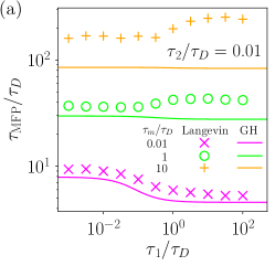
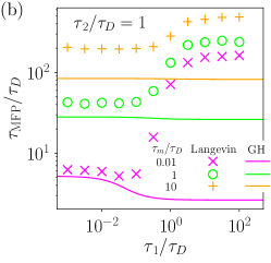
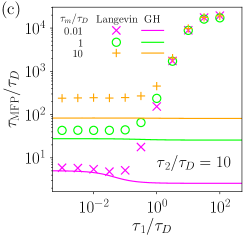
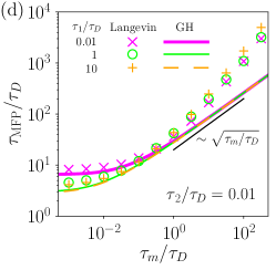
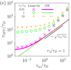
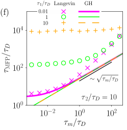
Figure 7: Comparison of numerical MFPTs to Grote-Hynes (GH) theory. (a)-(c) Colored symbols denote the rescaled MFPT $\tau_{\mathrm{MFP}}/\tau_{D}$ as function of $\tau_{1}/\tau_{D}$ for several values of $\tau_{2}/\tau_{D}$ and fixed $\tau_{m}/\tau_{D}$, given by (a) $\tau_{m}/\tau_{D}=0.01$, (b) $\tau_{m}/\tau_{D}=1$, (c) $\tau_{m}/\tau_{D}=10$. The numerical data is the same as shown in Fig. 8. The colored lines represent GH theory, evaluated for a bi-exponential memory kernel using the simulation parameters. (d)-(f) Colored symbols denote the rescaled MFPT $\tau_{\mathrm{MFP}}/\tau_{D}$ as function of $\tau_{m}/\tau_{D}$ for several values of $\tau_{2}/\tau_{D}$ and fixed $\tau_{1}/\tau_{D}$, given by (a) $\tau_{1}/\tau_{D}=0.01$, (b) $\tau_{1}/\tau_{D}=1$, (c) $\tau_{1}/\tau_{D}=10$. The numerical data is a replot of the data shown in Fig. 10. The colored lines represent GH theory, evaluated for a bi-exponential memory kernel using the simulation parameters. The black lines indicate the transition-state-theory (TST) scaling $\tau_{\mathrm{MFP}}/\tau_{D}\sim\sqrt{\tau_{m}/\tau_{D}}$ which GH theory attains in the energy-diffusion regime Grote and Hynes (1980). All data is obtained using $\beta U_{0}=3$.

In Fig. 7 we compare numerical MFPTs to Grote-Hynes (GH) theory Grote and Hynes (1980). Consistent with previous results Kappler et al. (2018), we find that GH theory only describes the numerical MFPTs in the high-friction regime $\tau_{m}/\tau_{D}\ll 1$ and if both memory times are small, $\tau_{1}/\tau_{D},\tau_{2}/\tau_{D}\ll 1$. If either $\tau_{m}/\tau_{D}\gg 1$ or $\min\{\tau_{1}/\tau_{D},\tau_{2}/\tau_{D}\}\gg 1$, then GH theory reduces to the transition state theory (TST) limit where $\tau_{\mathrm{MFP}}/\tau_{D}\sim\sqrt{\tau_{m}/\tau_{D}}$, as can be seen in Figs. 7 (d)-(f). Thus, also for bi-exponential memory GH theory only yields accurate results in the high-friction short-memory regime.

The disagreement between our Langevin results and GH theory is not surprising, since the latter is by construction not intended for the energy diffusion regime. More specifically, GH theory considers a GLE close to the barrier top, so that the theory does not include memory effects from the motion of the particle in the potential well; the GLE model we consider here has a global position-indepedent memory function Pollak et al. (1989). Therefore, only in or close to the overdamped regime, where memory effects from motion in the well are not relevant to the dynamics close to the barrier top, do the predictions of GH theory and our numerical results agree.

Appendix F Global comparison of numerical data to Eq. (7) at $\beta U_{0}=3$

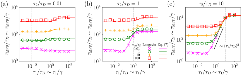
Figure 8: Simulation results for the MFPT at fixed $\tau_{2}/\tau_{D}$. Colored symbols denote the rescaled MFPT $\tau_{\mathrm{MFP}}/\tau_{D}$ as function of $\tau_{1}/\tau_{D}$ for several values of $\tau_{m}/\tau_{D}$ and fixed $\tau_{2}/\tau_{D}$, given by (a) $\tau_{2}/\tau_{D}=0.01$, (b) $\tau_{2}/\tau_{D}=1$, (c) $\tau_{2}/\tau_{D}=10$. The legend for all subplots is given in subplot (b). The colored lines represent the crossover formula Eq. (7), the vertical dashed lines denote where $\tau_{1}=\tau_{2}$. The black bar in (c) indicates the scaling $\tau_{\mathrm{MFP}}\sim\tau_{1}^{2}$ which corresponds to the single-exponential long-memory regime. All data is obtained using $\beta U_{0}=3$.

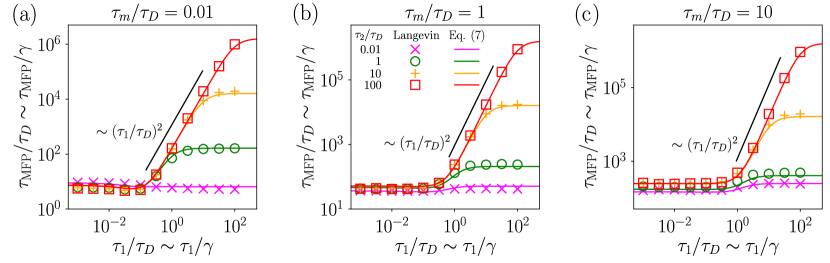
Figure 9: Simulation results for the MFPT at fixed $\tau_{m}/\tau_{D}$. Colored symbols denote the rescaled MFPT $\tau_{\mathrm{MFP}}/\tau_{D}$ as function of $\tau_{1}/\tau_{D}$ for several values of $\tau_{2}/\tau_{D}$ and fixed $\tau_{m}/\tau_{D}$, given by (a) $\tau_{m}/\tau_{D}=0.01$, (b) $\tau_{m}/\tau_{D}=1$, (c) $\tau_{m}/\tau_{D}=10$. The legend for all subplots is given in subplot (b). The colored lines represent the crossover formula Eq. (7), the black bars indicate the scaling $\tau_{\mathrm{MFP}}\sim\tau_{1}^{2}$, which corresponds to the single-exponential long-memory regime. All data is obtained using $\beta U_{0}=3$.

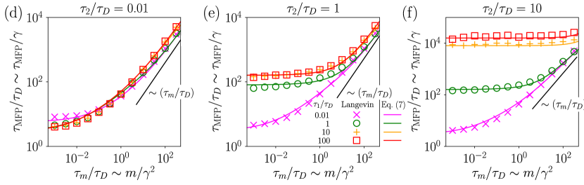
Figure 10: Simulation results for the MFPT at fixed $\tau_{2}/\tau_{D}$. Colored symbols denote the rescaled MFPT $\tau_{\mathrm{MFP}}/\tau_{D}$ as function of $\tau_{m}/\tau_{D}$ for several values of $\tau_{1}/\tau_{D}$ and fixed $\tau_{2}/\tau_{D}$, given by (a) $\tau_{2}/\tau_{D}=0.01$, (b) $\tau_{2}/\tau_{D}=1$, (c) $\tau_{2}/\tau_{D}=10$. The legend for all subplots is given in subplot (b). The colored lines represent the crossover formula Eq. (7), the black bars indicate the scaling $\tau_{\mathrm{MFP}}\sim\tau_{m}$ which corresponds to the Markovian inertial regime. All data is obtained using $\beta U_{0}=3$.

In Figs. 8, 9, 10 we compare predictions of the crossover formula Eq. (7) for $\tau_{\mathrm{MFP}}$ to numerical results. These figures, which we discuss in detail in the following paragraphs, show that Eq. (7) quantitively describes the bi-exponential MFPTs over the whole parameter range of $\tau_{m}/\tau_{D}$, $\tau_{1}/\tau_{D}$, $\tau_{2}/\tau_{D}$ considered, and in particular that the MFPT is in the non-Markovian regime dominated by the shorter memory time.

Figure 8 shows $\tau_{\mathrm{MFP}}/\tau_{D}$ as function of $\tau_{1}/\tau_{D}$ for fixed values of $\tau_{m}/\tau_{D}$, $\tau_{2}/\tau_{D}$. In the figure we see that for $\tau_{1}\ll\tau_{2}$, i.e., to the left of the vertical dashed lines that denote $\tau_{1}=\tau_{2}$, the MFPT behaves similar to the single-exponential MFPT shown in Fig. 4 (b). In particular, for $\tau_{m}/\tau_{D}=0.01$ (magenta crosses) the memory acceleration regime can be seen in Fig. 8 (b), (c) for $\tau_{1}/\tau_{D}\approx 0.1$, followed by the power-law scaling $\tau_{\mathrm{MFP}}/\tau_{D}\sim(\tau_{1}/\tau_{D})^{2}$ for $0.1\lesssim\tau_{1}/\tau_{D}\lesssim\tau_{2}/\tau_{D}$. As $\tau_{1}\gtrsim\tau_{2}$, i.e., to the right of the vertical dashed lines, the MFPT becomes independent of $\tau_{1}$. This can prominently be seen in Fig. 8 (a), where $\tau_{2}/\tau_{D}=0.01$ is small and $\tau_{\mathrm{MFP}}/\tau_{D}$ is almost constant for $\tau_{1}>\tau_{2}$. Throughout Fig. 8 the crossover formula Eq. (7) describes the numerical results very well.

Figure 9 shows $\tau_{\mathrm{MFP}}/\tau_{D}$ as function of $\tau_{1}/\tau_{D}$ for fixed values of $\tau_{2}/\tau_{D}$, $\tau_{m}/\tau_{D}$. In Fig. 9 (a), we again see single-exponential behavior reminiscent of Fig. 4 (b). More explicitly, for $\tau_{2}/\tau_{D}=1$, $10$, $100$, we observe a slight dip in $\tau_{\mathrm{MFP}}/\tau_{D}$ for $\tau_{1}/\tau_{D}\approx 0.1$, followed by power-law scaling $\tau_{\mathrm{MFP}}/\tau_{D}\sim(\tau_{1}/\tau_{D})^{2}$ for $0.1\lesssim\tau_{1}/\tau_{D}\lesssim\tau_{2}/\tau_{D}$. As $\tau_{1}\gtrsim\tau_{2}$, $\tau_{\mathrm{MFP}}/\tau_{D}$ saturates to a value determined by $\tau_{m}/\tau_{D}$, $\tau_{2}/\tau_{D}$. For $\tau_{2}/\tau_{D}=0.01$ (magenta crosses), Fig. 9 (a) contains no regime where $\tau_{1}\ll\tau_{2}$, and $\tau_{\mathrm{MFP}}/\tau_{D}$ is almost independent of $\tau_{1}/\tau_{D}$ throughout. Figs. 9 (b), (c) show similar behavior, and as expected from the single-exponential data for $\tau_{m}/\tau_{D}=1$, $10$ (see Fig. 4 (a)), a dip in the MFPT for $\tau_{1}/\tau_{D}\approx 0.1$ cannot be observed in the logarithmic representation of $\tau_{\mathrm{MFP}}/\tau_{D}$. Again, the crossover formula Eq. (7) describes the data very accurately throughout.

Figure 10 shows $\tau_{\mathrm{MFP}}/\tau_{D}$ as a function of $\tau_{m}/\tau_{D}$ for fixed values of $\tau_{1}/\tau_{D}$, $\tau_{2}/\tau_{D}$. In all three plots, the MFPT displays a similar $\tau_{m}/\tau_{D}$-dependence as the single-exponential case, c.f. Fig. 4 (a). For $\tau_{2}/\tau_{D}=0.01$ we see in Fig. 10 (a) that $\tau_{\mathrm{MFP}}/\tau_{D}$ is almost independent of $\tau_{1}/\tau_{D}$, consistent with the picture that $\tau_{\mathrm{MFP}}/\tau_{D}$ is determined by the shorter memory time $\tau_{2}$. On the other hand, for large $\tau_{2}/\tau_{D}=10$ the MFPT shown in Fig. 10 (c) depends very much on $\tau_{1}/\tau_{D}$ and is qualitatively identical to the single-exponential MFPT shown in Fig. 4 (a). Also for this case, we see that the crossover formula Eq. (7) remains accurate.

Appendix G Comparison of numerical data to Eq. (7) for varying barrier height $\beta U_{0}$

In Fig. 11 we compare predictions of the crossover formula Eq. (7) for $\tau_{\mathrm{MFP}}$ to numerical results, varying the barrier height $\beta U_{0}$. While Fig. 11 (a) considers the symmetric case ($\tau_{\Gamma}\equiv\tau_{1}=\tau_{2}$), Fig. 11 (b) considers the asymmetric scenario ($0.001=\tau_{1}/\tau_{D}\ll\tau_{2}/\tau_{D}=10$). The agreement between Eq. (7) and numerical data in Fig. 11 shows that our heuristic formula accurately describes the Langevin data for barrier heights larger than $\beta U_{0}\approx 2$ throughout.

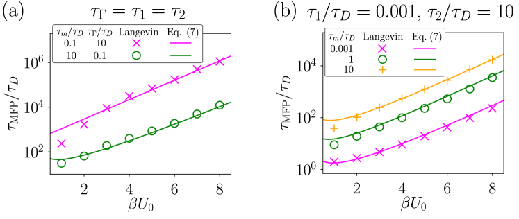
Figure 11: Simulation results for the MFPT as a function of barrier height $\beta U_{0}$. Colored symbols denote the rescaled MFPT $\tau_{\mathrm{MFP}}/\tau_{D}$, obtained from numerical simulations, as function of $\beta U_{0}$ for fixed values of $\tau_{m}/\tau_{D}$, $\tau_{1}/\tau_{D}$, $\tau_{2}/\tau_{D}$; colored solid lines represent the crossover formula Eq. (7). (a) Symmetric scenario $\tau_{\Gamma}\equiv\tau_{1}=\tau_{2}$. (b) Asymmetric scenario with $\tau_{1}/\tau_{D}=0.001$, $\tau_{2}/\tau_{D}=10$. Note that the symmetric scenario has previously been considered in the literature Kappler et al. (2018).

References

- Kramers (1940) H. A. Kramers, Physica 7, 284 (1940).
- Chandler (1986) D. Chandler, Journal of Statistical Physics 42, 49 (1986).
- Berne et al. (1988) B. J. Berne, M. Borkovec, and J. E. Straub, Journal of Physical Chemistry 92, 3711 (1988).
- Hänggi et al. (1990) P. Hänggi, P. Talkner, and M. Borkovec, Reviews of Modern Physics 62, 251 (1990).
- Best and Hummer (2006) R. Best and G. Hummer, Physical Review Letters 96 (2006), 10.1103/PhysRevLett.96.228104.
- Zwanzig (1961) R. Zwanzig, Physical Review 124, 983 (1961).
- Mori (1965) H. Mori, Progress of Theoretical Physics 33, 423 (1965).
- Jung et al. (2017) G. Jung, M. Hanke, and F. Schmid, Journal of Chemical Theory and Computation 13, 2481 (2017), pMID: 28505440, https://doi.org/10.1021/acs.jctc.7b00274 .
- Jung et al. (2018) G. Jung, M. Hanke, and F. Schmid, Soft Matter 14, 9368 (2018).
- Meyer et al. (2017) H. Meyer, T. Voigtmann, and T. Schilling, The Journal of Chemical Physics 147, 214110 (2017), https://doi.org/10.1063/1.5006980 .
- Meyer et al. (2019) H. Meyer, T. Voigtmann, and T. Schilling, The Journal of Chemical Physics 150, 174118 (2019), https://doi.org/10.1063/1.5090450 .
- Rey and Guardia (1992) R. Rey and E. Guardia, The Journal of Physical Chemistry 96, 4712 (1992).
- Mullen et al. (2014) R. G. Mullen, J.-E. Shea, and B. Peters, Journal of Chemical Theory and Computation 10, 659 (2014).
- Rosenberg et al. (1980) R. O. Rosenberg, B. J. Berne, and D. Chandler, Chemical Physics Letters 75, 162 (1980).
- de Sancho et al. (2014) D. de Sancho, A. Sirur, and R. B. Best, Nature Communications 5 (2014), 10.1038/ncomms5307.
- Daldrop et al. (2018a) J. O. Daldrop, J. Kappler, F. N. Brünig, and R. R. Netz, Proceedings of the National Academy of Sciences 115, 5169 (2018a).
- Mason and Weitz (1995) T. G. Mason and D. A. Weitz, Physical Review Letters 74, 1250 (1995).
- Lesnicki et al. (2016) D. Lesnicki, R. Vuilleumier, A. Carof, and B. Rotenberg, Physical Review Letters 116 (2016), 10.1103/PhysRevLett.116.147804.
- Daldrop et al. (2017) J. O. Daldrop, B. G. Kowalik, and R. R. Netz, Physical Review X 7 (2017), 10.1103/PhysRevX.7.041065.
- Berner et al. (2018) J. Berner, B. Müller, J. R. Gomez-Solano, M. Krüger, and C. Bechinger, Nature Communications 9, 999 (2018).
- Selmeczi et al. (2005) D. Selmeczi, S. Mosler, P. H. Hagedorn, N. B. Larsen, and H. Flyvbjerg, Biophysical Journal 89, 912 (2005).
- Wilemski and Fixman (1974) G. Wilemski and M. Fixman, The Journal of Chemical Physics 60, 878 (1974).
- Szabo et al. (1980) A. Szabo, K. Schulten, and Z. Schulten, The Journal of Chemical Physics 72, 4350 (1980).
- Dua and Adhikari (2011) A. Dua and R. Adhikari, Journal of Statistical Mechanics: Theory and Experiment 2011, P04017 (2011).
- Gowdy et al. (2017) J. Gowdy, M. Batchelor, I. Neelov, and E. Paci, The Journal of Physical Chemistry B 121, 9518 (2017).
- Guérin et al. (2012) T. Guérin, O. Bénichou, and R. Voituriez, Nature Chemistry 4, 568 (2012).
- Plotkin and Wolynes (1998) S. S. Plotkin and P. G. Wolynes, Physical Review Letters 80, 5015 (1998).
- Das and Makarov (2018) A. Das and D. E. Makarov, J. Phys. Chem. B 122, 9049 (2018).
- Grote and Hynes (1980) R. F. Grote and J. T. Hynes, The Journal of Chemical Physics 73, 2715 (1980).
- Carmeli and Nitzan (1982) B. Carmeli and A. Nitzan, Physical Review Letters 49, 423 (1982).
- Straub et al. (1986) J. E. Straub, M. Borkovec, and B. J. Berne, The Journal of Chemical Physics 84, 1788 (1986).
- Talkner and Braun (1988) P. Talkner and H.-B. Braun, The Journal of Chemical Physics 88, 7537 (1988).
- Pollak et al. (1989) E. Pollak, H. Grabert, and P. Hänggi, The Journal of Chemical Physics 91, 4073 (1989).
- Ianconescu and Pollak (2015) R. Ianconescu and E. Pollak, The Journal of Chemical Physics 143, 104104 (2015).
- Tucker et al. (1991) S. C. Tucker, M. E. Tuckerman, B. J. Berne, and E. Pollak, The Journal of Chemical Physics 95, 5809 (1991).
- Kappler et al. (2018) J. Kappler, J. O. Daldrop, F. N. Brünig, M. D. Boehle, and R. R. Netz, The Journal of Chemical Physics 148, 014903 (2018).
- Tolokh et al. (2002) I. S. Tolokh, G. W. N. White, S. Goldman, and C. G. Gray, Molecular Physics 100, 2351 (2002).
- Gottwald et al. (2015) F. Gottwald, S. Karsten, S. D. Ivanov, and O. Kühn, The Journal of Chemical Physics 142, 244110 (2015).
- Northrup and Hynes (1980) S. H. Northrup and J. T. Hynes, The Journal of Chemical Physics 73, 2700 (1980).
- Zwanzig (1973) R. Zwanzig, Journal of Statistical Physics 9, 215 (1973).
- Baron et al. (2007) R. Baron, D. Trzesniak, A. H. de Vries, A. Elsener, S. J. Marrink, and W. F. van Gunsteren, ChemPhysChem 8, 452 (2007).
- Potoyan et al. (2013) D. A. Potoyan, A. Savelyev, and G. A. Papoian, WIREs Comput Mol Sci 3, 69 (2013).
- Marx et al. (1999) D. Marx, M. E. Tuckerman, J. Hutter, and M. Parrinello, Nature 397, 601 (1999).
- Daldrop et al. (2018b) J. O. Daldrop, M. Saita, M. Heyden, V. A. Lorenz-Fonfria, J. Heberle, and R. R. Netz, Nature Communications 9 (2018b), 10.1038/s41467-017-02669-9.
- Chung and Eaton (2013) H. S. Chung and W. A. Eaton, Nature 502, 685 (2013).
- Laleman et al. (2017) M. Laleman, E. Carlon, and H. Orland, J. Chem. Phys. 147, 214103 (2017).
- Mel’nikov and Meshkov (1986) V. I. Mel’nikov and S. V. Meshkov, The Journal of Chemical Physics 85, 1018 (1986).
- Hänggi and Weiss (1984) P. Hänggi and U. Weiss, Phys. Rev. A 29, 2265 (1984).
- Carmeli and Nitzan (1984) B. Carmeli and A. Nitzan, Phys. Rev. A 29, 1481 (1984).
- Straub et al. (1985) J. E. Straub, M. Borkovec, and B. J. Berne, The Journal of Chemical Physics 83, 3172 (1985), https://doi.org/10.1063/1.449172 .
- Grabert et al. (1988) H. Grabert, P. Schramm, and G.-L. Ingold, Physics Reports 168, 115 (1988).
- Kappler et al. (2019) J. Kappler, F. Noé, and R. R. Netz, Phys. Rev. Lett. 122, 067801 (2019).
- Marx (2006) D. Marx, ChemPhysChem 7, 1848 (2006).
- Reimann et al. (1999) P. Reimann, G. J. Schmid, and P. Hänggi, Physical Review E 60, R1 (1999).