Response and Sensitivity Using Markov Chains

Abstract

Dynamical systems are often subject to forcing or changes in their governing parameters and it is of interest to study how this affects their statistical properties. A prominent real-life example of this class of problems is the investigation of climate response to perturbations. In this respect, it is crucial to determine what the linear response of a system is as a quantification of sensitivity. Alongside previous work, here we use the transfer operator formalism to study the response and sensitivity of a dynamical system undergoing perturbations. By projecting the transfer operator onto a suitable finite dimensional vector space, one is able to obtain matrix representations which determine finite Markov processes. Further, using perturbation theory for Markov matrices, it is possible to determine the linear and nonlinear response of the system given a prescribed forcing. Here, we suggest a methodology which puts the scope on the evolution law of densities (the Liouville/Fokker-Planck equation), allowing to effectively calculate the sensitivity and response of two representative dynamical systems.

I Introduction

Response theory is the scientific research area at the boundary between mathematics and physics dealing with the understanding of how complex systems react to perturbations affecting their dynamics. Even if it addresses is a very classical problem, the mathematical framework to develop such a theory is still a matter of research.

Although the construction of response theory can be approached by taking many different scientific point of views, it has been mostly driven by statistical mechanicsMarconi et al. (2008). In this context, by considering a complex system in a steady state (equilibrium or nonequilibrium) and applying some sort of forcing to the dynamics as, e.g., a change in the governing parameters, one is interested in analysing the resulting deviation from the steady state and, in some cases, its relaxation to the new one.

We can express these ideas formally as follows. Let $\{\phi^{t}\}_{t\geq 0}$ be a dynamical system on a compact domain $X\subset\mathbb{R}^{d}$ generated by the evolution equation $\dot{\mathbf{x}}=\mathbf{F}(\mathbf{x})$. We take here the continuous time point of view but one can equivalently formulate the problem for discrete dynamics. Furthermore, let $\mathcal{J}:X\longrightarrow\mathbb{R}$ denote a generic observable. Assuming that the system is in a steady state, we want to analyse the how the values of the observable $\mathcal{J}$ change when the dynamics are subject to a perturbation of the form:

$$\dot{\mathbf{x}}=\mathbf{F}(\mathbf{x})+\epsilon\mathbf{G}(\mathbf{x}),$$ (1)

where $\epsilon\in\mathbb{R}$ is the perturbation parameter and $\mathbf{G}$ is the perturbation vector-field, which is assumed to generate (together with $\mathbf{F}$) the perturbed dynamical system $\{\phi^{t}_{\epsilon}\}_{t\geq 0}$. Thus, the value of the observable $\mathcal{J}$ will change as a result of the perturbation in the following fashion:

$$\frac{d}{dt}\mathcal{J}(\mathbf{x})=\mathbf{F}(\mathbf{x})\cdot\nabla\mathcal{J}(\mathbf{x})+\epsilon\mathbf{G}(\mathbf{x})\cdot\nabla\mathcal{J}(\mathbf{x}).$$ (2)

This equation describes how the observable changes with time, but only upon integration of the perturbed system can we know what its expected value is. The question we, thus, want to address is that of understanding and predicting the mean behaviour of quantities of interest upon modification of the governing dynamics.

In a complex system evolving with time, the mathematical object that accounts for the statistical description of its asymptotic regime is the invariant measureLasota and Mackey (1994). This measure is called invariant because it does not change under the action of the system. Roughly speaking, it tells us how mass is distributed on phase-space in the far future. Thus, if a system is undergoing perturbations, its invariant measure will change and consequently, the expected value of the observables of interest. If the perturbation parameter $\epsilon$ is small enough, one can ask about the effect of the perturbation on the system at a given order of nonlinearity, this is, the response.

Let $\rho$ and $\rho_{\epsilon}$ denote the unperturbed and perturbed measures respectively. If we use the notation introduced earlier, we would like to compute the expectation value of the observable $\mathcal{J}$ in the perturbed steady state $\left\langle\rho_{\epsilon},\mathcal{J}\right\rangle$ in terms of its former expectation value $\left\langle\rho,\mathcal{J}\right\rangle$ and suitable linear and nonlinear correction terms:

$$\left\langle\rho_{\epsilon},\mathcal{J}\right\rangle=\left\langle\rho,\mathcal{J}\right\rangle+\sum_{k=1}^{\infty}\epsilon^{k}\delta[\mathcal{J}]_{k}.$$ (3)

If one has access to $\delta[\mathcal{J}]_{k}$, one could effectively predict what the expected value in the perturbed system and describe its sensitivity to a certain perturbation.

In an isolated system in equilibrium governed by a Hamiltonian, R. KuboKubo (1957) found a closed set of formulas for the response describing $\delta[\mathcal{J}]_{k}$ and establishing the connection with the fluctuation-dissipation theorem (FDT). Such theorem can be seen as a dictionary allowing for predicting the response of a system from its free fluctuations. However, the nature of the problem tackled in Kubo’s work did not allow to extend it to a more general case of nonequilibrium complex systems and the validity of the formulas was not fully addressed. In fact, deterministic dynamical systems featuring contraction of the phase-space posses invariant measures that are singular with respect to the Lebesgue measure. The absence of a regular density is a major barrier that makes impossible the straightforward application of the FDT, thus breaking the one-to-one connection between forced and free fluctuations of a system.

In the work by D. RuelleRuelle (1997, 2009), such framework was clarified at a mathematical level, allowing to apply response theory in nonequilibrium systems. Ruelle’s results are based on the use of Markov partitions and provide a rigorous response theory for Axiom AEckmann and Ruelle (1985) systems. Essential ingredients for the theory are the fact that the unperturbed system are structurally stable and that one can split the response operator in two parts. One refers to the contribution coming from the unstable and central manifolds and can be framed as an FDT result. The second contribution comes from the stable manifold and gives an additional term that cannot be described using the free fluctuations of the system. Hence, a suitable notion of differentiability of singular measures was established allowing to consider perturbative expansions as in Eq. (3) for a general class of deterministic dynamical systems.

The Ruelle response theory has provided a key framework for constructing algorithms aimed at practically computing the response of nonequilibrium systems to perturbations, see e.g. Ref. Abramov and Majda, 2007, and, specifically, for performing successfully climate change predictions using simple, see e.g. Ref. Gritsun and Lucarini, 2017, and comprehensive climate models, see e.g. Refs. Ragone, Lucarini, and Lunkeit, 2016; Lucarini, Lunkeit, and Ragone, 2017.

Despite a good degree of success in the above mentioned studies, the presence of the two distinct contributions described above makes the construction of accurate response algorithms very challenging, see discussion in Ref. Gritsun and Lucarini, 2017. A different point of view, based on the study of the evolution of probabilities rather than of individual trajectories, seems necessary; see below.

I.1 The Transfer Operator Approach

Indeed, one can understand response theory by means of studying the effect of perturbations on the evolution of measures on phase-space as opposed to trajectories. Formulating response theory under this point of view uses essentially different machinery mostly hovering around the so called transfer operatorBaladi (2000).

Let us suppose that $\mathbf{F}:X\subseteq\mathbb{R}^{d}\longrightarrow\mathbb{R}^{d}$ is a vector-field that generates the dynamical system or flow $\{\phi^{t}\}_{t\in\mathbb{R}}$, with $\phi^{t}:X\longrightarrow X$. Then, the transfer operator semigroup $\{\mathcal{L}^{t}\}_{t\geq 0}$ can be defined as the solution of the Liouville equationLasota and Mackey (1994):

$$\partial_{t}\rho(\mathbf{x},t)=-\nabla\cdot\left(\mathbf{F}\rho(\mathbf{x},t)\right),$$ (4)

so that $\rho(\mathbf{x},t)=\mathcal{L}^{t}\rho_{0}(\mathbf{x})$ for some initial condition $\rho_{0}\in L^{1}(X)$. In the language of probability, the transfer operator is describing the pushforward of an integrable function under the action of the dynamical system after $t$ time-units. It turns out that $\mathcal{L}^{t}$ is a contraction and the set $\{\mathcal{L}^{t}\}_{t\geq 0}$ is a $C_{0}$-semigroup Engel and Nagel (2006).

Eq. (4) symbolises a process where mass is only advected along the flow. However, in many areas and applications, the governing dynamics are stochasticly perturbed introducing uncertainty to the problem. This sort of perturbations can be modelled by stochastic processes of the form:

$$\dot{\mathbf{x}}=\mathbf{F}(\mathbf{x})+\Sigma(\mathbf{x})dW_{t},$$ (5)

where we introduce here a standard $d$-dimensional Wiener process $dW_{t}$ and $\Sigma(\mathbf{x})\in\mathbb{R}^{d\times d}$ is the covariance matrix. In terms of measures, stochasticity can be translated into the fact that their evolution is not only driven by advection, but diffusion is present. The Liouville is thus transformed into the Fokker-Planck equationRisken (1989):

$$\partial_{t}\rho(\mathbf{x},t)=\mathcal{A}\rho(\mathbf{x},t):=-\nabla\cdot\left(\mathbf{F}\rho(\mathbf{x},t)\right)+\frac{1}{2}\sum_{i=1}^{d}\sum_{j=1}^{d}\partial_{x_{i},x_{j}}\Sigma\Sigma^{\ast}(\mathbf{x})\rho(\mathbf{x},t).$$ (6)

We have defined the differential operator $\mathcal{A}$ which can be shown to generate a $C_{0}$-semigroup, just as the Liouville equation does. Notice that the differential operator on the right-hand-side of Eq. (4) is the same as $\mathcal{A}$ if no noise is present.

The transfer operator is therefore a statistical tool rather than a dynamical one. It globally describes how densities evolve with time as opposed of giving a trajectory-wise description of the system. In fact, the spectral properties of the transfer operator carry information about the statistical properties of the system of interest. For instance, one observes that the fixed points of $\mathcal{L}^{t}$ are nothing else than the measure that remain fixed under the action of the dynamics, namely, the invariant measure. In fact, the ergodicity and mixing character of a dynamical system can be characterised in terms of the nature of the leading eigenvalues of $\mathcal{L}^{t}$ (e.g. Ref. Baladi, 2000).

Introducing perturbations on the system not only does it affect to the way trajectories evolve on phase-space but also to measures. This is reflected on the Fokker-Planck evolution equation where by considering a perturbation on the vector-field of the kind $\mathbf{F}\mapsto\mathbf{F}+\sum_{k}\epsilon_{k}\mathbf{G}_{k}$ we obtain a perturbed evolution law for the density:

$$\partial_{t}\rho(\mathbf{x},t)=\mathcal{A}\rho(\mathbf{x},t)+\sum_{k=1}^{n}\epsilon_{k}\mathcal{B}_{k}\rho(\mathbf{x},t),$$ (7)

where $\mathcal{B}_{k}=-\nabla\cdot\left(\mathbf{G}_{k}\circ\right)$. Under some conditionsEngel and Nagel (2006) the previous equation also generates a $C_{0}$-semigroup with the same functional properties as the unperturbed one. One can also introduce perturbations on the covariance matrix, which would lead to a similar equation as the one above with different perturbation operators.

Projected Transfer Operators and Markov Chains

The transfer operator has been used to solve problems in different areas of science, see e.g. examples in geosciences Refs. Tantet et al., 2018; Tantet, van der Burgt, and Dijkstra, 2015; Froyland et al., 2007. In these applications phase-space is not defined as a continuum but as finite collection of regions. As a result, each time the transfer operator is applied, a finite probability mass is shifted from one region to another one. For this reason, in applications, the transfer operator has to be understood in a finite dimensional setting.

To do this, we shall consider a finite subdivision of phase-space $X$ into $N$ regions or boxes $\{B_{i}\}_{i=1}^{N}$ and define $\mathbf{1}_{B_{i}}$ as the characteristic function on box $B_{i}\subset X$. Thus, we define the projection $P_{N}:L^{1}\left(X\right)\longrightarrow U_{N}:=\mathrm{Span}\left(\{\mathbf{1}_{B_{i}}\}_{i=1}^{N}\right)$ as

$$P_{N}\rho=\sum_{i=1}^{N}\frac{\mathbf{1}_{B_{i}}}{\eta\left(B_{i}\right)}\int_{B_{i}}\rho\mathbf{1}_{B_{i}}\eta(dx),$$ (8)

where $\eta$ indicates some notion of volume that can depend on the problem. It follows that the operator $P_{N}\mathcal{L}^{t}:U_{N}\longrightarrow U_{N}$ admits a matrix representation:

$$\mathcal{M}^{t}_{i,j}:=\left(P_{N}\mathcal{L}^{t}\right)_{i,j}=\frac{1}{\eta(B_{i})}\int_{B_{i}}\mathcal{L}^{t}\mathbf{1}_{B_{j}}\eta(dx),$$ (9)

which happens to be a Markov or stochastic matrix. The way we practically construct $\mathcal{M}^{t}$ depends on the choice of measure $\eta$. Generally, if one wants to study the asymptotic properties of the system one will take $\eta$ as the invariant measure. On the other hand, if the focus is put on the effects of the flow on the whole domain $X$, and especially if one is interested in problems of relaxation to the steady state, the correct choice would be to consider the Lebesgue measure insteadTantet, Lucarini, and Dijkstra (2018). It is worth highlighting that the properties of the dynamical system $\phi^{t}$ are described by $\mathcal{L}^{t}$.

Perturbations on the dynamics lead to perturbations on the transfer operator $\mathcal{L}^{t}$ and, consequently on the matrix $\mathcal{M}^{t}$. This fact motivates the problem of reverting the question, i.e., by considering perturbations of $\mathcal{M}^{t}$, what can we say about the dynamics? This question has been tackled in previous work Lucarini (2016); Froyland, Antown, and Cevi (2018) by suitably constructing the response operators. Alongside the development of the probabilistic theory, it was possible to establish a connection between the perturbation theory of Markov chains and linear response theory for dynamical systems, applying it to a number of low dimensional stochastic and deterministic dynamical systems.

Constructing the operator that accounts for the linear response can be a difficult and costly taskAbramov and Majda (2007). Linear response can be inferred by examining how the system of interest responds to small perturbations in the governing equations. However, this process can be an expensive procedure if one deals with high-dimensioinal models with physical relevance. Therefore, one desires to have predictive power. In this paper we demonstrate that it is possible to calculate, by using finite representations of the transfer operator, the response of a system by sampling its unperturbed dynamics and prior knowledge of the forcings applied to it. The overall goal is to provide practically usable tools for studying the response of complex nonequilibrium system, like the climate, to perturbations. In Section II we will present the perturbation theory for Markovian matrices, key to construct the response operator at a coarse-grained level. In Section III we investigate how to put into practise such theory when dealing with continuous in time dynamical systems and illustrate the applicability of the methodology with two dynamical systems of interest.

II Perturbations of Finite Markov Chains

In this section, we consider a mixing (therefore, ergodic) Markov process with a finite number of states $N\in\mathbb{N}$. Then, a positive vector $\mathbf{u}_{0}\in\mathbb{R}^{N}$ with $\sum_{i=1}^{N}\left(\mathbf{u}_{0}\right)_{i}=1$ would indicate an initial ensemble of states. The finite Markov process would be determined by a stochastic matrix $\mathcal{M}\in\mathbb{R}^{N\times N}$ so that the sequence $\{\mathcal{M}^{n}\mathbf{u}_{0}\}_{n=0}^{\infty}$ would be a realisation of it.

The stochastic matrix $\mathcal{M}$ enjoys some properties worth highlighting. First, we note that $\mathcal{M}_{i,j}$ is the probability of jumping into the $i$th state conditioned on being at the $j$th. Thus, it follows that

$$\sum_{i=1}^{N}\mathcal{M}_{i,j}=1,$$ (10)

for any $j=1,\ldots,N$. Therefore, all the entries of $\mathcal{M}$ are greater than or equal to zero. Further, since the process is mixing, it implies that there exists $p\in\mathbb{N}$, so that the entries of the matrix $\mathcal{M}^{p}$ are strictly greater than zero Seneta (1973). Matrices satisfying this condition are called irreducible and aperiodicBaladi (2000) or primitiveSeneta (1973), although we shall refer to them as mixing by analogy with the Markov process they determine. Consequently, the Perron-Frobenius theoremSeneta (1973) holds for this matrix, meaning that there exists a leading eigenvalue $\lambda_{1}$ with positive eigenvector $\mathbf{u}$. By virtue of the spectral properties of stochastic matrices, it turns out that $\lambda_{1}=1$ and $\mathbf{u}$ solves

$$\mathcal{M}\mathbf{u}=\mathbf{u}.$$ (11)

This means that $\mathbf{u}$ remains invariant under the action of $\mathcal{M}$. If, in addition, $\mathbf{u}$ is normalised so that its entries sum up to one, we call $\mathbf{u}$ the invariant measure of the process and it follows that $\lim_{p\rightarrow\infty}\mathcal{M}^{p}\mathbf{u}_{0}=\mathbf{u}$, for any normalised non-zero vector $\mathbf{u}_{0}\in\mathbb{R}^{N}$.

The next step now is to perturb the stochastic matrix and express the resulting perturbed invariant measure as a perturbative expansion. In what follows, we generalise what reported in Ref. Lucarini, 2016. For that, we consider a perturbation of $\mathcal{M}$ of the form:

$$\mathcal{M}\longrightarrow\mathcal{M}+\sum_{i=1}^{n}\epsilon_{k}m_{k},$$ (12)

where $\epsilon_{1},\ldots,\epsilon_{n}\in\mathbb{R}$ and $m_{1},\ldots,m_{n}\in\mathbb{R}^{N\times N}$. The matrices $m_{k}$ are what we will call the perturbation matrices. Note that the perturbed matrix $\mathcal{M}+\sum_{k=1}^{n}\epsilon_{k}m_{k}$, must also be a stochastic matrix if we want it to describe a Markov process. This requirement corresponds to having

$$\sum_{i=1}^{N}\left(m_{k}\right)_{i,j}=0,$$ (13)

for any $k$ and $j$. This assures that the columns of $\mathcal{M}+\sum_{k=1}^{n}\epsilon_{k}m_{k}$ add up to one. More, non-negativity must be preserved, so not all choices of $\epsilon_{k}$ are valid. For this, we define

$$\epsilon^{-}=\min\{\epsilon\in\mathbb{R}:\forall i,j\in\{1,\ldots,N\},\mathcal{M}_{i,j}+\epsilon\sum_{k=1}^{n}\left(m_{k}\right)_{i,j}\geq 0\},$$ (14)

and

$$\epsilon^{+}=\max\{\epsilon\in\mathbb{R}:\forall i,j\in\{1,\ldots,N\},\mathcal{M}_{i,j}+\epsilon\sum_{k=1}^{n}\left(m_{k}\right)_{i,j}\geq 0\}.$$ (15)

Hence, to ensure non-negativity of the perturbed Markov process, we must have that $\max_{k}\epsilon_{k}\in\left[\epsilon^{-},\epsilon^{+}\right]$. To ensure that the latter interval is non-empty, we need to make sure that $\epsilon^{-}<0$ and $\epsilon^{+}>0$. Suppose that $\mathcal{M}_{i_{1},j_{1}}=\mathcal{M}_{i_{2},j_{2}}=0$ and $\left(\sum_{k}m_{k}\right)_{i_{1},j_{1}},\left(\sum_{k}m_{k}\right)_{i_{2},j_{2}}<0$. This would imply that $\epsilon^{-}=\epsilon^{+}=0.$ In this case, we have non-admissible perturbations.

Again, by virtue of the Perron-Frobenius theorem, such perturbed matrix will have a dominant eigenvalue, whose value is $1$ and its associated eigenvector $\mathbf{v}=\mathbf{v}(\epsilon_{1},\ldots,\epsilon_{n})$ is strictly positive. In other words, $\mathbf{v}$ solves:

$$\left(\mathcal{M}+\sum_{k=1}^{n}\epsilon_{k}m_{k}\right)\mathbf{v}=\mathbf{v}.$$ (16)

The goal is to express the perturbed invariant measure $\mathbf{v}$ in terms of $\mathcal{M},m_{1},\ldots,m_{n},\epsilon_{1},\ldots$ and $\epsilon_{n}$. Not only do we want to calculate $\mathbf{v}$ but also describe how the unperturbed measure $\mathbf{u}$ responds at a given power of $\epsilon_{k}$.

Using multiindex notation, we suppose a formal expansion in powers of $\epsilon_{1},\ldots,\epsilon_{n}$:

$$\mathbf{v}=\mathbf{u}+\sum_{|\alpha|=1}^{\infty}(\epsilon_{1},\ldots,\epsilon_{n})^{\alpha}\mathbf{w}_{\alpha},$$ (17)

where $\mathbf{w}_{\alpha}=\frac{1}{\alpha!}\left(\partial_{\epsilon_{1}},\ldots,\partial_{\epsilon_{n}}\right)^{\alpha}$. Substituting this expression in Eq. (16) we obtain:

$$\left(\mathcal{M}+\sum_{k=1}^{n}\epsilon_{k}m_{k}\right)\left(\mathbf{u}+\sum_{|\alpha|=1}^{\infty}(\epsilon_{1},\ldots,\epsilon_{n})^{\alpha}\mathbf{w}_{\alpha}\right)=\mathbf{u}+\sum_{|\alpha|=1}^{\infty}(\epsilon_{1},\ldots,\epsilon_{n})^{\alpha}\mathbf{w}_{\alpha}.$$ (18)

Gathering the terms for $|\alpha|=1$ we get:

$$\mathcal{O}(\epsilon_{k}):\left(1-\mathcal{M}\right)\partial_{\epsilon_{k}}\mathbf{v}=m_{k}\mathbf{u},$$

for $k=1,\ldots,n$. The matrix $1-\mathcal{M}$ cannot be inverted since $1$ is an eigenvalue of $\mathcal{M}$; we shall discuss this issue in the next section. At the moment, we directly apply the inverted matrix to find that

$$\partial_{\epsilon_{k}}\mathbf{v}=\left(1-\mathcal{M}\right)^{-1}m_{k}\mathbf{u}.$$ (19)

We define $\Psi_{k}=\left(1-\mathcal{M}\right)^{-1}m_{k}$ as linear response operator. This matrix has also been named a differential matrixSchweitzer (1968). If we repeat the process for the second order terms ($|\alpha|=2$) we get:

$$\mathcal{O}\left(\epsilon_{k}^{2}\right):\frac{1}{2!}\partial^{2}_{\epsilon_{k}}\mathbf{v} =\left(1-\mathcal{M}\right)^{-1}m_{k}\partial_{\epsilon_{k}}\mathbf{v}=\left(\Psi_{k}\right)^{2}\mathbf{u}$$

$$\mathcal{O}\left(\epsilon_{k}\epsilon_{l}\right):\partial^{2}_{\epsilon_{k},\epsilon_{l}}\mathbf{v} =\left(1-\mathcal{M}\right)^{-1}m_{l}\partial_{\epsilon_{k}}\mathbf{v}+\left(1-\mathcal{M}\right)^{-1}m_{k}\partial_{\epsilon_{l}}\mathbf{v}$$

$$=\Psi_{k}\Psi_{l}\mathbf{u}+\Psi_{l}\Psi_{k}\mathbf{u}.$$

Thus, we inductively construct the whole expansion as:

$$\mathbf{v} =\mathbf{u}+\sum_{i=1}^{\infty}\left(\sum_{k=1}^{n}\epsilon_{k}\Psi_{k}\right)^{i}\mathbf{u}=\left(1-\sum_{k=1}^{n}\epsilon_{k}\Psi_{k}\right)^{-1}\mathbf{u}.$$ (20)

This formula provides a tool to predict the perturbed invariant measure for as long as it converges. Perturbative formulas like this were found in the probability literatureSchweitzer (1968) and later revisited when linking them to the study of the response of dynamical systemsLucarini (2016); Froyland, Antown, and Cevi (2018).

Moreover, by simply considering the adjoint matrices, it is possible to develop a response theory for observables. Indeed, let $\mathcal{J}\in\mathbb{R}^{N}$ represent a generic coarse-grained observable. Then, its expectation value with respect to the perturbed stationary vector $\mathbf{v}$ satisfies:

$$\left\langle\mathcal{J},\mathbf{v}\right\rangle=\left\langle\mathcal{J},\mathbf{u}+\sum_{i=1}^{\infty}\left(\sum_{k=1}^{n}\epsilon_{k}\Psi_{k}\right)^{i}\mathbf{u}\right\rangle=\left\langle\left(1+\sum_{i=1}^{\infty}\left(\sum_{k=1}^{n}\epsilon_{k}\Psi_{k}\right)^{i}\right)^{\top}\mathcal{J},\mathbf{u}\right\rangle=\left\langle 1+\sum_{i=1}^{\infty}\left(\sum_{k=1}^{n}\epsilon_{k}\Psi_{k}^{\top}\right)^{i}\mathcal{J},\mathbf{u}\right\rangle,$$ (21)

where $\left\langle\cdot,\cdot\right\rangle$ denotes the pairing between measures and observables. The advantage of formulas (20) and (21) is that they allow us to identify the response to perturbations at an arbitrary order of nonlinearity including the linear case, which has a special relevance in the physical literature. As a consequence, if one is interested in calculating the sensitivity of the expectation value of some observable $\mathcal{J}$ with respect to changes caused by $\epsilon_{k}m_{k}$, one has to truncate the series expansion in the first order term. However, these formulas are still purely formal. We need a deeper understanding of what we mean with $\left(1-\mathcal{M}\right)^{-1}$ and for what values of $\epsilon_{k}$ they are useful.

II.1 Well-posedness and Invertibility of $1-\mathcal{M}$

In this section we will clarify the framework for which the response formulas presented above work. First of all, we will revisit the problem of the non-invertibility of $1-\mathcal{M}$. Secondly, we will assess the convergence of the power expansion in Eq. (20) and include a comment on the stability of the leading eigenvalues of $\mathcal{M}$.

The linear response operator is not well defined a priori as $1$ is an eigenvalue of the matrix $\mathcal{M}$ and hence $1-\mathcal{M}$ is not invertible. However, we can define a more suitable normed space for which the norm of $\mathcal{M}$ is less than one, making $1-\mathcal{M}$ invertible. The idea relies on the fact that the vector space $\mathbb{R}^{N}$ on which $\mathcal{M}$ is defined admits a splitting of the form:

$$\mathbb{R}^{N}=\mathrm{Span}\left(\mathbf{u}\right)\oplus V,$$ (22)

where $V$ is the invariant subspace generated by the generalised eigenvectors of $\mathcal{M}$ associated with the eigenvalues distinct to $1$ and $\mathrm{Span}\left(\mathbf{u}\right)$ is the vector subspace spanned by $\mathbf{u}$. This space can also be regarded as the kernel of the functional $\iota:\mathbb{R}^{N}\longrightarrow\mathbb{R}$ given by $\iota\left(\mathbf{x}\right)=\sum_{i}(\mathbf{x})_{i}$. Indeed, one observes that if $\mathbf{u}_{k}$ is a generalised eigenvector of $\mathcal{M}$, the identity $\left(\mathcal{M}-\lambda_{k}\right)^{p}\mathbf{u}_{k}=\mathbf{0}$ holds for some $p\in\mathbb{N}$. Hence,

$$\iota\left(\left(\mathcal{M}-\lambda_{k}\right)^{p}\mathbf{u}_{k}\right) =\sum_{j=0}^{p}\begin{pmatrix}p\\ j\end{pmatrix}\lambda^{j}_{k}\iota\left(\mathcal{M}^{p-j}\mathbf{u}_{k}\right)$$

$$=\left(1-\lambda^{p}_{k}\right)\iota(\mathbf{u}_{k})=0.$$

This implies that $\iota(\mathbf{u}_{k})=0$, by virtue of the mixing hypothesis. Furhtermore, noting that $\iota\left(m_{k}\mathbf{x}\right)=0$ for any $\mathbf{x}\in\mathbb{R}^{N}$, we can summarise the idea in the following statement:

Proposition II.1

Let $\mathcal{M}\in\mathbb{R}^{N\times N}$ be a mixing stochastic matrix with invariant measure $\mathbf{u}$. Then, for any $\mathbf{x}\in\mathbb{R}^{N}$, $m_{k}\mathbf{x}\in V$ and $1-\mathcal{M}$ is invertible on $V$.

Recall that the linear response operator in Eq. (19) only requires the evaluation of $\left(1-\mathcal{M}\right)^{-1}$ after having calculated $m_{k}\mathbf{u}$, so writing the inverse explicitly is not that big an abuse. However, we must underline that, numerically, we cannot directly invert $1-\mathcal{M}$. To overcome this problem, we must deflate the matrix, removing the dependence on the dominant eigenspace. Concretely, we have to consider the group inverseFunderlic and Meyer (1986) $\mathcal{Z}$ of a Markov chain, which is defined as follows:

$$\mathcal{Z}=\left(1-\mathcal{M}+\mathcal{M}^{\infty}\right)^{-1},$$ (23)

where the matrix $\mathcal{M}^{\infty}$ is defined as $\lim_{p\rightarrow\infty}\mathcal{M}^{p}$. This matrix can be shown to be equal to the matrix whose columns are all equal to the invariant measure $\mathbf{u}$. Intuitively, $\mathcal{M}^{\infty}$ can be seen as a rank-one projector onto $\mathrm{span}\left(\mathbf{u}\right)$. In fact, $1$ is not an eigenvalue of $\mathcal{M}-\mathcal{M}^{\infty}$, making $1-\mathcal{M}+\mathcal{M}^{\infty}$ invertible. The linear response operator is, thus, given by

$$\partial_{\epsilon_{k}}\mathbf{v}=\Psi_{k}\mathbf{u}=\left(1-\mathcal{M}\right)^{-1}m_{k}\mathbf{u}=\mathcal{Z}m_{k}\mathbf{u}.$$ (24)

This way we find a practical way of computing the linear response operator.

To assess convergence, we want to be certain that the $L^{1}$ norm of the series $\sum_{k=1}^{\infty}\left(\epsilon_{1}\Psi_{1}+\ldots+\epsilon_{n}\Psi_{n}\right)^{k}$ does not go to infinity. For this problem we introduce the matrix norm $\|\cdot\|_{1^{\ast}}$ which we define as the norm $\|\cdot\|_{1}$ restricted to $V$. We are now in conditions of applying the ratio test in Eq. (20):

$$\frac{\left\|\left(\sum_{k}\epsilon_{k}\Psi_{k}\right)^{i+1}\mathbf{u}\right\|_{1}}{\left\|\left(\sum_{k}\epsilon_{k}\Psi_{k}\right)^{i}\mathbf{u}\right\|_{1}} =\frac{\left\|\left(\sum_{k}\epsilon_{k}\Psi_{k}\right)\left(\sum_{k}\epsilon_{k}\Psi_{k}\right)^{i}\mathbf{u}\right\|_{1}}{\left\|\left(\sum_{k}\epsilon_{k}\Psi_{k}\right)^{i}\mathbf{u}\right\|_{1}}\leq\left\|\sum_{k=1}^{n}\epsilon_{k}\Psi_{k}\right\|_{1}=\left\|\left(1-\mathcal{M}\right)^{-1}\sum_{k=1}^{n}\epsilon_{k}m_{k}\right\|_{1}\leq\left\|\left(1-\mathcal{M}\right)^{-1}\right\|_{1^{\ast}}\left\|\sum_{k=1}^{n}\epsilon_{k}m_{k}\right\|_{1}$$

$$\leq\left(1-\|\mathcal{M}\|_{1^{\ast}}\right)^{-1}\left\|\sum_{k=1}^{n}\epsilon_{k}m_{k}\right\|_{1}\leq\left(1-\|\mathcal{M}\|_{1^{\ast}}\right)^{-1}\max_{k}\{\epsilon_{k}\}n\max_{k}\{\|m_{k}\|_{1}\}.$$

Since we want that the ratio remains lower than $1$ to ensure (absolute) convergence, we choose $\epsilon_{1},\ldots,\epsilon_{n}$ so that

$$|\max_{k}\{\epsilon_{k}\}|<\epsilon_{max}:=\frac{1-\|\mathcal{M}\|_{1^{\ast}}}{n\max_{k}\{\|m_{k}\|_{1}\}}.$$ (25)

By referring to the mixing character of $\mathcal{M}$ we conclude that $\epsilon_{max}$ is finite and positive. Hence, $\epsilon_{max}$ establishes a tolerance on the size of the perturbation. We would like to underline that the condition for these response formulas to work can be translated to the fact that one requires that the system has to mix mass sufficiently quickly.

The number $\left\|\mathcal{M}\right\|_{1^{\ast}}$ is known as the ergodicity coefficientSeneta (1979) and can serve as a condition number for the Markov chain in the sense that this quantity serves to estimate the norm of the difference between a perturbed and the unperturbed invariant measuresSeneta (1993). See Ref. Inubushi, 2019 for a practical use of the ergodicity coefficient. However, the ergodicity coefficient does not tell us how perturbations affect the localisation of the eigenvalues of the matrix $\mathcal{M}$, something crucial if one wants to control the spectral gap. This problem is tackled by means of analysing the stability of the leading non-unit eigenvalues and summarised in the following result found in Ref. Mitrophanov, 2003:

Proposition II.2

Let $\mathcal{M}\in\mathbb{R}^{N\times N}$ be a diagonalisable, irreducible and aperiodic stochastic matrix. Let $X\in\mathbb{R}^{N\times N}$ be a non-singular matrix such that $\mathcal{M}=X^{-1}\Lambda X$ with $\Lambda$ being the diagonal matrix containing the eigenvalues $1,\lambda_{2},\ldots,\ldots\lambda_{N}$, of $\mathcal{M}$. Suppose that

$$\kappa(X)\max_{k}\{|\epsilon_{k}|\}n\max_{k}\{\|m_{k}\|\}<\frac{1}{2}\min_{1\leq j\leq N}\{1-|\lambda_{j}|\}.$$ (26)

Then, the perturbed chain $\mathcal{M}+\sum_{k=1}^{n}\epsilon_{k}m_{k}$ has a unique invariant measure.

The proof of this result relies on classical perturbation theory, in particular on the Bauer-Fike theoremBauer and Fike (1960). With a bit more work, one can deduce a bound on the rate of convergence to equilibrium of the perturbed chain, also presented in the work cited above.

The condition shown in Eq. (26) can very restrictive if the process is governed by a highly non-normal Markov matrix, as in this case $\kappa\left(X\right)$ can be very large. However, in order to preserve the spectral gap, the only thing needed is a good conditioning of the eigenvalues closest to the unit circle. Hence, in order to find a sharper stability bound like in Eq. (26) the eigenvalue condition numberWilkinson (1965) might be the object to look at.

III Link to Continuous Time Dynamical Systems

In this section, we will investigate how to obtain Markov chains from continuous time dynamical systems up to finite precision via focusing on the evolution of densities given by the Fokker-Planck equation. The ultimate target will be to apply the theory for Markov chains presented earlier to asses the response to perturbations of two simple dynamical systems featuring different characteristics.

In general, we proceed the following way. Let $dt>0$, and let us express the Fokker-Planck equation (5) to first order as:

$$\rho(\mathbf{x},t+dt)=\rho(\mathbf{x},t)+dt\mathcal{A}\rho(\mathbf{x},t)+\mathcal{O}(dt^{2}).$$ (27)

The idea is to view the right hand side of the previous equation as the pushforward of the measure $\rho(\mathbf{x},t)$ to $\rho(\mathbf{x},t+dt)$, namely, $\mathcal{L}^{dt}\rho(\mathbf{x},t)$. Therefore, when considering the projection of $\mathcal{L}^{dt}$ we would be introducing Markov chains, as clarified earlier.

Furthermore, a perturbation of the driving vector-field $\mathbf{F}\rightarrow\mathbf{F}+\sum_{k}\epsilon_{k}\mathbf{G}_{k}$ would incur a modification on the Fokker-Planck equation. Again, to first order:

$$\rho(\mathbf{x},t+dt)=\rho(\mathbf{x},t)+dt\mathcal{A}+dt\sum_{k}\epsilon_{k}\mathcal{B}_{k}+\mathcal{O}(dt^{2}).$$ (28)

It is natural then to regard $\mathcal{B}_{k}$ as the perturbation operators. In what follows we will frame this perturbation problem in a finite-precision setting by means of the finite representation of the transfer operator.

III.1 Transition Matrices

We observed that matrices introduced in Eq. (9) can be understood as Markov processes describing the probability of mass transitioning between regions of phase-space. We also noted that the measure $\eta$ employed in the projection of the transfer operator determines the algorithms used. Generally, in dynamical systems, one is interested in the properties of the system in its asymptotic regime. This means that the projection of the transfer operator in this case has to be done with respect to the invariant measure.

In order to sample the invariant measure, long integrations of the system are needed to explore the region of phase-space where the long-term dynamics occur. Due to finite precision, integrations can be translated into time-series with equal time-step $dt$ creating a cloud of points on the domain. After transients have died, sample points will populate certain region on phase-space, possibly shadowingRobinson (2001) the dynamics on an attractor. Such region can be subdivided into $N$ boxes $\{B_{i}\}_{i=1}^{N}$ with Lebesgue-zero measure intersections. If $\mathcal{S}$ denotes all the sample points living in $\cup_{i}B_{i}$, the matrix $\mathcal{M}$ in Eq. (9) is constructed as:

$$\mathcal{M}^{dt}_{i,j}=\frac{\#\{\mathcal{S}\cap B_{i}\cap\phi^{-dt}B_{j}\}}{\#\{\mathcal{S}\cap B_{j}\}},$$ (29)

where $\#$ is the counting measure. Essentially, this formula is counting the transitions from box to box that sample points of the time-series do after a lag of $dt$ time-units. By construction, it immediately follows that $\mathcal{M}^{dt}$ is a stochastic matrix. A matrix constructed this way is called a transition matrix.

This representation of the transfer operator is what we are going to use to approximate the right-hand-side of Eq. (27) to first order. If instead one is considering the perturbed problem the Fokker-Planck equation is modified (see Eq. (7)), and a suitable matrix approximation of the perturbation operator $\mathcal{B}_{k}=-\nabla\cdot\left(\mathbf{G}_{k}\circ\right)$ is needed. Given the discrete setting, we can use finite-volume schemes to approximate the differential operator $\mathcal{B}_{k}$. Of course, the way we do this depends on the particular problem. In the next sections we will put this methodology into practise with two examples.

III.2 A Stochastic Dynamical System

To illustrate the applicability of the methodology described above, we consider the Ornstein-Uhlenbeck (O-U) process as a test case. The O-U process in $\mathbb{R}^{d}$ is a stochastic process $\{X(t)\}_{t\geq 0}$ of the form:

$$dX=AXdt+\Sigma dW_{t},$$ (30)

were $A\in\mathbb{R}^{d\times d}$ and models the linear and deterministic component of the process. The stochastic part of the process is given by $\Sigma dW_{t}$, where $\Sigma\in\mathbb{R}^{d\times d}$ indicates the correlations in the $d$-dimensional Wiener process $dW_{t}$. In order for this process to posses an invariant measure, the matrix $A$ is required to have eigenvalues with strictly negative real partDa Prato and Zabczyk (1996). If this condition is met, the process will be stable and the statistics converge to a normal distribution.

The O-U process can also be viewed from the statistical scope by considering its associated Fokker-Planck equation:

$$\partial_{t}\rho(\mathbf{x},t)= -\sum_{k=1}^{2}\partial_{x_{k}}\left(\sum_{l=1}^{2}A_{k,l}x_{l}\rho(\mathbf{x},t)\right)$$

$$+\frac{1}{2}\sum_{k=1}^{2}\sum_{l=1}^{2}\partial^{2}_{x_{k},x_{l}}\left(\left(\Sigma\Sigma^{\ast}\right)_{k,l}\rho(\mathbf{x},t)\right),$$

where $\rho\in L^{1}(X)$ is a density for each value of time $t$.

We consider the two dimensional O-U process given by:

$$A=\begin{bmatrix}1&0\\ 0&1\end{bmatrix},\text{ and }\Sigma=\begin{bmatrix}1&0\\ 0&1\end{bmatrix}.$$ (31)

The variables in this process are totally uncorrelated and we shall investigate the response of the system when its mean is shifted and correlations are introduced in the noise. Thus, the process we are going to study is given by:

$$dX^{\epsilon_{1},\epsilon_{2}}=A\left(X^{\epsilon_{1},\epsilon_{2}}-\epsilon_{1}\mu\right)dt+\sqrt{\Sigma\Sigma^{\ast}+\epsilon_{2}E}dW_{t},$$ (32)

where

$$\mu=\begin{bmatrix}1\\ 0\end{bmatrix},\text{ and }E=\begin{bmatrix}0&1\\ 1&0\end{bmatrix},$$ (33)

and $\epsilon_{1},\epsilon_{2}\in\mathbb{R}$ and have to satisfy the conditions for the perturbed process to be well defined, namely, $\Sigma\Sigma^{\ast}+\epsilon_{2}E$ has to be symmetric positive definite. The modified Fokker-Planck equation therefore is,

$$\partial_{t}\rho(\mathbf{x},t)= -\sum_{k=1}^{2}\partial_{x_{k}}\left(\sum_{l=1}^{2}A_{k,l}x_{l}\rho(\mathbf{x},t)\right)$$

$$+\frac{1}{2}\sum_{k=1}^{2}\sum_{l=1}^{2}\partial^{2}_{x_{k},x_{l}}\left(\left(\Sigma\Sigma^{\ast}\right)_{k,l}\rho(\mathbf{x},t).\right)$$

$$-\epsilon_{1}\sum_{k=1}^{2}\partial_{x_{k}}\left(\sum_{l=1}^{2}\left(A\mu\right)_{l}\rho(\mathbf{x},t)\right)$$

$$+\frac{\epsilon_{2}}{2}\sum_{k=1}^{2}\sum_{l=1}^{2}\partial^{2}_{x_{k},x_{l}}\left(\left(E\right)_{k,l}\rho(\mathbf{x},t)\right).$$

In a concise manner, it can be written as

$$\partial_{t}\rho(\mathbf{x},t)=\mathcal{A}\rho(\mathbf{x},t)+\epsilon_{1}\mathcal{B}_{1}\rho(\mathbf{x},t)+\epsilon_{2}\mathcal{B}_{2}\rho(\mathbf{x},t),$$ (34)

where the differential operators $\mathcal{B}_{1}$ and $\mathcal{B}_{2}$ are defined by analogy.

As observed in the previous section, by differencing the time-variable with a time-step of $dt>0$, we immediately obtain a discrete time evolution of densities to first order. Thus, the right-hand-side of the evolution equation is pushing forward the measures at time $t$ to resulting measures at time $t+dt$. Recall that this is what the transfer operator $\mathcal{L}^{dt}$ precisely does.

Numerics: transition and perturbation matrices

In order to construct a transition matrix, one has to have in hand a compact region of phase-space where all the long-term dynamics occur. Unfortunately, in the case of the O-U process, phase-space is unbounded because of the presence of white noise. However, one can practically restrict the phase-space to a compact rectangle that with high probability encloses the whole integration of the process.

Let $\{B_{i}\}_{i=1}^{2^{N}}$ be a collection of boxes covering four standard deviations of the process on each direction. In the experiments performed we have considered $2^{N}$ boxes by means of discretising each axis in $2^{N/2}$ equally sized segments. We have examined the values $N=10,12$ and $14$ trying to keep a balance between numerical tractability and precision. The box subdivision of phase-space is done using the Matlab package GAIODellnitz, Froyland, and Junge (2001). We then construct the transition matrix $\mathcal{M}^{dt}$ as in Eq. (29), where $\phi^{\circ}$ is now replaced by the process $X(\circ)$. To obtain the long time-series, we integrate it using an Euler-Maruyama scheme for $10^{6}$ time-units with a time-step of $dt=10^{-2}$ time-units. $X\left({-dt}\right)B_{j}$ denotes the set of points on phase-space that will end up in $B_{j}$ after waiting $dt$ time-units.

Regarding the perturbation operators present in Eq. (34), we examine how two implement them so that they are compatible with the domain discretisation carried out for the transition matrices. Suppose that the box $B_{i}$ has center $c^{i}_{k,l}$ so that $c^{i}_{k\pm 1,l}=c^{i}_{k,l}\pm[\delta_{x_{1}},0]$, where $\delta_{x_{1}}$ is the distance between consecutive boxes along the $x_{1}$-direction (the same for the $x_{2}$-direction). Then, the derivative of $\rho$ with respect to $x_{1}$ at $c^{i}_{k,l}$ is given by

$$\partial_{x_{1}}\rho(c^{i}_{k,l})=\frac{\rho(c^{i}_{k+1,l})-\rho(c^{i}_{k-1,l})}{2\delta_{x_{1}}}+\mathcal{O}\left(\delta_{x_{1}}^{2}\right).$$ (35)

The same scheme is used for the $x_{2}$-direction. For the second and cross derivatives, we implemented the usual second order discretisation:

$$\partial^{2}_{x_{1}}\rho(c^{i}_{k,l}) =\frac{\rho(c^{i}_{k+1,l})-2\rho(c^{i}_{k,l})+\rho(c^{i}_{k-1,l})}{2\delta_{x_{1}}^{2}}+\mathcal{O}(\delta_{x_{1}}^{2}).$$ (36)

$$\partial^{2}_{x_{1},x_{2}}\rho(c^{i}_{k,l}) =\frac{\rho(c^{i}_{k+1,l+1})-\rho(c^{i}_{k+1,l-1})-\rho(c^{i}_{k-1,l+1})+\rho(c^{i}_{k-1,l-1})}{4\delta_{x_{1}}\delta_{x_{2}}}+\mathcal{O}(\delta_{x_{1}}\delta_{x_{2}}).$$ (37)

This stencil is completed with the same schemes in the $x_{2}$-direction. These numerical derivatives can be arranged into matrices so that their multiplication with vectors approximate their respective differentiation. Thus we obtain matrix representations $m_{k}$ of the operators $\mathcal{B}_{k}$.

Of course, the schemes presented above only work for the interior boxes of the domain. We have not implemented explicit boundary conditions since the values of the invariant measure of the O-U process at the boundary of the compact domain are almost zero. In any case, boundary conditions should not inject/deplete mass so in other cases where the dynamics populate the boundaries, Neumann boundary conditions are the ones to chooseFroyland, Junge, and Koltai (2013).

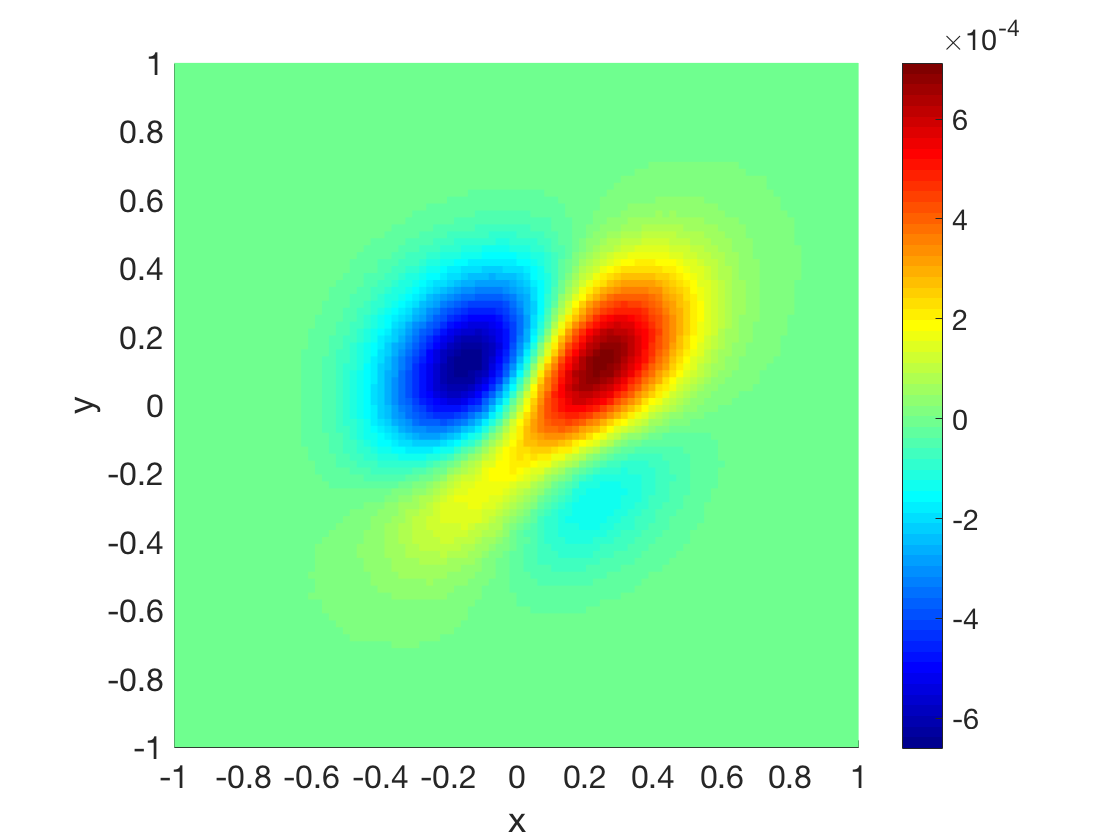
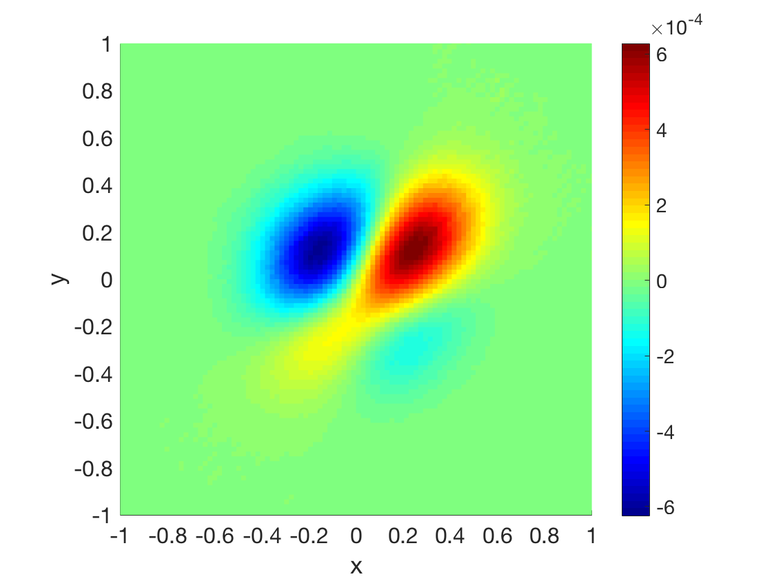
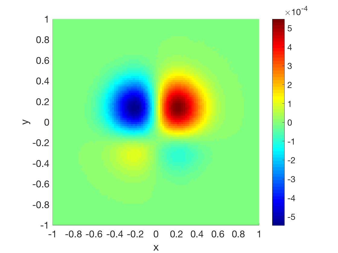
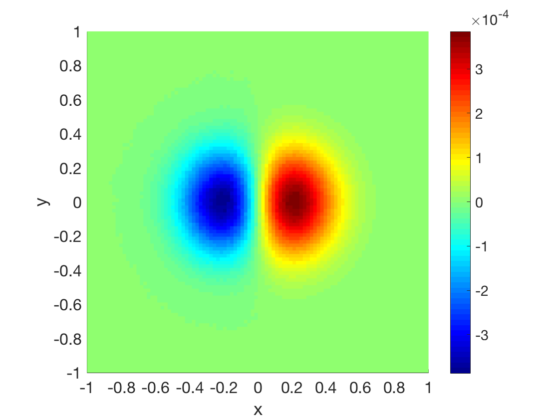
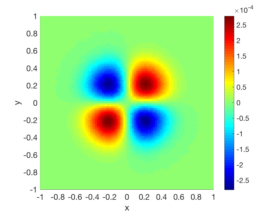
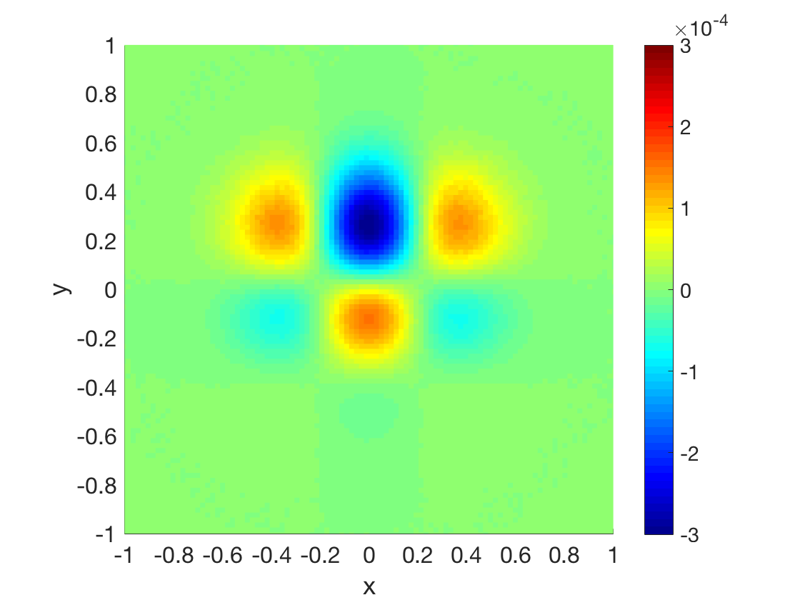
A good compromise was found provided that the resolution was high enough. On Fig. 1, we see that the predicted response was well approximated. This is checked on Table 1 where we show that the error of approximating the perturbed invariant measure using the response formulas in Eq. (21) presented earlier is small. The linear response (see Fig. 2) is precisely doing what one expects: mass is pumped to the right as a consequence of the mean being shifted and the introduction of correlations inflicts a rotation. Higher order correction terms (see Fig. 2) can also give an insight on how the measure is gradually modified. As a safety check, the sum of the components of the response are checked to add up to (almost) zero, meaning that mass is not introduced or depleted.

Figure 1: Response of the O-U to the perturbations considered in Eq. (33). The left-hand figure shows the true response calculated by subtracting the unperturbed invariant measure from the perturbed one. The figure on the right is the predicted response calculated from Eq. (20).

Figure 2: The top-left figure shows the linear response of the O-U process with respect to the perturbations considered in Eq. (33) calculated by truncating Eq. (21) at the first order. The top-right and bottom-left show the linear response to changes in $\epsilon_{1}$ and $\epsilon_{2}$ respectively. The bottom-right figure contains the second order correction obtained via Eq. (21).

Table 1: The first row refers to the values obtained from integrating the O-U process. The rest of the rows are values obtained via discretisation of the transfer operator. We defined Error1 as the $L^{2}$ norm of the difference between the coarse-grained perturbed invariant measure and the first order correction. Error2 is the same but with higher order correction terms.

	$\langle x\rangle$	$\delta_{\epsilon_{1}}\left[x\right]_{1}$	$\delta_{\epsilon_{2}}\left[x\right]_{1}$	Error1	Error2
O-U	0	1	0	0	0
$N=10$	$10^{-4}$	0.47	$3\times 10^{-3}$	0.02	0.02
$N=12$	$10^{-4}$	0.77	$2\times 10^{-3}$	7$\times 10^{-3}$	$5\times 10^{-3}$
$N=14$	$10^{-4}$	0.93	$8\times 10^{-4}$	3$\times 10^{-3}$	$8\times 10^{-4}$

III.3 A Deterministic Dynamical System

A model of importance in dynamical systems and climatology is the Lorenz 63 systemLorenz (1963). Such system is a low-dimensional model of atmospheric convention that, even if it is far from being a realistic model, it possesses chaotic behaviour and exhibits different regimes, just as in the atmosphere. This systems has been the toy-model to illustrate the difficulty of calculating the sensitivity and response in dynamical systems and in the climate system by extension (e.g. Refs. Lea, Allen, and Haine, 2000; Wang, 2013).

From the point of view of the transfer operator, the response of the Lorenz 63 system was computed in Ref. Lucarini, 2016, by means of applying the perturbation theory for finite-state space Markov chains. However, the perturbed dynamics needed to be sampled. In case of low-dimensional models, this is not a major handicap, but in physically relevant systems this can be an expensive procedure. Therefore, we need more predictive skill.

The Lorenz 63 system is a deterministic dynamical system that is given by the following set of ordinary differential equations:

$$\dot{\mathbf{x}}(t)=\mathbf{F}(\mathbf{x})=\begin{cases}&s(y-x)\\ &x(r-z)-y\\ &xy-bz\end{cases},$$ (38)

for the classical parameter values $s=10$, $b=8/3$ and control parameter $r=28$. For such parameter values, the Lorenz 63 system displays chaotic dynamics in a singularly hyperbolic attractor that supports an SRB measureTucker (2002). The lack of uniform hyperbolicity implies that the Lorenz 63 system is not Axiom A and therefore one cannot expect response theory to hold. Nevertheless, numerical evidence supports the idea of linearReick (2002) and nonlinearLucarini (2009) response to be valid in this system.

The perturbation problem we tackle here is that of changing the value of the control parameter $r\rightarrow r+\epsilon_{1}$ for $\epsilon_{1}\in\mathbb{R}$. This parameter is known as the Rayleigh number and it is proportional to the temperature difference between the convecting layers. The bifurcations associated to this parameter are numerically surveyed in Ref. Sparrow, 1982. We would also study the additive perturbation on the $z$-variable by adding $\epsilon_{2}\in\mathbb{R}$. These perturbations incur a modification on the vector field of the form:

$$\dot{\mathbf{x}}(t)=\mathbf{F}(\mathbf{x})+\epsilon_{1}\mathbf{G}_{1}(\mathbf{x})+\epsilon_{2}\mathbf{G}_{2}(\mathbf{x}).$$ (39)

where $\mathbf{G}_{1}(\mathbf{x})=[0,x,0]^{\prime}$ and $\mathbf{G}_{2}(\mathbf{x})=[0,0,1]^{\prime}$. Consequently, the Liouville equation changes as in Eq. (4), with perturbation operators:

$$\mathcal{B}_{1}\rho(\mathbf{x},t)=-\nabla\cdot\left(\mathbf{G}_{1}(\mathbf{x})\rho(\mathbf{x},t)\right)\\$$ (40)

and

$$\mathcal{B}_{2}\rho(\mathbf{x},t)=-\nabla\cdot\left(\mathbf{G}_{2}(\mathbf{x})\rho(\mathbf{x},t)\right).$$ (41)

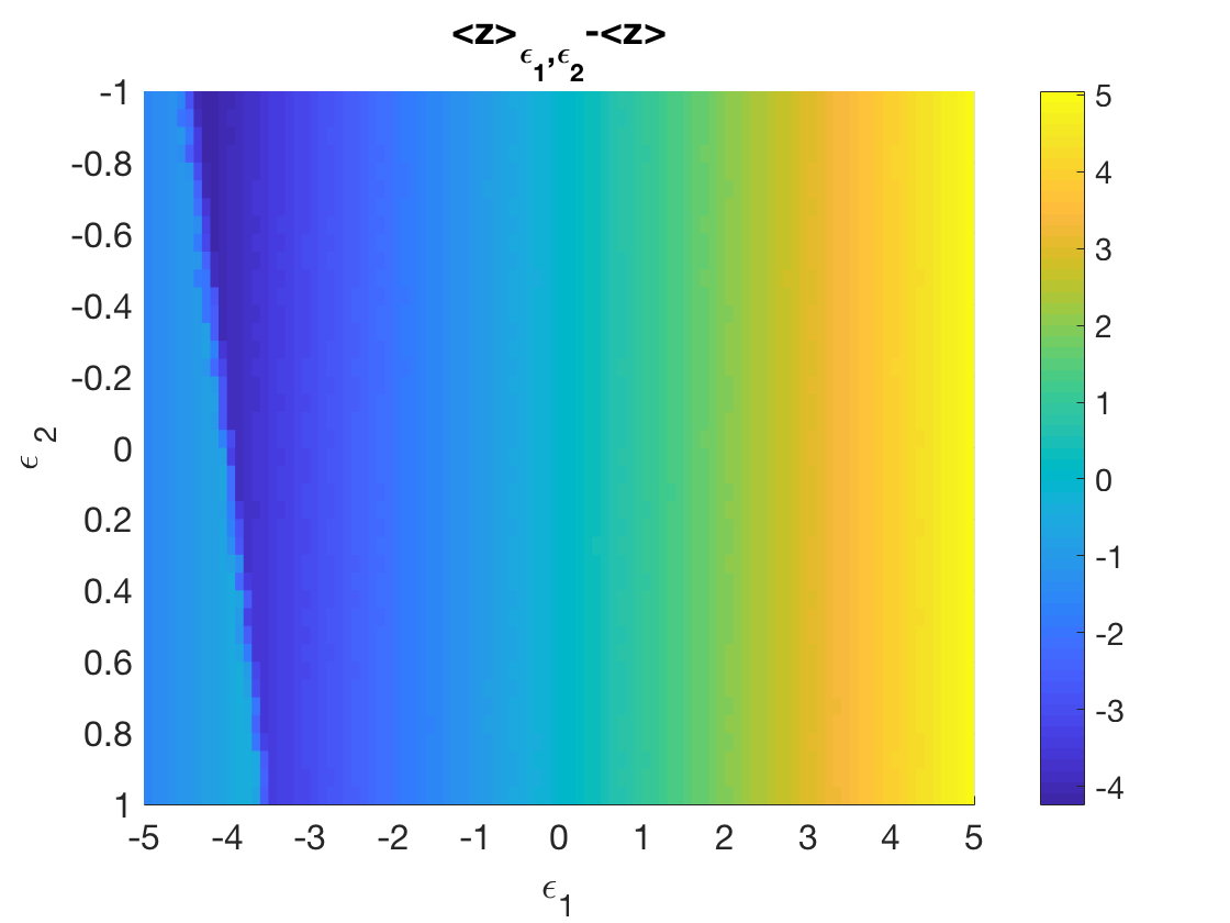
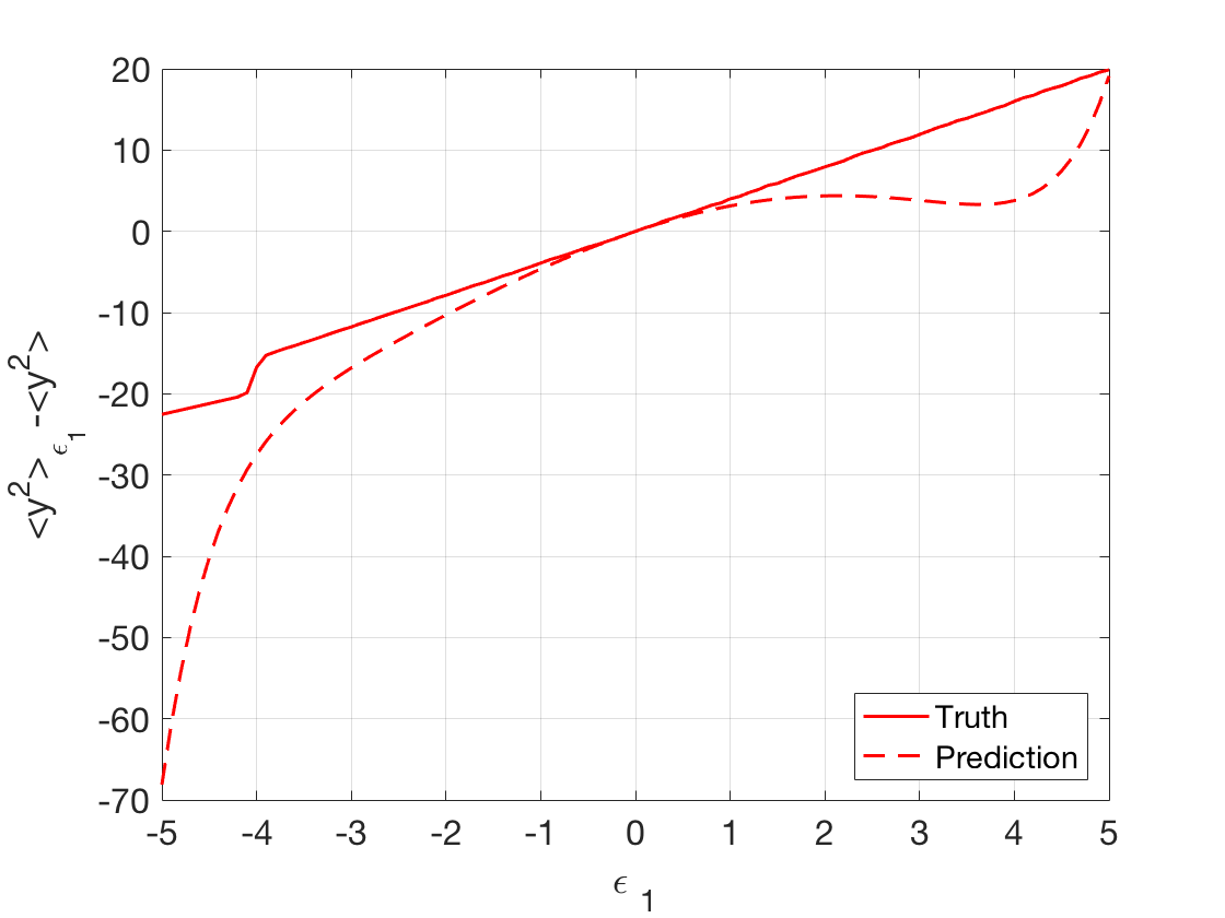
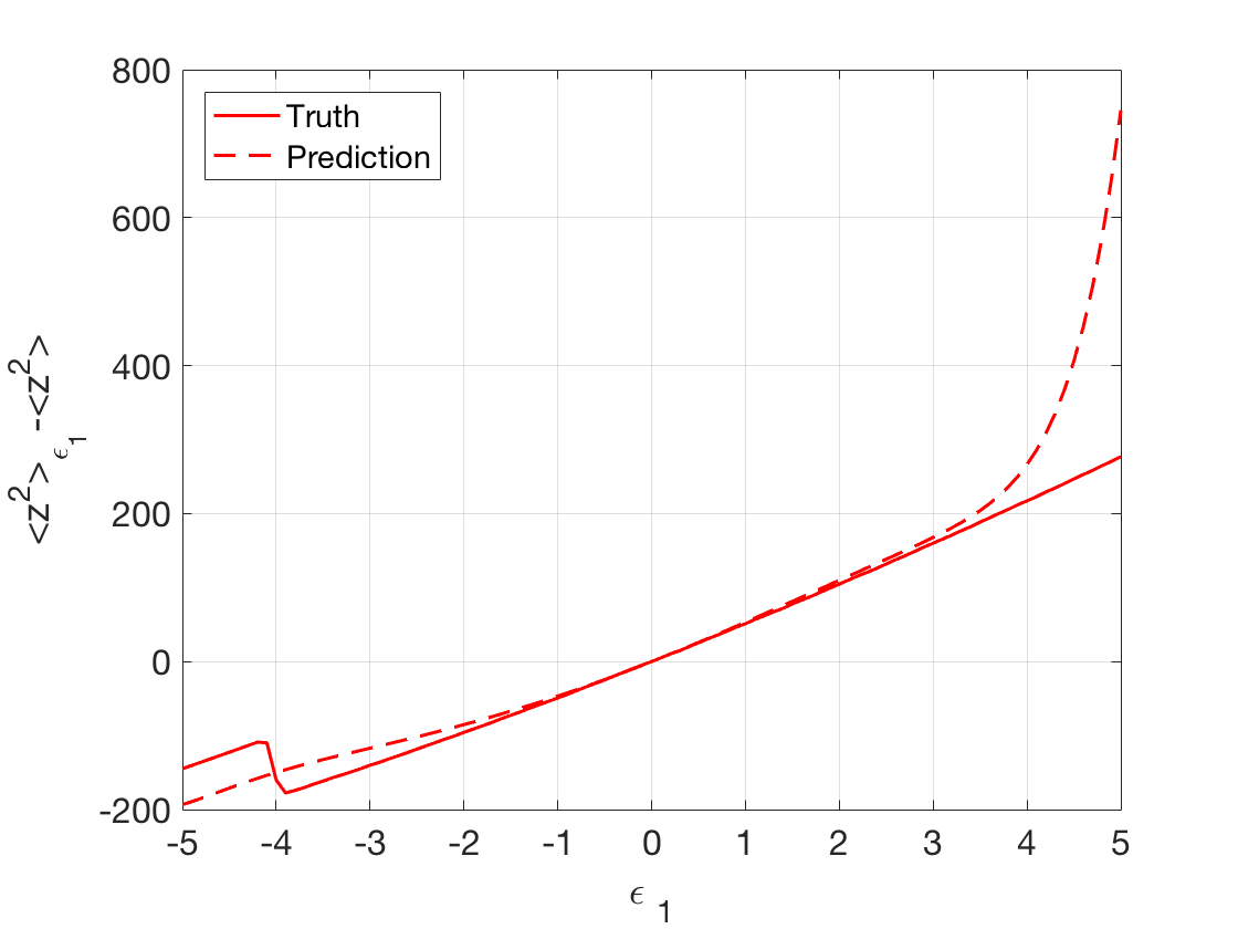
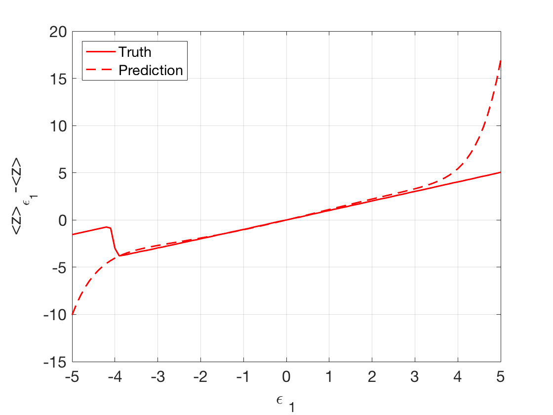
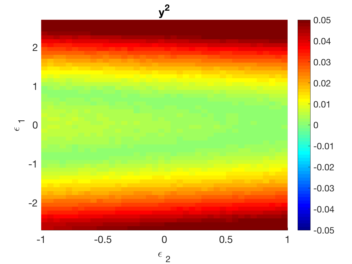
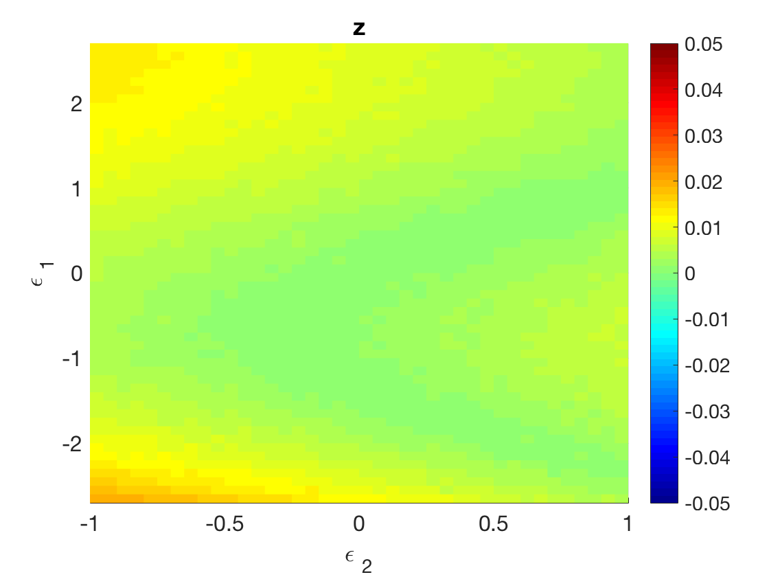
Introducing forcing provokes a change in the statistics of the system as shown on Fig. 3, where we considered the example observable $z$ and computed its mean value for equispaced values of $\epsilon_{1}\in[-5,5]$ and $\epsilon_{2}\in[-1,1]$. When $\epsilon_{1}\approx-4$, a bifurcation is traversed producing a non-smooth change in the mean value of the observable. Far away from this bifurcation point, the statistics changes smoothly with respect to $\epsilon_{1}$ and $\epsilon_{2}$. For the calculation of these means, long integrations were considered so that the outcome is uniquely determined. This is possible thanks to the existence of an SRB measureLea, Allen, and Haine (2000).

Notice that differentiating Eq. (7) with respect to $\epsilon_{k}$ ($k=1,2$) gives $\mathcal{B}_{k}$. So a way of obtaining a matrix representation of $\mathcal{B}_{k}$ is

$$\epsilon_{k}m_{k}=\mathcal{M}_{\epsilon_{k}}^{dt}-\mathcal{M}^{dt}.$$ (42)

Where $\mathcal{M}_{\epsilon_{k}}^{dt}$ is the transition matrix empirically constructed from the perturbed equations. This approach was followed previouslyLucarini (2016) and served to calculate the linear response of the Lorenz 63 system, however, it involves two (or more) long integrations of the equations, something we want to avoid. We explain the methodology carried out here in the next section.

Figure 3: Deviation of perturbed expected values of the observable $z$ for $\epsilon_{1}\in[-5,5]$ and $\epsilon_{2}\in[-1,1]$. The expectation values were computed by integrating the equations for $10^{3}$ time-units with 20 ensemble members for each value of $\epsilon_{1}$ and $\epsilon_{2}$.

Numerics: transition and perturbation matrices

The invariant measure of the Lorenz 63 system is supported on attractor, which by definition is compact. Since we know that the Lorenz attractor is contained in an absorbing closed ellipsoid on phase-spaceSparrow (1982), we are certain that the square defined by the Cartesian product $[-20,20]\times[-30,30]\times[0,50]$ will contain the attractor. Then, to obtain the box partition, we divide into two each axis and repeat the procedure in each resulting segment. This way, a total of $2^{N}$ boxes $\{B_{i}\}_{i=1}^{2^{N}}$ were constructed for the values of $N=12,15$ and $18$. As mentioned earlier, the box discretisation was carried out using GAIODellnitz, Froyland, and Junge (2001).

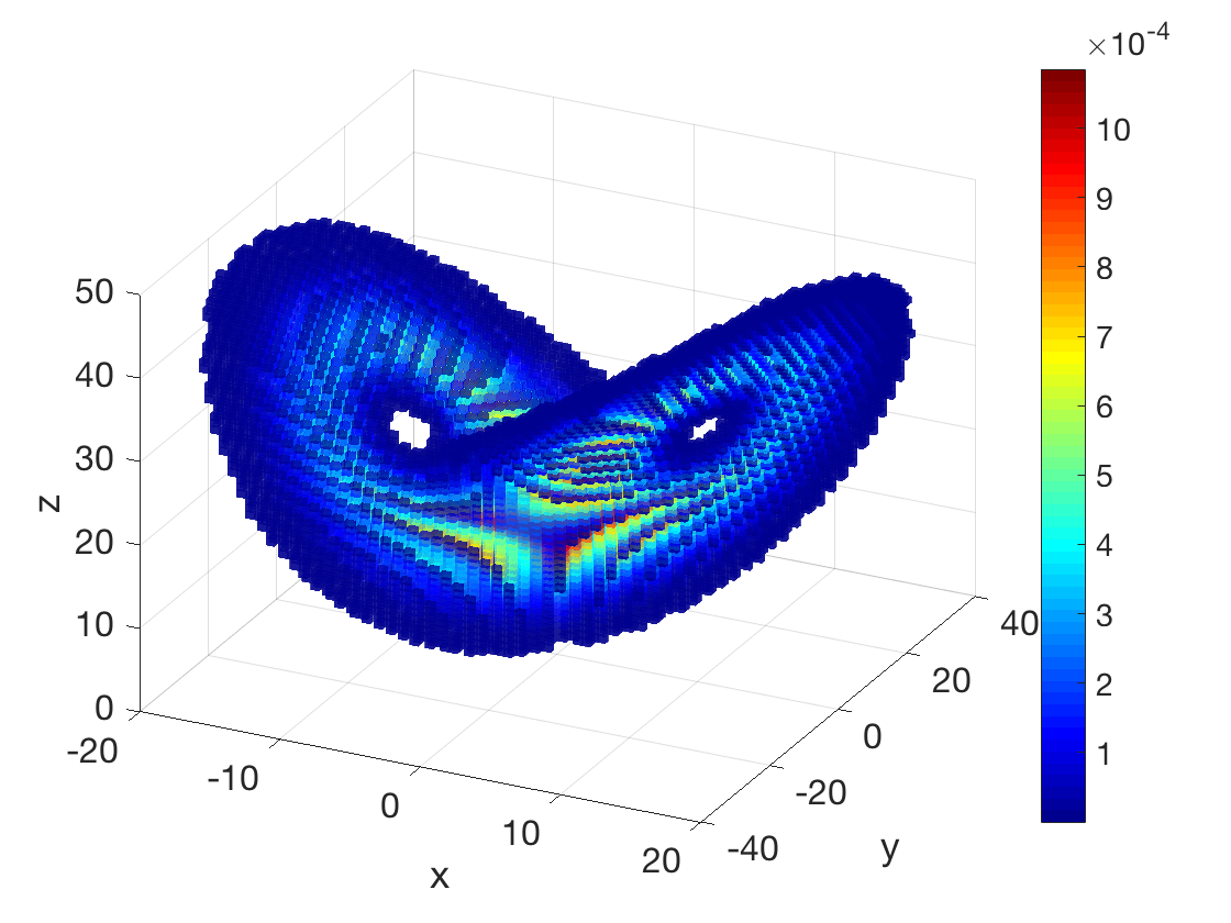
To obtain the sample points of the dynamics, we integrated the model for $10^{5}$ time-units with a time-step of $dt=10^{-3}$ time-units. After a spinup of ten percent of the points, we count the transitions between the boxes with a time-lag of $dt$ time-units. This gives the transition matrix $\mathcal{M}^{dt}$. Thus, a coarse-grained estimation of the invariant measure can be readily obtained by solving the eigenvalue problem in Eq. (11) which is plotted on Fig. 4.

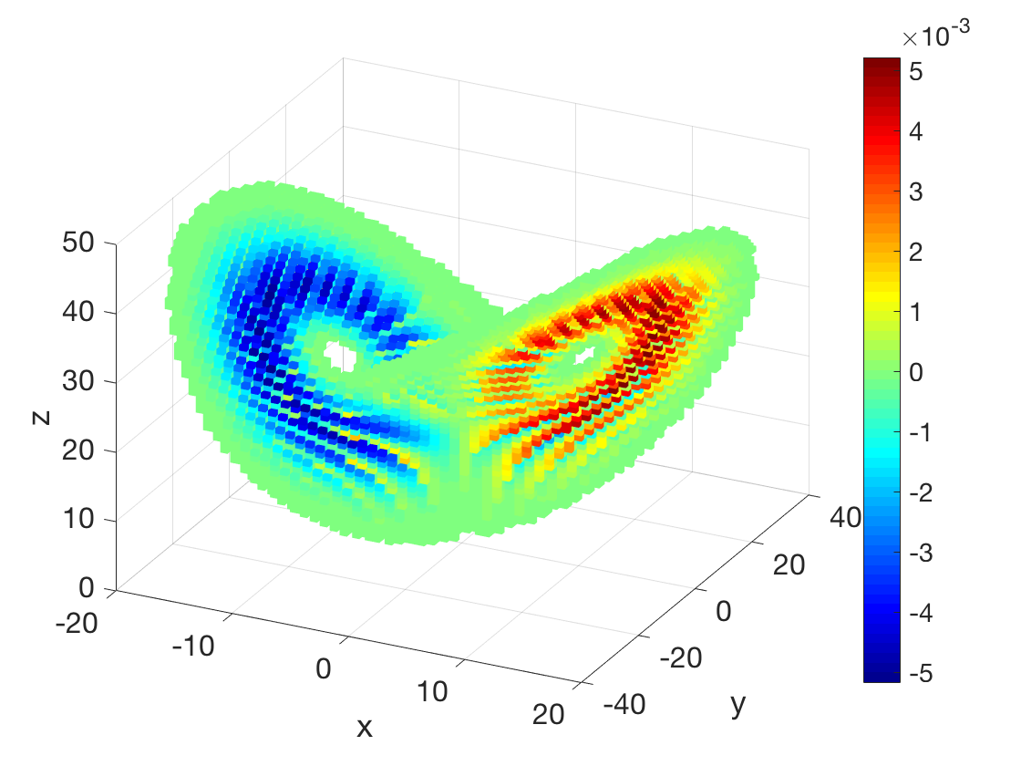
Regarding the perturbation operators, the same techniques as in the O-U process where employed. The difference here is that we are dealing with an invariant measure that is singular with respect to the Lebesgue measure and therefore is supported in a complicated set, as illustrated by Fig. 4. Hence, one needs to take care of the boundary boxes by simply considering forward/backward approximations of the derivatives at those boxes. Thus was estimated $\mathcal{B}_{1}$ applied to the invariant measure, depicted on the right of Fig. 4.

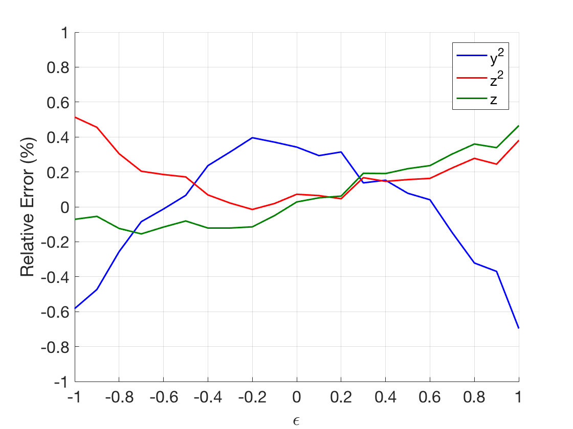
The results of applying this methodology are presented in Fig. 5, where we show that Eq. (21) can indeed approximate the expectation values certain observables for a wide range of values of $\epsilon_{1}$. We underline that these plots demonstrate the validity of the formulae not only to compute the linear response but to predict the statistics of the system. As is natural, the formulas cannot be expected to work for large values of the perturbation parameter, let alone beyond the bifurcation point. When considering the simultaneous forcings $\epsilon_{1}\mathbf{G}_{1}$ and $\epsilon_{2}\mathbf{G}_{2}$, we examine the efficiency of the formulas (Table 2). We calculate the expectation value of certain observables and check that we can approximate their mean for small values of $\epsilon_{1}$ and $\epsilon_{2}$. Also, the linear response is calculated. As we see in the last row, refining the resolution does not always improve the results. This is due to the fact that the length of the integration has to be severely extended in order to sample the boxes covering the domain. In general, the skill of the methodology is shown in Fig. 6 where the expectation values of some observables are predicted using the response formula Eq. (21). Of course, the validity was only tested within the convergence interval.

Figure 4: Coarse-grained Lorenz 63 invariant measure (left) and the discretised operator $\mathcal{B}_{1}$ applied onto the invariant measure (right).

Figure 5: Predictions for perturbations on $r$. Mean values of the observables indicated in the panels are predicted using Eq. (21) and plotted against the true means observed empirically via integrations of the system.

Figure 6: Relative error $(\%)$ of the prediction of the expected values of the observables indicated in the plots. The prediction was done by evaluating Eq. (21) and the true values were obtained empirically by integrating the equations for each value of $\epsilon_{1}$ and $\epsilon_{2}$.

Table 2: Expectation values with respect to the unperturbed and perturbed ($\epsilon_{1}=0.1$ and $\epsilon_{2}=0.1$) invariant measure. In the first row time averages were used whereas the rest indicate the expection values obtained by means of evaluating Eq. (20) with a transition matrix of size $N\times N$.

	$\langle y^{2}\rangle$	$\langle z\rangle$	$\langle y^{2}\rangle_{\epsilon_{1},\epsilon_{2}}$	$\langle z\rangle_{\epsilon_{1},\epsilon_{2}}$	$\delta_{\epsilon_{1}}\left[y^{2}\right]_{1}$	$\delta_{\epsilon_{1}}\left[z\right]_{1}$	$\delta_{\epsilon_{2}}\left[y^{2}\right]_{1}$	$\delta_{\epsilon_{2}}\left[z\right]_{1}$
L-63	81.20	23.54	81.44	23.65	3.95	1.01	-1.47	0
$N=12$	82.37	23.55	82.50	23.62	3.01	0.89	-1.65	-0.14
$N=15$	81.48	23.55	81.70	23.65	3.97	1.08	-1.62	-0.11
$N=18$	81.25	23.55	81.30	23.65	2.68	1.11	-1.57	-0.09

IV Discussion

In this work, we take the point of view of statistics to understand the effect of perturbations on dynamical systems. Under this setting, the transfer operator is the essential object of study. By means of projecting such operator onto a finite dimensional vector space, it is possible to obtain empirically constructed matrix representations of the transfer operator via Markov modelling. Further, the properties of these matrices allow us to, up to finite precision, describe the dynamical system of interest.

Exploiting the stochastic (or Markovian) structure of the projected transfer operator, we consider multiple perturbations and express the resulting perturbed invariant measure as a series expansion describing the response at all orders of nonlinearity. Alongside previous workSchweitzer (1968); Lucarini (2016); Froyland, Antown, and Cevi (2018), it is possible to link the probabilistic concepts of finite Markov chains to dynamical systems. Namely, the mixing rate of the unperturbed chain indicated by its second eigenvalue or more generally its ergodicity coefficient determine the validity of the perturbative expansions. This agrees with more theoretical considerations with the so-called spectral gap conditionHairer and Majda (2010), key to establish linear response.

The linear component in the perturbative expansion is the so called linear response and it is of physical interestMarconi et al. (2008). This quantity is accessed by constructing suitable response operators and indicates the sensitivity of a dynamical system to prescribed perturbations. Here we emphasize the need of gaining predictive skill: given a perturbation to the vector field (possibly induced by tuning several paramters), can we calculate the sensitivity of the system a priori? For such purpose, we examined the Fokker-Planck/Liouville equation to identify the operators that incur the perturbations on the evolution of densities. Then, by considering simple finite-difference methods, we were able to model (to finite-precision) matrix perturbations that allowed to exploit the perturbative formulas giving us access to the linear and nonlinear response of the systems. Notice that using this method, we only need one integration of the (unforced) model to determine the response and sensitivity.

The two numerical experiments performed were intrinsically different. The Ornstein-Uhlenbeck process is a stochastic dynamical system with an invariant measure with a density (with respect to the Lebesgue measure) which is smooth. Therefore, differential operators (discretised using finite-differences) should work correctly. On the other hand, the Lorenz 63 model is a dissipative deterministic system with an attractor with Lebesgue-zero measure that is singularly hyperbolic. This translates into the fact that linear response theory is not theoretically provedRuelle (2009). Moreover, the invariant measure of such system is not smooth, so the usual notion of differentiation does not hold. In the experiments, we coarse-grained the invariant measure to obtain a vector estimate. The corresponding differential operators were applied giving a good compromise, suggesting that at a coarse-grained level, the usual methods for numerical differentiation should work. Previous investigationsFroyland, Junge, and Koltai (2013) illustrate that coarse-graining the domain inherently provokes the introduction numerical diffusion thus smoothening the invariant measure.

The partitioning of phase-space is an arbitrary decision of the modeller. In these numerical experiments, the partitioning is considered to be uniform: boxes are of equal size. This is not optimal, since there might be regions of phase-space that need more refining than othersDellnitz and Junge (1999); Froyland (2001). The reason for choosing equally sized boxes is that the invariant measures obtained gave a good compromise when approximating the expectation value of observables. In any case, comparing box discretisations is not the target of the paper.

The low dimensionality of the problems considered in this paper allows to perform the box subdivision on the whole phase-space. Unfortunately, many physically relevant models posses a domain which is high-dimensional not to say infinite-dimensional. In these cases, it appears intractable to work on the complete domain. Because of this dimensionality barrier, reduced phase-spaces are considered. Results along this line support the applicability of the transfer operator methods in a climatological context, see, e.g., Refs. Chekroun et al., 2014; Tantet, van der Burgt, and Dijkstra, 2015; Tantet et al., 2018. However, the inherent loss of Markovianity in the dimensionality reduction requires control on the memory effects introduced by the hidden variables (see, e.g., Ref. Kondrashov, Chekroun, and Ghil, 2015), something that complicates the study of the response, as pointed out in Ref. Lucarini and Wouters, 2017 where the robustness of reduced systems with the presence of forcing is assessed. Further research should be oriented on adapting this methodology based on the transfer operator in higher-dimensional systems with vistas to assessing and predicting the sensitivity of physically relevant systems.

References

- Marconi et al. (2008) U. M. B. Marconi, A. Puglisi, L. Rondoni, and A. Vulpiani, “Fluctuation-Dissipation: Response Theory in Statistical Physics,” Physics Reports 461 (2008).
- Lasota and Mackey (1994) A. Lasota and M. C. Mackey, Chaos, fractals and noise (Springer, New York, 1994).
- Kubo (1957) R. Kubo, “Statistical-mechanical theory of irreversible processes I,” Journal of the Physical Society of Japan 12, 570–586 (1957).
- Ruelle (1997) D. Ruelle, “Differentiation of SRB states,” Communications in Mathematical Physics 187, 227–241 (1997).
- Ruelle (2009) D. Ruelle, “A review of linear response theory for general differentiable dynamical systems,” Nonlinearity 22, 855–870 (2009).
- Eckmann and Ruelle (1985) J. P. Eckmann and D. Ruelle, “Ergodic theory of chaos and strange attractors,” Reviews of Modern Physics 57, 617–656 (1985).
- Abramov and Majda (2007) R. V. Abramov and A. J. Majda, “Blended response algorithms for linear fluctuation-dissipation for complex nonlinear dynamical systems,” Nonlinearity 20, 2793–2821 (2007).
- Gritsun and Lucarini (2017) A. Gritsun and V. Lucarini, “Fluctuations, response, and resonances in a simple atmospheric model,” Physica D: Nonlinear Phenomena 349, 62–76 (2017).
- Ragone, Lucarini, and Lunkeit (2016) F. Ragone, V. Lucarini, and F. Lunkeit, “A new framework for climate sensitivity and prediction : a modelling perspective,” Climate Dynamics 46, 1459–1471 (2016).
- Lucarini, Lunkeit, and Ragone (2017) V. Lucarini, F. Lunkeit, and F. Ragone, “Predicting Climate Change Using Response Theory : Global Averages and Spatial Patterns,” Journal of Statistical Physics 166, 1036–1064 (2017).
- Baladi (2000) V. Baladi, Positive Transfer Operators and Decay of Correlations (World Scientific, Singapore, 2000).
- Engel and Nagel (2006) K.-J. Engel and R. Nagel, A Short Course on Operator Semigroups (Springer, 2006).
- Risken (1989) H. Risken, The Fokker-Planck Equation, 2nd ed. (Springer, 1989).
- Tantet et al. (2018) A. Tantet, V. Lucarini, F. Lunkeit, and H. A. Dijkstra, “Crisis of the chaotic attractor of a climate model : a transfer operator approach,” Nonlinearity 31, 2221–2251 (2018).
- Tantet, van der Burgt, and Dijkstra (2015) A. Tantet, F. R. van der Burgt, and H. A. Dijkstra, “An early warning indicator for atmospheric blocking events using transfer operators,” Chaos 25, 036406 (2015).
- Froyland et al. (2007) G. Froyland, K. Padberg, M. H. England, and A. M. Treguier, “Detection of coherent oceanic structures via transfer operators,” Physical Review Letters 98, 1–4 (2007).
- Tantet, Lucarini, and Dijkstra (2018) A. Tantet, V. Lucarini, and H. A. Dijkstra, “Resonances in a Chaotic Attractor Crisis of the Lorenz Flow,” Journal of Statistical Physics 170, 584–616 (2018).
- Lucarini (2016) V. Lucarini, “Response Operators for Markov Processes in a Finite State Space: Radius of Convergence and Link to the Response Theory for Axiom A Systems,” Journal of Statistical Physics 162, 312–333 (2016).
- Froyland, Antown, and Cevi (2018) G. Froyland, F. Antown, and D. D. Cevi, “Optimal linear responses for markov chains and stochastically perturbed dynamical systems,” Journal of Statistical Physics 170, 1051–1087 (2018).
- Seneta (1973) E. Seneta, Non-negative matrices (George Allen and Unwin, 1973).
- Schweitzer (1968) P. J. Schweitzer, “Perturbation Theory and Finite Markov Chains,” Journal of Applied Probability 5, 401–413 (1968).
- Funderlic and Meyer (1986) R. E. Funderlic and C. D. Meyer, “Sensitivity of the stationary distribution vector for an ergodic Markov chain,” Linear Algebra and Its Applications 76, 1–17 (1986).
- Seneta (1979) E. Seneta, “Coefficients of Ergodicity : Structure and Applications,” Applied Probability Trust 11, 576–590 (1979).
- Seneta (1993) E. Seneta, “Sensitivity of finite Markov chains under perturbation,” Statistics and Probability Letters 17, 163–168 (1993).
- Inubushi (2019) M. Inubushi, “Unpredictability and robustness of chaotic dynamics for physical random number generation,” Chaos 29, 033133 (2019).
- Mitrophanov (2003) A. Y. Mitrophanov, “Stability and Exponential Convergence of Continuous-Time Markov Chains,” Applied Probability Trust 40, 970–979 (2003).
- Bauer and Fike (1960) F. L. Bauer and C. T. Fike, “Norms and Exclusion Theorems,” Numerische Mathematik 2, 137–141 (1960).
- Wilkinson (1965) J. H. Wilkinson, The Algebraic Eigenvalue Problem (Oxford University Press, 1965).
- Robinson (2001) J. C. Robinson, Infinite Dimensional Dynamical Systems (Cambridge University Press, 2001).
- Da Prato and Zabczyk (1996) G. Da Prato and J. Zabczyk, Ergodicity for Infinite Dimensional Systems (Cambridge University Press, 1996).
- Dellnitz, Froyland, and Junge (2001) M. Dellnitz, G. Froyland, and O. Junge, “The algorithms behaind GAIO-set oriented numerical methods for dynamical systems,” in Ergodic theory, analysis, and efficient simulation of dynamical systems (Springer, Berlin, 2001) pp. 145–174.
- Froyland, Junge, and Koltai (2013) G. Froyland, O. Junge, and P. Koltai, “Estimating long term behavior of flows without trajectory integration: the infinitesimal generator approach,” SIAM J. Numerical Analysis 51, 223–247 (2013).
- Lorenz (1963) E. N. Lorenz, “Deterministic Nonperiodic Flow,” Journal of the Atmospheric Sciences 20, 130–141 (1963).
- Lea, Allen, and Haine (2000) D. J. Lea, M. R. Allen, and T. W. N. Haine, “Sensitivity analysis of the climate of a chaotic system,” Tellus 52, 523–532 (2000).
- Wang (2013) Q. Wang, “Forward and adjoint sensitivity computation of chaotic dynamical systems,” Journal of Computational Physics 235, 1–13 (2013).
- Tucker (2002) W. Tucker, “A Rigorous ODE Solver and Smale ’ s 14th Problem,” Foundations of Computational Mathematics 2, 53–117 (2002).
- Reick (2002) C. H. Reick, “Linear response of the Lorenz system,” Physical Review E 66, 036103 (2002).
- Lucarini (2009) V. Lucarini, “Evidence of dispersion relations for the nonlinear response of the Lorenz 63 system,” Journal of Statistical Physics 134, 381–400 (2009).
- Sparrow (1982) C. Sparrow, The Lorenz Equations (Springer, 1982).
- Hairer and Majda (2010) M. Hairer and A. J. Majda, “A simple framework to justify linear response theory,” Nonlinearity 23, 909–922 (2010).
- Dellnitz and Junge (1999) M. Dellnitz and O. Junge, “On the approximation of complicated behaviour,” SIAM J. Numerical Analysis 36, 491–515 (1999).
- Froyland (2001) G. Froyland, “Extracting dynamical behaviour via Markov models,” in Nonlinear Dynamics and Statistics (Birkhäuser, Boston, MA, 2001).
- Chekroun et al. (2014) M. Chekroun, J. D. Neelin, D. Kondrashov, J. C. McWilliams, and M. Ghil, “Rough parameter dependence in climate models and the role of ruelle-pollicot resonances,” Proceedings of the National Academy of Sciences of the United States of America 111, 1684–1690 (2014).
- Kondrashov, Chekroun, and Ghil (2015) D. Kondrashov, M. D. Chekroun, and M. Ghil, “Data-driven non-Markovian closure models,” Physica D 297, 33–55 (2015).
- Lucarini and Wouters (2017) V. Lucarini and J. Wouters, “Response formulae for n-point correlations in statistical mechanical systems and application to a problem of coarse graining,” Journal of Physics A: Mathematical and Theoretical 50, 355003 (2017).
- Seneta (1984) E. Seneta, “Explicit Forms for Ergodicity Coefficients,” Linear Algebra and Its Applications 60, 187–197 (1984).
- C. E. Leith (1975) C. E. Leith, “Climate Response and Fluctuation Dissipation,” Journal of the Atmospheric Sciences 32, 2022–2026 (1975).
- Mitrophanov (2005) A. Y. Mitrophanov, “Sensitivity and Convergence of Uniformly Ergodic Markov Chains,” Applied Probability Trust 42, 1003–1014 (2005).
- Froyland (1998) G. Froyland, “Approximating physical invariant measures of mixing dynamical systems in higher dimensions,” Nonlinear Analysis 32, 831–860 (1998).
- Ipsen and Selee (2014) I. C. F. Ipsen and T. Selee, “Ergodicity Coefficients Defined by Vector Norms,” SIAM Journal on Matrix Analysis and Applications 32, 153–200 (2014).
- Gouëzel and Liverani (2006) S. Gouëzel and C. Liverani, “Banach spaces adapted to Anosov systems,” Ergodic Theory and Dynamical Systems 26, 189–217 (2006).