Dipole evolution: perspectives for collectivity and collisions
Abstract
The transverse, spatial structure of protons is an area revealing fundamental properties of matter, and provides key input for deeper understanding of emerging collective phenomena in high energy collisions of protons, as well as collisions of heavy ions. In this paper eccentricities and eccentricity fluctuations are predicted using the dipole formulation of BFKL evolution. Furthermore, first steps are taken towards generation of fully exclusive final states of collisions, by assessing the importance of colour fluctuations in the initial state. Such steps are crucial for the preparation of event generators for a future electron-ion collider. Due to the connection between an impact parameter picture of the proton structure, and cross sections of and collisions, the model parameters can be fully determined by fits to such quantities, leaving results as real predictions of the model.
Keywords:
QCD, BFKL evolution, Monte Carlo event generators, Flow, Small Systems, Electron-Ion collider1 Introduction
In the research program at the Large Hadron Collider (LHC) and the Relativistic Heavy Ion Collider (RHIC), collisions of ultra relativistic heavy ions are hypothesized to result in the creation of a quark-gluon plasma (QGP) with partonic degrees of freedom. One of the main avenues for investigating and characterizing this plasma consists of measurements of azimuthal correlations between particle pairs separated in rapidity, connecting particle emission angles to the initial geometry of the collision. Non-trivial correlations reflecting collective properties were first observed in gold–gold and copper–copper collisions at RHIC Ackermann:2000tr , but has since been investigated also in lead–lead (PbPb) collisions at the LHC Aamodt:2010pa ; Chatrchyan:2011eka ; ATLAS:2012at . Such non-trivial azimuthal correlations had at that point already been hypothesized to be a signal for hydrodynamic behaviour Ollitrault:1992bk , or, even earlier, to involve microscopic dynamics of overlapping ”quark tubes” or strings Abramovsky:1988zh .
Similar results have been obtained in smaller collision systems such as proton–lead () CMS:2012qk , deuteron–gold Aidala:2017ajz , and, perhaps most surprisingly, in proton–proton () Khachatryan:2010gv . Attempts to observe similar behaviour in even smaller collision systems, e.g. , has, while carrying interesting prospects, so far not produced positive results Badea:2019vey . Even though the discovery of collectivity in is almost ten years old, the origin of such correlations in small collision systems is still highly debated (see ref. Nagle:2018nvi for a recent review), and its resolution is among the top priorities for the future heavy ion program at LHC Citron:2018lsq . One possibility is that the correlations in these small collision systems are due to coherence effects Blok:2017pui or initial state correlations Dusling:2012wy . Another is a repetition of the argument from heavy ion collisions, where the observed collective behaviour is a hydrodynamic response to the initial partonic spatial configuration Weller:2017tsr . A picture where a hydrodynamic “core” coexists with a non-hydrodynamic “corona” has been shown by the EPOS model Werner:2007bf ; Pierog:2013ria to provide good descriptions of collectivity even in small collision systems.
The possibility of a hydrodynamic (or in fact any other) response to an initial geometric configuration of partons, poses a challenge to the traditional strategies for event generators, such as Pythia 8 Sjostrand:2014zea or Herwig 7 Bellm:2015jjp , both based on perturbative QCD (pQCD) with no obvious way to extract a spatial configuration for which to calculate a response. Attempts to calculate such a structure dEnterria:2010xip ; Albacete:2016pmp ; Bierlich:2017vhg generally involve assuming a certain spatial distribution of partons in the proton and, using the eikonal approximation, then transferring this structure to a spatio-temporal structure of the multiple partonic interactions (MPIs). The immediate drawbacks of such an approach are that (a) such models will in general contain parameters which need to be fitted to the same type of particle correlations as they wish to predict, and (b) assuming a spatial distribution of partons in a proton will generally contain many ad hoc elements.
Even though the spatial distribution of partons in a proton cannot be assessed ab initio, the evolution of said distribution can be calculated perturbatively in the formalism of Mueller Mueller:1993rr ; Mueller:1994jq . At high energies, average properties will retain little dependence on the initial configuration, i.e. be mostly dependent on the evolution. Since the transverse substructure of the colliding protons (or virtual photons) can be linked to total or semi-inclusive cross sections, any model parameters can be tuned to such quantities, and leave any further estimation of collective effects as real predictions of the model. Attempts to predict the elliptic flow in collisions using an implementation of Mueller’s model was provided in 2011 Avsar:2010rf , showing comparable to values found from at RHIC and LHC energies.
This paper is concerned with presenting a new Monte Carlo implementation of Mueller’s model, study its description of cross sections in pp and collisions, in order to provide estimates on parton level geometries in , proton–ion () and ion–ion () collisions, linked to collective phenomena. Mueller’s model has been implemented as a Monte Carlo several times before, as it is not only useful for calculating spatial distributions of partons, but in fact has much wider applications due to the equivalence of the Mueller formalism with B-JIMWLK (Balitsky, Jalilian-Marian, Iancu, McLerran, Weigert, Leonidov and Kovner) Balitsky:1995ub ; Balitsky:1998kc ; Balitsky:2001re ; JalilianMarian:1997jx ; JalilianMarian:1997gr ; Iancu:2001ad ; Iancu:2000hn ; Weigert:2000gi evolution (see section 2). Such an implementation makes direct introduction of effects beyond the leading logarithmic approximation possible, e.g. conservation of energy and momentum without imposing kinematical constraints on the splitting kernel Deak:2019wms . This makes the implementation attractive for estimation of basic quantities dominated by small processes (e.g. cross sections) in cases where little guidance from data exists. In this paper (see section 7) we will also apply the formalism to extract Glauber–Gribov (GG) colour fluctuations in collisions, in order to take the initial steps towards a generation of electron–ion () collisions within the Angantyr framework Bierlich:2016smv ; Bierlich:2018xfw – a possibility which is foreseen to aid the preparation of an program currently being planned Accardi:2012qut .
Earlier implementations of the Mueller dipole model include the public Oedipus Salam:1996nb and Dipsy Avsar:2005iz ; Flensburg:2011kk codes, as well as a private implementation by Kovalenko et al. Kovalenko:2012ye . All implementations treat only gluons in the evolution, as will this work. The implementation in this paper is similar to the implementation in Dipsy in some respects, but differs in other, while bearing less resemblance to the other two. The key differences between most of the used approaches, lies in the treatment of effects beyond leading order. Worth mentioning already here, is the treatment of sub-leading (number of colours) effects in the evolution, leading to saturation in the cascade. In Dipsy, this is addressed through so-called swing mechanisms Avsar:2007xg ; Avsar:2007xh , which suppresses the contribution from large dipoles in dense environments by replacing them with small dipoles. In this paper we consider only sub-leading effects in the collision frame, by including multiple interactions in a way consistent with unitarity. Thus we make no attempt at treating saturation in the cascade, as the focus is rather to study how well one can do with an approach that includes only a minimal set of sub-leading corrections. Effects included in this paper is energy-momentum conservation and recoil effects (which are beyond leading log) and confinement (which is a non-perturbative effect). This also separates our approach from the IP-Glasma approach Schenke:2012wb , which includes gluon saturation effects in the initial configuration explicitly, and evolve using B-JIMWLK.
On a more technical note, the approach presented in this paper is implemented within the larger framework of the Pythia 8 Monte Carlo event generator. This first of all means that the implementation will become publicly available,111From a future version of Pythia, larger than version 8.300, yet to be determined. See https://home.thep.lu.se/Pythia for up-to-date information. and to aid reproducibility and transparency, a large part of the manuscript, as well as appendix A, are devoted to the details of the implemented model. Our approach is simplistic in the sense that only a minimal amount of corrections to Mueller’s original model has been added, and where ambiguities have arisen, the simplest possible choice has been taken.
The structure of the paper is as follows: After this introduction, the pQCD model of Mueller is introduced. Then follows a description on how observables are calculated within the Good-Walker framework as well as a definition of the observables related to the substructure of protons. The next section describes the overall features of the Monte Carlo implementation, before we proceed to the results on cross sections, eccentricities and colour fluctuations in processes with incoming virtual photons. Lastly, a section is devoted to conclusions and forthcoming work.
2 Proton substructure evolution
In this section we will outline the theoretical basis of the initial state evolution approach used in subsequent sections, and briefly review its relation to other approaches. The theoretical basis is the well known dipole QCD model by Mueller et al. Mueller:1993rr ; Mueller:1994jq .
2.1 Dipole evolution in impact parameter space
We consider in general a picture with a projectile with a dipole structure incident on a target. In the simplest case, the projectile is just a single dipole , spanned between the coordinates and , in impact parameter space. The probability at leading order for this dipole to branch when evolved in rapidity (), is
| (1) |
Here is the transverse coordinate of the emitted gluon and is used as a short-hand for the splitting kernel. An observable known initially, will after an infinitesimal interval have the expectation value (denoted by a bar), assuming unitarity:
| (2) |
where denotes the evaluation of the observable in the two dipole system . In the limit this becomes:
| (3) |
Remarkably, eq. (3) allows for the evolution of any observable calculable in impact parameter space. In the case of -matrices in impact parameter space, the evaluation in the two dipole system reduces to a normal product in the eikonal approximation. Thus . Changing to scattering amplitudes, , by substituting , one obtains:
| (4) |
This is the B-JIMWLK equation hierarchy Balitsky:1995ub ; Balitsky:1998kc ; Balitsky:2001re ; JalilianMarian:1997jx ; JalilianMarian:1997gr ; Iancu:2001ad ; Iancu:2000hn ; Weigert:2000gi in impact parameter space, which, as shown already by Mueller Mueller:2001uk , can be generated directly from eq. (1). Equation (4) includes a non-linear term, , and the treatment of this term is defining for many of the various approaches dealing with initial state evolution at low .
Removal of the non-linear term yields the BFKL (Balitsky, Fadin, Kuraev and Lipatov) equation Kuraev:1977fs ; Balitsky:1978ic , which correctly sums all of the leading logarithms in energy (or, more precisely in rapidity ) to all orders. Other than simply neglecting it, the simplest treatment of the non-linear term is by a mean-field approach, where it factorizes as: . This approximation yields the BK (Balitsky and Kovchegov) equation Kovchegov:1999yj ; Balitsky:1995ub .
2.2 The Mueller dipole model
Several approaches have been proposed to utilize the simple, but powerful evolution equation introduced in eq. (4). Here we will focus on the Mueller dipole model that neglects the non-linear term completely, but is particularly suitable for calculation of geometric quantities. Usually, eq. (4) is solved as an initial value problem: given a scattering matrix at small initial rapidity (), it determines the resulting scattering matrix at any . Note however, that eq. (3) is applicable for any type of observable calculable in impact-parameter space, notably observables linked to the geometry of the partonic initial state. As an example, consider the average vertex coordinate position, , where is either the or coordinate of a dipole. For a single dipole , for the two dipole system , where the two dipoles has a common point , and directly:
| (5) |
For more complicated geometric observables, such as eccentricity (see section 3.2), the analytic expressions become quite involved, and must be handled observable by observable. They are, however, quite easy to handle in a Monte Carlo, where any can be evaluated event by event, and the expectation value extracted from a large statistics sample.

The starting point for the model, is the evolution of an Onium (or ) state in transverse space and rapidity, following eq. (1). Instead of calculating average quantities directly from the evolution equation, Monte Carlo events are generated, by performing a probabilistic evolution of a given initial state, corresponding to a collision event performed by an experiment. The calculational details of performing such an evolution are deferred to section 4 and appendix A. It is, however, important to note here the approximation of this evolution, namely that all dipoles in the dipole-chain radiate independently, removing the non-linear effect from the cascade itself.
After a full evolution in rapidity, a single dipole will have evolved to a chain of dipoles, each of which are allowed to interact with dipoles from another evolved system through gluon exchange. The lowest order interaction between two dipoles, at amplitude level, is single gluon exchange, resulting in two gluon exchange at cross section level. This cross section can be related to the elastic amplitude (cf. section 3.1) through the optical theorem. The dipole-dipole cross section depends on the distances between the interacting dipoles (the enumeration of dipoles follows figure 1) as Kovchegov:2012mbw :
| (6) |
where the arrow indicates that the ’t Hooft large- limit222The ’t Hooft large- limit is the limit where factors of are kept fixed while factors of are suppressed. is taken to reach line 2 of eq. (2.2), which then defines . The ’t Hooft large- limit is taken in order to ensure consistency with the leading logarithmic approximation in the (BFKL) evolution. The distances are indicated in figure 1, except for and , the distances between (anti-)colour-(anti-)colour pairs (1,3) and (2,4). Where the dipole evolution comes with a factor of , the dipole-dipole cross section is proportional to . Thus in the ’t Hooft limit where , the dipole evolution is of order , while the dipole-dipole interaction is of order . This means the dipole-dipole interaction is formally -suppressed compared to the dipole evolution Kovchegov:2012mbw .
A single collision can contain several dipole-dipole scatterings, equivalent to MPIs in a standard parton language. Assuming that the individual scatterings are uncorrelated, the contribution from each scattering exponentiates, resulting in the unitarized scattering amplitude for a single event (see section 3.1):
| (7) |
As each comes with a factor of , the unitarized scattering amplitude correctly resums -suppressed terms in the interaction. In Regge terminology, each scattering can be viewed as a Pomeron exchange. The first term in the expansion corresponds to single Pomeron exchange, and the latter terms to multi-Pomeron exchanges. The unitarized scattering amplitude can thus also be viewed as a resummation of all possible Pomeron exchanges in the collision frame.
An expansion of the exponent in eq. (7) into a power series results in factors of . To second order this results in a term quadratic in , which corresponds to the mean-field approximation of the non-linear term from eq. (4). As this non-linear term corresponds to saturation, we note that the dipole framework does not include saturation in the evolution, but, when using the unitarized scattering amplitude, non-linearity is included in the interaction frame, and only there.
2.3 Dipole evolution beyond leading order
Significant formal progress has been made in the pursuit of systematic next-to-leading order (NLO) in corrections to the BK equation Balitsky:2008zza and the full B-JIMWLK hierarchy Kovner:2013ona ; Kovner:2014lca ; Lublinsky:2016meo . Numerical studies of NLO BK Lappi:2015fma have, however, shown that the equation becomes unstable for some values of the initial conditions, making it yet unsuitable for a full Monte Carlo implementation. Recent work by Ducloué et al. Ducloue:2019ezk have shown that, for a specific choice of the initial scattering matrix, some problems of unphysical results can be overcome in the dilute-dense limit, by reformulating the NLO evolution equation w.r.t. rapidity of the dense target. This gives hope that a future improvement of the model, implemented as a Monte Carlo in this paper, could include formal improvements beyond leading order, but at this point it is not deemed feasible.
An approach for going beyond leading colour in the cascade, which is also suited for Monte Carlo implementation, is the so-called ”swing” mechanism, introduced by Avsar et al. Avsar:2006jy ; Avsar:2007xh . This can be understood as an extension of the identification of multiple interactions in the collision frame with Pomeron loops, as presented in the previous section. Since loops cannot be formed during the BFKL-like evolution, only loops cut in the collision frame are included. The problem is then posed as equivalent to forming suppressed dipole configurations in the evolution, by allowing dipoles to reconnect in such a way that the formalism becomes frame independent. This is another viable path for future extensions beyond leading order. Further work on the formalism is needed, however. Currently only a dipole swing has been thoroughly studied, which is not enough to make the formalism fully frame independent. Going beyond is a full study by itself, and not considered in the present paper.
In this paper we instead choose to include corrections beyond (formal) leading-log arising from energy–momentum conservation. It is well known that the leading-log BFKL equation, derived in the high-energy limit, will get sizable corrections at collider energies Beuf:2014uia . From studies of the full next-to-leading log BFKL Fadin:1998py ; Ciafaloni:1998gs , it is shown that contributions beyond leading log are very large, and a sizable amount are related to energy-momentum conservation Salam:1999cn . In a Monte Carlo such corrections can be implemented directly, see details in appendix A. Related are non-eikonal corrections. Non-eikonal corrections arise due to the large but finite energy available during the cascade. In the CGC approach this can be understood as sub-leading effects to infinite Lorentz dilation of the projectile, which are troublesome but manageable analytically Altinoluk:2014oxa . In a Monte Carlo implementation of the dipole model, the finite energy can be treated as recoil effects in the dipole splittings.
A non-perturbative effect from confinement is also included in our simulation. This must be done both in the cascade, where large dipoles must be suppressed, and in the interaction, where the range of the interaction must be limited to take confinement into account. Following ref. Avsar:2007xg , this is done by replacing in the Coulomb propagator implicitly entering eq. (2.2) by , where can be taken as a confinement scale, or a fictitious gluon mass. This changes the expressions for the splitting kernel and the dipole–dipole interaction probability, the full expressions are written in section 4.
3 From substructure to observables
The following section is dedicated to the introduction of the framework used for linking partonic substructure to physical observables, such as cross sections and flow coefficients. First, we describe the Good–Walker formalism for calculating cross sections for particles with an inner structure, from obtained scattering amplitudes, and secondly, the apparent scaling of flow coefficients with initial state eccentricity seen in heavy ion collisions is explained.
3.1 The Good–Walker formalism and cross sections
The Good-Walker formalism is a method of calculating cross sections of particles with a well-defined wave function. It includes a normalised and complete set of eigenstates of the imaginary part of the scattering amplitude (neglecting the real part, which is vanishing at high energies), denoted (related to the -matrix through ), with eigenvalues . These scattering states have equal quantum numbers, but differ in masses. The wave function of the incoming beams can thus be expressed in terms of the above eigenstates, and written in short-hand notation as
| (8) |
with denoting the projectile and target wave functions, respectively, and the expansion coefficients. The scattered wave function is found by operating with the transition matrix on the incoming wave function,
| (9) |
and from these definitions, the profile function for elastic scattering (at fixed Mandelstam ) can be defined:
| (10) |
where we have defined an average over projectile and target states in the last equality and suppressed indices on inside the average (which is done in all the following, unless specifically noted otherwise). Thus we obtain the cross sections and elastic slope in the eikonal approximation (again also at fixed Mandelstam ),
| (11) | ||||
| (12) | ||||
| (13) |
In eqs. (11–13) we have implicitly assumed a particle wave function . In cases where the wave function is not normalizable, one has to take into account the wave function in the above cross sections. This includes processes with photons, where the wave function is well-defined in pQCD for high virtualities. The total cross section would thus require an additional integration over wave function parameters:
| (14) |
with the fractional momentum carried by the quark, the distance between the quark and anti-quark, the longitudinal and transverse parts of the photon wave function and the dipole cross section calculated from the elastic profile function, eq. (11). The photon wave function implemented in our approach is given in eqs. (22–23) and the discussion for is continued in section 7.
3.2 Eccentricity scaling of flow observables
Anisotropic flow is measured as momentum space anisotropies and quantified in flow coefficients (), obtained by a Fourier expansion of the azimuthal () spectrum:
| (15) |
with the symmetry plane of the th harmonic. For a hydrodynamical expansion, it has been shown that and are proportional to the initial state eccentricity in the corresponding harmonic, , to a very good approximation Niemi:2012aj , with the constant of proportionality depending on the properties of the QGP transporting the initial state anisotropy to the final state. A similar relation may be expected when a pressure gradient is obtained without a thermalized or hydrodynamized plasma Bierlich:2016vgw ; Bierlich:2017vhg . In the following, the eccentricities will therefore be taken as a proxy for flow observables, noting that the model imposed for the response may deviate from this linear scaling behaviour. In and collisions this type of behaviour becomes very apparent, due to the dominance of non-flow effects,333Including correlations from jets and due to particle decays. in particular at small event multiplicities. Non-flow mechanisms aside, it is clear that no matter what the actual response is, measurable observables will be affected by large deviations in predicted eccentricities.
We follow the usual definition of the initial anisotropy or participant eccentricity Qiu:2011iv ; Zhou:2016fvj :
| (16) |
Here and are usual polar coordinates, with the origin shifted to the center of the distribution. From eq. (16), higher order cumulants can be calculated:
| (17) | ||||
| (18) | ||||
| (19) | ||||
| (20) |
In nuclear collisions, the normal participant nucleon eccentricity is used as as a baseline. The notion of “participating” is, however, a model dependent statement. We use the definition from Angantyr Bierlich:2018xfw ; Bierlich:2016smv , which defines participating nucleons as either “inelastically” or “absorptively” (inelastic non-diffractively) wounded, see appendix B for a brief review. For collisions, and for fluctuations in nuclear collisions, we follow Avsar et al. Avsar:2010rf , and define a participant parton eccentricity (though somewhat modified from the cited exploratory work). Assuming that the hydrodynamic evolution takes place at the end of the perturbative parton cascade, the participant parton eccentricity should be evaluated at this point in the evolution. In section 6.1 this participant parton eccentricity will be compared to a more purist initial state approach, where the final state parton cascade is not included. This is meant to inform a discussion about what the notion of an “initial state” really ought to entail.
Parton level eccentricities are, however, not infrared safe. Consider the simple example of a soft gluon emission at the same impact parameter point as its mother. Such an emission will double count this spatial point at parton level, but disappear after hadronization, which will place two such partons inside the same hadron. To improve this, all contributions are weighted by a factor , where GeV ensures that considerably soft gluons will not double count.
Normalised symmetric cumulants will also be studied. Such quantities eliminate the dependence on the magnitude of the flow coefficients, and should thus remove the response factor between flow harmonics and eccentricities, and directly probe the substructure Albacete:2017ajt . They are defined as:
| (21) |
where the last approximate equality indicates the removal of the response. Especially interesting for this study is , it being sensitive to initial-state fluctuations, namely the geometric correlation between and , the elliptical and triangular parts of the Fourier expansion.
Finally it is noted that, since the model is implemented in a full event generator able to generate full final states for , and collisions, it is possible to investigate the event geometry as a function of final state multiplicity with the same acceptance as the experiment.
4 Monte Carlo implementation
In this section, the Monte Carlo implementation of Mueller’s model is briefly described. The full details are given in appendix A. First, the details of the various initial states are described, then some assumptions on the cascade and the interaction are described, and lastly, some geometric properties of the evolution are presented.
4.1 The initial states
The new implementation is applicable for both virtual photon and proton beams. A photon state is represented by a single dipole, with a wave function given as,
| (22) | ||||
| (23) |
where we include the three lightest (massless) quarks. Here is the longitudinal momentum fraction carried by the quark, the longitudinal momentum fraction carried by the anti-quark, is the distance between them, the photon virtuality and the modified Bessel functions. For protons, the wave function is not known. Instead it is represented by three dipoles in an equilateral triangle configuration and normalized to unity, shown previously to give the best description of data Avsar:2006jy . The lengths of the initial dipoles are allowed to fluctuate on an event-by-event basis, chosen from a Gaussian distribution with mean , and width .
4.2 The dipole evolution
To implement eq. (1) as a parton shower, it is modified by a Sudakov factor:
| (24) |
allowing for a trial emission from each dipole in the cascade. The strategy of “the winner takes it all” is then employed, such that only the trial emission with the lowest rapidity is chosen as a true branching. This lowest rapidity then becomes the minimal rapidity in the next (trial) emission. The process is reiterated until none of the trial emissions are below a maximal rapidity, governed by the energy of the collision,
| (25) | ||||
| (26) |
with the proton mass, a reference scale set to 1 GeV, and the and center-of-mass (CM) energies, respectively. Note that eq. (26) is an approximation to the actual rapidity available for the dipole formed by a virtual photon. The “true” rapidity is not well-defined for virtual photons, as it depends not only on , but also on and momentum fractions carried by the quark and anti-quark ends of the dipole. This introduces different rapidity ranges available for either end of the dipole, complicating the evolution further. Equation (26) was chosen as the simplest possible rapidity range.
If confinement is taken into account (as described in section 2.3), the evolution equation is modified accordingly:
| (27) |
with the modified Bessel functions of the first kind and a maximal radius of the initial dipole, left as a tunable parameter.
4.3 Geometric properties of the dipole evolution
| Parameter | Value | Meaning |
|---|---|---|
| [fm] | 1. | Mean of normally distributed initial dipole sizes |
| [fm] | 0. | Width of normally distributed initial dipole sizes |
| [fm] | 1. | Maximally allowed dipole size (confined evolution only) |
| 0.21 | Value of fixed strong coupling |
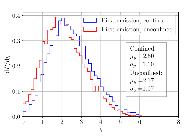
Given a specific parameter set, table 1, the probability distribution in rapidity for the first emission, , is shown in figure 2. This distribution has a mean at around two units of rapidity. Thus, on average, a new emission is assigned a rapidity of roughly two units larger than the mother (or emitter) dipole. It is worth noting that the inclusion of confinement effects slightly increases the mean as compared to the unconfined distribution. This is caused by the additional suppression of large dipoles, requiring large dipoles to be discarded in the evolution and an emission at a larger rapidity to be tried.
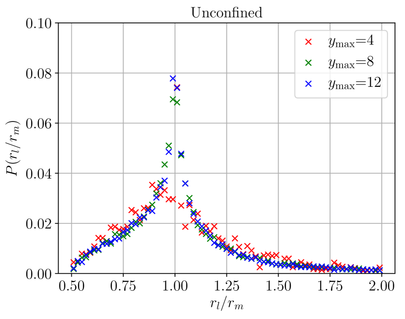
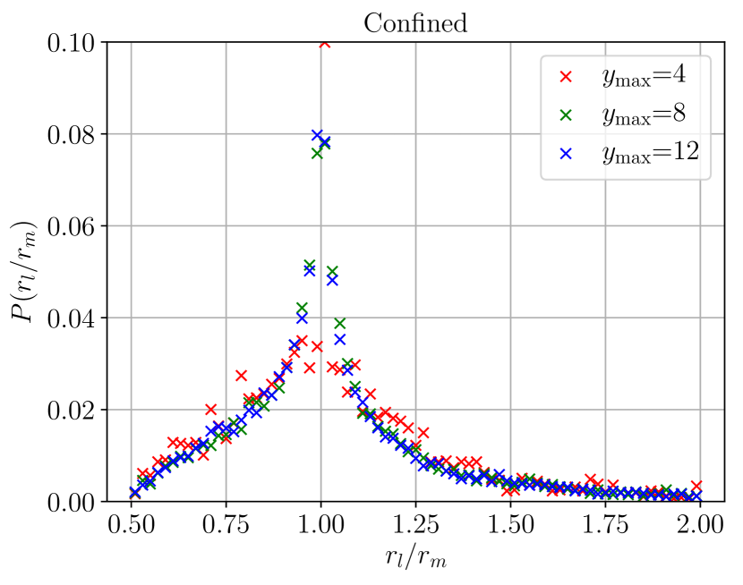
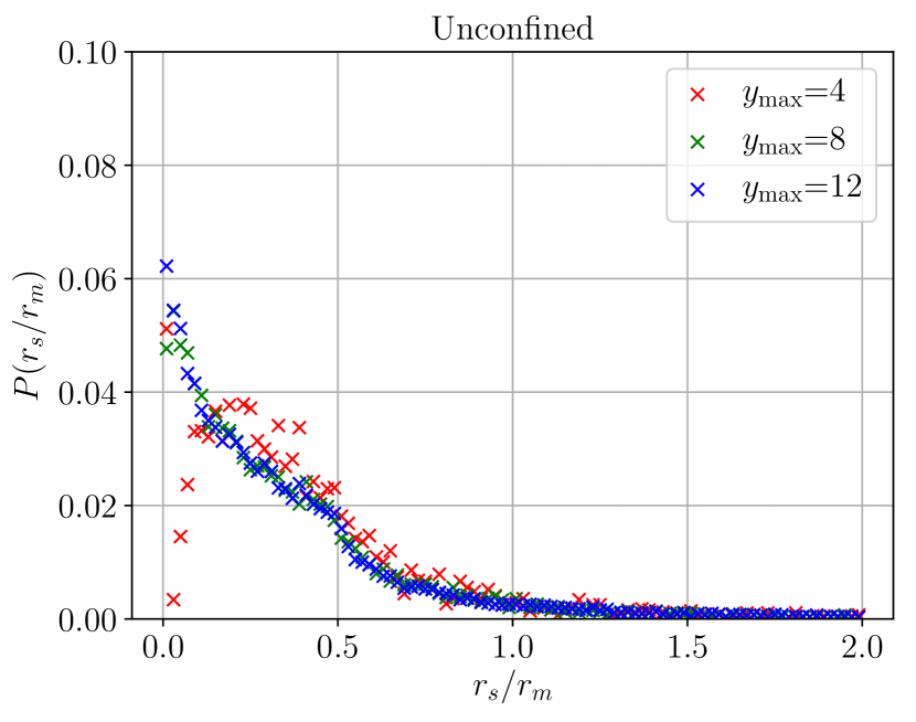
In each step of the dipole evolution a mother dipole is split into two daughters. Figure 3 shows the distribution in sizes of the smaller and larger dipole, scaled w.r.t. their mothers’ size for three different evolutions (). Here, it is evident that on average the larger dipole retains the size of the mother, while the distribution of the smaller is much broader. At lower there is a bump in the distribution at around 30-40% of the mothers size, while this bump is less pronounced at larger maximal rapidity.
(a)
(b)
(c)

(d)
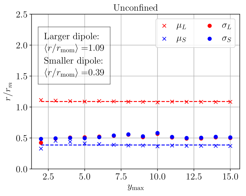
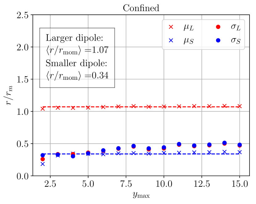
Figure 4 shows the corresponding average and standard deviation in the lengths of all the daughter dipoles scaled w.r.t. the length of their mothers’, as a function of maximal rapidity of the evolution. As stated above, it is clear that while the larger of the two daughter dipoles can be taken to be identical to the mother dipole, the size of the smaller dipole has larger fluctuations. The average size of the smaller dipole is, however, fixed at roughly a third of the mother dipole for all .
(a)
(b)
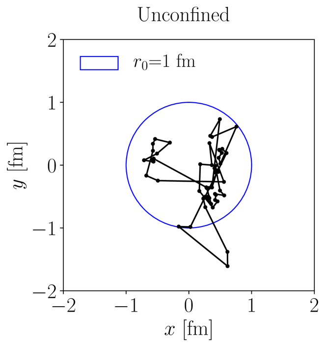
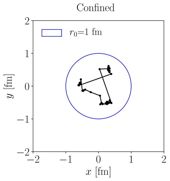
After a full evolution, an initial proton consisting of three dipoles will have evolved to a larger set of dipoles of mostly smaller sizes than the initial dipoles, cf. figure 5. From these two figures it is evident that the effect of confinement plays a large role in the evolution, effectively reducing the number of large dipoles in the final configuration. Thus, as , confinement is expected to play a large role when evaluating the cross sections. Confinement also introduces more activity – or hot spots – around the endpoints of the dipoles.
(a)
(b)
4.4 Pascal approximation for dipole evolution
The full dipole evolution can be approximated based on the geometric observation above. On average one dipole splitting happens per two units of rapidity, and the lengths of the two resulting dipoles after the splitting, are approximately equal to and one third the size of the mother dipole respectively. This behaviour is tabulated in table 2 for four generations of evolution. Similar results have been observed within the Dipsy framework, although their dipole swing slightly increases the size of the smaller dipole in a branching Avsar:2007ht to half of the size of the mother dipole.
| y = 0 | y = 2 | y = 4 | y = 6 | y = 8 | |
|---|---|---|---|---|---|
| 1 | 1 | 1 | 1 | 1 | |
| 0 | 1 | 2 | 3 | 4 | |
| 0 | 0 | 1 | 3 | 6 | |
| 0 | 0 | 0 | 1 | 4 | |
| 0 | 0 | 0 | 0 | 1 | |
| 1 | 2 | 4 | 8 | 16 |
The number of dipoles in table 2 follows the coefficients of the binomial theorem, with the number in column row being equal to , and can thus be arranged to form Pascal’s triangle. The total number of dipoles after a given number of generation, as well as the number of dipoles of a certain size, can be quickly approximated this way. Knowing the positions of the initial dipoles and the emitted dipole sizes, positions of all dipoles can also be inferred.
To exploit further these simple relations in the dipole evolution, we have created an alternative toy-model denoted the Pascal approximation. Here, the step size in rapidity () and the size of the smaller dipole () in a branching are implemented as tunable parameters, with the size of the mother dipole and a tunable fraction. The number of steps taken in total is calculated from the step size, with and given in eqs. (25–26). To mimic the recoil effects in the full dipole evolution, a Gaussian smearing of the daughter lengths is introduced with mean for the larger and smaller daughters, respectively. Knowing the lengths of the mother and daughter dipoles, they are placed in transverse space by calculating the angles of the triangle spanned by the endpoints of the three (connected) dipoles.
This simple approximation is useful for introducing toy-models for sub-leading effects, such as confinement and saturation, as basic quantities like total number of dipoles after a given evolution, can be calculated analytically. A crude model for confinement is introduced by requiring the length of the emitted dipoles to not exceed a tunable maximally allowed cutoff, . If this occurs, the branching is discarded and the next step in rapidity is tried. Once the full evolution has occurred, each of the dipoles are allowed to interact using the dipole-dipole scattering amplitude given in eq. (2.2) (or eq. (28) for the confined version).
(a)
(b)
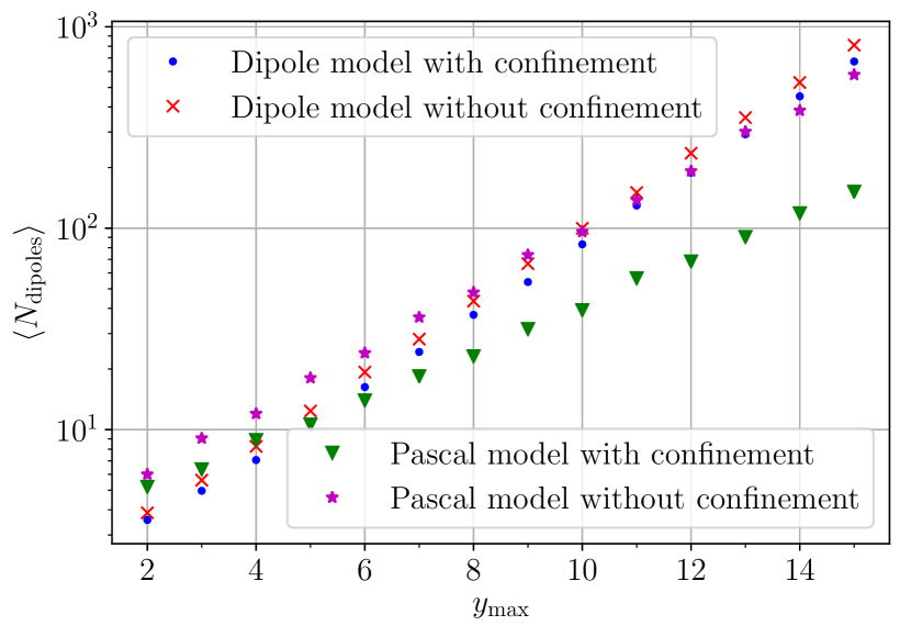
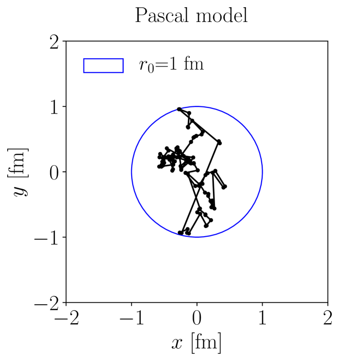
In fig 6(a) the average number of dipoles in a single proton after a full evolution to maximal rapidity is shown. The same parameters as given in table 1 are used, while the parameters are extracted from figures 2 and 3. The unconfined Pascal model follow the same trend as the full dipole model, albeit having a slightly larger average number of dipoles at small maximal rapidity. It is evident that the confined Pascal model has a different slope than the full dipole model and the unconfined Pascal model, with the effect of the crude model for confinement clearly seen at large . Here, the confined Pascal model results in a smaller average number of dipoles as compared to the full dipole model.
In figure 6 (b) the dipole configuration of an evolved proton for is shown. This has more features in common with full, unconfined dipole evolution than full, confined dipole evolution, with dipoles being more randomly distributed, than focused around hot spots.
A practical advantage of the Pascal approximation, besides being a toy model for testing models for sub-leading effects, is its computational speed. For simple cascade-quantities like numbers of dipoles, results can be calculated analytically. With inclusion of geometry, event-by-event results can be generated approximately a factor of 1000 faster, for large maximal rapidity (). It thus serves as a decent replacement for the full dipole evolution model for calculation of cascade properties with limited computational resources. For full calculations of amplitudes and cross sections, the efficiency gain is not nearly as large, as in that case the bottleneck is the calculation of all in eq. (2.2).
4.5 Dipole-dipole interactions
The dipole-dipole interactions are defined to occur at rapidity zero and given by eq. (2.2). If confinement is introduced in the splitting kernel (eq. (27)), one also has to change the interaction probability in order to make the event generation consistent. This modifies eq. (2.2) to
| (28) |
where is the modified Bessel function and the maximally allowed size for a dipole in the evolution.
The choice of collision frame, however, is not trivial. Obviously, no observables should depend on the frame-choice of the collision. In practice, the choice does matter, as no sub-leading color corrections are included in the dipole evolution. Previous studies have shown that for symmetric systems, e.g. collisions, the optimal frame choice is the center-of-mass (CM) frame Mueller:1996te . This is also utilized in our approach, cf. eq. (25), where both beams are evolved the same distance in rapidity. In asymmetric systems, such as or systems, the CM frame lies more towards the heavier of the two objects, and it has been previously argued that the optimal frame here would be the rest frame of the heavier beams Mueller:1996te . This, however, is not the choice we have taken. The maximal rapidity chosen in eq. (26) is found in what we call the center-of-rapidity frame. Here, both beams are evolved the same distance in rapidity, similarly to what is chosen in symmetric collision systems. As already stated, this work does not attempt to include sub-leading colour effects in the evolution, thus frame-independence is not possible to obtain. Hence the simplest choice has been made to use the same frame for all systems, i.e. the center-of-rapidity frame given in eqs. (25–26).
4.6 Assigning spatial vertices to MPIs
In order to utilize the formalism developed so far in real , and events, the dipole cascade is matched to the Pythia 8 MPI model Sjostrand:1987su . This allows for evaluation of geometric initial state quantities, such as eccentricities (see section 3.2), at fixed number of charged hadrons in the final state, using a similar definition of charged particles as the experiments. The Pythia 8 MPI model considers collisions, treating all partonic sub-collisions as separate QCD scatterings, which are uncorrelated up to momentum conservation. Other factors present in the MPI model is a rescaling of the parton density between each scattering, preservation of valence quark content and a sophisticated treatment of beam remnants Sjostrand:2004pf .
In the MPI framework, the sub-collisions and their kinematics are selected using the normal QCD cross section. But since this cross section diverges at low , the expression is regulated using a parameter, :
| (29) |
For matching of vertices to each individual partonic sub-collision, it is also useful to note that MPIs are generated in decreasing order of , starting from a (process-dependent) maximal scale. This decreasing order is generated from a Sudakov-like expression of the form:
| (30) |
with given by eq. (29). The impact-parameter of the collision is also taken into account in the evolution by connecting the average number of MPIs to the overlap of the two colliding protons. This introduces additional factors of in eq. (30) along with the need to select the impact parameter consistently.444Here , where is constrained by the ratio of the dampened QCD cross section in equation (29) to the total non-diffractive cross section. Furthermore, new partons are generated by initial- and final-state radiation.
Recently, a method of assigning space-time information to the MPIs in Pythia 8 was introduced Bierlich:2017vhg . Here, the transverse coordinates are sampled from a two-dimensional Gaussian distribution defined by the overlap of the mass distributions of the two colliding protons. The width of the Gaussian is a free parameter (which should not be too far from the proton radius) and a mean equal to the impact parameter chosen in the MPI framework. Initial- and final-state radiation are then treated as small displacements of the selected anchor points of the MPIs. This introduces and additional smearing of an MPI vertex whenever a parton is radiated off from the partons involved in the MPI. The smearing is done using another Gaussian with a width of , where is a parameter with default value GeVfm.
In this work, we utilize the dipole framework to generate the space-time vertices, instead of the default two-dimensional Gaussian distribution. We currently do not use the dipole model to generate the -spectrum for the MPIs, but retain the -distribution obtained internally with Pythia 8. This means that the dipole model is only used to obtain information on the spatial location of the MPIs. Using the dipole framework to generate space-time vertices requires (as with the Gaussian model) some assumptions, as this matching can not be derived from first principles. In order to obtain a reasonable matching, the following is noted:
-
•
Each branch of the (projectile) dipole cascade can be identified as a virtual emission, which goes on shell if, and only if, it collides with a corresponding virtual emission from the target.
-
•
Each proton–proton collision has many potential sub-collisions between all combinations of virtual emissions. We order the sub-collisions in terms of contribution to total cross section, thus the MPI with largest is identified with the dipole-dipole scattering with the largest .
The concrete matching is done by first generating two dipole cascades, and allowing them to collide with the same impact parameter used in the generation of the MPIs. This produces a list of possible dipole–dipole collisions, each with an interaction strength . As the MPIs are generated (from hardest to softest), they are each assigned a vertex sampled from this list with a weight equal to , normalised to the summed dipole-dipole interaction strength (and not the unitarized interaction). The vertex is simply given as the mean of the transverse coordinates of the dipoles in the interaction. Once a set of dipoles have been assigned to an MPI, they are both flagged as used, and cannot initially be re-used to ensure a reasonable spread. In cases where the list runs out of interactions containing only unused dipoles, the dipoles are allowed to re-interact, though not with the same dipole as initially.
As opposed to the default model, vertices are now selected from a distribution which event-by-event is asymmetric, and contains ”hot spots” with large activity, as shown in figure 5 (b) for the full evolution including confinement effects.
The matching of largest to hardest MPI requires further discussion, as one could argue the opposite. The dipole-dipole scattering amplitude is driven by the distances between the endpoints of the interacting dipoles, as indicated in figure 1. One can argue that small corresponds to small distances, which in turn corresponds to large of the gluons emitted in the interaction. Hard MPIs would with this reasoning correspond to small . This is indeed the choice made in the Dipsy event generator for exclusive final states Flensburg:2011kk , but opposite to the choice made above. We do, however, also note that the exclusive final states generated by Dipsy describes spectra of charged particles poorly, in particular the high- part of the distributions vastly overshoots data. We therefore currently refrain from associating the dipole sizes directly to the of emerging partons, but rather give larger attention to the cross section. We note that large interactions dominate the cross sections. A guiding principle is therefore to ensure that such interactions are always identified with an MPI, by assigning it first.
There are several possible future improvements of the matching technique. A small improvement of the existing technique, could include to also identify initial state radiation with emissions going on shell, and assign them vertices from the cascade as such. Going beyond improvement of matching techniques, would be a full re-evaluation of the MPI model, with the dipole cascade and interactions as a starting point. The consequences of such an approach could be studied in a toy-model where the obtained with the dipole formulation could be utilized instead of the ’s obtained within the Pythia 8 model. It would then be possible to study if this method gives rise to similar problems as the Dipsy MPI description has in the high tail.
Instead of creating a completely new model like Dipsy, it should be possible to use the dipole model to improve the existing Pythia 8 model. A first step would be to replace in eq. (30) with a dynamically calculated cross section, event-by-event. Secondly, the parameter in eq. (29) could be re-evaluated in terms of the dipole model. The physical interpretation of in the MPI model, is that of a colour screening scale. The perturbative treatment of eq. (30) would naively break down at some minimal scale , where is the (colour screening) size of a proton, left as a free parameter. In the dipole model, this colour screening length could be identified as either the transverse size of the cascade after the evolution, or the length of the largest colour connected dipole chain. In that way the energy dependence of would also come for free, instead of having to assume a power-law dependence, as is the default assumption in Pythia 8.
4.6.1 Heavy ion collisions
The method described above can be directly applied to heavy ion collisions as they are modelled in the Angantyr framework for heavy ion collisions in Pythia 8 (see appendix B for a brief review, and refs. Bierlich:2016smv ; Bierlich:2018xfw for a full description). In the Angantyr model, sub-collisions are chosen using a Glauber-like approach. Sub-collisions are in turn associated with one out of several types of pp events, depending on the properties of the sub-collision. Since all these events are generated using the MPI model described above, the generalization is only a matter of generating vertices for each sub-collision in its local coordinate system, and then moving them to the global coordinate system defined by the Glauber calculation.
5 Results I – comparing cross sections
In this section we present results on integrated cross sections for and collisions. For we present results for both the dipole evolution model and for the Pascal model, while for we focus our attention on the dipole model. The main purpose of this section is tuning: the model parameters have to be estimated by comparisons with data, preferably data that we do not aim to make predictions for in later sections.
It is thus not the aim of this section to be able to describe the cross sections perfectly – but more generally, to get an overall agreement between model and data, especially at LHC energies, where we aim to make predictions for the substructure observables.
More dedicated models are available to describe the cross sections at all energies, from the GeV range to the TeV range, results of which are shown alongside results from the dipole model in the section. The most widespread model is based on the 1992 total cross section fit by Donnachie and Landshoff (DL) Donnachie:1992ny and the models for elastic and diffractive cross sections by Schuler and Sjöstrand (SaS) Schuler:1993wr . Another, more recent model by Appleby et al. (ABMST) Appleby:2016ask is more complex than SaS, and able to describe latest LHC data better. The models are both implemented in Pythia 8, with some additions to the original models Rasmussen:2018dgo . In this paper we compare to the original models, and not those adapted to Pythia 8.
5.1 Results for
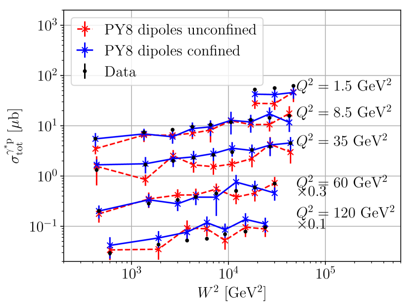
We begin with the results on photon-proton total cross sections. Here, we compare the dipole evolution model to data obtained from H1 Adloff:2000qk at different energies and virtualities. We note that the photon wave function implemented only includes the three lightest quarks, and none of the vector meson states present at low . Thus we expect the results to be less precise at low virtualities, where the probability for the photon to fluctuate into a hadronic state becomes non-negligible. Similarly, the masses of the quarks should be taken into account if the argument of the Bessel functions become close to the squared quark masses, i.e. if
| (31) |
occurring in the limits or if small. The contribution from -quarks are neglected for simplicity, the uncertainty arising from this approximation is discussed at the end of the section.
The H1 data presents results on the proton structure function at a large range of virtualities and energies. This is translated into a photon-proton total cross section as follows:
| (32) |
with the CM energy given as and a unit conversion factor.
(a)
(b)
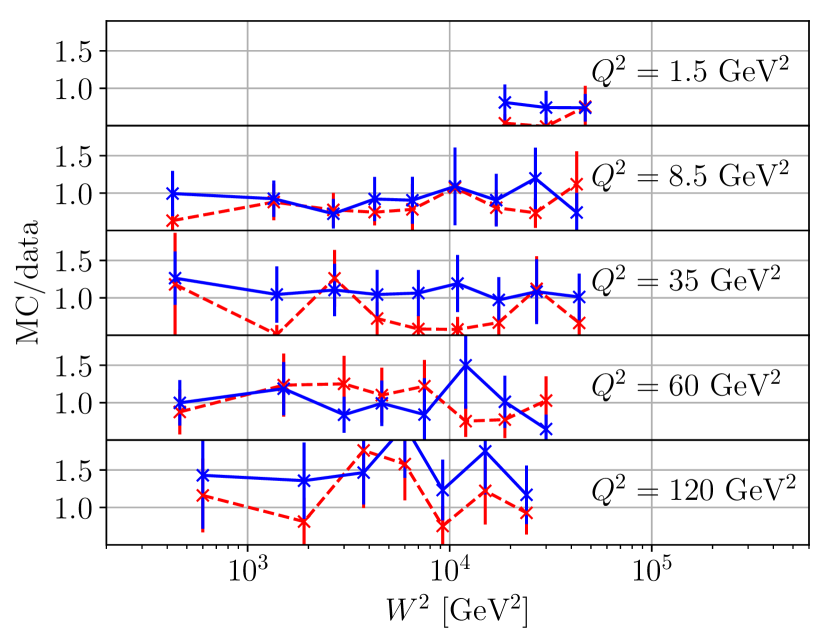
It is evident from figure 7 that we undershoot data at low . At intermediate virtualities the model does a fairly good job, while at the highest virtuality probed the prediction overshoots data with roughly 50%. In order to quantify the performance of the models, a test has been performed, taking into account the errors of the measurement:
| (33) |
with denoting the cross section measured in data at a given squared energy , the model prediction for that squared energy and the variance of the data and model predictions, respectively.
The model has been tuned with the Professor2 framework Buckley:2009bj , and the parameters are shown along with the in table 3. The parameters of the tune are reasonable, giving a initial dipole size roughly of order 1 fm with a width of the Gaussian fluctuations at around fm. Adding confinement allows for a slightly larger initial dipole size, as the largest dipoles in the evolution will be suppressed as compared to the unconfined model, while also the upper integration limit on the photon is allowed to increase when turning on confinement. The width of the fluctuations and the strong coupling appear not to be affected by the confinement effect. Taking the full H1 data set into account, the confined model gives a reasonable , and performs slightly better than the unconfined model.
| Parameter | unconfined | confined |
|---|---|---|
| [fm] | 1.08 | 1.15 |
| [fm] | - | 3.50 |
| [fm] | 0.10 | 0.10 |
| [fm] | 2.07 | 2.56 |
| 0.21 | 0.22 | |
| (shown values) | 2.41 | 0.57 |
| (full H1 data set) | 2.99 | 1.98 |
Since the charm contribution to the cross section has been neglected, an assessment of the uncertainty arising from this approximation should be made. Adding massless charm quarks shifts the total cross section upwards by 67%, estimated by the ratio:
| (34) |
This rise in cross section can be tuned away in a way similar to the procedure described above. Adding quark masses (lighter quark masses neglected) reduces the contribution. The reduction is larger for smaller . The quantitative effect of adding masses was studied in ref. Avsar:2007ht . For small the decrease compared to the massless charm case is and for large the decrease is . Both represent un-tuned values. A conservative, un-tuned estimate of the uncertainty in figure 7 from neglecting (massive) charm quarks is therefore up to . Retuning will allow for shifting the cross section upwards in the low region where the values in figure 7 undershoots, improving the overall agreement.
5.2 Results for
In figure 8 we show the total cross section as a function of CM collision energy for both the full dipole model (a) and the Pascal model (b). Both figures show results using the confined (solid blue lines) and unconfined (dashed red lines) models as well as the ABMST (solid green lines) and SaS+DL model (solid magenta lines). It is evident that the full dipole model undershoots data at low , whereas it agrees with data at roughly GeV, with the confined model having a smaller (cf. table 4) than the unconfined model using only this data set. The Pascal model, figure 8 (b), shows an overall shift towards higher cross sections as compared to the full dipole model, thus describing the lower energies well while slightly overshooting the higher energies. With only this data set, both Pascal models have a lower than the dipole models. As explained in section 4.4, the key difference between the models, is the treatment of confinement as a hard cutoff. In both figures, it is evident that both the SaS+DL and ABMST models perform better, not surprising as these models have been created to reproduce (a subset of) this data.
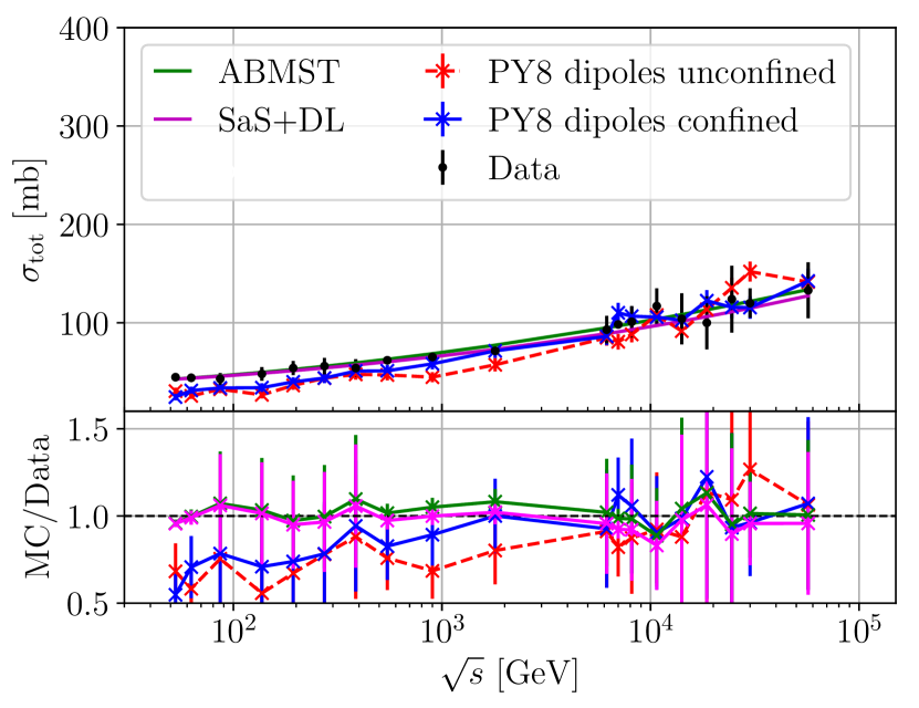
(a)
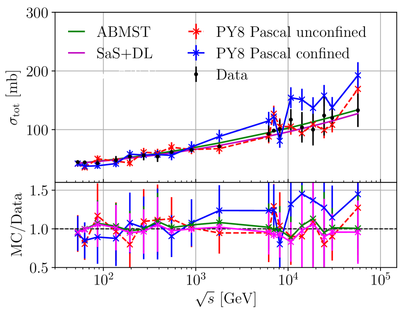
(b)
In figure 9 we show the elastic cross section for the full dipole model (a) and the Pascal model (b). Neither of the dipole models are able to describe this cross section, being roughly 50% below data in the entire energy range, except for the very last bins, i.e. at LHC energies. The Pascal model, however, agrees with data at lower energies better than the full model. Also here, the two dedicated models describe the elastic data better than the dipole and Pascal models, with the SaS+DL model deviating from the data at LHC energies, while ABMST describes data in the entire energy range. This is partly due to a modification of the elastic slope in the SaS model, and partly due to the additional trajectories included in the ABMST model: where SaS+DL only contains a single Pomeron in the description of the elastic cross section, ABMST has two – along with additional terms not dominating at these energies. This of course introduces more freedom to the model, thus a better agreement with data at high energies.
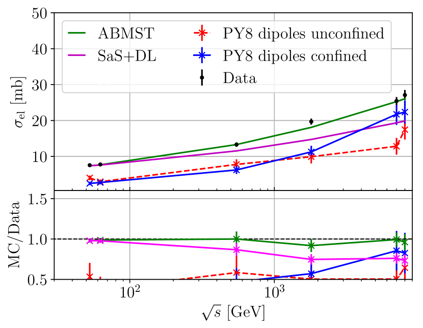
(a)
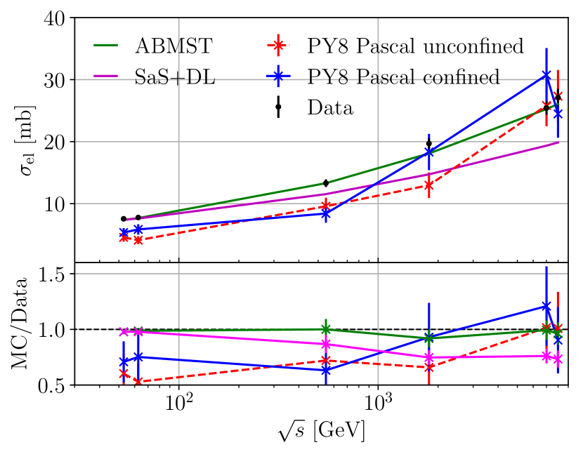
(b)
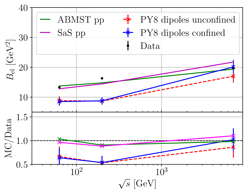
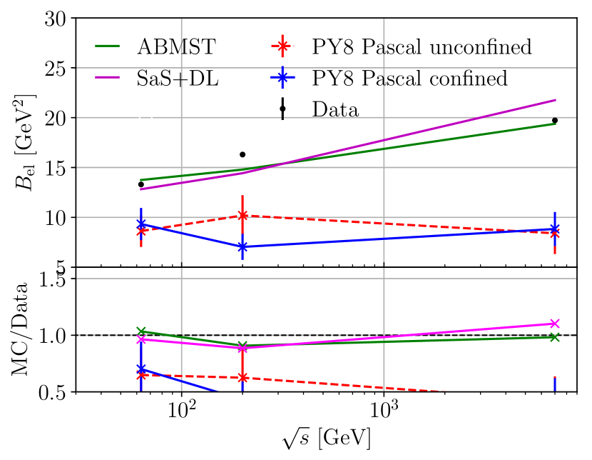
The last result is the elastic slope at , shown in figure 10. Second to the total cross section, this is the most important distribution for us to describe, as this is sensitive to the internal structure of the proton, i.e. the actual impact parameter value used in the calculation, while e.g. the elastic cross section is only sensitive to the average impact parameter. Figure 10 again shows the results for the full dipole model (a) and the Pascal model (b). Here, both models are undershooting the data by roughly 50% in the entire energy range, except that the dipole model is able to describe data in the very last bin. Also here, the ABMST and SaS+DL models predictions are closer to the data than the dipole and Pascal models.
We expect that the introduction of a running strong coupling will aid in the description of the data. This introduction appears in two places: in the dipole evolution and in the dipole-dipole scattering. A larger strong coupling in the evolution decreases the average step size in rapidity and increases the average size of the emitted dipoles, thus allowing for a larger number of larger dipoles at the end of the evolution. This, along with the increased dipole-dipole scattering cross section with increased strong coupling, would essentially increase all the cross sections, and thus also the elastic slope. The scale choice in such a running coupling would not be obvious, however, and we thus postpone the inclusion of a running coupling to future work.
(a)
(b)
The combined results on , and the elastic slope deserves a further comment. From the optical theorem the differential elastic cross section is:
| (35) |
Neglecting the real part of the amplitude puts . The left hand side is often approximated by an exponential: , giving when integrated over . The results in figures 8, 9 and 10 are not in agreement with this simple proposition. This can either mean that the exponential approximation is not a good one (which is manifestly true for large ), or that the shape of in our model simply is too narrow, such that the elastic cross section and hence is not well described. If the latter is the case, a solution to the problem could be to include more dipoles than three in the initial proton state. This would increase the total and elastic cross sections at low , while the effect at higher could be tuned away by a slightly smaller value of or . Other studies of proton substructure Albacete:2017ajt has indicated that the number of hot-spots required for a satisfactory qualitative description of LHC data is larger than three, but at the same time, previous studies of the Mueller dipole formalism in the DIPSY event generator Avsar:2006jy indicated that a triangle configuration of initial dipoles is the most suitable choice for a good description of the cross sections. A study of this sort will therefore likely have to rely on attemps of simultaneous description of both sub-structure and cross sections, and will be referred to a future study.
Table 4 shows the parameters obtained when tuning to all three observables () using Professor2. We also show the for three data sets of various sizes. It is striking that the inclusion of the elastic cross section to the -calculation swaps the behaviour of the full dipole model – without the elastic data set, the confined model has a lower than the unconfined model, while the opposite is true with the inclusion of the elastic cross section. This swap is caused by the first two data points in the elastic cross section, where the unconfined version of the full dipole describes data slightly better than the confined version. The parameters of the dipole model obtained with the tunes show the behaviour also observed in : adding confinement allows for an increased initial dipole size and slightly larger fluctuations around this size. The initial dipole size seems reasonable for both the confined dipole model and the unconfined Pascal model, giving sizes of the order fm also confirmed by Dipsy ( fm) and proton charge radii measurements (giving roughly fm).
| Full dipole model | Pascal model | ABMST | SaS+DL | |||
| Parameter | unconfined | confined | unconfined | confined | ||
| [fm] | 0.53 | 0.70 | 1.20 | 1.10 | ||
| [fm] | - | 3.00 | - | 2.05 | ||
| [fm] | 0.17 | 0.27 | 0.10 | 0.10 | ||
| 0.24 | 0.22 | 0.15 | 0.16 | |||
| - | - | 0.25 | 0.40 | |||
| - | - | 2.20 | 2.45 | |||
| : | 5.22 | 3.34 | 0.75 | 1.04 | 0.28 | 0.41 |
| : , | 6.89 | 5.40 | 2.80 | 5.34 | 0.25 | 0.34 |
| : , , | 11.21 | 13.67 | 4.63 | 5.14 | 0.20 | 0.46 |
As already stated, the inclusion of a running strong coupling is expected to improve results for both the dipole and Pascal model. As we currently are aiming to describe proton substructure at the TeV scale, we can, however, ignore the small deviations from and at lower energies for the moment.
6 Results II – eccentricities in small and large systems
In this section we turn our attention to predictions related to the geometry of an event. The parton-level eccentricities of both small and large systems are examined using the matching between the dipole model and the MPI framework described as in section 4.6. Results from the dipole model555We do not show eccentricities calculated using the Pascal approximation, as it is, at this point, mainly intended as a toy model. If the Pascal approximation should be used for studies of eccentricities, we should point out that the large spread in daughter sizes as seen in figure 4 must be incorporated, in order to provide reasonable estimates for flow fluctuations. are shown along with the default models of Pythia 8: in collisions, the default scheme of Pythia 8 is a transverse placement according to a 2D Gaussian, while for larger systems two default Pythia 8 methods are available – the usual Glauber approach and the 2D Gaussian model extended to larger systems. In order to compare to data, all events are hadronized with Pythia 8 after the parton-level eccentricities are calculated. Results are presented and in a single case compared to data from ALICE Acharya:2019vdf . Parton level eccentricities were calculated with a weighting, cf. section 3.2, and events accepted if they passed the ALICE high-multiplicity trigger. Eccentricities and normalized symmetric cumulants are presented as a function of average central multiplicity ().
Recall from section 4.6 that Pythia 8 includes a -dependent Gaussian smearing of parton vertices in the initial- and final-state shower. It is not clear from first principles whether such effects should be included in the calculation of geometric quantities or not. Consider, on one hand, creation of a QGP at early times, right after the collision. Here a parton shower will not be able to influence the geometry of the event, before a hydrodynamic response should be taken into account. On the other hand, one can imagine a system with large gradients (such as a small collision system) which will take time to hydrodynamize, and will therefore be influenced by geometric fluctuations from the final state shower as well. It is important to note, however, that no QGP is assumed in any results presented below as no QGP is assumed in neither Pythia 8 nor Angantyr.
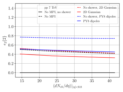
Opening up for a discussion, we show results in figure 11 with and without shower. It is evident that the eccentricities are vastly affected by the models. First consider the simplest case, i.e. placing all MPIs in the proton center and not introducing any shower smearing. This gives no eccentricity as expected, cf. solid black line in figure 11. Symmetric distributions, such as the 2D Gaussian shower smearing and the MPI vertex assignment, should in principle give no eccentricity. But, as we are sampling only a finite number of MPIs from such symmetric distributions, an eccentricity does appear for these models, cf. dashed red and dashed black lines of figure 11. The two methods overlap, thus the exact same effect can be introduced with either (a) no MPI vertex assignment with a Gaussian smearing from the shower or (b) a Gaussian MPI vertex assignment and no shower smearing. That the two overlap is not so surprising as both are Gaussian smearings, and applying such a smearing during the shower or assigning it to the MPIs should make no difference: both methods give rise to a more lenticular overlap region of the two colliding protons.
Applying Gaussian smearing twice, i.e. both in the MPI vertex assignment and during the shower smears the lenticular shape from the MPI assignment slightly, thus causing the eccentricity to drop, cf. the solid red line in figure 11. The largest effect on the eccentricity is seen when purely considering MPI vertex assignment with the dipole model, cf. the dashed blue line in figure 11. The eccentricity with the dipole model is approximately twice as large as with the Gaussian model, thus indicating that event-by-event asymmetries in the initial state gives rise to larger fluctuations and thus larger eccentricities. Adding the Gaussian shower smearing on top of the dipole model, solid blue line of figure 11, washes out some of these features – i.e. makes the almond shape of the overlap region rounder.
(a)
(b)
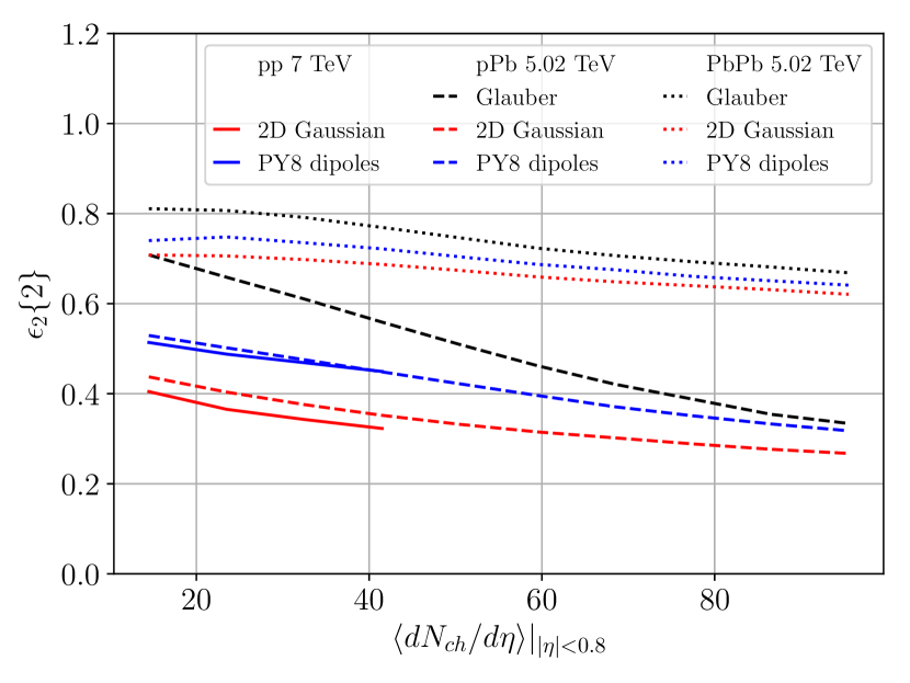
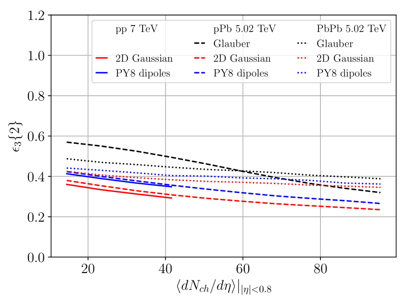
Figure 12 shows the eccentricities in three different systems. Beginning with we observe in that the dipole evolution gives rise to a larger eccentricity than the 2D-Gaussian. In the dipole evolution, the asymmetry is built in at the cascade level, where in the 2D-Gaussian, where MPIs are sampled from a symmetric distribution, asymmetry only arises due to the sample size. Proceeding to larger systems, and , it is evident that the same trend is seen: the dipole model gives rise to larger than the symmetric model. The Glauber model, however, is consistently larger than the other two models at low multiplicity, while all three models appear to approach the same eccentricity at higher multiplicities. Thus it becomes evident that the proton initial state does have an effect on eccentricities, and that it is especially evident in low-multiplicity events, e.g. peripheral collisions.
Unfortunately, the low-multiplicity events are often marred by large non-flow effects. Measuring the eccentricities with higher-order cumulants can remove some of the contributions from non-flow, thus making it easier to compare data to models. We present results for with higher-order cumulants in appendix C, as the results are similar in shape as figure 12, but differ in normalisation. Figure 12 (b) show for all three systems. Here, it becomes more difficult to distinguish between the models in symmetric systems, while a large discrepancy between the Glauber approach and the other two is seen in .
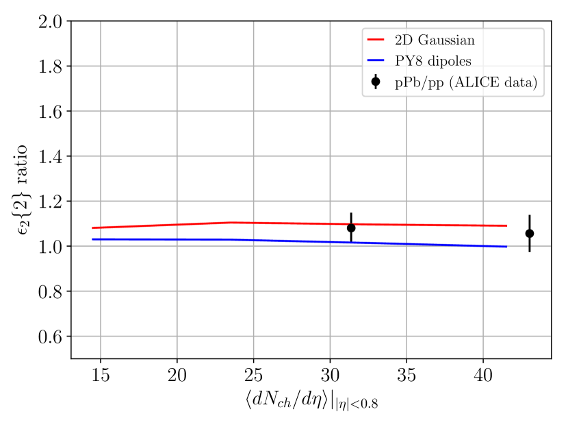
Another feature seen in figure 12 is that the dipole model gives roughly the same results for in both and collisions. If one assumes that the response functions are the same for the two systems (however one may have obtained these response functions, QGP or by string-string interactions), the ratio of to eccentricities should thus be comparable to the ratio of flow coefficients measured with the ALICE detector. This ratio is shown in figure 13 for the second-order eccentricity. Both the Gaussian and dipole models are compatible with the ALICE data, however, so we cannot presently discriminate between the two. Additional measurements of the flow coefficients in low-multiplicity events are thus required in order to discriminate between models in this observable.
(a)
(b)
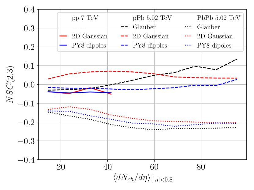
Figure 13 (b) shows the normalized symmetric cumulant, . This has been constructed to study the correlations between the eccentricities and normalized to the uncorrelated eccentricities in order to remove the effects of the response function. ALICE reports that all three systems have the same at the same average multiplicity, indicating that the correlation between the flow coefficients are the same in different collision systems. We observe no such effect. Focusing on the dipole model, the correlations appear equal in magnitude for and , but results are consistently below the smaller systems. Results for the Gaussian model shows no similarities at all between systems, as the is positive, while and are negative. Thus the normalized symmetric cumulants for systems would be an ideal place to discriminate between the symmetric and asymmetric initial state. results for all three models are in agreement with IP-Glasma predictions presented in the ALICE paper. The main difference between the dipole model and the IP-Glasma approach is the inclusion of saturation in the cascade of the latter. As the two approaches give similar results, we do not find that saturation plays a large role in this observable.
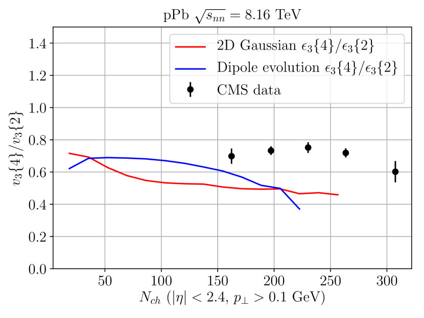
6.1 Flow fluctuations in pPb collisions
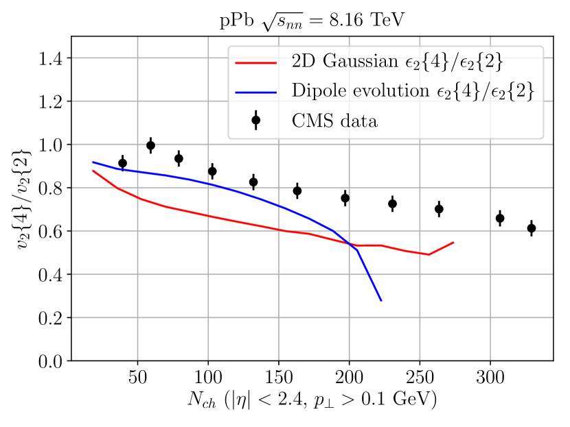
Recently, CMS presented results on multi-particle correlations using higher-order particle cumulants in collisions Sirunyan:2019pbr . Ratios of the flow-coefficients based on these cumulants were presented, including the first measurements of the ratio of in . In figure 14 we show the predictions for the ratios with the confined dipole model and the default Gaussian model as a function of multiplicity. Both models reasonably reproduce the shape seen in the elliptical ratio, figure 14 (a) showing , while the normalisation of the dipole model is slightly better than with the Gaussian model. For the triangular ratio, figure 14 (b), both models appear to undershoot data at high multiplicities, where data is available. As opposed to model predictions presented in the CMS paper Giacalone:2017uqx ; Bernhard:2016tnd , our predictions have not been applied a 10% ad hoc increase in normalisation. And where the model predictions presented in Giacalone:2017uqx ; Bernhard:2016tnd predicts roughly the same ratio for both and , neither the dipole nor the Gaussian model predicts the same normalisation for the two ratios, cf. the height of figure 14 (a) and (b) differs.
(a)
(b)
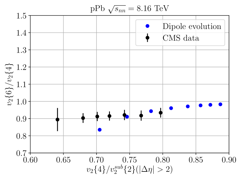
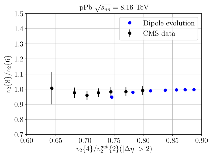
Figure 15 shows the higher-order cumulant ratios for elliptic flow as a function of the lower-order ratio presented in figure 14 (a). For higher order cumulants, the Gaussian model predicts purely imaginary values for even powers of the cumulants, hence it has been left out of the figures. The dipole model, however, is able to describe data reasonably well. The dipole predictions decrease with decreasing ratio in figure 15 (a), while being roughly constant at unity in figure 15 (b). This is in accordance with the model predictions presented by CMS Yan:2013laa , assuming a non-Gaussian model for the initial state. We note that the eccentricities presented with the dipole model here are (a) based on a pQCD model, and (b) related to final state multiplicities calculated in the same acceptance as the experiment.
(a)
(b)
7 Results III – dynamic colour fluctuations in Glauber calculations
A general feature of several models describing both collisions of protons and of nuclei, is the notion of interacting nucleons and nuclear sub-collisions, calculated in the formalism of Glauber Glauber:1955qq ; Miller:2007ri . The basic formalism is mainly concerned with calculating the full scattering matrix or amplitude from knowledge of the nucleon-nucleon amplitude and spatial positions. Multiple interactions between nucleons factorize in transverse coordinates, so in the eikonal limit the -matrix for scattering between two nuclei and becomes:
| (36) |
where and denote the individual nucleons, is the nucleus–nucleus impact parameter and is the nucleon–nucleon impact parameter. We will here consider the simplifying case where only one projectile (either p or , called below) collides with a nucleus (A), which reduces eq. (36) considerably:
| (37) |
If no fluctuations in the interaction are included, the projectile-nucleon elastic amplitude can be inserted, and the total and elastic cross sections can be calculated directly from eqs. (11–12). If fluctuations for projectile and target are included, as calculated for example in the dipole model, the amplitude will depend on the states of target () and projectile () respectively. As shown in section 3.1, the elastic amplitude can be calculated as an average over all states. In ref. Alvioli:2013vk it was pointed out that in the evaluation of such an average, the projectile must remain frozen in the same state throughout the passage of the target. Similar to eq. (3.1) the elastic profile function (at fixed Mandelstam ) for a fixed state () of the projectile scattered on a single target nucleon (all states) becomes:
| (38) |
where previously suppressed indices and on are spelled out for clarity. For a projectile-nucleus collision, with the projectile frozen in the state , the relevant projectile-nucleon () amplitude becomes:
| (39) |
In the short hand notation on the right hand side, the average over the repeated index is suppressed. This is the amplitude used to determine which nucleons are “wounded” in a collision. If the purpose is to determine which nucleons participate in the collision either elastically or inelastically, the differential wounded cross section can be calculated with the normal differential pp total cross section as an ansatz, from eq. (11). Since the projectile should be frozen in the state , the expression for from eq. (39) is inserted to the differential total cross section. This just recovers the normal total projectile-nucleon cross section:
| (40) |
In a Monte Carlo, the number of wounded nucleons can then be generated by assigning each projectile or nucleon a radius of , where the expression in eq. (40) has been integrated over to give . Normally one is not interested in the number of wounded nucleons including elastic interaction, but rather those that contribute to particle production (i.e. where there is a colour exchange). A usual approach is to just use the inelastic cross section in place of in the Monte Carlo recipe. This does, however, not account fully for colour fluctuations, as the inelatic cross section is modified when averaging over target states with a frozen projectile. Instead of directly using the inelastic cross section in the Monte Carlo, the modified cross section should be used. This cross section was dubbed the “wounded cross section” in ref. Bierlich:2016smv , and can be constructed by generalizing the inelastic cross section, using eq. (39). The inelastic cross section can from eqs. (11–12) be directly written down as:
| (41) |
When the frozen projectile is taken into account by inserting from eq. (39), the usual expression is now not recovered, but the average over targets must be made before squaring the second term:
| (42) |
with internal indices again suppressed in the last equality. In a Monte Carlo this can be generated as above, now only by inserting in place of .
Generalizing this procedure to collisions requires additional considerations. Starting from the elastic profile function for , a contribution from the photon fluctuating to a dipole state must be included. Examining only the hadronic (non–VMD) components of the photon state, gives:
| (43) |
where quark helicities have been neglected. We keep only the first (leading order) term, as the higher order Fock states are included in the dipole evolution. Thus with a photon wave function given in eqs. (22–23), we obtain:
| (44) |
with a dipole state. The elastic profile is now:
| (45) |
The wounded cross section for A collisions can now be defined. The first interaction is calculated using the photon wave function in the elastic profile function, leading directly to:
| (46) |
This first interaction has now turned to photon from a superposition of all dipole states into a single, specific dipole (or vector meson). This is the state that the projectile should be frozen to throughout the passage of the nucleus: the first interaction chooses a specific dipole state with given and . This reduces the elastic profile function for the secondary interactions to the well known eq. (3.1), from which a differential wounded cross section has already been calculated (eq. (42)).
Thus, in a Monte Carlo, the number of wounded nucleons can be generated with the following method:
-
•
First by selecting, for each event, a dipole with and corresponding to the wave function weight, in eq. (82)
-
•
Secondly, testing if any nucleons are hit including the photon wave function normalization proportional to (i.e. according to eq. (7))
-
•
If any nucleons are hit, then subsequently testing all (other) nucleons, w.r.t. the dipole-target weight (i.e. eq. (3.1))
In the following section, colour fluctuations from the introduced dipole model (where can be evaluated directly from eq. (7)) are compared to a parameterized approach for fluctuations in pp collisions and collisions, and finally for .
7.1 Colour fluctuations in , and collisions
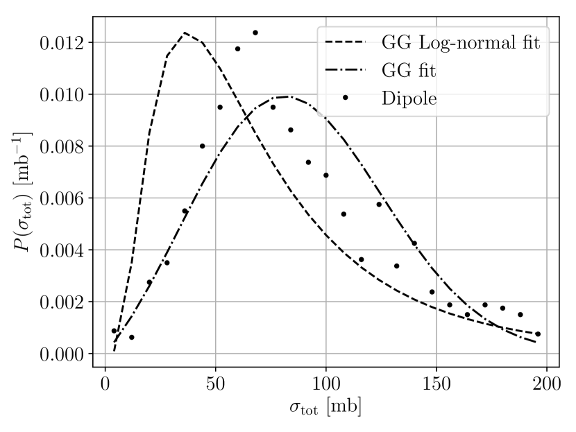
Fluctuations in the pp cross sections, to estimate the influence of fluctuations in collisions, are often parametrized using Heiselberg:1991is ; Blaettel:1993ah ; Goncalves:2019agu :
| (47) |
where and are parameters, and is a normalization constant. In ref. Bierlich:2016smv is was found that a log-normal distribution (see eq. (84) in appendix B) describes fluctuations generated by a dipole approach better. In figure 16 (a) both parametrizations are compared to the fluctuating total cross section in pp at 5 TeV, integrated over .
(a)
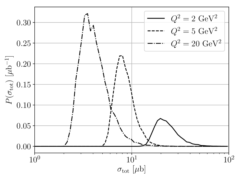
(b)
While the log-normal distribution does better in capturing the skewness of the distribution, none of the two parametrizations fully describes the distribution. The problem increases in for several reasons. First of all, any parametrization must include the correct dependence on DIS kinematics, which changes the average cross section, cf. figure 16 (b). Here is shown the cross section distributions for three values of all with GeV2 with a logarithmic first axis. This allows for a by-eye assessment of the validity of a log-normal fit, as a log-normal distribution is Gaussian with such choice of axes. It is seen directly that fluctuations in the high- tails are too large to be described by such a parametrization.
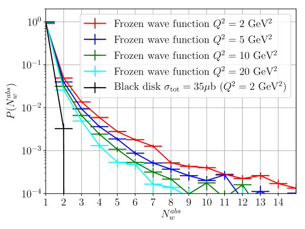
Instead of the parametrization approach, the wounded cross section can be calculated directly from the dipole evolution. This also allows for simultaneous calculation of both the part including electromagnetic contributions, and the pure dipole part (given and ), as introduced in the previous section. This allows directly for a calculation of the distribution of wounded nucleons in a collision, as shown in figure 17. In the figure, the nucleus is taken to be Au-197, colliding with a virtual photon with GeV2 for a range of values, compatible with projected EIC design Accardi:2012qut . Two methods of calculating wounded nucleons are presented: the full treatment using a frozen wave function, where the photon wave function has collapsed to a dipole state when probed by the first collision, and the naive black disk approach, where the photon re-forms after the full collision and no fluctuations are included. In such a treatment, the cross section for additional collisions has an additional factor compared to the frozen treatment, from the normalization of the wave function. It is directly visible that a full treatment is necessary in order to provide reasonable phenomenological projections for a new collider.
8 Conclusion and outlook
One of the main challenges for the understanding of collective effects, is to grasp how the well-known understanding of flow results from heavy ion collisions can be transferred to collision of protons with protons and heavy nuclei. In this paper we have presented a Monte Carlo implementation of Mueller’s dipole model with several sub-leading corrections, and with all parameters of the model fixed to total and semi-inclusive cross sections calculated within the Good-Walker formalism. This model thus allows for the calculation of proton substructure without tuning any model parameters to observables sensitive to said substructure.
The current implementation of the model includes:
-
•
BFKL evolution of projectile and target states, be it protons or photons, in rapidity and impact parameter space.
-
•
Sub-leading corrections in the evolution:
-
1.
Energy-momentum conservation.
-
2.
Non-eikonal corrections in terms of dipole recoils.
-
3.
Confinement effects by the introduction of a fictitious gluon mass.
-
1.
-
•
Projectile–target interactions using the unitarized amplitude, which in a Regge field theory language corresponds to multi-Pomeron exchange and Pomeron loops.
-
•
Matching to the Pythia 8 MPI model, in order to assign spatial vertices to produced partons in collisions.
-
•
Generalization to heavy ion collisions through the Angantyr framework.
Besides the implementation of the dipole model, a simpler version has been provided, based on the geometric properties of the dipole evolution. This model, denoted the Pascal approximation, allows for easy insertion of toy-models of sub-leading effects, thus giving a handle on the importance of such effects.
We have shown that given simple, but reasonable, assumptions of a final–state response (from e.g. hydrodynamics or interacting strings), the eccentricities produced with the implementation provides a reasonable description of flow data from the ALICE and CMS experiments. This includes non-trivial observations such as ratios between and flow coefficients at fixed event multiplicity, normalized symmetric cumulants in different systems, and ratios between different order flow harmonics in collisions. All are signatures which cannot be described in a simpler model, where the spatial structure of MPIs are assumed to be distributed according to a rotationally symmetric distribution. We want to stress that even though we have here chosen flow-type observables to illustrate the effect of the space-time structure of the initial state on observations of collective effects, effects linked to enhancement of strangeness and baryon production Biro:1984cf ; Bierlich:2014xba ; Bierlich:2015rha and even modifications of jets in high multiplicity pp collisions Mangano:2017plv ; Bierlich:2019ixq are expected to be influenced as well.
Lastly, we have provided the initial steps towards the generation of
fully exclusive final states in electron-ion collisions, by
determining the importance of colour-fluctuations in the collisions with
virtual photons. We have shown that previous parametrizations from
collisions do not fully capture the colour-fluctuations predicted
by the dipole formulation of BFKL evolution, and thus argue that it is better to calculate the
cross sections directly from the dipole model – which has not been
possible in the Angantyr model before this work. Secondly, we
stress that the collapse of the photon wave function at first interaction
provides a larger number of wounded nucleons as compared to the black
disk approximation. Each of the wounded nucleons are expected to give
rise to final state activity, thus more complicated final states are
expected with the proper treatment as opposed to the naive
expectations.
The implemented dipole model can be improved in several ways, including:
-
•
Running in the dipole evolution and in the scattering, which will capture some of the NLO corrections in .
-
•
On longer term, an inclusion of full NLO-BK should be the goal, though further theoretical development is needed first.
-
•
Gluon saturation effects in the cascade such as those included in the CGC formalism. To maintain the current treatment of the effect of gluon branchings in the cascade (as opposed to CGC), this could be included by the introduction of a simple swing mechanism, e.g. a mock dipole recombination.
-
•
Several improvements are expected w.r.t. the initial dipole configuration in protons and photons, as well as in the wave functions of these particles. This includes adding the VMD contribution to the photon wave function, to be able to study lower and vector meson production in various processes.
-
•
New ways of treating MPIs in collisions by fully merging the dipole approach with more traditional approaches are foreseen. It is our hope that this could provide new tools to improve understanding of particle production mechanisms across collision systems.
Detailed understanding of the interplay between the proton geometry and the response of final state interactions in hadronic and heavy ion collisions, is crucial for the understanding of collectivity and particle production mechanisms. Since detailed understanding requires tools which are both accessible and transparent, it is our hope that the detailed treatment presented here, and the accompanying open Monte Carlo implementation, can help facilitate this process.
Acknowledgements.
We thank Gösta Gustafson, Leif Lönnblad and Torbjörn Sjöstrand for several discussions during the making of this project and Gösta, Torbjörn and Helen Brooks for reading through and commenting on the manuscript. We also thank the ALICE group at the Niels Bohr Institute, University of Copenhagen for hospitality during the writing of this work. This project has received funding in part from the European Research Council (ERC) under the European Union’s Horizon 2020 research and innovation program (grant agreement No 668679), and in part by the Swedish Research Council, contract numbers 2016-05996 and 2017-0034 as well as the Marie Skłodowska-Curie Innovative Training Network MCnetITN3 (grant agreement 722104).Appendix A Appendix: The dipole model
We here work with light cone momenta,
| (48) |
and can thus define the rapidity as
| (49) |
with the latter equality valid for massless particles. Hence we can express the lightcone momenta in terms of dipole and rapidity,
| (50) |
The of a dipole can be related to its size through .
The dipole-dipole scatterings are defined to occur at rapidity zero. Thus the evolution of the beams begin at rapidity and evolve to zero, i.e. with negative rapidity steps. For technical reasons, the actual evolution is easier to implement with positive steps in rapidity. Thus the internal rapidity used in the code (and in the next section) is negated w.r.t. the rapidity defined in eq. (49):
| (51) | ||||
| (52) |
where in the forthcoming sections we will skip the subscript .
A.1 Mueller’s dipole branching
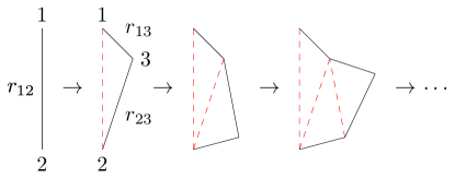
We begin by examining the dipole splitting function,
| (53) |
where is the transverse location of the emitted parton from the original dipole spanned by partons and the length of the dipoles, also shown in figure 18. In order to turn this into a dipole evolution, a Sudakov factor, , restricting emission between and , has to be introduced. The full dipole splitting kernel then reads,
| (54) |
For event generation to proceed, we need to find an overestimate for the above splitting probability. The Sudakov factor is included via the veto algorithm, and is thus neglected in the expressions below.
First we sample a transverse location of the emitting dipole. Assuming partons 1 and 2 located in the -plane at and with length fm, while the emitted parton is located at , we can write the splitting probability as,
| (55) |
where in the second step we have inserted the values for fm
and fm2, but suppressed dimensions. These dimensions are
suppressed throughout the section.
This distribution is symmetric around fm and fm, so the
limits of integration can be changed from to
and .
The above splitting probability can be overestimated by the function,
| (56) |
Changing to cylindrical coordinates we obtain,
| (57) |
which can be integrated from a minimal dipole size, . Thus we obtain,
| (58) |
Without energy ordering, the minimal dipole size has to be fixed to a number larger than zero to avoid the distribution from blowing up. Here, energy the ordering is introduced by ordering of positive lightcone momenta Avsar:2005iz . Again relating the transverse momentum of the dipole to its size, gives an expression for related to the kinematics of the parent dipole (),
| (59) |
This expression is then used in eq. (58),
| (60) |
This overestimate cannot trivially be integrated, so we find yet another,
| (61) |
which is both integrable and invertible. We take into account the Sudakov factor by using the Veto algorithm, and thus the rapidity can be sampled from this distribution by
| (62) |
where is a uniformly distributed random number.
From eq. (58) we can sample both and ,
| (63) | ||||
| (64) |
with two new random numbers. Here we should note that we’ve changed the integration limits, such that any must be rejected in the event generation. Half of the remaining events should be mirrored to , and this should be taken into account in the overestimate as well, such that
| (65) |
The events are weighted to the correct distributions with,
| (66) | ||||
| (67) |
such that if the event is rejected and the process is reiterated.
The evolution of an initial dipole thus goes as follows. Firstly, a trial emission from the initial dipole is performed according to eq. (53). If the rapidity of this emission is below the maximally allowed rapidity, then the trial branching is accepted, thus two new dipoles are created. Trial emissions are then allowed from each of these dipoles using in eq. (53). This creates two new emissions with rapidities . But here only the dipole with the smallest rapidity is accepted. Thus after the second iteration we have three dipoles, from each of which trial emissions are created and only the emission with the smallest rapidity is accepted, thus creating an additional dipole. The process is reiterated until no trial emissions are produced below the maximally allowed rapidity. The process is visualized in figure 18.
The choice of of the emitted parton is not obvious. Here we assign the parton the largest of the system,
| (68) |
A.1.1 Ordering of lightcone momenta
We here rely on approximate energy conservation through ordering of . This has already been discussed in the above, where we found the cutoff for small dipoles in the event generation of , eq. (59). Thus we have implemented energy conservation as
| (69) |
which implies a rapidity-dependent cutoff for smaller dipoles.
Momentum conservation is introduced through the ordering of ,
| (70) |
where it should be noted that this requirement is applied after the recoils have been taken into account. This choice also sets an upper bound for the dipole size through
| (71) |
A.1.2 Recoil effects
The recoil of the emitted parton is shared equally between the partons spanning the emitting dipole. Energy conservation requires that the energy of the emitter after the emission of a new dipole equals the energy of the emitter before the collision minus the recoil,
| (72) |
The recoil cannot be determined from first principles thus have to make an ansatz. The choice here is also from Avsar:2005iz ,
| (73) |
thus the recoil on parton depends on the length of the dipole spanned by partons 2, 3 and vice versa. Energy conservation is satisfied in the event generation by always requiring that .
The recoil will also affect the of the emitter. Here the choice is
| (74) |
where are the initial partons and is the emitted parton.
Changing both the and of the emitter thus also requires us to change the rapidity of the emitter for consistency,
| (75) |
Note here that the rapidity of the parent after the recoil will always be larger than the rapidity of the parent dipole before the recoil. This is because after the recoil is always smaller than before the recoil, while the is after the recoil is always larger than or equal to the before the recoil. Because of this, we must require that the rapidity of the emitters after the recoil is smaller than the rapidity of the emitted gluon, .
A.1.3 Effects of confinement
Here it should be noted that the modified Bessel functions behave as for small arguments, while falling off exponentially at large arguments, . Thus the confined distribution is overestimated by the unconfined distribution, and the introduction of confinement only adds an additional weight that vetoes events with large dipole sizes.
A.2 Initial states
The initial dipole configuration depends on the particle. Here we present two types: a proton sampler and a photon sampler. The difference here lies both in the number of initial dipoles (three for protons, one for photons) and in the wave function of the particle itself.
A.2.1 Protons
The initial state proton is not known from QCD, but instead has to be described by some phenomenological model. At rest, it consists primarily of three valence quarks, which we can view as endpoints of the initial dipoles. The configuration of these dipoles, however, is not known, thus we here work with a single scenario: An equilateral triangle.
We allow the dipole length to be distributed according to a Gaussian of mean and width , such that the length of the initial dipoles is given as:
| (76) |
with a Gaussian random number. The center of the triangle is fixed at origo.
A.2.2 Photons
The wave function used in this work is presented in eqs. (22–23). The full cross section for is then given as
| (77) |
with the dipole-dipole scattering cross sections given in equations (11-13). The dipole-dipole scattering cross section goes roughly as the square of the size of the largest dipole, , thus an overestimate of the cross section can be found by sampling the parameters from the following distributions, we obtain
| (78) | ||||
| (79) | ||||
| (80) | ||||
| (81) |
The maximal value obtained in the sum is kept to accept or reject the integrand in the algorithm, where first and are chosen and then accepted w.r.t.
| (82) |
If this weight is less than a new random number, , the event is rejected. If kept, the event is given a weight to take into account the overestimation of the dipole-dipole scattering cross section.
Appendix B Appendix: The Angantyr model for heavy ion collisions
The Angantyr model for heavy ion collisions is based on the following four components:
-
•
Firstly, the position of the nucleons inside the nuclei has to be determined.
-
•
Secondly, the number of interacting nucleons and binary collisions has to be calculated within the Glauber-Gribov (GG) formalism.
-
•
Thirdly, the contribution to the final state of each interacting nucleon has to be determined. Here Angantyr uses the wounded nucleon model by Białas, Bleszyński and Czyż Bialas:1976ed .
-
•
Lastly, any hard partonic subcollision has to be modeled, thus introducing the concepts of primary and secondary absorptive interactions.
Each of the four components will here be shortly reviewed. For the full explanation, see Bierlich:2016smv ; Bierlich:2018xfw .
The nucleon distribution is generated using a Woods-Saxon potential:
| (83) |
with the radial density of the nucleons, the radius of the nucleus, the skin width and the Fermi parameter, introducing a varying density but set to zero in Angantyr. The nucleons are thus generated randomly according to , assuming isospin invariance, such that . Angantyr uses the hard core assumption, such that a new position for a nucleus is tried if the distance to its neighbours falls below twice the hard-core radius . Once the nuclear distributions are set up, the impact parameter of the collision is sampled using a Gaussian distribution. This information is then passed the GG framework, which determines the fluctuations of the target and projectiles.
The fluctuations arise because of fluctuations in the proton wave function. Because the wave function enters in the cross section calculations and because it is assumed that the projectile state is frozen during its interaction with the target, these fluctuation are then translated into fluctuating cross sections. In the dipole model, the probabilistic nature of the dipole evolution gives rise to different dipole configurations before the collisions, thus giving rise to different dipole-dipole interactions and hence integrated cross sections. Angantyr uses a probability distribution for the cross section in extracted from Dipsy:
| (84) | ||||
| (85) |
with and eq. (85) describing a slightly modified version of the elastic scattering amplitude. The parameters are tuned to data. For the fluctuations are instead determined by a Gamma function,
| (86) | ||||
| (87) | ||||
| (88) |
where determines fluctuations in the nucleon radius and . again describes a slightly modified elastic amplitude with an opacity depending on the radii of both the target and projectile. Here, the parameters are tuned to data. The number of wounded target nucleons in collisions is then determined by
| (89) |
with the S-matrix for a given target () and projectile () state. Subscript on the brackets determines averages over one side only. In collisions Angantyr distinguishes between absorptively and diffractively wounded nucleons, with the former dominating given by,
| (90) |
and the latter determined by generating the auxiliary states for both target and projectile, and from these determining the number of wounded target states with either or from eq. (89), i.e. using either or in the derivation. Non-negative probabilities are ensured by shuffling when to use .
Once the number of wounded target and projectile states has been determined, the wounded nucleon model is used to create final-state partons,
| (91) |
with the functions determined from the MPI framework of Pythia 8. Each nucleon in the target (and projectile) is allowed to interact several times, similar to an ordinary collision containing several MPIs. Thus the pairs of projectile-target nucleons are ordered w.r.t. their impact-parameter . The list is iterated over several times in order to determine which pairs give rise to a primary absorptive scattering, and which are secondary. Once a pair has been selected, the MPI framework of Pythia 8 is used to generate an event, and the pair is marked as having interacted in a primary interaction. If the pair is again chosen to interact, it will be marked as a secondary interaction. After the determination of the absorptive interactions, the diffractive ones are chosen by iterating the list several times, thus creating primary and secondary diffractive interactions. An already wounded nucleon cannot be further excited, but an unwounded nucleon can participate in several diffractive interactions, until itself becomes wounded.
After the determination of the absorptive and diffractively primary and secondary interactions, each of the events are passed to Pythia 8 and the parton-level events are stacked on top of each other. The Pythia 8 description of single-diffractive events are modified to look like non-diffractive ones, to describe the secondary absorptive events, while diffractive primary and secondary events remain unmodified. We are thus left with a large set of parton-level events that can be passed to the hadronisation framework of Pythia 8 and further analysed.
Appendix C Appendix: Additional eccentricity figures
In this section, we show additional eccentricity figures not presented in the main body of the text. Figure 19 (a-c) shows using higher-order cumulants in the evaluation. It is evident that the eccentricities are the same regardless of the number of particles used in the calculation, except for the effects from lack of statistics in the high-multiplicity tail for both the and figures. Figure 19 (d) shows the normalized symmetric cumulant . This cumulant is positive in the entire multiplicity range, consistent with measurements in ALICE. Here, it is evident that discrimination between models would be possible in both and collisions, as opposed to where discriminatory power was not evident in collisions.
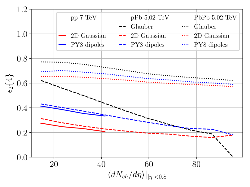
(a)
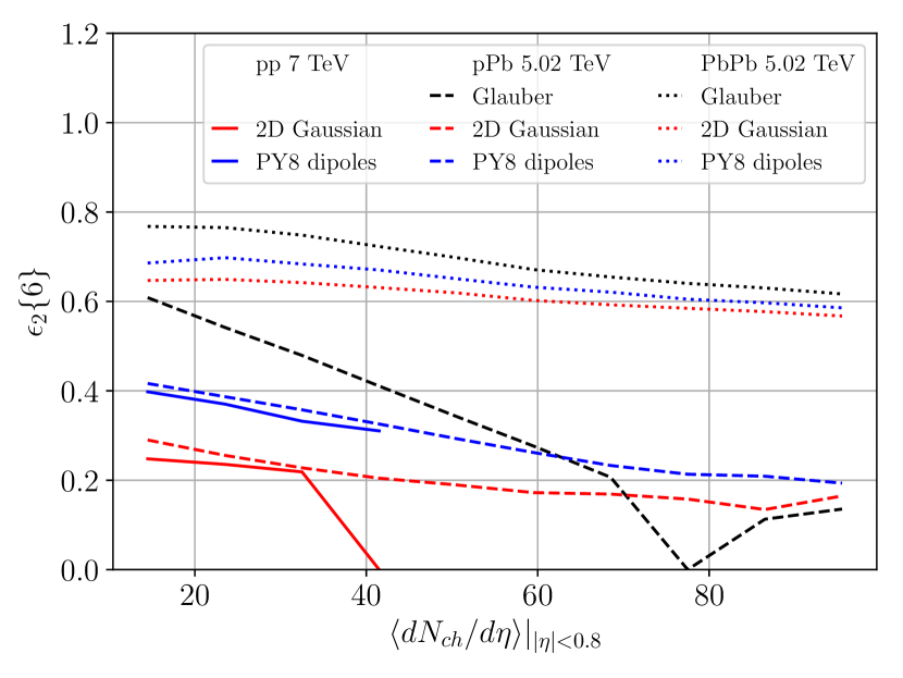
(b)
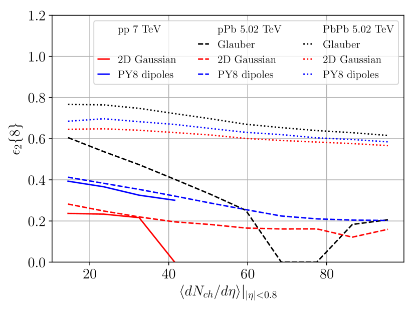
(c)
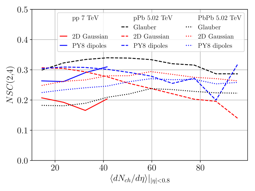
(d)
For completeness, we also show the eccentricities obtained in collisions with and without shower smearing in figure 20. Both are shown to give an estimate of the effects on the size of the additional terms in the Fourier expansion of the flow coefficients.
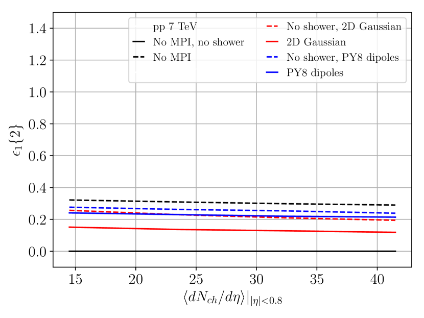
(a)
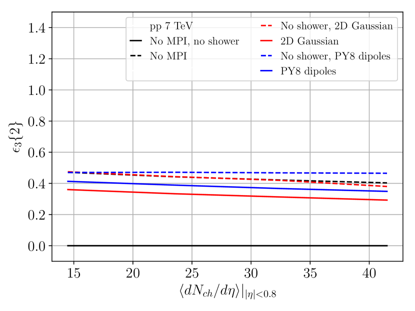
(b)
References
- (1) STAR collaboration, K. H. Ackermann et al., Elliptic flow in Au + Au collisions at ( = 130 GeV, Phys. Rev. Lett. 86 (2001) 402 [nucl-ex/0009011].
- (2) ALICE collaboration, K. Aamodt et al., Elliptic flow of charged particles in Pb-Pb collisions at 2.76 TeV, Phys. Rev. Lett. 105 (2010) 252302 [1011.3914].
- (3) CMS collaboration, S. Chatrchyan et al., Long-range and short-range dihadron angular correlations in central PbPb collisions at a nucleon-nucleon center of mass energy of 2.76 TeV, JHEP 07 (2011) 076 [1105.2438].
- (4) ATLAS collaboration, G. Aad et al., Measurement of the azimuthal anisotropy for charged particle production in TeV lead-lead collisions with the ATLAS detector, Phys. Rev. C86 (2012) 014907 [1203.3087].
- (5) J.-Y. Ollitrault, Anisotropy as a signature of transverse collective flow, Phys. Rev. D46 (1992) 229.
- (6) V. A. Abramovskiĭ, E. V. Gedalin, E. G. Gurvich and O. V. Kancheli, Long Range Azimuthal Correlations in Multiple Production Processes at High-energies, JETP Lett. 47 (1988) 337.
- (7) CMS collaboration, S. Chatrchyan et al., Observation of Long-Range Near-Side Angular Correlations in Proton-Lead Collisions at the LHC, Phys. Lett. B718 (2013) 795 [1210.5482].
- (8) PHENIX collaboration, C. Aidala et al., Measurements of Multiparticle Correlations in Collisions at 200, 62.4, 39, and 19.6 GeV and Collisions at 200 GeV and Implications for Collective Behavior, Phys. Rev. Lett. 120 (2018) 062302 [1707.06108].
- (9) CMS collaboration, V. Khachatryan et al., Observation of Long-Range Near-Side Angular Correlations in Proton-Proton Collisions at the LHC, JHEP 09 (2010) 091 [1009.4122].
- (10) A. Badea, A. Baty, P. Chang, G. M. Innocenti, M. Maggi, C. McGinn et al., Measurements of two-particle correlations in collisions at 91 GeV with ALEPH archived data, 1906.00489.
- (11) J. L. Nagle and W. A. Zajc, Small System Collectivity in Relativistic Hadronic and Nuclear Collisions, Ann. Rev. Nucl. Part. Sci. 68 (2018) 211 [1801.03477].
- (12) Z. Citron et al., Future physics opportunities for high-density QCD at the LHC with heavy-ion and proton beams, in HL/HE-LHC Workshop: Workshop on the Physics of HL-LHC, and Perspectives at HE-LHC Geneva, Switzerland, June 18-20, 2018, 2018, 1812.06772.
- (13) B. Blok, C. D. Jäkel, M. Strikman and U. A. Wiedemann, Collectivity from interference, JHEP 12 (2017) 074 [1708.08241].
- (14) K. Dusling and R. Venugopalan, Explanation of systematics of CMS p+Pb high multiplicity di-hadron data at TeV, Phys. Rev. D87 (2013) 054014 [1211.3701].
- (15) R. D. Weller and P. Romatschke, One fluid to rule them all: viscous hydrodynamic description of event-by-event central p+p, p+Pb and Pb+Pb collisions at TeV, Phys. Lett. B774 (2017) 351 [1701.07145].
- (16) K. Werner, Core-corona separation in ultra-relativistic heavy ion collisions, Phys. Rev. Lett. 98 (2007) 152301 [0704.1270].
- (17) T. Pierog, I. Karpenko, J. M. Katzy, E. Yatsenko and K. Werner, EPOS LHC: Test of collective hadronization with data measured at the CERN Large Hadron Collider, Phys. Rev. C92 (2015) 034906 [1306.0121].
- (18) T. Sjöstrand, S. Ask, J. R. Christiansen, R. Corke, N. Desai, P. Ilten et al., An Introduction to PYTHIA 8.2, Comput. Phys. Commun. 191 (2015) 159 [1410.3012].
- (19) J. Bellm et al., Herwig 7.0/Herwig++ 3.0 release note, Eur. Phys. J. C76 (2016) 196 [1512.01178].
- (20) D. d’Enterria, G. K. Eyyubova, V. L. Korotkikh, I. P. Lokhtin, S. V. Petrushanko, L. I. Sarycheva et al., Estimates of hadron azimuthal anisotropy from multiparton interactions in proton-proton collisions at TeV, Eur. Phys. J. C66 (2010) 173 [0910.3029].
- (21) J. L. Albacete and A. Soto-Ontoso, Hot spots and the hollowness of proton–proton interactions at high energies, Phys. Lett. B770 (2017) 149 [1605.09176].
- (22) C. Bierlich, G. Gustafson and L. Lönnblad, Collectivity without plasma in hadronic collisions, Phys. Lett. B779 (2018) 58 [1710.09725].
- (23) A. H. Mueller, Soft gluons in the infinite momentum wave function and the BFKL pomeron, Nucl. Phys. B415 (1994) 373.
- (24) A. H. Mueller and B. Patel, Single and double BFKL pomeron exchange and a dipole picture of high-energy hard processes, Nucl. Phys. B425 (1994) 471 [hep-ph/9403256].
- (25) E. Avsar, C. Flensburg, Y. Hatta, J.-Y. Ollitrault and T. Ueda, Eccentricity and elliptic flow in proton–proton collisions from parton evolution, Phys. Lett. B702 (2011) 394 [1009.5643].
- (26) I. Balitsky, Operator expansion for high-energy scattering, Nucl. Phys. B463 (1996) 99 [hep-ph/9509348].
- (27) I. Balitsky, Factorization for high-energy scattering, Phys. Rev. Lett. 81 (1998) 2024 [hep-ph/9807434].
- (28) I. Balitsky, Effective field theory for the small x evolution, Phys. Lett. B518 (2001) 235 [hep-ph/0105334].
- (29) J. Jalilian-Marian, A. Kovner, A. Leonidov and H. Weigert, The BFKL equation from the Wilson renormalization group, Nucl. Phys. B504 (1997) 415 [hep-ph/9701284].
- (30) J. Jalilian-Marian, A. Kovner, A. Leonidov and H. Weigert, The Wilson renormalization group for low x physics: Towards the high density regime, Phys. Rev. D59 (1998) 014014 [hep-ph/9706377].
- (31) E. Iancu, A. Leonidov and L. D. McLerran, The Renormalization group equation for the color glass condensate, Phys. Lett. B510 (2001) 133 [hep-ph/0102009].
- (32) E. Iancu, A. Leonidov and L. D. McLerran, Nonlinear gluon evolution in the color glass condensate. 1., Nucl. Phys. A692 (2001) 583 [hep-ph/0011241].
- (33) H. Weigert, Unitarity at small Bjorken x, Nucl. Phys. A703 (2002) 823 [hep-ph/0004044].
- (34) M. Deak, K. Kutak, W. Li and A. M. Staśto, On the different forms of the kinematical constraint in BFKL, 1906.09062.
- (35) C. Bierlich, G. Gustafson and L. Lönnblad, Diffractive and non-diffractive wounded nucleons and final states in pA collisions, JHEP 10 (2016) 139 [1607.04434].
- (36) C. Bierlich, G. Gustafson, L. Lönnblad and H. Shah, The Angantyr model for Heavy-Ion Collisions in PYTHIA8, JHEP 10 (2018) 134 [1806.10820].
- (37) A. Accardi et al., Electron Ion Collider: The Next QCD Frontier, Eur. Phys. J. A52 (2016) 268 [1212.1701].
- (38) G. P. Salam, OEDIPUS: Onium evolution, dipole interaction and perturbative unitarization simulation, Comput. Phys. Commun. 105 (1997) 62 [hep-ph/9601220].
- (39) E. Avsar, G. Gustafson and L. Lönnblad, Energy conservation and saturation in small-x evolution, JHEP 07 (2005) 062 [hep-ph/0503181].
- (40) C. Flensburg, G. Gustafson and L. Lönnblad, Inclusive and Exclusive Observables from Dipoles in High Energy Collisions, JHEP 08 (2011) 103 [1103.4321].
- (41) V. Kovalenko and V. Vechernin, Model of pp and AA collisions for the description of long-range correlations, PoS Baldin-ISHEPP-XXI (2012) 077 [1212.2590].
- (42) E. Avsar, G. Gustafson and L. Lönnblad, Diifractive excitation in DIS and collisions, JHEP 12 (2007) 012 [0709.1368].
- (43) E. Avsar, On the dipole swing and the search for frame independence in the dipole model, JHEP 11 (2007) 027 [0709.1371].
- (44) B. Schenke, P. Tribedy and R. Venugopalan, Fluctuating Glasma initial conditions and flow in heavy ion collisions, Phys. Rev. Lett. 108 (2012) 252301 [1202.6646].
- (45) A. H. Mueller, A Simple derivation of the JIMWLK equation, Phys. Lett. B523 (2001) 243 [hep-ph/0110169].
- (46) E. A. Kuraev, L. N. Lipatov and V. S. Fadin, The Pomeranchuk Singularity in Nonabelian Gauge Theories, Sov. Phys. JETP 45 (1977) 199.
- (47) I. I. Balitsky and L. N. Lipatov, The Pomeranchuk Singularity in Quantum Chromodynamics, Sov. J. Nucl. Phys. 28 (1978) 822.
- (48) Y. V. Kovchegov, Small x F(2) structure function of a nucleus including multiple pomeron exchanges, Phys. Rev. D60 (1999) 034008 [hep-ph/9901281].
- (49) E. Iancu and R. Venugopalan, The Color glass condensate and high-energy scattering in QCD, in Quark-gluon plasma 4 (R. C. Hwa and X.-N. Wang, eds.), pp. 249–3363. World Scientific, 2003. hep-ph/0303204. DOI.
- (50) F. Gelis, E. Iancu, J. Jalilian-Marian and R. Venugopalan, The Color Glass Condensate, Ann. Rev. Nucl. Part. Sci. 60 (2010) 463 [1002.0333].
- (51) I. Balitsky, High-energy QCD and Wilson lines, hep-ph/0101042.
- (52) F. Close, S. Donnachie and G. Shaw, Electromagnetic interactions and hadronic structure, Camb. Monogr. Part. Phys. Nucl. Phys. Cosmol. 25 (2007) 1.
- (53) A. M. Staśto, K. J. Golec-Biernat and J. Kwiecinski, Geometric scaling for the total p cross-section in the low x region, Phys. Rev. Lett. 86 (2001) 596 [hep-ph/0007192].
- (54) Y. V. Kovchegov and E. Levin, Quantum chromodynamics at high energy, Camb. Monogr. Part. Phys. Nucl. Phys. Cosmol. 33 (2012) 1.
- (55) I. Balitsky and G. A. Chirilli, Next-to-leading order evolution of color dipoles, Phys. Rev. D77 (2008) 014019 [0710.4330].
- (56) A. Kovner, M. Lublinsky and Y. Mulian, Jalilian-Marian, Iancu, McLerran, Weigert, Leonidov, Kovner evolution at next to leading order, Phys. Rev. D89 (2014) 061704 [1310.0378].
- (57) A. Kovner, M. Lublinsky and Y. Mulian, NLO JIMWLK evolution unabridged, JHEP 08 (2014) 114 [1405.0418].
- (58) M. Lublinsky and Y. Mulian, High Energy QCD at NLO: from light-cone wave function to JIMWLK evolution, JHEP 05 (2017) 097 [1610.03453].
- (59) T. Lappi and H. Mäntysaari, Direct numerical solution of the coordinate space Balitsky-Kovchegov equation at next to leading order, Phys. Rev. D91 (2015) 074016 [1502.02400].
- (60) B. Ducloué, E. Iancu, A. H. Mueller, G. Soyez and D. N. Triantafyllopoulos, Non-linear evolution in QCD at high-energy beyond leading order, JHEP 04 (2019) 081 [1902.06637].
- (61) E. Avsar, G. Gustafson and L. Lönnblad, Small-x dipole evolution beyond the large-N(c) imit, JHEP 01 (2007) 012 [hep-ph/0610157].
- (62) G. Beuf, Improving the kinematics for low- QCD evolution equations in coordinate space, Phys. Rev. D89 (2014) 074039 [1401.0313].
- (63) V. S. Fadin and L. N. Lipatov, BFKL pomeron in the next-to-leading approximation, Phys. Lett. B429 (1998) 127 [hep-ph/9802290].
- (64) M. Ciafaloni and G. Camici, Energy scale(s) and next-to-leading BFKL equation, Phys. Lett. B430 (1998) 349 [hep-ph/9803389].
- (65) G. P. Salam, An Introduction to leading and next-to-leading BFKL, Acta Phys. Polon. B30 (1999) 3679 [hep-ph/9910492].
- (66) T. Altinoluk, N. Armesto, G. Beuf, M. Martínez and C. A. Salgado, Next-to-eikonal corrections in the CGC: gluon production and spin asymmetries in pA collisions, JHEP 07 (2014) 068 [1404.2219].
- (67) H. Niemi, G. S. Denicol, H. Holopainen and P. Huovinen, Event-by-event distributions of azimuthal asymmetries in ultrarelativistic heavy-ion collisions, Phys. Rev. C87 (2013) 054901 [1212.1008].
- (68) C. Bierlich, G. Gustafson and L. Lönnblad, A shoving model for collectivity in hadronic collisions, 1612.05132.
- (69) Z. Qiu and U. W. Heinz, Event-by-event shape and flow fluctuations of relativistic heavy-ion collision fireballs, Phys. Rev. C84 (2011) 024911 [1104.0650].
- (70) Y. Zhou, Anisotropic Flow and Flow Fluctuations at the Large Hadron Collider, Ph.D. thesis, Utrecht U., 2016.
- (71) J. L. Albacete, H. Petersen and A. Soto-Ontoso, Symmetric cumulants as a probe of the proton substructure at LHC energies, Phys. Lett. B778 (2018) 128 [1707.05592].
- (72) E. Avsar and G. Gustafson, Geometric scaling and QCD dynamics in DIS, JHEP 04 (2007) 067 [hep-ph/0702087].
- (73) A. H. Mueller and G. P. Salam, Large multiplicity fluctuations and saturation effects in onium collisions, Nucl. Phys. B475 (1996) 293 [hep-ph/9605302].
- (74) T. Sjöstrand and M. van Zijl, A Multiple Interaction Model for the Event Structure in Hadron Collisions, Phys. Rev. D36 (1987) 2019.
- (75) T. Sjöstrand and P. Z. Skands, Multiple interactions and the structure of beam remnants, JHEP 03 (2004) 053 [hep-ph/0402078].
- (76) A. Donnachie and P. V. Landshoff, Total cross-sections, Phys. Lett. B296 (1992) 227 [hep-ph/9209205].
- (77) G. A. Schuler and T. Sjöstrand, Hadronic diffractive cross-sections and the rise of the total cross-section, Phys. Rev. D49 (1994) 2257.
- (78) R. B. Appleby, R. J. Barlow, J. G. Molson, M. Serluca and A. Toader, The Practical Pomeron for High Energy Proton Collimation, Eur. Phys. J. C76 (2016) 520 [1604.07327].
- (79) C. O. Rasmussen and T. Sjöstrand, Models for total, elastic and diffractive cross sections, Eur. Phys. J. C78 (2018) 461 [1804.10373].
- (80) H1 collaboration, C. Adloff et al., Deep inelastic inclusive ep scattering at low x and a determination of alpha(s), Eur. Phys. J. C21 (2001) 33 [hep-ex/0012053].
- (81) A. Buckley, H. Hoeth, H. Lacker, H. Schulz and J. E. von Seggern, Systematic event generator tuning for the LHC, Eur. Phys. J. C65 (2010) 331 [0907.2973].
- (82) ALICE collaboration, S. Acharya et al., Investigations of anisotropic flow using multi-particle azimuthal correlations in pp, p-Pb, Xe-Xe, and Pb-Pb collisions at the LHC, 1903.01790.
- (83) CMS collaboration, A. M. Sirunyan et al., Multiparticle correlation studies in pPb collisions at 8.16 TeV, 1904.11519.
- (84) G. Giacalone, J. Noronha-Hostler and J.-Y. Ollitrault, Relative flow fluctuations as a probe of initial state fluctuations, Phys. Rev. C95 (2017) 054910 [1702.01730].
- (85) J. E. Bernhard, J. S. Moreland, S. A. Bass, J. Liu and U. Heinz, Applying Bayesian parameter estimation to relativistic heavy-ion collisions: simultaneous characterization of the initial state and quark-gluon plasma medium, Phys. Rev. C94 (2016) 024907 [1605.03954].
- (86) L. Yan and J.-Y. Ollitrault, Universal fluctuation-driven eccentricities in proton-proton, proton-nucleus and nucleus-nucleus collisions, Phys. Rev. Lett. 112 (2014) 082301 [1312.6555].
- (87) R. J. Glauber, Cross-sections in deuterium at high-energies, Phys. Rev. 100 (1955) 242.
- (88) M. L. Miller, K. Reygers, S. J. Sanders and P. Steinberg, Glauber modeling in high energy nuclear collisions, Ann. Rev. Nucl. Part. Sci. 57 (2007) 205 [nucl-ex/0701025].
- (89) M. Alvioli and M. Strikman, Color fluctuation effects in proton-nucleus collisions, Phys. Lett. B722 (2013) 347 [1301.0728].
- (90) H. Heiselberg, G. Baym, B. Blaettel, L. L. Frankfurt and M. Strikman, Color transparency, color opacity, and fluctuations in nuclear collisions, Phys. Rev. Lett. 67 (1991) 2946.
- (91) B. Blaettel, G. Baym, L. L. Frankfurt, H. Heiselberg and M. Strikman, Hadronic cross-section fluctuations, Phys. Rev. D47 (1993) 2761.
- (92) V. P. Gonçalves, R. P. da Silva and P. V. R. G. Silva, Diffractive excitation in and collisions at high energies, 1905.00806.
- (93) T. S. Biro, H. B. Nielsen and J. Knoll, Color Rope Model for Extreme Relativistic Heavy Ion Collisions, Nucl. Phys. B245 (1984) 449.
- (94) C. Bierlich, G. Gustafson, L. Lönnblad and A. Tarasov, Effects of Overlapping Strings in pp Collisions, JHEP 03 (2015) 148 [1412.6259].
- (95) C. Bierlich and J. R. Christiansen, Effects of color reconnection on hadron flavor observables, Phys. Rev. D92 (2015) 094010 [1507.02091].
- (96) M. L. Mangano and B. Nachman, Observables for possible QGP signatures in central pp collisions, Eur. Phys. J. C78 (2018) 343 [1708.08369].
- (97) C. Bierlich, Soft modifications to jet fragmentation in high energy proton–proton collisions, Phys. Lett. B795 (2019) 194 [1901.07447].
- (98) A. Białas, M. Bleszyński and W. Czyż, Multiplicity Distributions in Nucleus-Nucleus Collisions at High-Energies, Nucl. Phys. B111 (1976) 461.