Structure of resonance eigenfunctions for chaotic systems with partial escape

Abstract

Physical systems are often neither completely closed nor completely open, but instead they are best described by dynamical systems with partial escape or absorption. In this paper we introduce classical measures that explain the main properties of resonance eigenfunctions of chaotic quantum systems with partial escape. We construct a family of conditionally-invariant measures with varying decay rates by interpolating between the natural measures of the forward and backward dynamics. Numerical simulations in a representative system show that our classical measures correctly describe the main features of the quantum eigenfunctions: their multi-fractal phase space distribution, their product structure along stable/unstable directions, and their dependence on the decay rate. The (Jensen-Shannon) distance between classical and quantum measures goes to zero in the semiclassical limit for long- and short-lived eigenfunctions, while it remains finite for intermediate cases.

I Introduction.

Quantum chaos aims to relate observations in quantum systems to properties of the classical dynamics. Particularly interesting are the implications of the classically chaotic dynamics on the statistics of eigenvalues BohGiaSch1984 ; Ber1985 ; SieRic2001 ; MueHeuBraHaaAlt2004 and the distribution of eigenfunctions Vor1979 ; Ber1977b ; Ber1983 . In closed chaotic systems typical trajectories explore the phase space uniformly with respect to the Liouville measure. The quantum ergodicity theorem states that semiclassically almost all chaotic eigenfunctions converge to this measure Shn1974 ; CdV1985 ; Zel1987 ; ZelZwo1996 ; NonVor1998 ; BaeSchSti1998 ; Bie2001 .

Experimentally accessible physical systems are usually not closed and in many cases have a corresponding classical description in which trajectories escape or are absorbed. Such open systems appear, for example, in optical microcavities CaoWie2015 , nuclear reactions MitRicWei2010 , or microwave resonators Sto1999 . Classically, open systems are characterized by the coexistence of trapped and (transiently chaotic) escaping motion on the phase-space LaiTel2011 ; AltPorTel2013 . Quantum mechanically, one studies complex resonances using a quantum-scattering description Gas2014b . Chaotic resonance eigenfunctions show fractal distributions CasMasShe1999b and are not universally described by a single classical measure KeaNovPraSie2006 ; NonRub2007 .

Best understood are resonance eigenfunctions in open systems with full escape BorGuaShe1991 ; CasMasShe1999b ; SchTwo2004 ; KeaNovPraSie2006 ; NonRub2007 ; KeaNonNovSie2008 ; ErmCarSar2009 ; ClaKoeBaeKet2018 ; BilGarGeoGir2019 , in which particles are completely absorbed or escape to infinity. Examples are scattering systems (e.g., three-discs GasRic1989a ) and systems in which a phase-space region $\Omega\subset\Gamma$ acts as a leak AltPorTel2013 . Classically, a fractal chaotic saddle emerges as the set of points which never escape for times $t\rightarrow\pm\infty$. Typical (smooth) initial distributions converge towards a measure $\mu_{\text{nat}}$, the so-called natural measure, which is conditionally invariant (c-measure), decays with the characteristic natural decay rate $\gamma_{\text{nat}}$, and is smooth on the unstable manifold of the saddle PiaYor1979 ; DemYou2006 . Quantum mechanically, resonances are distributed according to a fractal Weyl law which is determined by the fractal dimension of the chaotic saddle Sjo1990 ; Lin2002 ; LuSriZwo2003 ; SchTwo2004 ; RamPraBorFar2009 ; EbeMaiWun2010 ; ErmShe2010 ; NonSjoZwo2014 . The phase-space structure of resonance eigenfunctions depends on their decay rate $\gamma$ KeaNovPraSie2006 and converges in the semiclassical limit to a c-measure NonRub2007 . For $\gamma_{\text{nat}}$ this limit is assumed to be the natural measure $\mu_{\text{nat}}$ CasMasShe1999b . For arbitrary decay rates a good description is given by conditionally invariant measures which are uniformly distributed on sets with the same temporal distance to the chaotic saddle ClaKoeBaeKet2018 .

Less understood are resonance eigenfunctions in open systems with partial escape, in which particles escape with some finite probability or their intensities are partially absorbed. These systems are used in the description of optical microcavities LeeRimRyuKwoChoKim2004 ; WieHen2008 ; WieMai2008 ; ShiWieCao2011 ; ShiHarFukHenSasNar2010 ; AltPorTel2013b ; HarShi2015 ; CaoWie2015 ; AltPorTel2015 ; KulWie2016 , where the intensity of light rays changes according to Fresnel’s law of reflection and transmission. Classically, such systems are again described by a natural c-measure $\mu_{\text{nat}}$, which is multifractal and supported on the full phase-space AltPorTel2013b . Quantum mechanically, the resonances have finite decay rates, do not follow a simple fractal Weyl law WieMai2008 ; NonSch2008 ; PotWeiBarKuhStoZwo2012 ; GutOsi2015 ; SchAlt2015 ; KoeMicBaeKet2013 , and the longest living resonances in fully chaotic optical microcavities are well described by $\mu_{\text{nat}}$ (also known as steady probability distribution) LeeRimRyuKwoChoKim2004 ; AltPorTel2013 ; HarShi2015 ; KulWie2016 . Further results were obtained for the relation to periodic orbits CarBenBor2016 ; PraCarBenBor2018 and the case of single channel openings LipRyuLeeKim2012 ; LipRyuKim2015 . However, there is no understanding of how the properties of resonance eigenfunctions depend on their decay rate.

In this paper we study the classical origin of the multifractal phase-space structure of resonance eigenfunctions in systems with partial escape. Long-lived eigenfunctions stretch along the unstable direction of the classical dynamics and are known to semiclassically correspond to the natural measure. Short-lived eigenfunctions stretch along the stable direction and we conjecture that they semiclassically correspond to the natural measure of the inverse classical dynamics. For increasing decay rates the main contribution changes continuously from unstable to stable direction. Combining both natural measures we introduce a family of c-measures which are uniform on sets with the same decay under forward and backward time evolution. Qualitatively, we find that these measures and resonance eigenfunctions have the same characteristic filamentary patterns on phase space and show a similar dependence on the decay rate. Quantitatively, we numerically support the conjecture for long- and short-lived eigenfunctions.

The paper is divided as follows. In Section II we numerically show the emergence of fractal phase-space distributions for resonance eigenfunctions in an exemplary system. In Sec. III we show how to construct a family of c-measures for all relevant decay rates. We then compare the resonance eigenfunctions with these measures in Sec. IV, qualitatively and quantitatively using information dimension and Jensen-Shannon divergence. A summary is given in Sec. V.

Figure 1: Eigenvalues and fractal eigenfunctions in a chaotic quantum map with partial escape. (a-c) Spectrum in $\gamma-\theta$ plane for (a) $h=1/250$, (b) $h=1/1\,000$ and (c) $h=1/4\,000$. Horizontal lines indicate classical decay rates $\gamma\in\{\gamma_{\text{nat}},\gamma_{\text{inv}},\gamma_{\text{max}}\}$ (from lower to upper: red, green, gray), defined in Sec. III. (d-f) Husimi phase-space distributions $\mathcal{H}_{\gamma}$ of single eigenfunction with decay rate closest to $\gamma=0.55$ for values of $h$ as in (a-c). (g-i) Average Husimi distributions $\langle\mathcal{H}\rangle_{\gamma}$ of eigenfunctions with decay rate in $(\gamma-\Delta\gamma,\gamma+\Delta\gamma)$ with $\gamma=0.55$ and $\Delta\gamma=0.016$ for values of $h$ as in (a-c), using $\{17,64,244\}$ eigenfunctions. Individual colormap for each $h$ with maximum given by $1.3\,\max\langle\mathcal{H}\rangle_{\gamma}$. Clear emergence of fractal structure. The system is the standard map, see App. A, on the torus $(q,p)\in[0,1)\times[0,1)$ with $\kappa=10$, reflection $R_{\Omega}=0.2$, and opening $\Omega=(0.3,0.6)\times[0,1)$ indicated by dashed lines in (d-i).

II Resonances in systems with partial escape

Scattering systems are described by the relation of incoming waves to outgoing waves, which is given by the $S$-matrix Gas2014b . Resonances appear as poles of the $S$-matrix and are experimentally seen as peaks in the absorption spectrum, whenever a resonance eigenfunction is excited. A similar description is found, if the dynamics is reducible to discrete times FyoSom2000 , e.g. in systems with time-periodical driving. In these systems the $S$-matrix takes the form KeaNovSch2008

$$S(\omega)=-\mathcal{R}+\mathcal{T}\frac{1}{\text{e}^{-\text{i}\omega}-\tilde{\mathcal{U}}\mathcal{R}}\tilde{\mathcal{U}}\mathcal{T},$$ (1)

with unitary time-evolution $\tilde{\mathcal{U}}$ of internal states and quasi-energy $\omega$. The internal reflection operator $\mathcal{R}$ and the transmission operator $\mathcal{T}$ govern the coupling from incoming to outgoing waves and satisfy $\mathcal{R}^{\dagger}\mathcal{R}+\mathcal{T}^{\dagger}\mathcal{T}=1$, which expresses the conservation of probability. Choosing an appropriate basis, the internal reflection $\mathcal{R}$ becomes diagonal with positive entries. E.g., for microresonators internal reflection is described by Fresnel’s law KeaNovSch2008 ; KulWie2016 . It follows from Eq. (1) that whenever $\text{e}^{-\text{i}\omega}$ is an eigenvalue of the operator

$$\mathcal{U}=\tilde{\mathcal{U}}\mathcal{R},$$ (2)

a resonance condition is fulfilled. The operator $\mathcal{U}$ describes the time-evolution of internal states composed of the reflection $\mathcal{R}$ and unitary time evolution $\tilde{\mathcal{U}}$. In the following $\mathcal{U}$ is called quantum map with escape. Solving the eigenvalue equation

$$\mathcal{U}\psi=\text{e}^{-\text{i}\theta-\gamma/2}\psi$$ (3)

gives the complex resonances $\omega=\theta-\text{i}\gamma/2$ and the (right) resonance eigenfunctions $\psi$. Note that in time-independent scattering systems $\theta$ corresponds to the energy and $\gamma$ to the width of the resonance. Applying the quantum map with escape (2) $n$-times to an eigenfunction $\psi$ the probability decays like $\|\mathcal{U}^{n}\psi\|^{2}=\text{e}^{-n\gamma}\|\psi\|^{2}$. Therefore $\gamma$ is called decay rate of the resonance eigenfunction $\psi$. Note that the quantization divides the compact phase space into an integer number of $1/h$ Planck cells, where $h$ is the effective Planck’s constant.

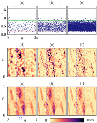
Figure 1 shows resonances and resonance eigenfunctions for a paradigmatic example of a chaotic quantum system with partial escape (the standard map, see Appendix A for details). There are two important observations:

• The spectra show that the resonances have finite decay rates $\gamma$, that are mostly inside a relatively narrow band, Fig. 1(a-c). The existence of spectral gaps NonSch2008 ; She2008 ; GutOsi2015 explains that the decay rates are away from zero and infinity. In particular, there exist decay rates $\gamma_{\text{nat}}$ and $\gamma_{\text{inv}}$ (explained in the next section) such that approximately $0<\gamma_{\text{nat}}\lesssim\gamma\lesssim\gamma_{\text{inv}}<\gamma_{\text{max}}$, where $\gamma_{\text{max}}$ is determined by the maximal allowed classical escape, Eq. (6) below.

• The main observation concerns the resonance eigenfunctions and will be explored and explained in greater generality in the remaining of the paper. Resonance eigenfunctions have a rich multifractal phase-space structure, Fig. 1(d-i). This structure is in contrast to the uniform distribution observed in closed chaotic systems. It depends strongly on the decay rate $\gamma$ (as shown below in Fig. 3) and is increasingly resolved as $h\rightarrow 0$. The fractality becomes evident in the Husimi distribution Hus1940 obtained averaging resonance eigenfunctions with similar decay rate, Fig. 1(g-i). Single eigenfunctions, Fig. 1(d-f), with the same decay rate $\gamma$ have similar phase-space distributions up to fluctuations around the average. Fluctuations around the average are expected to originate from quantum properties, like in closed systems NonVor1998 .

In the next section we search for classical explanations for the observations summarized above. In particular, the convergence of resonance eigenfunctions to fractal distributions motivate us to search for corresponding measures of the classical system.

III Classical c-measures

In this section we construct classical measures with decay rates $\gamma$ that act as candidates to describe the resonance eigenfunctions with the same decay rate $\gamma$ for $h\to 0$. We define the classical analogue of the quantum map with escape as a time discrete chaotic map ${M}:\Gamma\rightarrow\Gamma$ on a bounded phase space $\Gamma$, and a classical reflection function $R:\Gamma\rightarrow\mathbb{R}_{+}$. We assume $M$ to be measure preserving with respect to the Lebesgue measure $\mu_{\text{L}}$. The classical map with escape is the application of the reflectivity $R$ on the intensity followed by the closed time-evolution ${M}$. This is written in the extended phase-space $\Gamma\times\mathbb{R}_{+}$ as the mapping of initial points $x\in\Gamma$ with intensity $J\in\mathbb{R}_{+}$, i.e. $(x^{\prime},J^{\prime})=({M}(x),J\cdot R(x))$.

The time evolution of phase-space points with an assigned intensity is generalized to measures in the following sense. For a given map $M$ and reflection function $R$ we define for any measure $\mu$ on $\Gamma$ the classical map with escape $\mathcal{M}\equiv\mathcal{M}_{M,R}$ as

$$\mathcal{M}\mu(A):=\int_{M^{-1}(A)}R\,\text{d}\mu,$$ (4)

for all measurable $A\subset\Gamma$. Thus the weight of the set $A$ for the iterated measure $\mathcal{M}\mu$ is given by the measure of the preimage ${M}^{-1}(A)$ weighted with the reflectivity $R(x)$. This definition of $\mathcal{M}$ ensures that for a single phase-space point $x\in\Gamma$ the intensity is first reduced by $R(x)$, followed by iteration with ${M}$.

A measure $\mu$ is called conditionally invariant (c-measure) with respect to the map with escape $\mathcal{M}$, if

$$\mathcal{M}\mu(A)=\text{e}^{-\gamma}\,\mu(A)$$ (5)

for all measurable $A\subset\Gamma$ with eigenvalue $\text{e}^{-\gamma}\in\mathbb{R}_{+}$ PiaYor1979 ; DemYou2006 . Here $\gamma$ is the decay rate of the c-measure, as for $n$ iterations $\|\mathcal{M}^{n}\mu\|=\text{e}^{-n\gamma}\|\mu\|$ with norm $\|\mu\|:=\mu(\Gamma)$. Possible values of decay rates $\gamma$ are bounded by minimal and maximal values of the reflectivity as NonSch2008

$$-\log(\max_{\Gamma}R)\equiv\gamma_{\text{min}}\leq\gamma\leq\gamma_{\text{max}}\equiv-\log(\min_{\Gamma}R).$$ (6)

Resonance eigenfunctions with quantum decay rate $\gamma$ are expected to converge in the semiclassical limit to c-measures with the corresponding classical decay rate, as in systems with full escape NonRub2007 . For maps with partial escape, as considered here, the importance of multifractals has been emphasized for the natural decay (corresponding to the largest eigenvalue of the Perron-Frobenius operator) AltPorTel2013b ; SchAlt2015 . Here we investigate fractal properties for different decay rates $\gamma$ by constructing c-measures of the classical dynamics. We start with the construction for the natural measures and use them to obtain c-measures in the full range $\gamma_{\text{min}}<\gamma<\gamma_{\text{max}}$.

III.1 Natural measure

If the dynamics on phase-space is ergodic and hyperbolic, smooth initial distributions asymptotically decay with one characteristic rate $\gamma_{\text{nat}}$ and approach the corresponding natural c-measure $\mu_{\text{nat}}$ CheMar1997a ; CheMarTro2000 ; DemYou2006 . This can be used to construct $\mu_{\text{nat}}$ by time-evolution of the uniform Lebesgue measure $\mu_{\text{L}}$ and normalization,

$$\mu_{\text{nat}}(A) =\lim\limits_{n\rightarrow\infty}\frac{\mathcal{M}^{n}\mu_{\text{L}}(A)}{\|\mathcal{M}^{n}\mu_{\text{L}}\|},\quad\text{with}$$ (7)

$$\mathcal{M}^{n}\mu_{\text{L}}(A) =\int_{A}\prod_{i=1}^{n}R[M^{-i}(x)]\,\text{d}x\text{.}$$ (8)

Equation (8) follows from successive application of Eq. (4) and integral transformation with measure preserving ${M}$. It has the following intuitive interpretation: Phase-space points which experience the same average decay under $n$ backward iterations get the same weight. Thus $\mu_{\text{nat}}$ is uniformly distributed on sets with the same average decay under backward iteration.

III.2 Natural measure of the inverse map

In the following we use the inverse map to identify another important classical c-measure and its decay rate. The classical map with escape $\mathcal{M}$ is invertible, if the reflectivity $R(x)>0$ for almost all $x\in\Gamma$. This is for example the case for TE and TM polarization in optical microcavities. The inverse $\mathcal{M}^{-1}$ is given by application of the inverse map $M^{-1}$ on $\Gamma$ followed by the inverse reflectivity $R^{-1}\equiv 1/R$ AltPorTel2015 . Note the different meanings of the exponent $-1$ for both $R$ and $M$. Thus for measures $\mu$ on $\Gamma$ we obtain the inverse map

$$\mathcal{M}^{-1}\mu(A)=\int_{M(A)}R^{-1}\circ M^{-1}\,\text{d}\mu$$ (9)

which has the same form as Eq. (4) and satisfies $\mathcal{M}\circ\mathcal{M}^{-1}=\mathcal{M}^{-1}\circ\mathcal{M}=\mathds{1}$. The inverse map itself is again a chaotic map with escape and is given by $\mathcal{M}^{-1}=\mathcal{M}_{M^{-1},R^{-1}\circ M^{-1}}$. Therefore, results obtained for $\mathcal{M}$ are similarly valid for $\mathcal{M}^{-1}$. We first conclude that c-measures $\mu$ of $\mathcal{M}^{-1}$ with decay rate $\gamma$ are also c-measures of $\mathcal{M}$ with decay rate $-\gamma$ and vice versa. Secondly, there exists a natural measure of the inverse map, which we will call inverse measure of $\mathcal{M}$,

$$\mu_{\text{inv}} :=\mu_{\text{nat}}[\mathcal{M}^{-1}],\qquad\text{with}$$ (10)

$$\gamma_{\text{inv}} =-\gamma_{\text{nat}}[\mathcal{M}^{-1}].$$ (11)

Note that $\gamma_{\text{inv}}$ and $\gamma_{\text{nat}}$ are independent AltPorTel2015 and $\gamma_{\text{inv}}>\gamma_{\text{nat}}$. Note also that the inverse decay rate $\gamma_{\text{inv}}$ is not related to the so-called inner edge observed in the Walsh-quantized Baker map with full escape KeaNonNovSie2008 .

There are several possibilities to obtain $\mu_{\text{inv}}$, e.g., using the Ulam method Ula1960 ; ErmShe2010 for the Perron-Frobenius operator of the inverse map $\mathcal{M}^{-1}$. The construction using time-evolution similar to Eq. (7) is given by

$$\mu_{\text{inv}}(A) =\lim\limits_{m\rightarrow\infty}\frac{\mathcal{M}^{-m}\mu_{\text{L}}(A)}{\|\mathcal{M}^{-m}\mu_{\text{L}}\|},\quad\text{with}$$ (12)

$$\mathcal{M}^{-m}\mu_{\text{L}}(A) =\int_{A}\prod_{i=0}^{m-1}R^{-1}[M^{i}(x)]\,\text{d}x\text{.}$$ (13)

In contrast to $\mu_{\text{nat}}$ the inverse measure $\mu_{\text{inv}}$ is uniformly distributed on sets with the same average decay under forward iteration.

Figure 2: Classical decay rates $\gamma_{\xi}$ vs.  $\xi$. Numerical evaluation of Eq. (14) (orange) from decay rates of corresponding natural and inverse measures. Decay rate $\gamma_{\xi}=-\log\mathcal{M}\mu_{\xi}(\Gamma)$ based on Eq. (5) for numerically constructed $\mu_{\xi}$ (blue diamonds). Horizontal lines indicate classical decay rates $\gamma\in\{\gamma_{\text{min}},\gamma_{\text{nat}},\gamma_{\text{inv}},\gamma_{\text{max}}\}$. Standard map as in Fig. 1.

Figure 3: Quantum (top) to classical (bottom) correspondence. (a-e) Average Husimi distributions $\langle\mathcal{H}\rangle_{\gamma}$ of resonance eigenfunctions with $\gamma\in\{\gamma_{\text{nat}}\approx 0.22,0.35,0.55,0.75,\gamma_{\text{inv}}\approx 0.88\}$ and $\Delta\gamma=0.016$ for $h=1/4\,000$, using $\{152,248,244,127,20\}$ eigenfunctions. Individual colormap for each $\gamma$ with maximum given by $\max\langle\mathcal{H}\rangle_{\gamma}$. (f-j) Gaussian smoothed phase-space distribution of c-measures $\mu_{\xi}$ for $\xi\in\{0,0.266,0.563,0.825,1\}$ corresponding to the same $\gamma$ as in (a-e) using the same colormaps, respectively. The opening $\Omega$ is indicated by dashed lines. Standard map as in Fig. 1.

III.3 C-measures for arbitrary $\gamma$

In the following we use the natural and the inverse measure to construct c-measures with arbitrary decay rate $\gamma$. The main idea is to use the local phase-space structure of stable and unstable directions in hyperbolic maps. While $\mu_{\text{nat}}$ is smooth (fractal) along the unstable (stable) direction, $\mu_{\text{inv}}$ is smooth (fractal) along the stable (unstable) direction. The fractal distribution is responsible for fulfilling conditional invariance, i.e. the partial escape with $R$ and iteration with ${M}$ leads to the global decay factor $\text{e}^{-\gamma_{\text{nat}}}$ and $\text{e}^{-\gamma_{\text{inv}}}$, respectively. Factorizing the reflectivity $R=R^{1-\xi}R^{\xi}$ for $\xi\in\mathbb{R}$ it is possible to consider the local product of the natural measure for reflectivity $R^{1-\xi}$, $\mu_{\text{nat}}[R^{1-\xi}]$, and the inverse measure for reflectivity $R^{\xi}$, $\mu_{\text{inv}}[R^{\xi}]$. This gives a c-measure for the reflectivity $R$ with decay rate

$$\gamma_{\xi}=\gamma_{\text{nat}}[R^{1-\xi}]+\gamma_{\text{inv}}[R^{\xi}],$$ (14)

see App. B for additional motivation. The explicit construction is given by

$$\mu_{\xi}(A) =\lim\limits_{n\rightarrow\infty}\frac{\tilde{\mu}_{\xi}^{n}(A)}{\|\tilde{\mu}_{\xi}^{n}\|},\quad\text{with}$$ (15)

$$\tilde{\mu}_{\xi}^{n}(A) =\int\limits_{A}\prod_{i=1}^{n}R^{1-\xi}[M^{-i}(x)]\,\prod_{j=0}^{n-1}R^{-\xi}[M^{j}(x)]\,\text{d}x.$$ (16)

This measure is uniformly distributed on sets with the same average decay under backward iteration and the same average decay under forward iteration.

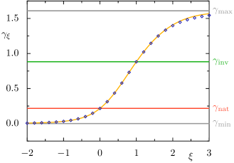
For $\xi=0$ just the first factor contributes in Eq. (16) and we recover $\mu_{\xi=0}=\mu_{\text{nat}}$. From Eq. (14) follows that $\gamma_{\xi=0}=\gamma_{\text{nat}}[R]=\gamma_{\text{nat}}$, where we used that $\gamma_{\text{inv}}[R^{0}]=0$. For $\xi=1$ we similarly have $\mu_{\xi=1}=\mu_{\text{inv}}$ and $\gamma_{\xi=1}=\gamma_{\text{inv}}$. Increasing $\xi$ from $0$ to $1$ a transition from $\mu_{\text{nat}}$ to $\mu_{\text{inv}}$ occurs. In Fig. 2 we show the dependence of the decay rate $\gamma_{\xi}$ on $\xi$, Eq. (14), for the example system. The decay rate $\gamma_{\xi}$ continuously increases with $\xi$ from $\gamma_{\text{min}}$ for $\xi\rightarrow-\infty$ to $\gamma_{\text{max}}$ for $\xi\rightarrow\infty$. Furthermore we determine $\gamma_{\xi}$ by iteration of the constructed measures $\mu_{\xi}$ using Eq. (5) with very good agreement with Eq. (14). The phase-space structure of $\mu_{\xi}$ is shown in Fig. 3(f-j), demonstrating the strong dependence on the decay rate and revealing the underlying hyperbolic structure. Note that for a closed map, i.e. without escape, $R(x)=1$, we obtain $\gamma_{\xi}=0$ and uniform distribution $\mu_{\xi}=\mu_{\text{L}}$ for all $\xi$.

IV Quantum-classical comparison

In this section we investigate to which extent the phase-space distributions of resonance eigenfunctions with decay rate $\gamma$ are described by the c-measures $\mu_{\xi}$ with $\gamma_{\xi}=\gamma$. This comparison is essential because for the same decay rate $\gamma$ there may be many different c-measures DemYou2006 ; NonRub2007 and it is not known which of the possible c-measures are quantum mechanically relevant in the case of partial escape. It is known that resonance eigenfunctions with decay rate $\gamma\approx\gamma_{\text{nat}}$ are well described by the natural measure $\mu_{\text{nat}}$ CasMasShe1999b , also in optical microcavities showing partial escape LeeRimRyuKwoChoKim2004 ; HarShi2015 ; KulWie2016 . Our first conjecture is that resonance eigenfunctions with decay rate $\gamma\approx\gamma_{\text{inv}}$ are well described by the inverse measure $\mu_{\text{inv}}$ in the semiclassical limit. This is motivated by using that the natural measure of the inverse map $\mathcal{M}^{-1}$ describes resonance eigenfunctions with $\gamma\approx\gamma_{\text{nat}}[\mathcal{M}^{-1}]$ of the inverse quantum map $\mathcal{U}^{-1}=\mathcal{R}^{-1}\tilde{\mathcal{U}}^{\dagger}$. These are the resonance eigenfunctions of $\mathcal{U}$ with decay rate $\gamma\approx\gamma_{\text{inv}}$. Our second conjecture is that resonance eigenfunctions with arbitrary decay rate $\gamma$ are well described by the c-measures $\mu_{\xi}$ with $\gamma_{\xi}=\gamma$.

The quantum-classical comparison is done by qualitatively comparing the phase-space distributions (Sec. IV.1), comparing the information dimension (Sec. IV.2), determining the Jensen-Shannon divergence (Sec. IV.3), studying the semiclassical limit (Sec. IV.4), and considering the limit of full escape (Sec. IV.5). We report numerical investigations for a representative example of fully chaotic system with partial absorption, the quantized standard map (see Appendix A). We find very good agreement for the natural measure $\mu_{\text{nat}}$ and the inverse measure $\mu_{\text{inv}}$ (first conjecture), and identify small deviations in the semiclassical limit for intermediate decay rates $\gamma_{\xi}$ (second conjecture).

IV.1 Phase-space distributions

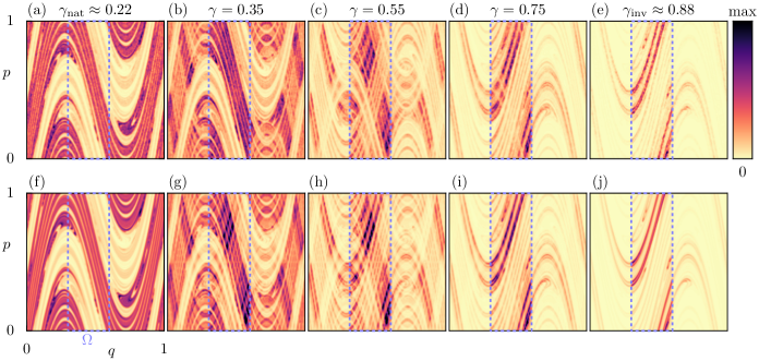
Figure Fig. 3 shows a remarkable similarity between the quantum Husimi distributions and the classical c-measures $\mu_{\xi}$ for different values of $\gamma$. The same multifractal structure and dramatic change with $\gamma$ are observed: For $\gamma\approx\gamma_{\text{nat}}$ the high-density filaments are concentrated along the unstable direction on the phase space and resemble the natural c-measure $\mu_{\text{nat}}$. For $\gamma\approx\gamma_{\text{inv}}$ the distribution concentrates along the stable direction with maximum inside the opening $\Omega$, resembling the inverse measure $\mu_{\text{inv}}$. For intermediate values of $\gamma$ the density concentrates on the product of the two previous structures, revealing the hyperbolic structure on phase space. Classically this behavior is understood from the definition of $\mu_{\xi}$, see Sec. III.3.

Note that the measures $\mu_{\xi}$ are illustrated on phase space by considering expectation values of Gaussian distributions $g_{x,\sigma}$, centered at $x\in\Gamma$ with width $\sigma=\sqrt{\hbar/2}$. This is the classical equivalent to the quantum expectation of an eigenfunction $\psi$ in a symmetric coherent state centered at $x\in\Gamma$. It is possible to choose asymmetric coherent states with different uncertainties in the phase-space variables $q$ and $p$ in the definition of the Husimi distribution. We find good qualitative agreement, if the classical expectation values are adapted accordingly (not shown).

The qualitative similarity of quantum and classical distributions confirms that the main features of the $\gamma$-dependence of resonance eigenfunctions has a classical origin. However, a closer inspection shows that there are small but still visible differences between the classical and quantum results (e.g. for $\gamma=0.55$ in the region $(q,p)\in[0.3,0.4]\times[0.3,0.6]$, see Fig. 3(c, h). This motivates us to pursue more quantitative comparisons between the measures, which will allow us to investigate their dependence on $\gamma$ and $h$.

Figure 4: Fractality of classical and quantum measures. The effective information dimension $D_{1}$ is shown as a function of the decay rate $\gamma$ for c-measures $\mu_{\xi}$ (blue diamonds) and for Husimi distributions $\mathcal{H}_{\gamma}$ at $h=1/16\,000$ (red stars). $D_{1}$ is computed from the scaling $S(\epsilon)\sim\log\epsilon^{-D_{1}}$ in the regime $\epsilon\in[1/4,1/16]$, see inset for the case $\gamma=\gamma_{\text{inv}}\approx 0.88$ ($D_{1}=2$ is expected for the quantum data in the regime $\epsilon\lesssim\sqrt{h}$, black dashed line). In the quantum case, $S(\epsilon)$ corresponds to the average entropy for eigenfunctions with decay rate in $(\gamma-\Delta\gamma,\gamma+\Delta\gamma)$ with $\Delta\gamma=0.016$ (equivalent results are obtained using the entropy of the average Husimi distribution). The shaded regions are confidence intervals estimated taking into account uncertainties in the linear regression and (for the quantum case) in the computation of average $S(\epsilon)$. Vertical dashed lines indicate $\gamma_{\text{nat}}$ and $\gamma_{\text{inv}}$. Standard map as in Fig. 1.

IV.2 Information dimension

In order to quantify the fractal properties of quantum and classical phase-space distributions we consider the information dimension $D_{1}$. It is defined for any measure $\mu$ as

$$D_{1}=\lim_{\epsilon\rightarrow 0}\frac{S(\epsilon;\mu)}{\log\epsilon^{-1}},$$ (17)

where the entropy $S(\epsilon;\mu)$ is defined for any normalized phase-space measure $\mu$ as

$$S(\epsilon;\mu)=-\sum_{A\in\mathcal{A}_{\epsilon}}p_{A}\log p_{A},$$ (18)

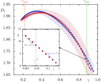
with $p_{A}\equiv\mu(A)=\int_{A}\text{d}\mu$ and $\mathcal{A}_{\epsilon}$ a partition of the phase-space in boxes $A$ of size $\mu_{\text{L}}(A)=\epsilon^{2}$. We choose $D_{1}$ instead of $D_{0}$ to quantify the fractality of the measures because $\mathcal{H}(x)>0$ almost everywhere on $\Gamma$ and therefore the box-counting dimension $D_{0}$ is equal to the phase space dimension AltPorTel2013b . For the Husimi distribution $\mathcal{H}$ the probability measure is defined as $\mu_{\mathcal{H}}(A)=\int_{A}\mathcal{H}\,\text{d}\mu_{\text{L}}$ (see Appendix C for details). As it is a smooth function on the scale of order $h$, any asymptotically ($\epsilon\rightarrow 0$) defined fractal dimension of $\mathcal{H}$ is trivial. Therefore, we focus on an effective fractal dimension $D_{1}$ in a regime $1>\epsilon\gtrsim\sqrt{h}$. The dimension $D_{1}$ (and entropies $S$) for resonance eigenfunctions with the same decay rate $\gamma$ should converge in the limit $h\rightarrow 0$ for a fixed value of $\epsilon$.

Figure 4 shows numerical results for $D_{1}$ of the quantum and classical measures. The inset confirms that $S$ shows a non-trivial scaling with $\epsilon$, defining an effective fractal dimension for the quantum (red stars) and classical (blue diamonds) distributions. The dependence of $D_{1}$ on the decay rate $\gamma$ shows an initial increase to a maximum value, followed by a decrease towards $D_{1}(\gamma_{\text{inv}})<D_{1}(\gamma_{\text{nat}})$. This shows that different fractal properties exist for different decay rates $\gamma$. Most importantly, the quantum and classical results show the same overall dependence. The distance between the values for $\mu_{\xi}$ and $\mathcal{H}_{\gamma}$ are smaller than the numerically estimated errors from the calculation of $D_{1}$. Therefore the fractal dimension of the c-measures $\mu_{\xi}$ can be used to estimate the fractal dimension of resonance eigenfunctions.

Figure 5: Comparison between the quantum measure and different classical measures as a function of the decay rate $\gamma$. The symbols correspond to the Jensen-Shannon divergence $d_{\text{JS}}$ between individual Husimi distributions $\mathcal{H}_{\gamma}$ and different classical measures $\mu_{\xi}$ (blue diamonds), $\mu_{\text{nat}}$ (red boxes), $\mu_{\text{inv}}$ (green triangles), and $\mu_{\text{L}}$ (gray circles). (a) $h=1/4\,000$ and (b) $h=1/16\,000$. Dotted lines indicate $\gamma_{\text{nat}}$ and $\gamma_{\text{inv}}$. The reported distances $d_{\text{JS}}$ were obtained with $\epsilon=1/16>\sqrt{h}$. Standard map as in Fig. 1.

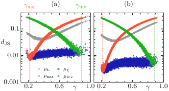
IV.3 Jensen-Shannon divergence

A quantification of the distance between the quantum and classical measures can be obtained using the Jensen-Shannon divergence GroBerCarRomOliSta2002 . For any two probability measures $\mu_{1}$ and $\mu_{2}$ it is given by the difference of the entropy of the sum of the distributions and the sum of the entropies of the single distributions,

$$d_{\text{JS}}(\epsilon;\mu_{1},\mu_{2})=S\left(\epsilon;\frac{\mu_{1}+\mu_{2}}{2}\right)-\frac{S(\epsilon;\mu_{1})+S(\epsilon;\mu_{2})}{2},$$ (19)

where $S$ is the entropy defined in Eq. (18). The square root of $d_{\text{JS}}$ is a distance and thus $d_{\text{JS}}(\mu_{1},\mu_{2})\geq 0$ with equality if and only if $\mu_{1}=\mu_{2}$. Again we need to introduce a scale of order $\epsilon$ defining the coarseness of the phase-space. For quantum-classical comparison the calculated difference is only meaningful if $\epsilon>\sqrt{h}$.

The Jensen-Shannon divergence between individual Husimi distributions and several classical measures is illustrated in Fig. 5(a) for different values of $\gamma$ and $h$. As expected, the distance to the natural measure $\mu_{\text{nat}}$ (red boxes) has a pronounced minimum at $\gamma=\gamma_{\text{nat}}$ and the distance to $\mu_{\text{inv}}$ at $\gamma_{\text{inv}}$ (green triangles). The distance to the uniform measure $\mu_{\text{L}}$ (gray circles) is larger than these minima, showing a minimum at around $\gamma\approx 0.4$ (related to the maximum of $D_{1}$ seen in Fig. 4, where $\mathcal{H}_{\gamma}$ is closer to uniformity). The distance to the c-measures $\mu_{\xi}$ (blue diamonds) shows much smaller values of $d_{\text{JS}}$ than for the other measures. There is almost no dependence on $\gamma$. Reducing $h$ in Fig. 5(b), we see that the quantum-classical distance reduces significantly for all $\gamma$. Variation of $\epsilon>\sqrt{h}$ gives similar results (with overall smaller distances for larger $\epsilon$ and vice versa).

Figure 6: Quantum-classical comparison in the semiclassical limit. The Jensen-Shannon divergence $d_{\text{JS}}$ between quantum distributions and the classical measure $\mu_{\xi}$ is shown as a function of $h$ for $\gamma\in\{\gamma_{\text{nat}}\approx 0.22,0.35,0.55,0.75,\gamma_{\text{inv}}\approx 0.88\}$. (a) Husimi distribution of individual resonances $\mathcal{H}_{\gamma}$, averaged over $\Delta\gamma=0.004$. Gray dashed line indicates numerical scaling for $\gamma_{\text{nat}}$. (b) Averaged Husimi distributions $\langle\mathcal{H}\rangle_{\gamma}$ with $\Delta\gamma=0.004$. Standard map as in Fig. 1.

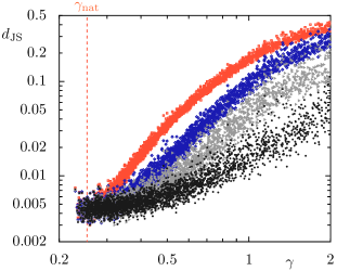
IV.4 Semiclassical limit

We focus on the quantum-classical comparison with the aim of testing whether our results are compatible with a distance $d_{\text{JS}}\rightarrow 0$ in the semiclassical limit, $h\rightarrow 0$. Distances $\langle d_{\text{JS}}(\mathcal{H}_{\gamma},\mu_{\xi})\rangle$ for a fixed scale $\epsilon=1/16\gg\sqrt{h}$ and five different decay rates $\gamma$ are shown in Fig. 6(a), comparing individual Husimi distributions $\mathcal{H}_{\gamma}$ and the classical measures $\mu_{\xi}$, averaged over $\Delta\gamma=0.004$. We observe a power-law $d_{\text{JS}}\sim h^{\delta}$ decay with $\delta\approx 0.77$. Distances of the same order and scaling are found when comparing individual Husimi distributions $\mathcal{H}_{\gamma}$ to the averaged Husimi distributions $\langle\mathcal{H}\rangle_{\gamma}$ (not shown). Therefore at these values of $h$ the distance and its decay is dominated by fluctuations around the average. Establishing a possible relationship between $\delta$ and fractal properties of $\mu_{\xi}$ remains an open question.

In order to obtain a more sensitive test we reduce the quantum fluctuations by computing averaged Husimi distributions $\langle\mathcal{H}\rangle_{\gamma}$ using eigenfunctions in an interval around $\gamma$. The results presented in Fig. 6(b) show therefore much smaller distances $d_{\text{JS}}$. For $\gamma_{\text{nat}}$ and $\gamma_{\text{inv}}$ we again find a power-law (with larger exponent), indicating semiclassical convergence. This gives strong evidence for our conjecture about the inverse measure $\mu_{\text{inv}}$. It also verifies the expectation CasMasShe1999b ; LeeRimRyuKwoChoKim2004 for the natural measure $\mu_{\text{nat}}$ on a quantitative level.

For intermediate values of $\gamma$, however, we observe a much slower decay of $d_{\text{JS}}$ with $h$. This suggests a saturation towards a finite distance $d_{\text{JS}}(\langle\mathcal{H}\rangle_{\gamma}^{h\rightarrow 0},\mu_{\xi})>0$. Thus the c-measures $\mu_{\xi}$ are not the semiclassical limit measures of the resonance eigenfunctions. We expect a similar saturation also for the individual Husimi distributions, as used in Fig. 6(a). However, this is expected for smaller values of the distance $d_{\text{JS}}$ (when it is no longer dominated by quantum fluctuations but by the distance of the classical measure to the average Husimi distribution) which occur for values of $h$ beyond the reach of current computational feasibility.

IV.5 Limit of full escape

Finally we investigate the dependence on the reflectivity $R_{\Omega}$. Our construction of $\mu_{\xi}$ can be performed for any system with partial escape ($R_{\Omega}\neq 0$) and our results hold, with quantitative changes due to the change in the fractality of the c-measures. For instance, in the limit of a closed system, $R_{\Omega}\rightarrow 1$, all $\mu_{\xi}$ approach the uniform (Liouville) measure. The most interesting case is the limit of full escape, i.e. when the reflectivity function only takes values $0$ or $1$. In our example system this corresponds to $R_{\Omega}=0$ in the opening and $R=1$ in the remaining part of phase space. Classically, regions of full and partial escape are typically treated differently, e.g., in the operator proposed in Ref. AltPorTel2013b . Most importantly, when regions of full escape exist, the open map $\mathcal{M}$ is not invertible, so that $\mu_{\text{inv}}$ is not well-defined and the measures $\mu_{\xi}$ cannot be constructed directly. In order to investigate how $\mu_{\xi}$ behaves in the case of full escape, here we consider the limit $\mu_{\xi}[R_{\Omega}\rightarrow 0]$. It is important in this limit to adjust the parameter $\xi$ such that the decay rate $\gamma$ remains fixed. In this way we obtain a c-measure with decay rate $\gamma$ for the system with full escape.

In Fig. 7 we show the Jensen-Shannon divergence $d_{\text{JS}}$ comparing resonance eigenfunctions of the system with full escape ($R_{\Omega}=0$) to the measures $\mu_{\xi}[R_{\Omega}=10^{-4}]$ (blue diamonds). We verified that results do not change for smaller $R_{\Omega}$. While we find good agreement for decay rates close to $\gamma_{\text{nat}}$, the distance grows drastically with $\gamma$. Even though the distance is smaller than for $\mu_{\text{nat}}$ (red squares), the measures $\mu_{\xi}$ clearly do not correspond to resonance eigenfunctions in this limit. This discrepancy is not surprising, since the $\gamma$-dependence of $\mu_{\xi}$ is partly based on information about forward iterations of phase-space points, which is completely lost when falling into the opening with $R_{\Omega}=0$.

Much smaller distances are obtained using the c-measures proposed for systems with full escape in Ref. ClaKoeBaeKet2018 (black circles). Their construction is based on a uniform distribution on subsets with the same temporal distance to the chaotic saddle, which is the invariant set of the system with full escape. Using the Jensen-Shannon divergence we are able to quantify their agreement to resonance eigenfunctions. We observe that the distance grows with $\gamma$, seen already qualitatively in Ref. ClaKoeBaeKet2018 . Note that the quantitative analysis confirms that these measures are in better agreement than the c-measures of Ref. KoeBaeKet2015 (light gray triangles). Note also that for $\gamma=\gamma_{\text{nat}}$ all considered measures are identical explaining why they have the same distance $d_{\text{JS}}$.

Figure 7: Quantum-classical comparison for systems with full escape. The Jensen-Shannon divergence $d_{\text{JS}}(\epsilon=1/16)$ is shown as a function of $\gamma$ for fixed $h=1/16\,000$. The Husimi distribution $\mathcal{H}_{\gamma}$ of individual eigenfunctions is compared to different classical measures: $\mu_{\text{nat}}$ (red squares), $\mu_{\xi}$ for small $R_{\Omega}=10^{-4}$ (blue diamonds), c-measures of Ref. ClaKoeBaeKet2018 (black circles), and c-measures of Ref. KoeBaeKet2015 (gray triangles). Standard map as in Fig. 1, but with $R_{\Omega}=0$. The dashed line indicates $\gamma_{\text{nat}}\approx 0.25$ for this case.

V Conclusions

In summary, we construct a one-parameter family of classical conditionally invariant measures (c-measures) $\mu_{\xi}$ that explains the main properties of quantum resonance eigenfunctions in systems with partial escape. We confirm previous observations that the natural c-measure $\mu_{\text{nat}}=\mu_{\xi=0}$ describes long-lived eigenfunctions with decay rate $\gamma=\gamma_{\text{nat}}$ in the semiclassical limit $h\to 0$, including numerical tests of this correspondence with unprecedented precision. We find a similar good numerical agreement between the natural c-measure of the inverse system $\mu_{\text{inv}}=\mu_{\xi=1}$ and short-lived eigenfunctions with $\gamma=\gamma_{\text{inv}}$, supporting our conjecture about the inverse measure.

The importance of our results is that they apply to arbitrary decay rates $\gamma$. We numerically observe that the decay rates of almost all resonances lie in the interval $\gamma_{\text{nat}}\leq\gamma\leq\gamma_{\text{inv}}$. Our construction of $\mu_{\xi}$, Eq. (16), is based on the product structure in hyperbolic systems and combines $\mu_{\text{nat}}$ and $\mu_{\text{inv}}$. It leads to measures in the complete range of classical decay rates, i.e., $\gamma_{\xi\to-\infty}=\gamma_{\text{min}}$ and $\gamma_{\xi\to\infty}=\gamma_{\text{max}}$, being thus applicable to describe all possible resonances. Numerical simulations in the standard map show that $\mu_{\xi}$ captures the main features of the quantum resonance eigenfunctions with $\gamma=\gamma_{\xi}$: They show compatible fractal dimensions and the same drastic dependence of the phase-space structure on the decay rate $\gamma$ changing from unstable to stable direction. The semiclassical behavior $h\rightarrow 0$ gives strong evidence that for $\gamma_{\text{nat}}$ and $\gamma_{\text{inv}}$ the corresponding measures $\mu_{\text{nat}}$ and $\mu_{\text{inv}}$ are the semiclassical limits of resonance eigenfunctions, while for intermediate rates we find no convergence. We also find that in the limit of full escape the measures $\mu_{\xi}$ do not describe resonance eigenfunctions as good as previous approaches. Altogether, our numerical results suggest that $\mu_{\xi}$ is not the semiclassical limit measure, unless $\xi=0$ or $\xi=1$. Possible improvements could consider alternative combinations of $\mu_{\text{nat}}$ and $\mu_{\text{inv}}$ or incorporate local Ehrenfest times instead of the fixed iteration number in Eq. (16).

Finally, it is straightforward to generalize the construction of measures $\mu_{\xi}$ to true time maps AltPorTel2013b ; AltPorTel2015 . This would allow for a description of resonance eigenfunctions in billiards with partial escape and thus in models of optical microcavities. There the structure of resonance eigenfunctions has observable consequences in the far-field emission of these cavities.

VI Appendix

Appendix A Example: Standard map

A.1 Classical

In order to investigate the inverse measure $\mu_{\text{inv}}$ and the intermediate measures $\mu_{\xi}$ numerically, we consider the paradigmatic standard map Chi1979 . It is given by the time-periodically driven Hamiltonian $H(q,p)=p^{2}/2+\sum_{n}V(q)\delta(t-n)$, with dimensionless coordinates $x\equiv(q,p)$ on phase-space $\Gamma=[0,1)\times[0,1)$ and kicking potential $V(q)=\kappa/(4\pi^{2})\cos(2\pi q)$. We consider the half-kick mapping, which takes the form $M(q,p)=(q+p^{\ast},p^{\ast}-V^{\prime}(q+p^{\ast})/2)$ with $p^{\ast}=p-V^{\prime}(q)/2$. All numerical results are computed for $\kappa=10$, for which the phase space is chaotic with no visible regular regions. Escape is introduced by considering a phase-space region $\Omega$ (a leak) such that the reflectivity $R(x)=R_{\Omega}<1$ for $x\in\Omega$ and $R(x)=1$ for $x\notin\Omega$. This mimics the behavior of more realistic couplings (e.g., Fresnel’s law in optical microresonators). Numerical results are presented for a strip in $p$-direction on the phase-space, $\Omega=(0.3,0.6)\times[0,1)$, with $R_{\Omega}=0.2$.

For the classical investigation we compute numerical approximations of the measures $\mu_{\xi}$. First, we fix the number $n$ of time-steps for the approximation $\tilde{\mu}_{\xi}^{n}$, see Eq. (16). Secondly, we fix a set $X_{c}$ of $\sqrt{N_{c}}\times\sqrt{N_{c}}$ phase-space points on a grid. The minimal distance $1/\sqrt{N_{c}}$ between two points defines the classical resolution and should be much smaller than $\sqrt{h}$. Note that for fixed $n$ and increasing $N_{c}$ we get better approximations of $\tilde{\mu}_{\xi}^{n}$. For each grid point $x\in X_{c}$ we compute the orbit $\{M^{k}(x)\}_{k=-n}^{n-1}$. which is used in Eq. (16). There the integral $\tilde{\mu}_{\xi}^{n}(A)$ is given by the sum of all contributions of points $x\in X_{c}\cap A$. Finally we consider the approximate measure $\mu_{\xi}^{n}\equiv\frac{\tilde{\mu}_{\xi}^{n}}{\|\tilde{\mu}_{\xi}^{n}\|}$.

Figure 8: Jensen-Shannon divergence $d_{\text{JS}}(\epsilon=1/16)$ for estimating convergence, conditional invariance, and accuracy of classical construction for fixed number of initial conditions $N_{c}=8192^{2}$. (a) Considered is $d_{\text{JS}}$ between $\mu_{\xi}^{n}$ and its normalized iterate $\mathcal{M}\mu_{\xi}^{n}/\|\mathcal{M}\mu_{\xi}^{n}\|$ over number of time-steps $n$ for $\xi\in\{0,0.3,0.5,0.7,1\}$. (b) Distance $d_{\text{JS}}(\mu_{\xi}^{n},\mu_{\xi}^{n+1})$ between numerical constructions with increasing number of time-steps $n$ plotted over number of time-steps $n$ for same $\xi$ as in (a). (c) Average Jensen-Shannon divergence $d_{\text{JS}}(\mu_{\xi}^{n},\hat{\mu}_{\xi}^{n})$ and standard deviation between $\mu_{\xi}^{n}$ and $10$ different realizations of $\hat{\mu}^{n}_{\xi}$ with random-uniform initial points on $\Gamma$ for fixed $n=8$.

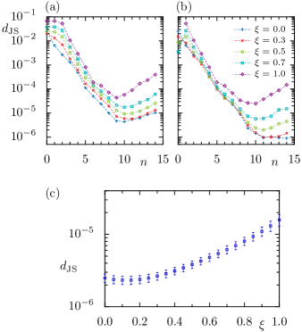
In the following we report properties of the classical measures regarding their conditional invariance, their convergence with $n$, and the accuracy of the classical construction used in this paper. This is illustrated in Fig. 8 for $N_{c}=8192^{2}$ initial phase-space points. Conditional invariance is investigated with the Jensen-Shannon divergence $d_{\text{JS}}$ between approximation $\mu_{\xi}^{n}$ and its normalized iterate $\mathcal{M}\mu_{\xi}^{n}/\|\mathcal{M}\mu_{\xi}^{n}\|$, see Fig. 8(a). Increasing values of $n$ lead to a decreasing $d_{\text{JS}}$ for all considered values of $\xi\in\{0,0.3,0.5,0.7,1\}$, up to a maximal number $\tilde{n}$. Thus $\mu_{\xi}^{n}$ fulfills condition (5) with increasing $n$. The limiting step $\tilde{n}$ is explained by the finite phase-space resolution given by the fixed number of points $N_{c}$.

Secondly, we numerically show that $d_{\text{JS}}(\mu_{\xi}^{n},\mu_{\xi}^{n+1})$ decreases with $n$ for all considered $\xi$, see Fig. 8(b). Thus it indicates weak convergence of $\mu_{\xi}^{n}$. The same restrictions due to the finite number of points $N_{c}$ apply here. Based on these results we use $\mu_{\xi}^{n}$ with $n=8$ as an approximation for $\mu_{\xi}$ throughout the paper. For these parameters we numerically obtain decay rates $\gamma_{\text{nat}}\approx 0.2165$ and $\gamma_{\text{inv}}\approx 0.8820$.

Moreover, we calculate the Jensen-Shannon divergence $d_{\text{JS}}$ between two different numerical approximations $\mu_{\xi}^{n}$ (defined above with $N_{c}$ grid-points) and $\hat{\mu}^{n}_{\xi}$ with $N_{c}$ random-uniform initial conditions. This is needed to ensure that the distance between quantum and classical measures is not influenced by classical fluctuations due to the numerical construction. We fix the number of time-steps $n=8$. We estimate the classical error as the difference between $\mu_{\xi}^{n}$ and $\hat{\mu}^{n}_{\xi}$ for different realizations of $\hat{\mu}^{n}_{\xi}$. The results are given in Fig. 8(c). Here we show the average of the distances $d_{\text{JS}}(\mu_{\xi}^{n},\hat{\mu}^{n}_{\xi})$ vs. $\xi$ and their standard-deviation for $10$ realizations. This gives an estimate on the accuracy of the constructed and considered measures $\mu_{\xi}^{n}$. We observe that for $\xi=0$ ($\gamma_{\text{nat}}$) the accuracy is nearly one magnitude smaller than for $\xi=1$ ($\gamma_{\text{inv}}$), and that the dependence is continuous. In all cases the errors are much smaller than the quantum-classical distances investigated in Sec. IV.3.

A.2 Quantum

The unitary quantum time-evolution in between two kicks is determined by Floquet quantization BerBalTabVor1979 ; ChaShi1986 . For the half-kick mapping it reads

$$\tilde{\mathcal{U}}=\text{e}^{-\frac{\text{i}}{2\hbar}V(\hat{q})}\text{e}^{-\frac{\text{i}}{2\hbar}\hat{p}^{2}}\text{e}^{-\frac{\text{i}}{2\hbar}V(\hat{q})},$$ (20)

where $h=2\pi\hbar$ takes the role of an effective Planck’s constant due to dimensionless units $q$ and $p$. Considering periodic boundary conditions, i.e. dynamics on a torus, only discrete values $h=1/N$ with $N\in\mathbb{N}$ are allowed. The semiclassical limit is described by the limit $h\rightarrow 0$. Due to the simple form of the reflectivity $R(x)$ the projective coupling operator NonSch2008 takes the form

$$\mathcal{R}=\mathcal{P}_{\Omega^{\text{c}}}+\sqrt{R_{\Omega}}\mathcal{P}_{\Omega}.$$ (21)

Note, that the second term $\sqrt{R_{\Omega}}\mathcal{P}_{\Omega}$ reduces the probability on $\Omega$ by a factor of $R_{\Omega}$. For $R_{\Omega}<1$ we obtain a subunitary time-evolution operator $\mathcal{U}=\tilde{\mathcal{U}}\mathcal{R}$ for the system with escape. Therefore all eigenvalues $\lambda=\text{e}^{\text{i}\theta-\gamma/2}$ have modulus less than one, i.e. decay rates $\gamma>0$.

We investigate the resonance eigenfunctions $\psi$ of $\mathcal{U}$ with decay rate $\gamma$ through their Husimi phase-space distribution $\mathcal{H}(x)$ Hus1940 , which is a smooth function. It is defined as the expectation value of the state $\psi$ in a coherent state $|x\rangle$ centered at $x\in\Gamma$, $\mathcal{H}_{\psi}(x)=h^{-1}|\langle x|\psi\rangle|^{2}$. For a single eigenfunction $\psi$ this distribution shows strong quantum fluctuations, illustrated in Fig. 1(d-f). A much clearer phase-space representation is obtained by considering the average $\langle\mathcal{H}\rangle_{\gamma}$ over all $\mathcal{H}_{\psi}$ where the decay rate of $\psi$ is in the interval $(\gamma-\Delta\gamma,\gamma+\Delta\gamma)$.

Appendix B Conditional invariance of $\mu_{\xi}$

Here we argue that $\mu_{\xi}$ is a c-measure, $\mathcal{M}\mu_{\xi}=\text{e}^{-\gamma_{\xi}}\mu_{\xi}$, Eq. (5), if the considered closed map $M$ is uniformly hyperbolic. Note that this condition is rather restrictive and is not satisfied by the standard map. The main idea is to use the local decomposition into stable and unstable direction and thereby splitting the two-dimensional integrals into two separate one-dimensional integrals. For the natural measure we obtain that it is continuous in the stable direction, while it is fractal along the unstable direction. Locally we can write $\mu_{\text{nat}}(A)=\mu_{\text{nat}}^{u}(A_{1})\otimes\mu_{\text{c}}^{s}(A_{2})$, where $\mu_{\text{nat}}^{u}$ and $\mu_{c}^{s}$ are fractal and continuous measures on $\mathbb{R}$, respectively. Note that this includes a local coordinate transformation from the phase space to the tangent space, including the Jacobian determinant in the integrals. Time evolution $\mathcal{M}$ gives an additional factor $R$, see Eq. (4), which together with $\mu_{\text{nat}}^{u}$ in the unstable direction leads to the decay $\text{e}^{-\gamma_{\text{nat}}}$. On the other hand, for the inverse measure, we obtain fractality along the stable direction only. Similarly we can locally write $\mu_{\text{inv}}(A)=\mu_{\text{c}}^{u}(A_{1})\otimes\mu_{\text{inv}}^{s}(A_{2})$ with continuous $\mu_{\text{c}}^{u}$ and fractal $\mu_{\text{inv}}^{s}$ measures on $\mathbb{R}$. Application of $\mathcal{M}$ gives the factor $R$, which together with $\mu_{\text{inv}}^{s}$ in the stable direction leads to the global decay $\text{e}^{-\gamma_{\text{inv}}}$.

In this sense, the measures for intermediate decay rates $\mu_{\xi}$ can locally be understood as $\mu_{\xi}=\mu_{\text{nat}}^{u}[R^{1-\xi}]\otimes\mu_{\text{inv}}^{s}[R^{\xi}]$, where $\mu_{\text{nat}}^{u}[R^{1-\xi}]$ is the natural measure obtained for the map with escape $R^{1-\xi}$ and $\mu_{\text{inv}}^{s}[R^{\xi}]$ is the inverse measure obtained for the map with escape $R^{\xi}$. The additional factor $R$ from time-evolution, Eq. (4), can be split into $R^{1-\xi}$ and $R^{\xi}$. The first leads to the decay rate $\gamma_{\text{nat}}[R^{1-\xi}]$ corresponding to $\mu_{\text{nat}}^{u}[R^{1-\xi}]$, while the second gives $\gamma_{\text{inv}}[R^{\xi}]$ corresponding to $\mu_{\text{inv}}^{s}[R^{\xi}]$. Thus the decay rate of the measures $\mu_{\xi}$ is given by Eq. (14), $\gamma_{\xi}=\gamma_{\text{nat}}[R^{1-\xi}]+\gamma_{\text{inv}}[R^{\xi}]$.

Appendix C Entropy of Husimi distributions

We want to define the entropy of Husimi distributions of eigenfunctions with decay rate $\gamma$. Defining the probability measure $\mu_{\mathcal{H}}(A)=\int_{A}\mathcal{H}\,\text{d}\mu_{\text{L}}$ for each $\gamma$ we obtain the entropies $S(\epsilon;\mu_{\mathcal{H}})$, Eq. (18). Because we are interested in the dependence on $\epsilon$, we reduce fluctuations by considering the average entropy of eigenfunctions with decay rate in the interval $(\gamma-\Delta\gamma,\gamma+\Delta\gamma)$. This is given for fixed $\epsilon$ by

$$\langle S_{\epsilon}\rangle_{\gamma} =\frac{1}{n_{\gamma}}\sum\limits_{|\gamma-\tilde{\gamma}|<\Delta\gamma}S(\epsilon;\mu_{\mathcal{H}})$$ (22)

$$=-\sum\limits_{A\in\mathcal{A}}\ \frac{1}{n_{\gamma}}\sum\limits_{|\gamma-\tilde{\gamma}|<\Delta\gamma}p_{\tilde{\gamma},A}\log p_{\tilde{\gamma},A},$$ (23)

with number of eigenfunctions in the interval $n_{\gamma}={\#\{|\gamma-\tilde{\gamma}|<\Delta\gamma\}}$ and $p_{\tilde{\gamma},A}=\int_{A}\mathcal{H}_{\gamma}\,\text{d}\mu_{\text{L}}$. Fixing $\epsilon$ it is possible to define an effective semiclassical limit as $S_{q}(\epsilon;\gamma)\equiv\lim_{h\rightarrow 0}\langle S_{\epsilon}\rangle_{\gamma}$ with fixed decay rate $\gamma$ and decreasing $h$. The scaling of $S_{q}$ with $\epsilon$ eventually defines the fractal dimension $D_{1}$ of the quantum limit. Numerically we have to deal with finite values of $h$ and effective entropies at this value. We determine the fractal dimension $D_{1}$ of the quantum eigenfunctions with decay rate $\gamma$ from the scaling of $\langle S\rangle_{\gamma}$ with $\epsilon$. Note that in this case Planck’s scale $h$ defines a minimal resolution for $\epsilon$ below which there is no fractality and the trivial result $D_{1}=2$ is recovered.

References

- (1) O. Bohigas, M. J. Giannoni, and C. Schmit: “Characterization of chaotic quantum spectra and universality of level fluctuation laws”, Phys. Rev. Lett. 52, 1–4 (1984).
- (2) M. V. Berry: “Semiclassical theory of spectral rigidity”, Proc. R. Soc. Lon. A 400, 229–251 (1985).
- (3) M. Sieber and K. Richter: “Correlations between periodic orbits and their rôle in spectral statistics”, Phys. Scripta 2001, 128–133 (2001).
- (4) S. Müller, S. Heusler, P. Braun, F. Haake, and A. Altland: “Semiclassical foundation of universality in quantum chaos”, Phys. Rev. Lett. 93, 014103 (2004).
- (5) A. Voros: “Semi-classical ergodicity of quantum eigenstates in the Wigner representation”, in G. Casati and J. Ford (editors) “Stochastic Behavior in Classical and Quantum Hamiltonian Systems”, volume 93 of Lecture Notes in Physics, 326–333, Springer Berlin Heidelberg, Berlin (1979).
- (6) M. V. Berry: “Regular and irregular semiclassical wavefunctions”, J. Phys. A 10, 2083–2091 (1977).
- (7) M. V. Berry: “Semiclassical mechanics of regular and irregular motion”, in G. Iooss, R. H. G. Helleman, and R. Stora (editors) “Comportement Chaotique des Systèmes Déterministes — Chaotic Behaviour of Deterministic Systems”, 171–271, North-Holland, Amsterdam (1983).
- (8) A. I. Shnirelman: “Ergodic properties of eigenfunctions (in Russian)”, Usp. Math. Nauk 29, 181–182 (1974).
- (9) Y. Colin de Verdière: “Ergodicité et fonctions propres du laplacien (in French)”, Commun. Math. Phys. 102, 497–502 (1985).
- (10) S. Zelditch: “Uniform distribution of eigenfunctions on compact hyperbolic surfaces”, Duke. Math. J. 55, 919–941 (1987).
- (11) S. Zelditch and M. Zworski: “Ergodicity of eigenfunctions for ergodic billiards”, Commun. Math. Phys. 175, 673–682 (1996).
- (12) S. Nonnenmacher and A. Voros: “Chaotic eigenfunctions in phase space”, J. Stat. Phys. 92, 431–518 (1998).
- (13) A. Bäcker, R. Schubert, and P. Stifter: “Rate of quantum ergodicity in Euclidean billiards”, Phys. Rev. E 57, 5425–5447 (1998), ; erratum ibid. 58 (1998) 5192.
- (14) S. De Bièvre: “Quantum chaos: a brief first visit”, in S. Pérez-Esteva and C. Villegas-Blas (editors) “Second Summer School in Analysis and Mathematical Physics (Cuernavaca, 2000)”, Contemp. Math. 289, 161–218, Amer. Math. Soc., Providence, RI (2001).
- (15) H. Cao and J. Wiersig: “Dielectric microcavities: Model systems for wave chaos and non-Hermitian physics”, Rev. Mod. Phys. 87, 61–111 (2015).
- (16) G. E. Mitchell, A. Richter, and H. A. Weidenmüller: “Random matrices and chaos in nuclear physics: Nuclear reactions”, Rev. Mod. Phys. 82, 2845–2901 (2010).
- (17) H.-J. Stöckmann: Quantum Chaos: An Introduction, Cambridge University Press, Cambridge (1999).
- (18) Y.-C. Lai and T. Tél: Transient Chaos: Complex Dynamics on Finite Time Scales, number 173 in Applied Mathematical Sciences, Springer Verlag, New York, 1 edition (2011).
- (19) E. G. Altmann, J. S. E. Portela, and T. Tél: “Leaking chaotic systems”, Rev. Mod. Phys. 85, 869–918 (2013).
- (20) P. Gaspard: “Quantum chaotic scattering”, Scholarpedia 9(6), 9806 (2014).
- (21) G. Casati, G. Maspero, and D. L. Shepelyansky: “Quantum fractal eigenstates”, Physica D 131, 311–316 (1999).
- (22) J. P. Keating, M. Novaes, S. D. Prado, and M. Sieber: “Semiclassical structure of chaotic resonance eigenfunctions”, Phys. Rev. Lett. 97, 150406 (2006).
- (23) S. Nonnenmacher and M. Rubin: “Resonant eigenstates for a quantized chaotic system”, Nonlinearity 20, 1387–1420 (2007).
- (24) F. Borgonovi, I. Guarneri, and D. L. Shepelyansky: “Statistics of quantum lifetimes in a classically chaotic system”, Phys. Rev. A 43, 4517–4520 (1991).
- (25) H. Schomerus and J. Tworzydło: “Quantum-to-classical crossover of quasibound states in open quantum systems”, Phys. Rev. Lett. 93, 154102 (2004).
- (26) J. P. Keating, S. Nonnenmacher, M. Novaes, and M. Sieber: “On the resonance eigenstates of an open quantum baker map”, Nonlinearity 21, 2591–2624 (2008).
- (27) L. Ermann, G. G. Carlo, and M. Saraceno: “Localization of resonance eigenfunctions on quantum repellers”, Phys. Rev. Lett. 103, 054102 (2009).
- (28) K. Clauß, M. J. Körber, A. Bäcker, and R. Ketzmerick: “Resonance eigenfunction hypothesis for chaotic systems”, Phys. Rev. Lett. 121, 074101 (2018).
- (29) A. M. Bilen, I. García-Mata, B. Georgeot, and O. Giraud: “Multifractality of open quantum systems”, Phys. Rev. E 100, 032223 (2019).
- (30) P. Gaspard and S. A. Rice: “Scattering from a classically chaotic repellor”, J. Chem. Phys. 90, 2225–2241 (1989).
- (31) G. Pianigiani and J. A. Yorke: “Expanding maps on sets which are almost invariant: Decay and chaos”, Trans. Amer. Math. Soc. 252, 351–366 (1979).
- (32) M. F. Demers and L.-S. Young: “Escape rates and conditionally invariant measures”, Nonlinearity 19, 377–397 (2006).
- (33) J. Sjöstrand: “Geometric bounds on the density of resonances for semiclassical problems”, Duke Math. J. 60, 1–57 (1990).
- (34) K. K. Lin: “Numerical study of quantum resonances in chaotic scattering”, J. Comput. Phys. 176, 295–329 (2002).
- (35) W. T. Lu, S. Sridhar, and M. Zworski: “Fractal Weyl laws for chaotic open systems”, Phys. Rev. Lett. 91, 154101 (2003).
- (36) J. A. Ramilowski, S. D. Prado, F. Borondo, and D. Farrelly: “Fractal Weyl law behavior in an open Hamiltonian system”, Phys. Rev. E 80, 055201(R) (2009).
- (37) A. Eberspächer, J. Main, and G. Wunner: “Fractal Weyl law for three-dimensional chaotic hard-sphere scattering systems”, Phys. Rev. E 82, 046201 (2010).
- (38) L. Ermann and D. L. Shepelyansky: “Ulam method and fractal Weyl law for Perron-Frobenius operators”, Eur. Phys. J. B 75, 299–304 (2010).
- (39) S. Nonnenmacher, J. Sjöstrand, and M. Zworski: “Fractal Weyl law for open quantum chaotic maps”, Annals of Mathematics 179, 179–251 (2014).
- (40) S.-Y. Lee, S. Rim, J.-W. Ryu, T.-Y. Kwon, M. Choi, and C.-M. Kim: “Quasiscarred resonances in a spiral-shaped microcavity”, Phys. Rev. Lett. 93, 164102 (2004).
- (41) J. Wiersig and M. Hentschel: “Combining directional light output and ultralow loss in deformed microdisks”, Phys. Rev. Lett. 100, 033901 (2008).
- (42) J. Wiersig and J. Main: “Fractal Weyl law for chaotic microcavities: Fresnel’s laws imply multifractal scattering”, Phys. Rev. E 77, 036205 (2008).
- (43) J.-B. Shim, J. Wiersig, and H. Cao: “Whispering gallery modes formed by partial barriers in ultrasmall deformed microdisks”, Phys. Rev. E 84, 035202(R) (2011).
- (44) S. Shinohara, T. Harayama, T. Fukushima, M. Hentschel, T. Sasaki, and E. E. Narimanov: “Chaos-assisted directional light emission from microcavity lasers”, Phys. Rev. Lett. 104, 163902 (2010).
- (45) E. G. Altmann, J. S. E. Portela, and T. Tél: “Chaotic systems with absorption”, Phys. Rev. Lett. 111, 144101 (2013).
- (46) T. Harayama and S. Shinohara: “Ray-wave correspondence in chaotic dielectric billiards”, Phys. Rev. E 92, 042916 (2015).
- (47) E. G. Altmann, J. S. E. Portela, and T. Tél: “Chaotic explosions”, EPL 109, 30003 (2015).
- (48) J. Kullig and J. Wiersig: “Frobenius–Perron eigenstates in deformed microdisk cavities: non-Hermitian physics and asymmetric backscattering in ray dynamics”, New J. Phys. 18, 015005 (2016).
- (49) S. Nonnenmacher and E. Schenck: “Resonance distribution in open quantum chaotic systems”, Phys. Rev. E 78, 045202(R) (2008).
- (50) A. Potzuweit, T. Weich, S. Barkhofen, U. Kuhl, H.-J. Stöckmann, and M. Zworski: “Weyl asymptotics: From closed to open systems”, Phys. Rev. E 86, 066205 (2012).
- (51) B. Gutkin and V. A. Osipov: “Universality in spectral statistics of open quantum graphs”, Phys. Rev. E 91, 060901(R) (2015).
- (52) M. Schönwetter and E. G. Altmann: “Quantum signatures of classical multifractal measures”, Phys. Rev. E 91, 012919 (2015).
- (53) M. J. Körber, M. Michler, A. Bäcker, and R. Ketzmerick: “Hierarchical fractal Weyl laws for chaotic resonance states in open mixed systems”, Phys. Rev. Lett. 111, 114102 (2013).
- (54) G. G. Carlo, R. M. Benito, and F. Borondo: “Theory of short periodic orbits for partially open quantum maps”, Phys. Rev. E 94, 012222 (2016).
- (55) C. A. Prado, G. G. Carlo, R. M. Benito, and F. Borondo: “Role of short periodic orbits in quantum maps with continuous openings”, Phys. Rev. E 97, 042211 (2018).
- (56) D. Lippolis, J.-W. Ryu, S.-Y. Lee, and S. W. Kim: “On-manifold localization in open quantum maps”, Phys. Rev. E 86, 066213 (2012).
- (57) D. Lippolis, J.-W. Ryu, and S. W. Kim: “Localization in chaotic systems with a single-channel opening”, Phys. Rev. E 92, 012921 (2015).
- (58) Y. V. Fyodorov and H.-J. Sommers: “Spectra of random contractions and scattering theory for discrete-time systems”, J. Exp. Theor. Phys. Lett. 72, 422–426 (2000).
- (59) J. P. Keating, M. Novaes, and H. Schomerus: “Model for chaotic dielectric microresonators”, Phys. Rev. A 77, 013834 (2008).
- (60) D. L. Shepelyansky: “Fractal Weyl law for quantum fractal eigenstates”, Phys. Rev. E 77, 015202(R) (2008).
- (61) K. Husimi: “Some formal properties of the density matrix”, Proc. Phys. Math. Soc. Jpn. 22, 264–314 (1940).
- (62) N. Chernov and R. Markarian: “Ergodic properties of Anosov maps with rectangular holes”, Bol. Soc. Bras. Mat 28, 271–314 (1997).
- (63) N. Chernov, R. Markarian, and S. Troubetzkoy: “Invariant measures for Anosov maps with small holes”, Ergodic Theory Dynam. Systems 20, 1007–1044 (2000).
- (64) S. M. Ulam: “A collection of mathematical problems”, in L. Bers, R. Courant, and J. J. Stoker (editors) “Interscience tracts in pure and applied Mathematics”, volume 8, 73–75, Interscience, New York (1960).
- (65) I. Grosse, P. Bernaola-Galván, P. Carpena, R. Román-Roldán, J. Oliver, and H. E. Stanley: “Analysis of symbolic sequences using the Jensen-Shannon divergence”, Phys. Rev. E 65, 041905 (2002).
- (66) M. J. Körber, A. Bäcker, and R. Ketzmerick: “Localization of chaotic resonance states due to a partial transport barrier”, Phys. Rev. Lett. 115, 254101 (2015).
- (67) B. V. Chirikov: “A universal instability of many-dimensional oscillator systems”, Phys. Rep. 52, 263–379 (1979).
- (68) M. V. Berry, N. L. Balazs, M. Tabor, and A. Voros: “Quantum maps”, Ann. Phys. (N.Y.) 122, 26–63 (1979).
- (69) S.-J. Chang and K.-J. Shi: “Evolution and exact eigenstates of a resonant quantum system”, Phys. Rev. A 34, 7–22 (1986).