Study of relativistic magnetized outflows with relativistic equation of state

Abstract

We study relativistic magnetized outflows using relativistic equation of state having variable adiabatic index ($\Gamma$) and composition parameter $(\xi)$. We study the outflow in special relativistic magneto-hydrodynamic regime, from sub-Alfvénic to super-fast domain. We showed that, after the solution crosses the fast point, magnetic field collimates the flow and may form a collimation-shock due to magnetic field pinching/squeezing. Such fast, collimated outflows may be considered as astrophysical jets. Depending on parameters, the terminal Lorentz factors of an electron-proton outflow can comfortably exceed few tens. We showed that due to the transfer of angular momentum from the field to the matter, the azimuthal velocity of the outflow may flip sign. We also study the effect of composition $(\xi)$ on such magnetized outflows. We showed that relativistic outflows are affected by the location of the Alfvén point, the polar angle at the Alfvén point and also the angle subtended by the field lines with the equatorial plane, but also on the composition of the flow. The pair dominated flow experiences impressive acceleration and is hotter than electron proton flow.

1 Introduction

There are many observational evidences that astrophysical objects like young stellar objects (YSOs), accreting white dwarfs, X-ray binaries (XRBs), and active galactic nuclei (AGN) produce jets. AGN jet is a relativistic, collimated outflow which spans over large distance (few kpc to Mpc scale) with Lorentz factor ($\gamma$) ranging from few to few tens. There are mainly three things which are common in astrophysical jets — first, jets are collimated (Asada & Nakamura, 2012), second, jets propagate with high speeds (Pearson et. al., 1981) and the third is the over-collimation of the flow due to interaction with the ambient medium and/or by the magnetic field pinching (Asada & Nakamura, 2012; Lii et. al., 2012). The bright knots observed throughout the jet, may occur due to the existence of multiple shocks caused by magnetic pinching, or, interaction with the ambient medium. There are many processes that can drive the jet outward with significant speed. In principle, thermal-pressure gradient term can accelerate the jet to speeds comparable to the sound speed at the jet base (Lee et. al., 2016). However, Meliani et. al. (2004) used the thermal-pressure gradient term as the main accelerating process, but achieved fast outflows by tweaking the equation of state of the flow. The intense radiation field emanating from the associated accretion disc, may transfer momentum or energy to the jet material and thereby accelerate it (see, Ferrari et. al., 1985; Chattopadhyay & Chakrabarti, 2000; Proga & Kalman, 2004; Chattopadhyay, 2005; Vyas et. al., 2015; Vyas & Chattopadhyay, 2017, 2018, 2019). It may be noted that, only a luminous disc can radiatively drive a powerful jet, which would preclude possibility of powerful jets associated with under luminous accretion discs. Therefore, the scientific community believes that the magnetic driving is a more general physical process, through which powerful jets can be produced both in microquasars and AGNs.

Global magnetized outflow solutions, i.e., solutions connecting the base of the outflow with the asymptotically large distance, were first obtained by Weber & Davis (1967), which crossed the critical points (slow, Alfvén and fast) smoothly, albeit on the equatorial plane. Weber & Davis (1967) model predicted the correct wind speed at the earth orbit. In the cold flow regime, Blandford et al. (1982) proposed a model of centrifugally and magnetically driven outflow from cold Keplerian disc, somewhat like a bead flung by a rotating wire. A novel idea as it was, but the cold flow assumption limited its applicability in studying outflows launched from the hot inner regions of accretion discs around compact objects. Lovelace et. al. (1986) developed the magneto-hydrodynamic (MHD) equations of motion for accretion channel on to strongly magnetized compact stars and was later used to study accretion on to neutron stars and white dwarfs (Karino, Kino & Miller, 2008; Singh & Chattopadhyay, 2018). Streamline of a magnetically driven outflow should originate from the accretion disc on the equatorial plane, but as the plasma flows out, the streamline should move away from the equatorial plane and around the rotation axis. Indeed, there were few papers which showed that open field lines, coming from the underlying disc, collimate the jet around the rotation axis (Sakurai, 1985, 1987; Lovelace et. al., 1991). But most of these models were either in the non-relativistic regime, or, in the cold plasma regime, or both.

Li et. al. (1992) extended these cold flow to relativistic regime and studied the radially self-similar jet solutions. Then, Vlahakis et al. (2003a, b) further extended the cold relativistic MHD to hot flow by including the thermal-pressure gradient term. Therefore, outflows with relativistic bulk speed and temperature, could be studied. The thermal-pressure gradient term dominates near the jet base and can accelerate the flow near the base, but it is unlikely to do so at larger distance away from the jet-base. Polko et al. (2010) used Vlahakis et al. (2003a) model with fixed adiabatic index ($\Gamma=5/3$) equation of state and showed that the flow can become trans-Alfvénic (sub Alfvénic to super Alfvénic) and trans-fast (sub fast to super fast). In contrast, Vlahakis et al. (2003a) could obtain only trans-Alfvén flow with $\Gamma=4/3$. Therefore, the thermodynamics of the flow may play an important role in determining the nature of the solution. In particular, the outflow is hot near the base but the temperature decreases by few orders of magnitude at large distances, therefore the adiabatic index is not likely to remain constant through out the flow.

In this paper, we obtain radially self-similar solutions of magnetically driven relativistic outflows by following the methodology of Polko et al. (2010), but instead of using a fixed $\Gamma$ EoS, we consider a relativistic EoS. We use a relativistic EoS that was proposed by Chattopadhyay & Ryu (2009), which was inspired by earlier works (Chandrasekhar, 1938; Synge, 1957; Cox & Giuli, 1968; Ryu et. al., 2006). We would like to find out, whether we still get trans-Alfvénic, trans-fast flow with an EoS which has no fixed value of $\Gamma$. We focus on how the jet solutions changes with the change in current distribution, Alfvén point, Alfvén point polar angle and other flow parameters. We compare an outflow solution described by relativistic EoS, with the one described by fixed $\Gamma$ EoS (Vlahakis et al., 2003a, b; Polko et al., 2010). An interesting aspect would be to study and compare flows with different plasma composition parameter. As far as we know, such an effort has not been considered for relativistic MHD outflows. In short, we would like to investigate how would various flow parameters affect the magnetically driven relativistic outflow.

The order of the paper is as follows, in section 2.1, we present special relativistic MHD equations. In section 2.2, we discuss the two closure equations, one is flux freezing condition and other is the relativistic EoS having variable adiabatic index. Reduced relativistic MHD equations are presented in section 2.3. Methodology to solve equations of motion are explained in section 3. In section 4 we present the results of outflow solutions. Discussions and concluding remarks are presented in section 5.

2 Relativistic MHD equations and assumptions

2.1 Governing equations

Equations of motion of relativistic magneto-hydrodynamics (RMHD) can be obtained from the four divergence of the total energy-momentum tensor. The energy-momentum tensor for matter is, $T^{\mu\nu}_{\rm matter}=(\bar{e}+p)u^{\mu}u^{\nu}+p\eta^{\mu\nu}$, where $\bar{e}$ is energy density, $p$ is gas pressure, the four-velocity component $u^{\mu}=\left(\gamma c,\gamma\textbf{v}\right)$, $\eta^{\mu\nu}=\mbox{diag}\left[-1,1,1,1\right]$ and $c$ is the speed of light. The energy-momentum tensor of the electromagnetic field is given by $T^{\mu\nu}_{\rm em}=\left(F^{\mu\lambda}F^{\nu}_{\lambda}-\frac{1}{4}\eta^{\mu\nu}F^{\delta\lambda}F_{\delta\lambda}\right)/(4\pi)$. Therefore, the total energy-momentum tensor is $T^{\mu\nu}=T^{\mu\nu}_{\rm matter}+T^{\mu\nu}_{\rm em}$. The conservation of energy and momentum in a covariant form can be written as,

$$\nabla_{\nu}T^{\mu\nu}=0{}$$ (1)

Maxwell’s equations are,

$$\nabla.\textbf{B}=0,~{}~{}\nabla.\textbf{E}=\frac{4\pi}{c}J^{0},~{}~{}\nabla\times\textbf{B}=\frac{1}{c}\frac{\partial\textbf{E}}{\partial t}+\frac{4\pi}{c}\textbf{J},~{}~{}\nabla\times\textbf{E}=-\frac{1}{c}\frac{\partial\textbf{B}}{\partial t},{}$$ (2)

where $J^{\mu}=\left(J^{0},\textbf{J}\right)$ is the four-current.

2.2 Closure equations

To solve the above set of equations (1 and 2) we need two more equations, because the number of variables are more than the number of equations. For matter, we need an equation which relates the thermodynamic variables i.e., EoS of the fluid. We also need another equation which relates the electric field to the magnetic field.

2.2.1 Relativistic EoS having variable $\Gamma$

In this study we have used relativistic EoS for multi-species flow which was proposed by Chattopadhyay & Ryu (2009, also called as CR EoS), which is given by,

$$\bar{e}=n_{{\rm e}^{-}}m_{{\rm e}^{-}}c^{2}f(\Theta,\xi)=\rho_{{\rm e}^{-}}c^{2}f(\Theta,\xi)=\frac{\rho c^{2}f(\Theta,\xi)}{K},$$ (3)

where, $K=[2-\xi(1-1/\eta)]$, $f(\Theta,\xi)=(2-\xi)\left[1+\Theta\left(\frac{9\Theta+3}{3\Theta+2}\right)\right]+\xi\left[\frac{1}{\eta}+\Theta\left(\frac{9\Theta+3/\eta}{3\Theta+2/\eta}\right)\right]$, $\Theta={\kappa_{\rm\small B}T}/{m_{{\rm e}^{-}}c^{2}}$ is the dimensionless temperature, $\rho_{{\rm e}^{-}}$ is the rest-mass density of electrons, $\rho$ is the rest-mass density, $\eta={m_{{\rm e}^{-}}/m_{{\rm p}^{+}}}$ is electron to proton mass ratio, the composition parameter $\xi={n_{{\rm p}^{+}}/n_{{\rm e}^{-}}}$ is the ratio of number density of protons to that of electrons. A flow described by $\xi=0.0$ implies an electron-positron pair plasma, $0.0<\xi<1.0$ imply electron-positron-proton plasma and $\xi=1.0$ implies electron-proton plasma. Enthalpy $h$, variable adiabatic index $\Gamma$ and sound speed $c_{\rm s}$ are given by,

$$h=\frac{\bar{e}+p}{\rho}=\frac{fc^{2}}{K}+\frac{2\Theta c^{2}}{K},$$ (4)

and

$$\Gamma=1+\frac{1}{N},~{}N=\frac{1}{2}\frac{df}{d\Theta}\mbox{ and }c^{2}_{\rm s}=\frac{2\Theta\Gamma c^{2}}{f+2\Theta}.{}$$ (5)

Integrating $1^{st}$ law of thermodynamics ($u_{\mu}\nabla_{\nu}T^{\mu\nu}=0$) with the help of continuity equation, we can obtain the adiabatic equation of state (Kumar et al., 2013; Vyas et. al., 2015),

$${}\rho={\cal K}g(\Theta,\xi),$$ (6)

where, $g(\Theta,\xi)=\mbox{exp}(k_{3})\Theta^{3/2}(3\Theta+2)^{k_{1}}(3\Theta+2/\eta)^{k_{2}}$, $k_{1}=3(2-\xi)/4$, $k_{2}=3\xi/4$ and $k_{3}=(f-K)/(2\Theta)$ and ${\cal K}$ is the measure of entropy. Therefore, pressure $p$ is given by,

$${}p=\frac{2{\cal K}g(\Theta,\xi)\Theta}{K}c^{2}$$ (7)

2.2.2 Ideal MHD flow assumption

For the ideal MHD flow, the electric field is zero in the co-moving frame i.e., $u_{\nu}F^{\mu\nu}=0$ or

$$\textbf{E}=-\frac{1}{c}\textbf{v}\times\textbf{B}.$$ (8)

This is known as the ideal MHD condition. The flux freezing condition is obtained from the Faraday equation,

$$\nabla\times(\textbf{v}\times\textbf{B})=\frac{\partial\textbf{B}}{\partial t}$$ (9)

2.3 Conventional Relativistic MHD equations

By using the EoS and ideal MHD assumption, we can write equations (1) and (2) in the conventional form.

The mass conservation equation is $\nabla_{\mu}(\rho u^{\mu})=0$, or the continuity equation,

$$\frac{\partial\left(\gamma\rho\right)}{\partial t}+\nabla.\left(\textbf{v}\gamma\rho\right)=0.$$ (10)

The momentum conservation equation is, $\nabla_{\nu}T^{k\nu}=0$, where the $k=1,2,3$ components,

$$\gamma\rho\left(\frac{\partial}{\partial t}+\textbf{v}.\nabla\right)\left(h\gamma\textbf{v}\right)=-\nabla p+\frac{J^{0}\textbf{E}+\textbf{J}\times\textbf{B}}{c}.$$ (11)

The first law of thermodynamics is obtained by going to the co-moving frame of the flow, $u_{\mu}T^{\mu\nu}_{,\nu}=0$,

$$\left(\frac{\partial}{\partial t}+\textbf{v}.\nabla\right)e+p\left(\frac{\partial}{\partial t}+\textbf{v}.\nabla\right)\left(\frac{1}{\rho}\right)=0,$$ (12)

where $e\equiv\bar{e}/\rho$.
We study the axis-symmetric steady flow, therefore, $\partial/\partial t=0$ and $\partial/\partial\phi=0$. For axis-symmetric flow, the solenoidal condition can be written as,

$$\nabla.\textbf{B}=\nabla.{\bf B_{\rm p}}=0.$$ (13)

The total magnetic field ${\bf B}$ is given as,

$$\textbf{B}={\bf B_{\rm p}}+{\bf B_{\phi}},~{}~{}\mbox{where, }{\bf B_{\rm p}}=\frac{\nabla A\times\hat{\textbf{$\phi$}}}{\varpi}.$$ (14)

Here, ${\bf B_{\rm p}}$ and $\bf B_{\phi}$ are the poloidal and azimuthal components of the magnetic field, respectively. The $A(\varpi,z)$ is a poloidal magnetic flux function and this can be defined as $A=\frac{1}{2\pi}\int\int{\bf B_{\rm p}}.d\textbf{S}$ and ${\bf B_{\rm p}}.\nabla A=0$ which means that poloidal magnetic field lines are orthogonal to the gradient of magnetic flux function. Here, $\varpi$ represents the cylindrical radius. With the help of ideal MHD flow condition (8) and $E_{\phi}=0$ (from Faraday equation 2) we can show that ${\bf v_{\rm p}}\parallel\textbf{B}_{\rm p}$, so

$$E=\frac{\varpi\Omega}{c}\textbf{B}\times\textbf{e}_{\phi}\mbox{,~{}~{}}\textbf{v}=\frac{\Psi_{A}}{4\pi\gamma\rho}\textbf{B}+\varpi\Omega\textbf{e}_{\phi}\mbox{ and }\frac{\Psi_{A}}{4\pi\gamma\rho}=\frac{v_{\rm p}}{B_{\rm p}}.$$ (15)

Here, $\Psi_{A}$ is the mass to magnetic flux ratio and $\Omega$ is the angular velocity of fieldlines. We can obtain the constants of motion by projecting equations (10) - (12) along and perpendicular to the poloidal fieldlines and then integrating them (for more details see Vlahakis et al., 2003a, b), we have five constants of motion $\Omega(A),~{}\Psi_{A}(A),~{}L(A),~{}\mu(A),~{}{\cal K}(A)$. The poloidal Alfvénic Mach number (see, Michel, 1969) is defined as,

$$M\equiv\frac{\gamma v_{p}}{\left({{B_{p}}/{\sqrt{4\pi\rho h}}}\right)},$$

and using equations (4), (7) and (15), we can also write $M$ as,

$$M^{2}=q(A)\frac{h(h-f(\Theta,\xi)/K)K}{2\Theta g(\Theta,\xi)}=q(A)\frac{h}{g(\Theta,\xi)},$$ (16)

where $q(A)\equiv{\Psi_{A}^{2}}/{4\pi{\cal K}}$. To solve RMHD equations we assume that jet solutions are radially self-similar (for more details see section 3 in Vlahakis et al., 2003a). The derivatives of dimensionless temperature $\Theta$ and enthalpy $h$ w.r.t polar angle $\theta$ are given by,

$$\frac{d\Theta}{d\theta}=-\frac{g(\Theta,\xi)\Theta K}{qN\left(hK-2\Gamma\Theta\right)}\frac{dM^{2}}{d\theta}\mbox{ and }\frac{dh^{2}}{d\theta}=-\left(\frac{2h^{2}}{M^{2}}\right)\frac{2\Gamma\Theta}{hK-2\Gamma\Theta}\frac{dM^{2}}{d\theta}$$ (17)

If we take the derivative of total energy w.r.t polar angle $(\theta)$ with the help of equations (16) and (17) we obtain (for more details see appendix and Polko et al., 2010),

$$A_{1}(\theta,\psi,G^{2},M^{2})\frac{dM^{2}}{d\theta}+B_{1}(\theta,\psi,G^{2},M^{2})\frac{d\psi}{d\theta}=C_{1}(\theta,\psi,G^{2},M^{2}),$$ (18)

where $x\equiv\varpi\Omega/c$ is cylindrical radius in terms of light-cylinder, $G\equiv x/x_{A}$ (here, $x_{A}\equiv x$ at Alfvén point) and $\psi$ is the angle of poloidal field line with the disk. The transfield equation which controls the collimation of the flow, can be obtained from the momentum equation by taking dot product with $-\nabla A$ i.e., perpendicular to the poloidal field line,

$$A_{2}(\theta,\psi,G^{2},M^{2})\frac{dM^{2}}{d\theta}+B_{2}(\theta,\psi,G^{2},M^{2})\frac{d\psi}{d\theta}=C_{2}(\theta,\psi,G^{2},M^{2}).$$ (19)

Therefore, we can get the wind equation or outflow equation $({dM^{2}}/{d\theta})$ for radially self-similar flows by solving equations (18) and (19),

$$\frac{dM^{2}}{d\theta}=\frac{C_{1}B_{2}-C_{2}B_{1}}{A_{1}B_{2}-A_{2}B_{1}}.$$ (20)

3 Methodology

We study the flow in special relativistic domain, in which the slow magnetosonic point does not form, i.e., we find the solution from the sub-Alfvénic to super-fast regime. To obtain the solution of magnetically driven relativistic outflow about the axis of symmetry, we integrate equations (17) and (20). In addition, we also solve equation (22) and total energy to mass flux ratio equation (21) to obtain $\psi$ if the value of $\mu$ is known. First, we supply the values of Alfvén point $x_{A}$, $F$ (current distribution), $q$, $\theta_{A}=\theta|_{x_{A}}$, $\psi_{A}=\psi|_{x_{A}}$. We obtain $M^{2}_{A}~{}(=1-x^{2}_{A})$ and therefore $\Theta_{A}$ using equations (4 & 16). Then we obtain $\sigma_{A}$ from equations (25 & 26) for a given value of $\sigma_{M}$. Now we obtain the value of $\mu$ and $p_{A}=dM^{2}/d\theta|_{x_{A}}$ from equations (25) and (24), respectively. With these values we integrate equations (20, 22, 16 or 17) starting from $x_{A}$ inward and outward. The solution may not pass through the fast point, so we iterate on $\sigma_{M}$ until the solution passes through the fast point as well. We use Runge-Kutta fourth order method to integrate but also use Newton-Raphson’s method to accurately obtain the flow quantities like $\theta_{\rm f},~{}\psi_{\rm f},~{}G^{2}_{\rm f},M^{2}_{\rm f}$, where the suffix ‘f’ denotes quantities measured at the fast-point. Since, we integrate the equations starting from the Alfvén point, therefore $x^{2}_{A},\theta_{A},\psi_{A}$ essentially are the boundary conditions or boundary parameters. In the present paper, there is no need to specify adiabatic index $\Gamma$ since it is self-consistently obtained from EoS. In addition to this, we have one more free parameter $\xi$ which controls the composition of the flow.

4 Results

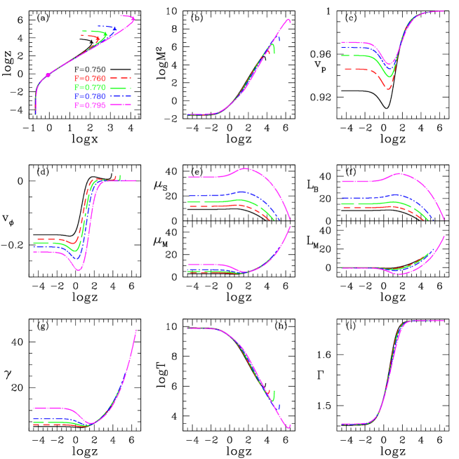
Figure 1: Outflow solutions for different values of $F=0.750(\mbox{solid black})$, $0.760(\mbox{dashed red})$, $0.770(\mbox{long-dashed green})$, $0.780(\mbox{dashed-dotted blue})$, $0.795(\mbox{long-dashed-dotted magenta})$ and other four parameters are fixed i.e., $x^{2}_{A}=0.75,\theta_{A}=50,\psi_{A}=55,q=500,\xi=1$. (a) Projected stream line, (b) $log(M^{2})$, (c) $v_{\rm p}$, (d) $v_{\phi}$, (e) $\mu_{S}=-\varpi\Omega B_{\phi}/\Psi_{A}c^{2}$ and $\mu_{M}=\gamma h$, (f) $L_{B}$ and $L_{M}$, (g) $\gamma$, (h) $log(T)$ and (i) $\Gamma$, are plotted with $log(z)$. Here, $z$ is vertical height and $x$ is cylindrical radius in units of light cylinder. Solid circles and triangles represent Alfvén point and fast-point locations.

In this paper, the velocity is measured in the units of speed of light $c$ and distance is in units of light cylinder $r_{c}\equiv\frac{c}{\Omega}$. In our model, there are two main free input parameters $F$ and $q$, three boundary parameters $\psi_{A},\theta_{A},x^{2}_{A}$ and a composition parameter $\xi$. We study the effect of these parameters on the outflow solutions and on the collimation of outflowing matter with relativistic EoS.

4.1 Solutions for different current distributions ($F$)

In Fig.1, we plot different solutions for different current distribution parameter $F=0.750$ (solid black), $0.760~{}(\mbox{dashed red})$, $0.770~{}(\mbox{long-dashed green})$, $0.780~{}(\mbox{dashed-dotted blue})$, $0.795~{}(\mbox{long-dashed-dotted magenta})$ and other four parameters are fixed i.e., $x^{2}_{A}=0.75,~{}\theta_{A}=50,~{}\psi_{A}=55,~{}q=500$ & $\xi=1.0$. In Fig.1a, projected stream line in the $x-z$ plane is plotted. The distribution of corresponding flow variables like $log(M^{2})$ (Fig.1b), poloidal velocity $v_{\rm p}$ (Fig.1c), azimuthal velocity $v_{\phi}$ (Fig.1d), Poynting to mass flux ratio $\mu_{S}\equiv-\varpi\Omega B_{\phi}/\Psi_{A}c^{2}$ and matter to mass flux ratio $\mu_{M}\equiv\gamma h$ (Fig.1e), angular momentum associated with the magnetic field $L_{B}\equiv-\varpi B_{\phi}/\Psi_{A}$ and matter $L_{M}\equiv h\gamma\varpi v_{\phi}$ (Fig.1f), Lorentz factor $\gamma$ (Fig.1g), $log(T)$ (Fig.1h) and adiabatic index $\Gamma$ (Fig.1i) with $log(z)$ are plotted. In Fig.1(a), solid-circles represent Alfvén point location and solid-triangles represent the fast point location, where $z$ is the vertical height and $x$ is the cylindrical radius. In Fig.1(a), we note that if we increase $F$, the solution collimates at higher height $(z)$. Higher value of $F$ implies weaker magnetic field near the base, so it travels larger $z$ before the outflow starts to collimate. In panel Fig.1(c), we see that $v_{\rm p}$ has a dip, which is due to the interaction of magnetic field with matter. Near the base, $\mu_{S}$ gains at the cost of $\mu_{M}$ (Fig.1e), therefore there is simultaneous decrease in thermal and kinetic terms. When the magnetic energy ($\mu_{S}$) becomes sufficiently strong, it starts to accelerate the outflow, although the outflow temperature continue to decrease. Hence there is a dip in $v_{\rm p}$. Another very interesting result is that $v_{\phi}$ changes sign from negative to positive (Fig.1d). It means, initially the flow is rotating clockwise and somewhere in between the Alfvén and the fast points, the flow flips to a counter-clockwise direction. In MHD, we have two types of angular momentum, one that is associated with the matter $L_{M}\equiv h\gamma\varpi v_{\phi}$ and the other associated with the magnetic field $L_{B}\equiv-\varpi B_{\phi}/\Psi_{A}$. Therefore, only total angular momentum is conserved throughout the flow but not the individual angular momenta (Fig.1f). Thus, azimuthal velocity $v_{\phi}$ changes sign because of transfer of angular momentum from magnetic field to matter. In Fig.1(g), the variation of Lorentz factor $\gamma$ is shown. We can see that higher value of $F$ produces outflows with higher Lorentz factor $\gamma\sim 45$ ($F=0.795,\mbox{ long-dashed-dotted}$). In Fig.1(h), we plot temperature variation of the outflow with height, for different values of $F$ parameter. We can see that outflow starts with high temperature when it is sub-Alfvénic and temperature drops to very small value when the flow becomes super-fast. Last panel Fig.1(i) shows that the adiabatic index $\Gamma$ does not remain constant throughout the solution, it varies from $\Gamma\sim~{}1.44$ to $5/3$. It is well known that gases with non-relativistic temperatures have $\Gamma=5/3$ or the polytropic index $N=3/2$. For gases with ultra-relativistic temperatures, $N\rightarrow 3$ or $\Gamma\rightarrow 4/3$. It may be noted that, $N$ is the temperature gradient of the specific energy of the gas i.e., $\sim df/d\Theta$ (see, equation 5). For non-relativistic thermal speed (for $T\lower 2.15277pt\hbox{$\;\buildrel<\over{\sim}\;$}10^{7}$K, the energy density of the gas (${\bar{e}}$) is dominated by rest-mass energy, so $N$ (therefore $\Gamma$) remains constant ($\equiv 5/3$). But for higher temperatures, the thermal speed becomes relativistic, therefore kinetic contribution becomes comparable to rest mass in ${\bar{e}}$, as a result $N$ increases with rising $T$. But the upper limit of thermal speed is $c$, therefore for ultra-relativistic temperature, the kinetic contribution of the gas particles into ${\bar{e}}$ of the gas becomes maximum and therefore $N$ again becomes temperature independent, where asymptotically $N\rightarrow 3$ (or, $\Gamma\rightarrow 4/3$). For example, if the temperature of a gas is in between these two extremes ($10^{7}~{}{\rm K}<T<10^{13}$K), then the thermal state is described by $3/2\lower 2.15277pt\hbox{$\;\buildrel<\over{\sim}\;$}N\lower 2.15277pt\hbox{$\;\buildrel<\over{\sim}\;$}3$ (see, figure 1a of Chattopadhyay & Ryu, 2009). In Fig.1(h), temperature drops from $\sim 10^{10}$ to $\sim 10^{4}$ the thermal energy decreases as a result, $\Gamma$ changes from $\sim 1.44$ (near-relativistic) to $\sim 5/3$ (non-relativistic).

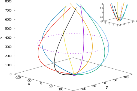
(a) Streamline side view.

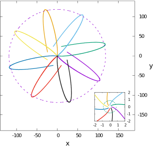
(b) Streamline top view.

Figure 2: Solid lines represent the stream lines of outflow solution for $x^{2}_{A}=0.75,\theta_{A}=50,\psi_{A}=55,F=0.75,q=500,\xi=1$. (a) Sideview and (b) top view. There are two dashed circles, one near to the center at $z\sim 0.73$ represents the Aflvén point location and second at $z\sim 3500$ represents the fast point location. Here, $z$ is vertical height and $x,y$ are in terms of light cylinder. Inset: Region close to the base is zoomed to show the location of the Alfvén point (dashed circle).

In Fig. 2, we plot the stream lines of outflow solution for $x^{2}_{A}=0.75,\theta_{A}=50,\psi_{A}=55,F=0.75,q=500,\xi=1$. Figures 2(a) & (b) are the side and top view of stream lines of the outflow, respectively. Here $xy$ plane represent the equatorial plane and $z$ is the vertical height from the equatorial plane in terms of light cylinder. Two dashed circles, one near to the base $(z\sim 0.73$ i.e., the circle in the inset of both the panels) represents the Aflvén point location. The other at $z\sim 3500$ represents the fast point location. As we discussed before, the transfer of angular momentum from the field to the matter, changes the direction of rotation of the flow. We can also see in Fig. 2, that the transfer of angular momentum from field to the matter has twisted the stream lines of the outflow.

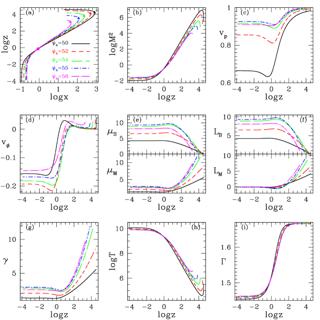
Figure 3: Outflow solutions are for different values of $\psi_{A}=50~{}(\mbox{solid black})$, $52~{}(\mbox{dashed red})$, $54~{}(\mbox{long-dashed green})$, $55~{}(\mbox{dashed-dotted blue})$, $56~{}(\mbox{long-dashed-dotted magenta})$. All the curves plotted are for $x^{2}_{A}=0.75,~{}\theta_{A}=50,~{}F=0.75,~{}q=500,~{}\&~{}\xi=1$. Panel (a) Stream line on the $xz$-plane, (b) $[log(M^{2})]$, (c) $v_{\rm p}$, (d) $v_{\phi}$, (e) $\mu_{S}$ and $\mu_{M}$, (f) $L_{B}$ and $L_{M}$, (g) $\gamma$, (h) $log(T)$ and (i) $\Gamma$ versus $log(z)$. Here, solid circles and triangles represent Alfvén and fast point locations.

4.2 Solutions for different Alfvén point angle ($\psi_{A}$) with the disk

In Fig.3 we plot outflow solutions for different values of $\psi_{A}=50~{}(\mbox{solid, black})$, $52~{}(\mbox{dashed, red})$, $54~{}(\mbox{long-dashed, green})$, $55~{}(\mbox{dashed-dotted, blue})$ and $56$ (long-dashed-dotted, magenta). All the curves are for fixed values of $x^{2}_{A}=0.75,\theta_{A}=50,F=0.75,q=500$ and $\xi=1$. In Fig.3(a), the solution which has lower values of $\psi_{A}$ are less collimated. Since, centrifugal force also has component in the poloidal direction i.e., $cos(\psi)$ component of centrifugal force (see equation 20 in Vlahakis et al., 2003a), therefore flow which has small Alfvén point angle with the equatorial plane has larger centrifugal force which spreads the outflow over larger $x$. In general, the solutions with lower $\psi_{A}$, are of lower $\mu$ and $\sigma_{M}$ and therefore are slower (i.e., less $v_{\rm p}$). Although $\mu$ and $L$ are constants of motion, but respective magnetic and matter components of each are not constants. The azimuthal component of velocity $v_{\phi}$ also flips sign. Panels Fig.3(h-i) show the variation of temperature and adiabatic index (varies from $1.4$ to $5/3$) of the flow.

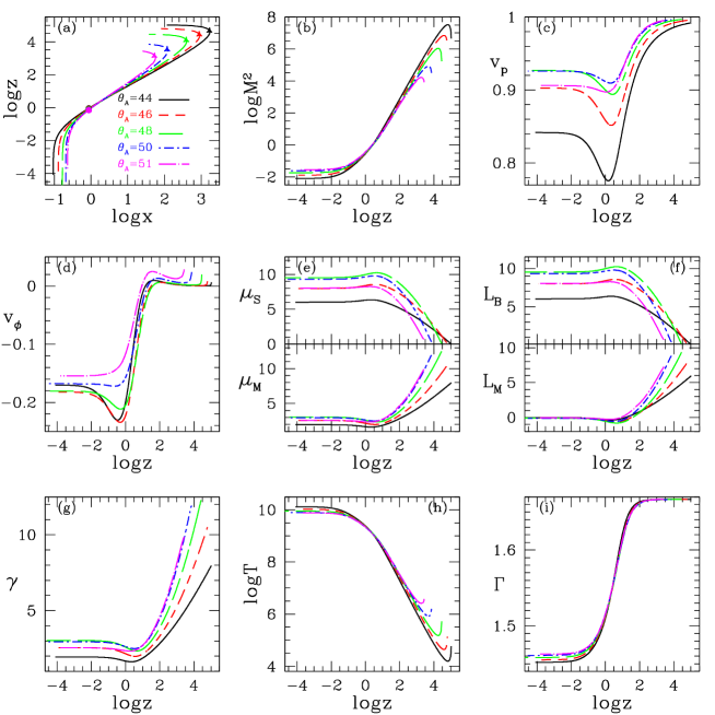
Figure 4: Outflow solutions for different values of $\theta_{A}=44~{}(\mbox{solid black})$, $46~{}(\mbox{dashed red})$, $48~{}(\mbox{long-dashed green})$, $50~{}(\mbox{dashed-dotted blue})$, $51~{}(\mbox{long-dashed-dotted magenta})$ and four parameters are fixed i.e., $x^{2}_{A}=0.75,\psi_{A}=55,F=0.75,q=500,\xi=1$ for all the curves. Panel (a) Stream line on the $xz$-plane, (b) $[log(M^{2})]$, (c) $v_{\rm p}$, (d) $v_{\phi}$, (e) $\mu_{S}$ and $\mu_{M}$, (f) $L_{B}$ and $L_{M}$, (g) $\gamma$, (h) $log(T)$ and (i) $\Gamma$ versus $log(z)$. Here, solid circles and triangles represent Alfvén and fast point locations.

4.3 Solutions for different Alfvén point polar angle ($\theta_{A}$)

In Fig.4, we plot outflow solutions for different values of $\theta_{A}=44~{}(\mbox{solid black})$, $46~{}(\mbox{dashed red})$, $48~{}(\mbox{long-dashed green})$, $50~{}(\mbox{dashed-dotted blue})$, $51~{}(\mbox{long-dashed-dotted magenta})$. Five parameters are fixed $x^{2}_{A}=0.75,~{}\psi_{A}=55,~{}F=0.75,~{}q=500$ and $\xi=1$ for all the curves. Solutions with smaller $\theta_{A}$ start with a smaller base (small $x$), but expands to a larger $x$. While the ones starting with larger $\theta_{A}$ shows exactly the opposite property. This is because the solution with smaller $\theta_{A}$ have larger value of $B_{\phi}$ near the base, but at higher $z$, $B_{\phi}$ decreases faster than the one starting with higher values of $\theta_{A}$. In general, $v_{\rm p}$ of outflow solution is higher for higher value of $\theta_{A}$ ($51\mbox{ long-dashed-dotted, magenta}$). The $\mu_{S}$ and $\mu_{M}$ feeds at each others cost, although the total specific energy $\mu$ remains constant along the flow. This is similar to the constancy of the total angular momentum of the flow, but components associated with the field and the matter are not constant. As in the previous cases, here too the adiabatic index is not constant.

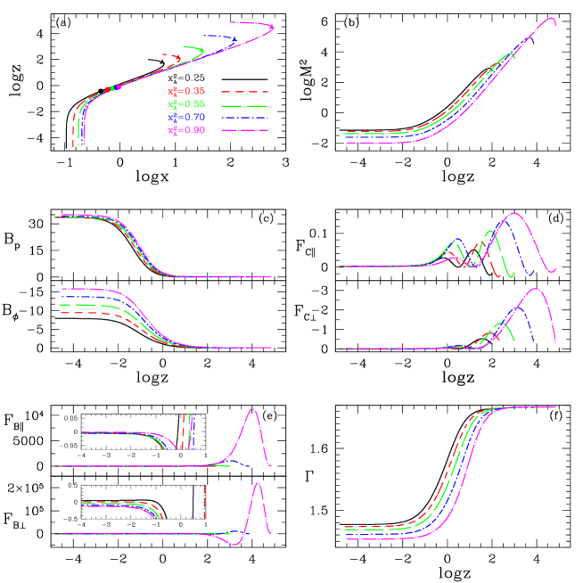
Figure 5: Outflow solutions are for different values of $x^{2}_{A}=0.25~{}(\mbox{solid black})$, $0.35~{}(\mbox{dashed red})$, $0.55~{}(\mbox{long-dashed green})$, $0.70~{}(\mbox{dashed-dotted blue})$, $0.90~{}(\mbox{long-dashed-dotted magenta})$. All the curves are plotted for fixed values of $\theta_{A}=50,~{}\psi_{A}=55,~{}F=0.75,~{}q=500,~{}\&~{}\xi=1$. Panel (a) Stream line on the $xz$-plane, (b) $log(M^{2})$, (c) $B_{\rm p}$ and $B_{\phi}$, (d) $F_{{\rm C}\parallel}$ and $F_{{\rm C}\perp}$, (e) $F_{{\rm B}\parallel}$ and $F_{{\rm B}\perp}$, (f) $\Gamma$ versus $log(z)$. Here, solid circles and triangles in panel (a), represent Alfvén and fast point locations. The inset in panel (e) zooms on to various curves corresponding to different values of $x_{A}$.

4.4 Solutions for different Alfvén point cylindrical radius ($x_{A}$)

In Fig. 5, we plot outflow solutions for different values of $x^{2}_{A}=0.25~{}(\mbox{solid black})$, $0.35~{}(\mbox{dashed red})$, $0.55~{}(\mbox{long-dashed green})$, $0.70~{}(\mbox{dashed-dotted blue})$, $0.90$ (long-dashed-dotted, magenta). And other parameters which are kept fixed for all the curves are $\theta_{A}=50,\psi_{A}=55,F=0.75,q=500$ and $\xi=1$. The poloidal ($B_{\rm p}$) as well as toroidal magnetic ($B_{\phi}$) fields are higher for flows of higher $x_{A}$. However at larger $z$, both the components of the magnetic field fall faster, compared to that in the flows of lower $x_{A}$ (see Fig. 5c). Moreover, the component of centrifugal and magnetic forces along the streamline ($F_{{\rm C}\parallel}~{}\&~{}F_{{\rm B}\parallel}$) are larger for higher values of $x_{A}$. On the other hand, collimation is achieved due to the competition between the components of magnetic ($F_{{\rm B}\perp}$) and centrifugal ($F_{{\rm C}\perp}$) forces orthogonal to the streamline (Fig. 5a, d, e). As a result, solutions corresponding to lower values of $x_{A}$ are more collimated (Figs.5a), because the resultant of magnetic and centrifugal forces are directed towards the axis, closer to the base than those with larger values of $x_{A}$. This is expected due to the assumption of radial self-symmetry. The $\Gamma$ distribution along the streamline for different values of $x_{A}$, varies significantly from each other (Fig. 5f). It may be noted that, in almost all the cases, the outflow crosses the light cylinder with impunity.

4.5 Comparison of solutions for fixed and variable adiabatic index EoS (CR EoS)

In this section, we compared solutions of fixed adiabatic index EoS (with $\Gamma=5/3$ and $4/3$) and CR EoS.

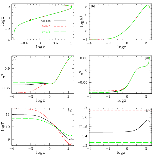
Figure 6: Outflow solutions with variable adiabatic index CR EoS (solid black) with $\xi=1$, fixed adiabatic index EoS with $\Gamma=5/3~{}(\mbox{dashed red})$, and $\Gamma=4/3~{}(\mbox{long-dashed green})$. All curves are plotted for $\mu=2.82420$, $x^{2}_{A}=0.25,~{}\theta_{A}=52,~{}\psi_{A}=55,$ and $F=0.8$. Panel (a) Stream line on the $xz$-plane, (b) $logM^{2}$, (c) $v_{\rm p}$, (d) $v_{\phi}$, (e) $logT$, (f) $\Gamma$ versus $log(z)$.

In Fig. 6, we plot outflow solutions for variable adiabatic index EoS or CR EoS (solid black) with $\xi=1$ and fixed adiabatic index EoS with $\Gamma=5/3~{}(\mbox{dashed red})$ and $\Gamma=4/3~{}(\mbox{long-dashed green})$. All curves are plotted for $\mu=2.82420$, $x^{2}_{A}=0.25,~{}\theta_{A}=52,~{}\psi_{A}=55,$ and $F=0.8$. Panel (a) shows the stream line on the $xz$-plane, (b) $logM^{2}$, (c) $v_{\rm p}$, (d) $v_{\phi}$, (e) $logT$, (f) $\Gamma$ versus $log(z)$. In Fig. 6a, the streamlines of all the outflow solutions for different EoS are same. Interestingly, all the solutions also pass through both Alfvén and fast critical points. These solutions also have almost similar Alfén Mach number distribution (Fig. 6b). However, in Fig. 6c, we can see that there is significant difference in the poloidal velocity and these solutions also have different values of azimuthal velocity (Fig. 6d). The solutions using CR EoS, cannot be scaled with any particular fixed value of $\Gamma$. This has been shown in many paper in the hydrodynamic (radiation hydrodynamic) limit (Chattopadhyay & Ryu, 2009; Chattopadhyay & Kumar, 2016; Kumar & Chattopadhyay, 2017; Vyas & Chattopadhyay, 2019). As is expected, solutions of different EoS have different overall temperature variation (Fig. 6e). In Fig. 6f, we present the variation of adiabatic index for CR EoS and the comparison with fixed adiabatic index. For solutions with different EoS, $T(r)$ crosses each other at some distance and yet, $\Gamma$ computed from CR EoS, is neither $5/3$ nor $4/3$. It is clear by comparing Figs. 6(e) and (f), that, the temperature obtained by using $\Gamma=4/3$ is less than that obtained by using $\Gamma=5/3$, which clearly should not be the case. Since, only very hot plasma should be described by $\Gamma=4/3$ and cold plasma ($T<10^{7}$K, i.e., $T<<m_{{\rm e}^{-}}c^{2}/k$) should be described by $\Gamma=5/3$, therefore, relativistic flows described by fixed $\Gamma$ EoS clearly has a temperature discrepancy.

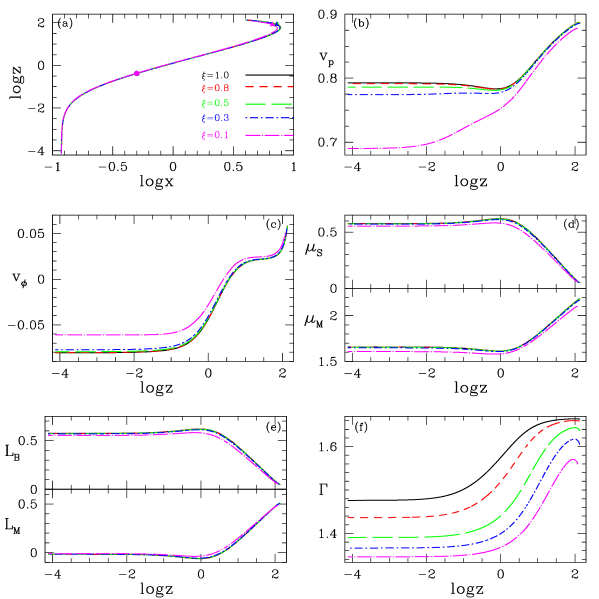
Figure 7: Outflow solutions for different values of $\xi=1.0~{}(\mbox{solid, black})$, $0.8~{}(\mbox{dashed, red})$, $0.5~{}(\mbox{long-dashed, green})$, $0.3~{}(\mbox{dashed-dotted, blue})$, $0.1~{}(\mbox{long-dashed-dotted, magenta})$. All the curves are plotted for $x^{2}_{A}=0.25,~{}\theta_{A}=50,~{}\psi_{A}=55,~{}F=0.75,$ and $q=500$. Panel (a) Stream line on the $xz$-plane, (b) $v_{\rm p}$, (c) $v_{\phi}$, (d) $\mu_{S}$ and $\mu_{M}$, (e) $L_{B}$ and $L_{M}$, (f) $\Gamma$ versus $log(z)$. Here, solid circles and triangles represent Alfvén and fast point locations.

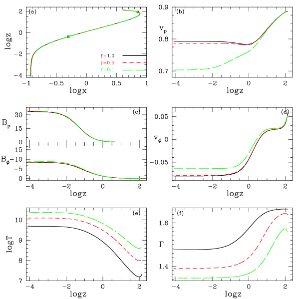
Figure 8: Outflow solutions for different values of $\xi=1.0~{}(\mbox{solid, black})$, $0.5~{}(\mbox{dashed, red})$ and $0.1~{}(\mbox{long-dashed, green})$. All the curves are plotted for $\mu=2.23362,~{}\theta_{A}=50,~{}\psi_{A}=55,~{}F=0.75,$ and $q=500$. Panel (a) Stream line on the $xz$-plane, (b) $v_{\rm p}$, (c) $B_{\rm p}$ and $B_{\phi}$, (d) $v_{\phi}$, (e) $log(T)$, (f) $\Gamma$ versus $log(z)$.

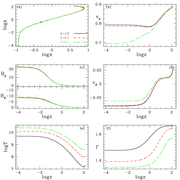
Figure 9: Outflow solutions for different values of $\xi=1.0~{}(\mbox{solid, black})$, $0.5~{}(\mbox{dashed, red})$, $0.1~{}(\mbox{long-dashed, green})$. All the curves are plotted for $L=0.55585,~{}\theta_{A}=50,~{}\psi_{A}=55,~{}F=0.75,$ and $q=500$. Panel (a) Stream line on the $xz$-plane, (b) $v_{\rm p}$, (c) $B_{\rm p}$ and $B_{\phi}$, (d) $v_{\phi}$, (e) $log(T)$, (f) $\Gamma$ versus $log(z)$.

4.6 Solutions for different plasma compositions ($\xi$)

In Fig.7 we have presented outflow solutions for different compositions, $\xi=1.0(\mbox{solid black})$ is electron-proton, $0.8(\mbox{dashed red})$, $0.5(\mbox{long-dashed green})$, $0.3~{}(\mbox{dashed-dotted blue})$, $0.1$ (long-dashed-dotted, magenta) and other five parameters are fixed i.e., $x^{2}_{A}=0.25,\theta_{A}=50,\psi_{A}=55,F=0.75,q=500$. In these solutions $\mu$ and $\sigma_{M}$ increases slightly with the increase in $\xi$, if $x_{A},~{}\theta_{A},~{}\psi_{A}$ and $q$ are kept constant. It is also reflected in the plots of $\mu_{S}$ and $\mu_{M}$, as well as $L_{B}$ and $L_{M}$ (Fig.7e, f). There is very little difference in the streamlines of the jets (Fig.7a). However, by varying the composition of the flow from electron-proton plasma (i.e., $\xi=1.0$) to pair dominated flow $\xi=0.1$, $v_{\rm p}$ and $v_{\phi}$ of the flow varies significantly with $\xi$ (Figs.7 b & c). Even $\mu_{S}$, $\mu_{M}$ and $L_{S}$,$L_{M}$ also depend on $\xi$ (Fig. 7d & e). Since $\xi$ also influences the thermodynamics of the flow, the temperature of the jet is also crucially influenced by its composition. As a result the adiabatic index $\Gamma$ also depends on $\xi$ (Fig.7f). It may be noted, that the temperature of pair-dominated flow is higher than electron-proton flow and therefore $\Gamma$ at any given $z$ is lower for flows with lower value of $\xi$. Since we are comparing flows with same $x_{A}$ (equivalently, $M_{A}$), therefore from equation 16, it can be easily shown that the temperature of pair dominated flow will be higher.

In Figs. 8, we plot magnetized outflow solutions for different compositions like $\xi=1.0$ (solid, black), $0.5$ (dashed, red) and $0.1$ (long-dashed, green), but are for the same $\mu=2.23362,~{}\theta_{A}=50,~{}\psi_{A}=55,~{}F=0.75,$ and $q=500$. So all these solutions are for the same Bernoulli parameter $\mu$. Since all other parameters are same, the magnetic field components and streamlines for each are almost the same (Figs. 8a & c), yet $v_{\rm p}$ & $v_{\phi}$ (Figs. 8b & d) distribution are completely different for flows with different $\xi$. Moreover, even the temperature ($T$) and $\Gamma$ also depend on the composition parameter (Fig. 8e & f). The baryon poor outflows which have same Bernoulli parameter, are slower and hotter, compared to electron-proton flow. However, the gain in $v_{\rm p}$ is more for pair dominated flow than the electron-proton flow.

In Figs. 9, we plot magnetized outflow solutions for different compositions like $\xi=1.0$ (solid, black), $0.5$ (dashed, red) and $0.1$ (long-dashed, green), but are for the same $L=0.55585,~{}\theta_{A}=50,~{}\psi_{A}=55,~{}F=0.75,$ and $q=500$, i. e., we compare outflows launched with the same total angular momentum (or $L$) but different $\xi$. The streamlines are again almost the same (Figs. 9a), however, $v_{\rm p}$, $v_{\phi}$, and $T$ or $\Gamma$ (Figs. 9b—f) are significantly different for flows with different $\xi$.

It may be remembered that the general expression of constants of motion $\mu$ and $L$ in physical units are (Vlahakis et al., 2003a)

$$\mu=h\gamma-\frac{\varpi\Omega B_{\phi}}{\Psi_{A}c^{2}};~{}L=\varpi\gamma hv_{\phi}-\frac{\varpi B_{\phi}}{\Psi_{A}}$$

From equation 4, it is also clear that $h$ depends on composition parameter $\xi$. So, for a given $\mu$ or $L$, if $B_{\phi}$ is somewhat similar at the base, then $\gamma$ (i.e., $v_{\rm p},~{}v_{\phi}$) and $\Theta$ will depend on $\xi$. That is exactly what we see in Figs. 8 & 9. Dependence of flow velocity and temperature on the composition of the flow, has also been shown in the hydrodynamic regime recently (Chattopadhyay & Ryu, 2009; Chattopadhyay & Kumar, 2016; Vyas & Chattopadhyay, 2019; Singh & Chattopadhyay, 2019). Therefore, it is expected that some imprint of the flow composition should be there in radiative output of the flow.

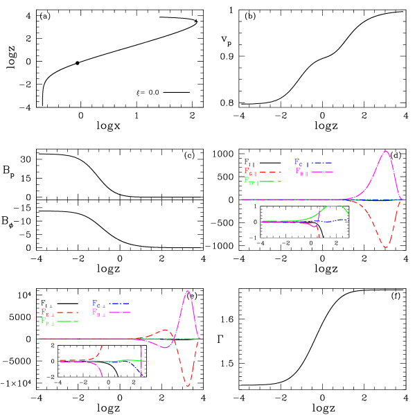
Figure 10: Outflow solutions for composition $\xi=0.0$. All the curves are plotted for $x^{2}_{A}=0.75,~{}\theta_{A}=50,~{}\psi_{A}=55,~{}F=0.75,$ and $q=0.05$. Panel (a) Stream line on the $xz$-plane, (b) $v_{\rm p}$, (c) $B_{\rm p}$ and $B_{\phi}$, (d) parallel forces, (e) perpendicular forces, (f) $\Gamma$ versus $log(z)$.

In Fig. 10, we plot an electron-positron outflow solution or flow having $\xi=0.0$. Other parameters are $x^{2}_{A}=0.75,~{}\theta_{A}=50,~{}\psi_{A}=55,~{}F=0.75,$ and $q=0.05$. From Fig. 10b, it is clear that pure leptonic flow is also a trans-fast flow and the velocity nature is similar to proton poor flows as plotted in Fig. 8b. In Fig. 10d, we plot the forces which control the poloidal acceleration of the flow, for example, parallel inertial force $F_{I\parallel}$, parallel ‘gamma’ force $F_{G\parallel}\equiv F_{GP\parallel}+F_{G\phi\parallel}$, parallel total thermal gradient force $F_{TP\parallel}\equiv F_{T\parallel}+F_{P\parallel}$, parallel centrifugal force $F_{C\parallel}$, and parallel magnetic force $F_{B\parallel}$ (for more details see section 2.2 in Vlahakis et al., 2003a). In the inset of Fig. 10d, we can note that these forces are comparable to each other at lower value of $z$, however for greater value of $z$, $F_{B\parallel}$ and $F_{G\parallel}$ forces are controlling the poloidal acceleration. In Fig. 10e, we plot all forces perpendicular to the poloidal fieldlines, e. g., $F_{I\perp}$ (inertial), $F_{E\perp}$ (electric), $F_{P\perp}$ (pressure gradient), $F_{C\perp}$ (centrifugal), and $F_{B\perp}$ (magnetic). Perpendicular forces have similar nature to parallel forces, however, at a larger distances, $F_{E\perp}$ and $F_{B\perp}$ controls the collimation of the flow. In Fig. 10f, the adiabatic index for pure lepton flow varies from $\sim 1.44$ to $\sim 5/3$.

5 Discussion and Concluding Remarks

In this paper we have solved the relativistic magneto-hydrodynamic equations using relativistic equation of state, in order to study relativistic outflows. A flow is relativistic on account of its bulk velocity (i.e., $v_{\rm p}\lower 2.15277pt\hbox{$\;\buildrel<\over{\sim}\;$}c$) and also in terms of its temperature i.e., when $kT_{i}\lower 2.15277pt\hbox{$\;\buildrel>\over{\sim}\;$}m_{i}c^{2}$ (subscript $i$ represents the type of constituent particle). The first condition arises for outflows, far away from a black hole, but the second condition especially arises in the region close to a black hole horizon which acts as the base of an astrophysical jet. A form of EoS (CR) of a flow which can transit between relativistic to non-relativistic temperatures has been used in this paper. As has been discussed through out this paper, $\Gamma$ is a function of temperature in CR EoS and is automatically determined from temperature distribution. There are a few papers in hydrodynamic regime (read in absence of ordered magnetic field) which discusses the application of relativistic EoS in accretion and jets (Chattopadhyay & Kumar, 2016; Kumar & Chattopadhyay, 2017; Vyas & Chattopadhyay, 2019). However, as far as we know, there have been no such previous attempts to solve relativistic, trans-Alfvénic, trans-magneto sonic plasma expressed by relativistic EoS and study the effect of different compositions of the plasma. Since MHD equations are only applicable for fully ionized plasma, therefore, the composition of the flow is likely to either be electron-proton ($\xi=1$) plasma or electron-positron-proton ($0<\xi<1$) plasma. In this paper, we have studied how various parameters like the Bernoulli constant, current distribution, the location of the Alfvén point etc affect the outflow solution but only for electron-proton plasma. And then studied the effect of different EoS and different compositions on outflow solutions.

We investigated the contribution played by all the flow parameters, information of which shapes the final solution of the outflow. We found that the current distribution affects the stream line structure, as well as the flow velocities, especially close to the base. We also found that, not only the current distribution, the angle of the poloidal fieldline makes with the equatorial plane also affect the solutions. In particular, the streamlines which are more inclined to the equatorial plane are slower and less collimated. In addition, narrower the polar angle of the Alfvén point with the axis of the flow, slower and less collimated is the outflow. These two angles, namely $\psi_{A}$ and $\theta_{A}$ are independent of each other. For a given composition, the location of the Alfvén point has significant effect on the Bernoulli parameter $\mu$, the streamline and the Lorentz factor of the flow. We found that while the $q$ parameter which depends on the entropy, itself do not explicitly affect the outflow solutions significantly except the temperature, but in conjunction with other parameters plays an important role.

We have also compared the outflow solutions using fixed adiabatic index EoS, with the one using CR EoS for a given value of $\mu$, $x_{A}$, $\theta_{A}$, $\Psi_{A}$ and $F$. Although the streamlines are similar, but distribution of flow variables ($v_{\rm p}$, $v_{\phi}$, and $T$) are significantly different. Interestingly, solutions of all the EoS, are passed through both the critical points (Alfvén and fast magnetosonic). It may be noted, that Vlahakis et al. (2003a, b) only obtained trans-Alfvénic outflow using $\Gamma=4/3$, but Polko et al. (2010) obtained trans-Alfvénic, trans-fast outflow solutions using $\Gamma=5/3$. However, we showed that even with $\Gamma=4/3$, one can obtain trans-Alfvénic, trans-fast outflow solution (Fig. 6a). It appears that, depending on the values of other parameters, there exists a critical value of $F$, below which the flow passes through both the critical points, but for higher values of $F$, the outflow is only trans-Alfvénic in nature. For example for the parameters related to Fig. 1, trans-Alfvénic, trans-fast outflow is possible if $F<0.82$.

We showed that, jets of all composition passes through the Alfvén and the fast point, and get collimated to the axis after crossing the fast point. We compared solutions with different composition, but for the same values of the Alfvén point, or the Bernoulli constant, or the total angular momentum. In all the cases, composition has little effect on the streamlines, but $v_{\rm p}$, $v_{\phi}$ and $T$ distributions are significantly different. It means that the electro-magnetic output of such outflows should also depend on the composition. Since pair-plasma have been regularly invoked as the composition of jets, we have also presented one case of pure pair plasma (i. e., $\xi=0.0$) outflow solution and it nicely passes through the both critical points. The pair plasma outflow accelerates mainly in the sub-Alfvénic region to super-fast region. The effect of composition is quite pronounced in presence of gravity as was seen in the hydrodynamic limit (Chattopadhyay & Ryu, 2009; Kumar et al., 2013; Chattopadhyay & Kumar, 2016) as well as, in the non-relativistic MHD regime (Singh & Chattopadhyay, 2018, 2019). So we expect the effect of CR EoS will be more pronounced in the RMHD limit, if gravity is considered. However, presently consideration of gravity is beyond the scope of this paper. It may be noted that RMHD equations combined with pseudo-Newtonian gravity have been used to study outflows previously, with very interesting results (Polko et al., 2013, 2014; Ceccobello et al., 2018). In this paper, the jet only passes through two critical points (Alfvén and fast) and not the slow. The slow point appears in presence of gravity. The existence of slow-magnetosonic point ensures low velocity and high temperature at the base of jet, or in other words, corrects the boundary condition at the jet base.

In all the solutions, the jet stream lines show that there is a possibility that after crossing the fast point, over collimation/magnetic field pinching can produce shock. Since the flow is moving with super-fast speed, so formation of shock is not going to affect the flow in the upstream and this shock location can be related to the fast point location. In case of M87, Asada & Nakamura (2012) showed that jet radius versus jet height nicely fit parabolic curve up to $5\times 10^{5}r_{g}$ height and after this jet radius versus height follow conical structure. There is a dip in jet radius near the HST-1 which is located at $5\times 10^{5}r_{g}$ i.e., jet radius versus height departs from parabolic structure and this may be due to collimation shock.

Appendix A Equations of motion

The Bernoulli equation ($\mu=\gamma h-\varpi\Omega B_{\phi}/\Psi_{A}c^{2}$) is obtained from the identity $\gamma^{2}\left(1-v^{2}_{\phi}/c^{2}\right)=1+\gamma^{2}v^{2}_{p}/c^{2}$ (for more details see Vlahakis et al. (2003a)),

$$\mu^{2}=\left(h^{2}+\frac{F^{2}\sigma^{2}_{M}M^{4}\mbox{sin}^{2}\theta}{x^{4}\mbox{cos}^{2}(\theta+\psi)}\right)\times\left(\frac{G^{4}(1-M^{2}-x^{2})^{2}}{G^{4}(1-M^{2}-x^{2}_{A})^{2}-x^{2}(G^{2}-M^{2}-x^{2})^{2}}\right).$$ (21)

Because $\mbox{tan}\psi=\frac{\partial z}{\partial\varpi}=\frac{d(G/\mbox{\small tan}\theta)}{dG}$, therefore we have,

$$\frac{dG^{2}}{d\theta}=\frac{2G^{2}\mbox{cos}\psi}{\mbox{sin}\theta\mbox{cos}(\theta+\psi)}.$$ (22)

The transfield equation is obtained from the momentum equation by taking dot product with $-\nabla A$ then by using equation (18) we can write it as,

$$G\mbox{sin}^{2}\theta\frac{d}{d\theta}\left[\mbox{tan}(\theta+\psi)\frac{1-M^{2}-x^{2}}{G}\right] = (F-1)\frac{x^{4}_{A}\mu^{2}x^{2}}{F^{2}\sigma^{2}_{M}}\left(\frac{1-G^{2}}{1-M^{2}-x^{2}}\right)^{2}$$ (23)

$$-\mbox{sin}^{2}\theta\left(\frac{M^{2}+Fx^{2}-F+1}{\mbox{cos}^{2}(\theta+\psi)}\right)$$

$$-\frac{x^{4}_{A}\mu^{2}x^{2}}{F^{2}\sigma^{2}_{M}M^{2}}\left(\frac{G^{2}-M^{2}-x^{2}}{1-M^{2}-x^{2}}\right)^{2}$$

$$+2\left(\frac{F-2}{F^{2}\sigma^{2}_{M}}\right)\left(\frac{2\Theta hx^{4}}{KM^{2}}\right)$$

By following Vlahakis et al. (2003a), the slope of $M^{2}_{A}$ at the Alfvén point i.e., $p_{A}=dM^{2}/d\theta|_{x_{A}}$ and Bernoulli equation (21) at Alfvén point is given by,

$$p_{A}=dM^{2}/d\theta|_{x_{A}}=\frac{2x^{2}_{A}\mbox{cos}\psi_{A}}{\sigma_{A}\mbox{sin}\theta_{A}\mbox{cos}(\theta_{A}+\psi_{A})}$$ (24)

and

$$\mu^{2}=\left(h^{2}_{A}+\frac{F^{2}\sigma^{2}_{M}(1-x^{2}_{A})^{2}\mbox{sin}^{2}\theta_{A}}{x^{4}_{A}\mbox{cos}^{2}(\theta_{A}+\psi_{A})}\right)\times\left(\frac{x^{2}_{A}(\sigma_{A}+1)^{2}}{x^{2}_{A}-[x^{2}_{A}-\sigma_{A}(1-x^{2}_{A})]^{2}}\right)$$ (25)

The Alfvén point condition is derived from equations (23) and (25) (see Vlahakis et al. (2003a)),

$$\frac{F^{2}\sigma^{2}_{M}(1-x^{2}_{A})(\sigma_{A}+1)^{2}}{\mu^{2}\mbox{cos}(\theta_{A}+\psi_{A})}\bigg{[}-2(F-2)\frac{2\Theta_{A}}{K}\frac{(1-x^{2}_{A})}{h_{A}x^{2}_{A}}\mbox{sin}\theta_{A}$$

$$+\frac{2\mbox{cos}\psi_{A}\mbox{sin}(\theta_{A}+\psi_{A})(\sigma_{A}+1)}{\sigma_{A}}+\frac{\mbox{sin}\theta_{A}}{x^{2}_{A}}\left[(1-x^{2}_{A})(F-1)-1\right]\bigg{]} = \left[x^{2}_{A}-(1-x^{2}_{A})\sigma_{A}\right]^{2}$$

$$-(F-1)\sigma_{A}^{2}(1-x^{2}_{A})-2\left(\frac{F-2}{h_{A}}\right)\left(\frac{2\Theta_{A}}{K}\right)\left(x^{2}_{A}-\left[x^{2}_{A}-\sigma_{A}(1-x^{2}_{A})\right]^{2}\right)$$ (26)

The coefficients of equation (18) are,

$$A_{1}=\frac{\mu^{2}x^{6}_{A}}{F^{2}\sigma^{2}_{M}}\left(\frac{M^{2}}{G^{2}}\right)\frac{(1-G^{2})^{2}}{(1-M^{2}-x^{2})^{3}}\frac{\mbox{cos}^{3}(\theta+\psi)}{\mbox{sin}^{2}\theta\mbox{sin}(\theta+\psi)}+\frac{M^{2}}{G^{4}}\frac{\mbox{cos}(\theta+\psi)}{\mbox{sin}(\theta+\psi)}$$

$$-\frac{x^{4}_{A}}{F^{2}\sigma^{2}_{M}}\frac{h^{2}}{M^{2}}\left(\frac{2\Gamma\Theta}{hK-2\Gamma\Theta}\right)\frac{\mbox{cos}^{3}(\theta+\psi)}{\mbox{sin}^{2}\theta\mbox{sin}(\theta+\psi)},$$ (27)

$$B_{1} = \frac{M^{4}}{G^{4}}$$ (28)

$$C_{1} = \frac{h^{2}x^{4}_{A}}{F^{2}\sigma^{2}_{M}}\frac{\mbox{cos}\psi\mbox{cos}^{2}(\theta+\psi)}{\mbox{sin}^{3}\theta\mbox{sin}(\theta+\psi)}\Bigg{\{}\frac{\mu^{2}G^{4}(1-M^{2}-x^{2}_{A})^{2}}{h^{2}G^{4}(1-M^{2}-x^{2})^{2}}-1$$ (29)

$$+\frac{2x^{2}}{1-M^{2}-x^{2}}\frac{\mu^{2}}{h^{2}}\left[X-Y\right]\Bigg{\}}.$$

Here

$$X=\frac{G^{4}(1-M^{2}-x^{2}_{A})^{2}-x^{2}(G^{2}-M^{2}-x^{2})^{2}}{G^{4}(1-M^{2}-x^{2})^{2}}$$

$$Y=\frac{G^{2}(G^{2}-M^{2}-x^{2})(1-M^{2}-x^{2})(1-x^{2}_{A})}{G^{4}(1-M^{2}-x^{2})^{2}}$$

The coefficients of transfield equation (23) after simplification using the expressions of $A_{1},B_{1}$ and $C_{1}$,

$$A_{2}=-\mbox{sin}^{2}\theta\mbox{tan}(\theta+\psi),$$ (30)

$$B_{2}=\frac{\mbox{sin}^{2}\theta(1-M^{2}-x^{2})}{\mbox{cos}^{2}(\theta+\psi)},$$ (31)

$$C_{2} = -\frac{\mbox{sin}^{2}\theta(1-M^{2}-x^{2})}{\mbox{cos}^{2}(\theta+\psi)}+\mbox{sin}^{2}\theta\mbox{tan}(\theta+\psi)\left[x^{2}_{A}\frac{dG^{2}}{d\theta}+(1-M^{2}-x^{2})\frac{1}{G}\frac{dG}{d\theta}\right]$$ (32)

$$+(F-1)\frac{x^{4}_{A}\mu^{2}x^{2}}{F^{2}\sigma^{2}_{M}}\left(\frac{1-G^{2}}{1-M^{2}-x^{2}}\right)^{2}-\mbox{sin}^{2}\theta\frac{M^{2}+Fx^{2}-F+1}{\mbox{cos}^{2}(\theta+\psi)}$$

$$-\frac{x^{4}_{A}\mu^{2}x^{2}}{F^{2}\sigma^{2}_{M}M^{2}}\left(\frac{G^{2}-M^{2}-x^{2}}{1-M^{2}-x^{2}}\right)^{2}+2\frac{F-2}{F^{2}\sigma^{2}_{M}}\left(\frac{2\Theta hx^{4}}{KM^{2}}\right).$$

References

- Asada & Nakamura (2012) Asada, K., & Nakamura, M. 2012, ApJ, 745, L28
- Blandford et al. (1982) Blandford, R. D., & Payne, D. G. 1982, MNRAS, 199, 883
- Ceccobello et al. (2018) Ceccobello C. et al., 2018, MNRAS, 473, 4417
- Chandrasekhar (1938) Chandrasekhar, S., 1938, An Introduction to the Study of Stellar Structure (NewYork, Dover).
- Cox & Giuli (1968) Cox J. P., Giuli R. T., 1968, Principles of Stellar Structure, Vol. 2. Gordon and Breach Science Publishers, New York
- Chattopadhyay & Chakrabarti (2000) Chattopadhyay I., Chakrabarti S. K., 2000, Int. Journ. Mod. Phys. D, 9, 57
- Chattopadhyay (2005) Chattopadhyay I., 2005, MNRAS, 356, 145
- Chattopadhyay & Ryu (2009) Chattopadhyay I., Ryu D., 2009, ApJ, 694, 492
- Chattopadhyay & Kumar (2016) Chattopadhyay I., Kumar R., 2016, MNRAS, 459, 3792.
- Ferrari et. al. (1985) Ferrari A., Trussoni E., Rosner R., Tsinganos K., 1985, ApJ, 294, 397
- Heinemann & Olbert (1978) Heinemann M., Olbert S., 1978, J. Geophys. Res., 83, 2457
- Karino, Kino & Miller (2008) Karino S., Kino M., Miller J. C., 2008, Prog. Theor. Phys., 119, 739
- Kumar et al. (2013) Kumar R., Singh C. B., Chattopadhyay I. Chakrabarti S. K., 2013, MNRAS, 436, 2864.
- Kumar & Chattopadhyay (2017) Kumar R., Chattopadhyay I., 2017, MNRAS, 469, 4221
- Lee et. al. (2016) Lee S. J., Chattopadhyay I., Kumar R., Hyung S., Ryu D., 2016, ApJ, 831, 33
- Li et. al. (1992) Li, Z.-Y., Chiueh, T., & Begelman, M. C. 1992, APJ, 394, 459
- Lii et. al. (2012) Lii P., Romanova M., Lovelace R., 2012, MNRAS, 420, 2020
- Lovelace et. al. (1986) Lovelace R. V. E., Mehanian C., Mobarry C. M., Sulkanen M. E., 1986, ApJ, 62, 1.
- Lovelace et. al. (1991) Lovelace R. V. E., Berk H. L., Contopoulos J., 1991, ApJ, 379, 696
- Meliani et. al. (2004) Meliani Z., Sauty C., Tsinganos K., Vlahakis N., 2004, A&A, 425, 773
- Michel (1969) Michel F. C., 1969, ApJ, 158, 727
- Paczyńskii & Wiita (1980) Paczyński B., Wiita P. J., 1980, A&A, 88, 23
- Pearson et. al. (1981) Pearson T. J. et. al., 1981, Nature 290, 365
- Polko et al. (2010) Polko P., Meier D. L., Markoff S. 2010, APJ, 723, 1343 (Paper I)
- Polko et al. (2013) Polko P., Meier D. L., Markoff S. 2013, MNRAS, 428, 587
- Polko et al. (2014) Polko P., Meier D. L., Markoff S. 2014, MNRAS, 438, 959
- Proga & Kalman (2004) Proga D., Kallman T. R., 2004, ApJ, 616, 688
- Ryu et. al. (2006) Ryu D., Chattopadhyay I., Choi E., 2006, ApJS, 166, 410.
- Sakurai (1985) Sakurai T. 1985, A&A, 152, 121
- Sakurai (1987) Sakurai T. 1987, PASJ, 39, 821
- Sarkar & Chattopadhyay (2019) Sarkar S., Chattopadhyay I., 2019, Int. Journ. Mod. Phys. D, 28 (2), 1950037
- Sauty et. al. (2002) Sauty C., Trussoni E., & Tsinganos K., 2002, A&A, 389, 1068.
- Singh & Chattopadhyay (2018) Singh K., Chattopadhyay I., 2018, MNRAS, 476, 4123.
- Singh & Chattopadhyay (2019) Singh K., Chattopadhyay I., 2019, MNRAS, 486, 3506
- Synge (1957) Synge J. L., 1957, The Relativistic Gas. North Holland Publ. Co., Amsterdam
- Tsinganos (2010) Tsinganos K., 2010, Mem. S. A. It. Suppl, 15, 102
- Vlahakis et. al. (2000) Vlahakis N., Tsinganos K., Sauty C., Trussoni E., 2000, MNRAS, 318, 417.
- Vlahakis et al. (2003a) Vlahakis N., Konigl A., 2003a, ApJ, 596, 1080
- Vlahakis et al. (2003b) Vlahakis N., Konigl A., 2003b, ApJ, 596, 1104
- Vyas et. al. (2015) Vyas M. K., Kumar R., Mandal S., Chattopadhyay I., 2015, MNRAS, 453, 2992.
- Vyas & Chattopadhyay (2017) Vyas M. K., Chattopadhyay I., 2017, MNRAS, 469, 3270.
- Vyas & Chattopadhyay (2018) Vyas M. K., Chattopadhyay I., 2018, A&A, 614, A51.
- Vyas & Chattopadhyay (2019) Vyas M. K., Chattopadhyay I., 2019, MNRAS, 482, 4203.
- Weber & Davis (1967) Weber E. J., Davis L. J., 1967, ApJ, 148, 217.