Chiral susceptibility in Nambu Jona Lasinio model: a Wigner function approach

Abstract

We estimate here chiral susceptibility at finite temperature within the framework of the Nambu-Jona-Lasinio model (NJL) using the Wigner function approach. We also estimate it in the presence of chiral chemical potential ($\mu_{5}$) as well as a non vanishing magnetic field ($B$). We use medium separation regularization scheme (MSS) to calculate the chiral condensate and corresponding susceptibility. It is observed that for a fixed value of chiral chemical potential ($\mu_{5}$), transition temperature increases with the magnetic field. While for the fixed value of the magnetic field, transition temperature decreases with chiral chemical potential. For a strong magnetic field, we observe non degeneracy in susceptibility for up and down type quarks.

I INTRODUCTION

In recent years extensive efforts have been made to create and understand strongly interacting matter in relativistic heavy ion collision experiments e.g. at relativistic heavy ion collider (RHIC) and at large hadron collider (LHC). There are mounting evidences which indicate formation of deconfined quark gluon plasma (QGP) phase of quantum chromodynamics (QCD) in the initial stages of these experiments as well as the formation of confined hadron phase in the subsequent evolution of QGP. Ground state of QCD exhibits two main non perturbative features, color confinement and spontaneous breaking of chiral symmetry. The dynamical breaking of chiral symmetry is the manifestation of the quark-antiquark condensation in the QCD vacuum. Dynamical chiral symmetry breaking characterizes the non perturbative nature of QCD vacuum at vanishing temperature and/or density. With increase in temperature and/or baryon density, the QCD vacuum undergoes a transition from a chiral symmetry broken phase to a chiral symmetric phase. This transition is characterized by the quark-antiquark scalar condensate, the order parameter of the chiral phase transition. Although for first order phase transition order parameter changes discontinuously across the transition point, for second order phase transition or for a cross over transition the variation of order parameter across the transition point is rather smooth. In these cases the fluctuation of this order parameter and the associated susceptibilities are more relevant for the characterization of the thermodynamic properties of the system.

The characteristics of fluctuations and correlations are intimately connected to the phase transition dynamics, e.g. fluctuations of all length scales are relevant at QCD critical point where the first order quark-hadron phase transition line ends. The study of fluctuations and correlations are essential phenomenological tool for the experimental exploration of the QCD phase diagram. In the context of heavy-ion collisions by studying the net electric charge fluctuation, it has been demonstrated that net electric charges are suppressed in the QGP phase as compared to the hadronic phase chargefluc1 ; chargefluc2 . It has also been pointed out that the correlation between baryon number and strangeness is stronger in the QGP phase as compared to the hadronic phase strangenessenhancement1 ; strangenessenhancement2 . The quantity of interest here is the chiral susceptibility which measures the response of the chiral condensate to the variation of the current quark mass. Chiral susceptibility has been calculated using first principle lattice QCD (LQCD) simulations lattice1 ; lattice2 ; lattice3 ; lattice4 ; lattice5 ; lattice6 . All these lattice results show a pronounced peak in the variation of chiral susceptibility with temperature at the transition temperature, which essentially characterizes the chiral transition. Apart from these LQCD studies which incorporates the non perturbative effects of QCD vacuum, complementary approaches e.g. Nambu-Jona-Lasinio (NJL) model NJL1 ; NJL2 , chiral perturbation theory chipt1 , Dyson-Schwinger equation (DSE) dse1 , hard thermal loop approximation (HTL)htl1 etc. have been considered to study the chiral susceptibility.

An entirely new line of investigations have been initiated to understand the QCD phase diagram due to possibility of generation of extremely large magnetic field in non central relativistic heavy ion collision experiments. In the early stages the magnetic field in QGP can be very large, at least of the order of few $m_{\pi}^{2}$ mag1 ; mag2 ; mag3 ; mag4 ; mag5 ; cond1 ; cond2 ; cond3 ; cond4 . While such fields rapidly decay in the vacuum, in a conducting medium they can be sustained for a longer time due to induced current cond1 ; cond2 ; cond3 ; cond4 . Strong magnetic field can affect dynamical chiral symmetry breaking. It has been shown that external magnetic field act as catalysis for chiral condensation, the value of chiral condensation or the constituent mass of quarks is larger than vanishing magnetic field case. It is important to mention that effect of magnetic field on the order parameter is not unique to QCD medium. In fact in condensed matter systems e.g. superconductors magnetic field can play a significant role. A striking contrast of the effect of magnetic field on the chiral condensate contrary to superconductors is that the magnetic field helps to strengthen the chiral condensate. Naively one can understand this in the following way. Unlike the electrically charged superconducting condensate, chiral condensate is an electrically neutral spin zero condensate. Hence for the chiral condensate, the magnetic moment of the fermion and the antifermion point in the same direction. Hence in the presence of magnetic field both magnetic moments can align themselves along the direction of the magnetic field without any frustration in the pairshovkovynew . It has also been pointed out that in the presence of magnetic field dimensional reduction can play an essential role in the pairing of fermions dimred1 .

Magnetic catalysis has been explored extensively in $(2+1)$ and $(3+1)$- dimensional models with local four fermion interactions dimred2 ; dimred3 ; dimred4 ; fourfermi1 ; fourfermi2 ; fourfermi3 ; fourfermi4 ; fourfermi5 ; fourfermi6 ; fourfermi7 ; fourfermi8 ; fourfermi9 ; fourfermi10 ; fourfermi11 ; fourfermi12 ; fourfermi13 ; fourfermi14 ; fourfermi15 ; fourfermi16 ; fourfermi17 , supersymmetric models susy , quark meson models pqm1 ; pqm2 , chiral perturbation theory chipt2 ; chipt3 etc. Such a strong magnetic field can also introduce some exotic phenomenon, e.g. chiral magnetic effect (CME), chiral vortical effect (CVE) etc, in a chirally imbalanced medium kharzeevcme . Underlying physics of the chiral imbalance is the axial anomaly and topologically non trivial vacuum of QCD, which allows topological field configurations like instantons to exist. An asymmetry between the number of left- and right-handed quarks can be generated by these non trivial topological field configurations due to Adler-Bell-Jackiw (ABJ) anomaly. Such an imbalance can lead to observable $P$ and $CP$ violating effects in heavy ion collisions. In the presence of magnetic field chirally imbalance quark matter can give rise chiral magnetic effect where a charge separation can be produced. Effects of a chiral imbalance on the QCD phase diagram can be studied within the framework of grand canonical ensemble by introducing a chiral chemical potential $\mu_{5}$, which enters the QCD Lagrangian via a term $\mu_{5}\bar{\psi}\gamma^{0}\gamma^{5}\psi$. Chiral phase transition has been discussed extensively. These studies include Nambu-Jona-Lasinio (NJL) type models chiralNJL1 ; chiralNJL2 ; chiralNJL3 ; chiralNJL4 ; chiralNJL5 ; chiralNJL6 ; chiralNJL7 , quark linear sigma modelchiralNJL1 ; linearsigma1 , Lattice QCD studies chiralLattice1 ; chiralLattice2 etc. Although the effect of chiral chemical potential has been explored extensively, contradicting results have been reported in various literatures, e.g. in Refs.chiralNJL1 ; chiralNJL2 ; chiralNJL3 ; chiralNJL4 ; chiralNJL5 ; chiralNJL6 predict that chiral transition temperature decreases with chiral chemical potential. On the other hand in Ref.chiralNJL7 it has been argued that with a specific regularization method chiral transition temperature increases with chiral chemical potential, which is in agreement with Lattice results in Ref.chiralLattice1 ; chiralLattice2 . In this context, in a recent interesting work the Winger function in presence of non vanishing magnetic field and chiral chemical potential has been evaluated in a non perturbative manner using explicit solutions of the Dirac equation in a magnetic field and chiral chemical potential rischke4 . This has been later used for pair production in presence of electromagnetic field shengfang .

To probe the medium produced in relativistic heavy ion collisions, generally thermodynamic or hydrodynamic model has been used, which assumes local thermal equilibrium. However, due to the short time scales associated with the strong interaction, the medium produced in the heavy ion collision is rather dynamical in nature and lives for a very short time and non equilibrium as well as quantum effects can affect the evolution of the medium significantly. These effects can be considered within the framework of non equilibrium quantum transport theory. It is important to point out that in case of interacting field theory of fermions and gauge bosons, transport theory should be invariant under local gauge transformation. Such a gauge covariant quantum transport theory for QCD has been developed in vasak1 ; vasak2 ; kineticqcd1 . Classical kinetic theory is characterized by an ensemble of point-like particles with their single particle phase-space distribution function. The time evolution of single particle phase-space distribution function governed by the transport equation encodes the evolution of the system. Similar to the single particle distribution in classical kinetic theory, Wigner function which is the quantum mechanical analogue of classical distribution function, encodes quantum corrections in the transport equation wigner1932 . Equation of motion of Winger function can be derived from the equation of motion for the associated field operators, e.g. for fermions, evolution equation of Wigner functions can be derived using the Dirac equationgroot ; carruthers . In case of local gauge theories, the Wigner function has to be defined in a gauge invariant manner birula . The covariant Wigner function method for spin-1/2 fermions has already been explored extensively in the context of heavy ion collisions to study various effects including chiral magnetic effect (CME), chiral vortical effect (CVE), polarization-vorticity coupling, hydrodynamics with spin, dynamical generation of magnetic moment etc. rischke1 ; lublinsky ; rischke2 ; rischke3 ; wang ; gaowang ; teryaev ; rischke4 ; gorbar2017 ; shipu ; wuhan .

In this investigation, we study the chiral phase transition and chiral susceptibility in the presence of magnetic field and chiral chemical potential in quantum kinetic theory framework using Nambu Jona Lasinio (NJL) model njlref1 ; njlref2 ; njlref3 ; njlref4 ; njlref5 ; njlref6 . Our work is based on the spinor decomposition of the Wigner function using formalism of Ref.klevanskyneise ; rischke4 . In this investigation, we limit ourselves to mean field or classical level of the quantum kinetic theory, since the chiral symmetry breaking and generation of dynamical mass of fermions takes place at mean field level klevanskyneise . The formulation of transport theory of NJL model has been studied in Ref.klevanskyneise ; wilets ; abada ; florkowski1994 . In this work we have used the formalism given in Ref.klevanskyneise to calculate the chiral condensate and the chiral susceptibility using the Wigner function. Wigner function in general is used for deriving dynamical equations for the out of equilibrium system klevanskyneise . In the present study, we limit ourselves to use the Wigner function for an extended system in global thermal equilibrium i.e. at constant temperature and chemical potentials to calculate chiral susceptibility.

We organize the paper in the following manner. In Sec.(II), for the sake of completeness, we recapitulate the results of Ref.klevanskyneise to study chiral condensate in NJL model using Wigner function approach. Then in Sec.(III) we introduce the Winger function in the presence of magnetic field as well as chiral chemical potential and calculate of the chiral condensate for two flavour NJL model. In Sec.(IV) we discuss the chiral susceptibility for two flavour NJL model in presence of magnetic field ($B$) as well as chiral chemical potential ($\mu_{5}$). In Sec.(V) we present the results and discussions. Finally in Sec.(VI) we conclude our results with an outlook to it.

II Warm up: Wigner function and chiral condensate in NJL model

In this section we first briefly discuss the salient features of the formalism of Wigner function in NJL model for single flavour fermion having vanishing current quark mass as given in Ref.klevanskyneise . Once we get the representation of scalar condensate in terms of Wigner function, we can generalize it to a more realistic situation with non vanishing current quark mass. For a single flavour NJL model we start with the following Lagrangian klevanskyneise ,

$$\mathcal{L}=\bar{\psi}i\not{\partial}\psi+G\left((\bar{\psi}\psi)^{2}+(\bar{\psi}i\gamma_{5}\psi)^{2}\right),$$ (1)

where $\psi$ is the Dirac field, $G$ is the scalar coupling. First terms is the usual kinetic term and the second term represents the four Fermi interaction. One can define composite field operators $\hat{\sigma}$ and $\hat{\pi}$ as,

$$\hat{\sigma}=-2G\bar{\psi}\psi,~{}~{}~{}~{}~{}~{}~{}~{}\hat{\pi}=-2G\bar{\psi}i\gamma_{5}\psi.$$ (2)

Using Eq.(2), the Lagrangian given in Eq.(1) can be recasted as klevanskyneise ,

$$\mathcal{L}=\bar{\psi}i\not{\partial}\psi-\hat{\sigma}\bar{\psi}\psi-\hat{\pi}\bar{\psi}i\gamma_{5}\psi-\frac{\hat{\sigma}^{2}+\hat{\pi}^{2}}{4G}.$$ (3)

In the mean field approximation the operators $\hat{\sigma}$ and $\hat{\pi}$ are replaced by their mean field values,

$$\hat{\sigma}\rightarrow\sigma=\langle\hat{\sigma}\rangle=\text{Tr}(\hat{\rho}\hat{\sigma}),~{}~{}~{}\hat{\pi}\rightarrow\pi=\langle\hat{\pi}\rangle=\text{Tr}(\hat{\rho}\hat{\pi}),$$ (4)

where $\hat{\rho}$ is the density matrix operator and “Tr” denotes trace over all physical states of the system. For a non equilibrium transport theory, in mean field approximation, the fundamental quantity is the Green function, which is defined as,

$$G^{<}_{\alpha\beta}(x,y)=\langle\bar{\psi}_{\beta}(y)\psi_{\alpha}(x)\rangle.$$ (5)

The mean field values of the operators $\hat{\sigma}$ and $\hat{\pi}$, i.e. $\sigma(x)$ and $\pi(x)$ can be determined in terms of the green function $G^{<}(x,y)$ as follows,

$$\sigma(x)=-2G\text{Tr}~{}G^{<}(x,x),~{}~{}~{}~{}~{}~{}~{}~{}\pi(x)=-2G\text{Tr}~{}i\gamma_{5}G^{<}(x,x).$$ (6)

The Wigner function for fermion is defined as klevanskyneise ,

$$W_{\alpha\beta}(X,p) =\int\frac{d^{4}X^{\prime}}{(2\pi)^{4}}e^{-ip_{\mu}X^{\prime\mu}}\bigg{\langle}\bar{\psi}_{\beta}\bigg{(}X+\frac{X^{\prime}}{2}\bigg{)}\psi_{\alpha}\bigg{(}X-\frac{X^{\prime}}{2}\bigg{)}\bigg{\rangle}$$

$$=\int\frac{d^{4}X^{\prime}}{(2\pi)^{4}}e^{-ip_{\mu}X^{\prime\mu}}G^{<}_{\alpha\beta}\bigg{(}X+\frac{X^{\prime}}{2},X-\frac{X^{\prime}}{2}\bigg{)}$$ (7)

It is important to mention that in NJL model there are no gluons, hence the $SU(3)_{c}$ gauge invariance of the Wigner function does not appear in NJL model. Again in this case we are not considering background magnetic field. Hence there is no $U(1)_{em}$ gauge field associated with the NJL model. However in presence of gauge field one has to introduce a gauge link in Wigner function for a gauge invariant description vasakelze .

Since the Wigner function ($W(X,p)$) as given in Eq.(7), is a composite operator made out of the Dirac field operators $\psi$ and $\bar{\psi}$, it is convenient to decompose $W(X,p)$ in terms of the generators of the Clifford algebra. The Wigner function $W(X,p)$, in terms of the conventional basis of Clifford algebra $\mathbb{1},i\gamma_{5},\gamma^{\mu},\gamma^{\mu}\gamma_{5}$ and $\sigma^{\mu\nu}$, can be written as,

$$W=\frac{1}{4}\bigg{[}F+i\gamma_{5}P+\gamma^{\mu}V_{\mu}+\gamma^{\mu}\gamma^{5}A_{\mu}+\frac{1}{2}\sigma^{\mu\nu}S_{\mu\nu}\bigg{]}.$$ (8)

Here the coefficients $F,P,V_{\mu},A_{\mu}$ and $S_{\mu\nu}$ are the scalar, pseudo scalar, vector, axial vector and tensor components of the Wigner function respectively, also known as Dirac-Heisenberg-Wigner (DHW) functions. The scalar, pseudo scalar, vector, axial vector and tensor Dirac-Heisenberg-Wigner functions can be respectively expressed as,

$$F(X,p)=\text{Tr}~{}W(X,p),$$ (9)

$$P(X,p)=-i\text{Tr}~{}\gamma_{5}W(X,p),$$ (10)

$$V^{\mu}(X,p)=\text{Tr}~{}\gamma^{\mu}W(X,p),$$ (11)

$$A^{\mu}(X,p)=\text{Tr}~{}\gamma^{5}\gamma^{\mu}W(X,p),$$ (12)

$$S^{\mu\nu}(X,p)=\text{Tr}~{}\sigma^{\mu\nu}W(X,p).$$ (13)

Using Eq.(6), Eq.(7), the scalar and pseudo scalar condensates as given in Eq.(9) and Eq.(10) can be written in terms of Wigner function in the following manner,

$$\sigma(X)=-2G\int d^{4}p\text{Tr}~{}W(X,p)=-2G\int d^{4}pF(X,p),$$ (14)

and,

$$\pi(X)=-2G\int d^{4}p\text{Tr}~{}i\gamma_{5}W(X,p)=2G\int d^{4}pP(X,p).$$ (15)

Using Eq.(2) and Eq.(14) one can express the scalar condensate as,

$$\langle\bar{\psi}\psi\rangle=\int d^{4}pF(X,p).$$ (16)

In the above description, we have briefly mentioned the relation between the different mean fields with the Wigner function. It is important to mention that by the virtue of the Dirac equation for the field operator $\psi$ and $\bar{\psi}$ the Wigner function, $W(X,p)$, also satisfies a quantum kinetic equation. However in this investigation we have not focused on the kinetic equation of the Wigner function. For a detailed discussions on the kinetic equation for the components of Wigner function, kinetic equation for quark distribution function and related topic see Ref.klevanskyneise . In this investigation we rather focus on the estimation of chiral condensate as given in Eq.(16) and associated chiral susceptibility in two flavour NJL model.

The Wigner function can be calculated by inserting the Dirac field operators in Eq.(7). The Dirac field operators in the absence of magnetic field can be written asFang2016 ,

$$\psi(x)=\frac{1}{\sqrt{\Omega}}\sum_{\vec{k},s}\frac{1}{\sqrt{2\mathcal{E}_{0k}}}\left[a(\vec{k},s)u(\vec{k},s)e^{-ik.x}+b^{\dagger}(\vec{k},s)v(\vec{k},s)e^{ik.x}\right],$$ (17)

$$\bar{\psi}(x)=\frac{1}{\sqrt{\Omega}}\sum_{\vec{k},s}\frac{1}{\sqrt{2\mathcal{E}_{0k}}}\left[a^{\dagger}(\vec{k},s)\bar{u}(\vec{k},s)e^{ik.x}+b(\vec{k},s)\bar{v}(\vec{k},s)e^{-ik.x}\right],$$ (18)

where $\Omega$ is the volume and $s=\pm 1$ denotes the spin states. Using the field decomposition as given in Eq.(17) and Eq.(18), the Wigner function of a fermion with mass $\mathcal{M}_{0}$ can be shown to be Fang2016 ,

$$W_{\alpha\beta}(X,p)=\frac{1}{(2\pi)^{3}}\delta(p^{2}-\mathcal{M}_{0}^{2}) \bigg{[}\theta(p^{0})\sum_{s}f_{FD}(\mathcal{E}_{0p}-\mu_{s})u_{\alpha}(\vec{p},s)\bar{u}_{\beta}(\vec{p},s)$$

$$+\theta(-p^{0})\sum_{s}(1-f_{FD}(\mathcal{E}_{0p}+\mu_{s}))v_{\alpha}(-\vec{p},s)\bar{v}_{\beta}(-\vec{p},s)\bigg{]},$$ (19)

where the creation and the annihilation operators of the particle satisfy, $\langle a^{\dagger}(\vec{p},s)a(\vec{p},s)\rangle=f_{FD}(\mathcal{E}_{0p}-\mu_{s})$. On the other hand the creation and the annihilation operators of the anti particle satisfy, $\langle b^{\dagger}(-\vec{p},s)b(-\vec{p},s)\rangle=f_{FD}(\mathcal{E}_{0p}+\mu_{s})$. Here $f_{FD}(z)=1/(1+\exp(z/T))$ is the Fermi Dirac distribution function at temperature $T$ and $\mu_{s}$ is the chemical potential for the spin state $s$. $\mathcal{E}_{0p}=\sqrt{p^{2}+\mathcal{M}_{0}^{2}}$ is the single particle energy and $\mathcal{M}_{0}$ is the mass of the Dirac fermion. It is important to note that the space time dependence in the Wigner function $W(X,p)$ is hidden in the space time dependence of the temperature and chemical potential. However for a uniform temperature and chemical potential i.e. for a system in global equilibrium the Wigner function is independent of space time. In this investigation we are considering a global thermal equilibrium. Hence from now onward we will omit the the space time dependence in the Wigner function. Using Eq.(9) and Eq.(19) the scalar DHW function can be expressed as Fang2016 ,

$$F(p)=\mathcal{M}_{0}\delta(p^{2}-\mathcal{M}_{0}^{2})\bigg{[}\frac{2}{(2\pi)^{3}}\sum_{s}\bigg{(}\theta(p^{0})f_{FD}(\mathcal{E}_{0p}-\mu_{s})-\theta(-p^{0})(1-f_{FD}(\mathcal{E}_{0p}+\mu_{s}))\bigg{)}\bigg{]}.$$ (20)

Using the scalar DHW function as given in Eq.(20), the scalar condensate for a single fermion species of mass $\mathcal{M}_{0}$ given in Eq.(16) can be recasted as,

$$\langle\bar{\psi}\psi\rangle =\int d^{4}p\mathcal{M}_{0}\delta(p^{2}-\mathcal{M}_{0}^{2})\bigg{[}\frac{2}{(2\pi)^{3}}\sum_{s}\bigg{(}\theta(p^{0})f_{FD}(\mathcal{E}_{0p}-\mu_{s})-\theta(-p^{0})(1-f_{FD}(\mathcal{E}_{0p}+\mu_{s}))\bigg{)}\bigg{]}$$

$$=-\sum_{s}\int\frac{d^{3}p}{(2\pi)^{3}}\frac{\mathcal{M}_{0}}{\mathcal{E}_{0p}}\bigg{[}1-f_{FD}(\mathcal{E}_{0p}-\mu_{s})-f_{FD}(\mathcal{E}_{0p}+\mu_{s})\bigg{]}$$ (21)

In a situation where the chemical potential is independent of the spin of the state,

$$\langle\bar{\psi}\psi\rangle =-2N_{c}\int\frac{d^{3}p}{(2\pi)^{3}}\frac{\mathcal{M}_{0}}{\mathcal{E}_{0p}}\bigg{[}1-f_{FD}(\mathcal{E}_{0p}-\mu)-f_{FD}(\mathcal{E}_{0p}+\mu)\bigg{]},~{}~{}\text{with},~{}~{}\mathcal{M}_{0}=-2G\langle\bar{\psi}\psi\rangle.$$ (22)

The factor of $N_{c}$ appears in Eq.(22) due to the “Tr” over all the degrees of freedom.

Next we shall consider two flavour ($u,d$ quarks) NJL model for vanishing magnetic field and chiral chemical potential, with the Lagrangian given as buballa ,

$$\mathcal{L}=\mathcal{L}_{0}+\mathcal{L}_{1}+\mathcal{L}_{2},$$ (23)

where the free part is,

$$\mathcal{L}_{0}=\bar{\psi}(i\not{\partial}-m)\psi,$$ (24)

and the interaction parts are given as,

$$\mathcal{L}_{1}=G_{1}\sum_{a=0}^{3}\bigg{[}(\bar{\psi}\tau^{a}\psi)^{2}+(\bar{\psi}i\gamma_{5}\tau^{a}\psi)^{2}\bigg{]},$$ (25)

and,

$$\mathcal{L}_{2}=G_{2}\left[(\bar{\psi}\psi)^{2}-(\bar{\psi}\vec{\tau}\psi)^{2}-(\bar{\psi}i\gamma_{5}\psi)^{2}+(\bar{\psi}i\gamma_{5}\vec{\tau}\psi)^{2}\right],$$ (26)

where $\psi=(\psi_{u},\psi_{d})^{T}$ is the quark doublet, $m=\text{diag}(m_{u},m_{d})$ is the current quark mass with $m_{u}=m_{d}$. $\tau^{0}=I_{2\times 2}$ and $\vec{\tau}$ are the Pauli matrices. The above Lagrangian as given in Eq.(23) is invariant under $SU(2)_{L}\times SU(2)_{R}\times U(1)_{V}$ transformations. $\mathcal{L}_{1}$ has an additional $U(1)_{A}$ symmetry. $\mathcal{L}_{2}$ is identical with t-Hooft determinant interaction term which breaks the $U(1)_{A}$ symmetry explicitly. $\mathcal{L}_{2}$ interaction term introduces mixing between different flavours. Value of the coupling $G_{2}$ is fixed by fitting the masses of the pseudoscalar octet buballa . It is also important to emphasis that since we are considering only the scalar condensates of the form $\bar{\psi}_{u}\psi_{u}$ and $\bar{\psi}_{d}\psi_{d}$, so we can safely ignore the pseudo scalar condensate as well as the scalar condensates of the form $\bar{\psi}_{u}\psi_{d}$, $\bar{\psi}_{d}\psi_{u}$ etc. Using these approximations at the mean field level, the Lagrangian of the two flavour NJL model as given in Eq.(23) can be expressed as,

$$\mathcal{L}=\bar{\psi}_{u}(i\not{\partial}-\mathcal{M}_{0_{u}})\psi_{u}+\bar{\psi}_{d}(i\not{\partial}-\mathcal{M}_{0_{d}})\psi_{d}-2G_{1}\left(\langle\bar{\psi}_{u}\psi_{u}\rangle^{2}+\langle\bar{\psi}_{d}\psi_{d}\rangle^{2}\right)-4G_{2}\langle\bar{\psi}_{u}\psi_{u}\rangle\langle\bar{\psi}_{d}\psi_{d}\rangle,$$ (27)

where $u$ and $d$ quark condensates are given as $\langle\bar{\psi}_{u}\psi_{u}\rangle$ and $\langle\bar{\psi}_{d}\psi_{d}\rangle$ respectively. The constituent quark masses of $u$ and $d$ quarks in terms of the chiral condensates are given as,

$$\mathcal{M}_{0_{u}}=m_{u}-4G_{1}\langle\bar{\psi}_{u}\psi_{u}\rangle-4G_{2}\langle\bar{\psi}_{d}\psi_{d}\rangle,~{}~{}~{}~{}\mathcal{M}_{0_{d}}=m_{d}-4G_{1}\langle\bar{\psi}_{d}\psi_{d}\rangle-4G_{2}\langle\bar{\psi}_{u}\psi_{u}\rangle.$$ (28)

One can easily generalize the scalar condensate as given in Eq.(22) for single flavour NJL model to multi flavour NJL model. Hence for NJL model of $N_{f}$ quark flavour and $N_{c}$ color, the chiral condensate can be written as,

$$\langle\bar{\psi}\psi\rangle_{B=0}^{\mu_{5}=0}=\sum_{f=1}^{N_{f}}\langle\bar{\psi_{f}}\psi_{f}\rangle_{B=0}^{\mu_{5}=0}$$

with,

$$\langle\bar{\psi_{f}}\psi_{f}\rangle_{B=0}^{\mu_{5}=0} =-2N_{c}\int\frac{d^{3}p}{(2\pi)^{3}}\frac{\mathcal{M}_{0_{f}}}{\mathcal{E}_{0p,f}}\bigg{[}1-f_{FD}(\mathcal{E}_{0p,f}-\mu)-f_{FD}(\mathcal{E}_{0p,f}+\mu)\bigg{]}.$$ (29)

The chiral condensate for $N_{f}$ flavour NJL model as given in Eq.(29) can also be obtained by first calculating the thermodynamic potential using the mean field Lagrangian as given in Eq.(27) and then calculating the gap equation using the minimization of thermodynamic potential.

III Wigner function and chiral condensate in NJL model for non vanishing magnetic field and chiral chemical potential

In presence of magnetic field ($B$) and chiral chemical potential ($\mu_{5}$) the Wigner function has been explicitly written down in Ref.rischke4 , using solutions of the Dirac equation for fermions in magnetic field and finite chiral chemical potential. We shall use them to calculate chiral condensate. For the sake of completeness we write down the relevant expressions for the Wigner function. In the presence of background magnetic field the Wigner function given in Eq.(7) gets modified to a gauge invariant Wigner function as rischke4 ,

$$W_{\alpha\beta}(X,p)=\int\frac{d^{4}X^{\prime}}{(2\pi)^{4}}e^{(-ip_{\mu}X^{\prime\mu})}\bigg{\langle}\bar{\psi}_{\beta}\bigg{(}X+\frac{X^{\prime}}{2}\bigg{)}U\bigg{(}A,X+\frac{X^{\prime}}{2},X-\frac{X^{\prime}}{2}\bigg{)}\psi_{\alpha}\bigg{(}X-\frac{X^{\prime}}{2}\bigg{)}\bigg{\rangle},$$ (30)

where $U\bigg{(}A,X+\frac{X^{\prime}}{2},X-\frac{X^{\prime}}{2}\bigg{)}$ is the gauge link between two space time points $\bigg{(}X-\frac{X^{\prime}}{2}\bigg{)}$ and $\bigg{(}X+\frac{X^{\prime}}{2}\bigg{)}$ for the gauge field $A^{\mu}$. The gauge link has been introduced to make the Wigner function gauge invariant. In the presence of homogeneous external magnetic field along the $z$ direction, the gauge link is just a phase. In this case the Wigner function simplifies to,

$$W_{\alpha\beta}(X,p)=\int\frac{d^{4}X^{\prime}}{(2\pi)^{4}}e^{(-ip_{\mu}X^{\prime\mu}-iqByx^{\prime})}\bigg{\langle}\bar{\psi}_{\beta}\bigg{(}X+\frac{X^{\prime}}{2}\bigg{)}\otimes\psi_{\alpha}\bigg{(}X-\frac{X^{\prime}}{2}\bigg{)}\bigg{\rangle},$$ (31)

where $A^{\mu}(X)=(0,-By,0,0)$ is a specific gauge choice of the external magnetic field. $q$ is the charge of the particle and it has been taken to be positive. Analogous to the case of vanishing magnetic field Wigner function can be calculated for non vanishing magnetic field by using the Dirac field operator in a background magnetic field. The Wigner function in a background magnetic field at finite temperature ($T$), chemical potential ($\mu$)and finite chiral chemical potential $(\mu_{5})$ has been shown to be rischke4 ,

$$W(p)=\sum_{n,s}\left[f_{FD}(E_{p_{z},s}^{(n)}-\mu)\delta(p_{0}+\mu-E_{p_{z},s}^{(n)})W_{+,s}^{(n)}(\vec{p})+(1-f_{FD}(E_{p_{z},s}^{(n)}+\mu))\delta(p_{0}+\mu+E_{p_{z},s}^{(n)})W_{-,s}^{(n)}(\vec{p})\right],~{}~{}~{}n\geq 0$$ (32)

where the functions $W_{\pm,s}^{(n)}(\vec{p})$ denote the contribution of fermion/anti-fermion in the $n$-th Landau level. The single particle energy at the lowest Landau level and higher Landau levels are given as $E_{p_{z}}^{(0)}=\sqrt{M^{2}+(p_{z}-\mu_{5})^{2}}$ and $E_{p_{z},s}^{(n)}=\sqrt{M^{2}+(\sqrt{p_{z}^{2}+2nqB}-s\mu_{5})^{2}}$ respectively. $+$ and $-$ in Eq.(32) denote contributions of positive and negative energy solutions respectively. In the lowest Landau level fermions can only be in a specific spin state. On the other hand for higher Landau levels $(n>0)$ both spin states contribute.

The functions $W_{\pm,s}^{(n)}(\vec{p})$ in Eq.(32) can be expressed in terms of Dirac spinors in the following mannerrischke4 ,

$$W_{rs}^{(n)}(\vec{p})\equiv\frac{1}{(2\pi)^{3}}\int dy^{\prime}\exp(ip_{y}y^{\prime})\xi_{rs}^{(n)\dagger}\left(p_{x},p_{z},\frac{y^{\prime}}{2}\right)\gamma^{0}\otimes\xi_{rs}^{(n)}\left(p_{x},p_{z},-\frac{y^{\prime}}{2}\right),~{}~{}~{}n\geq 0$$ (33)

In Eq.(33), $r=\pm$ denotes positive energy and negative energy solutions respectively. The Dirac spinors $\xi^{(0)}_{r}$ and $\xi^{(n)}_{rs}$, where $r=\pm$ denotes positive and negative energy states and $s$ denotes the spin of the state, are defined as,

$$\xi_{r}^{(0)}(p_{x},p_{z},y)=\frac{1}{\sqrt{2E_{p_{z}}^{(0)}}}\begin{pmatrix}r\sqrt{E_{p_{z}}^{(0)}-r(p_{z}-\mu_{5})}\\ \sqrt{E_{p_{z}}^{(0)}+r(p_{z}-\mu_{5})}\end{pmatrix}\otimes\chi^{(0)}(p_{x},y),$$ (34)

$$\xi_{rs}^{(n)}(p_{x},p_{z},y)=\frac{1}{\sqrt{2E_{p_{z},s}^{(n)}}}\begin{pmatrix}r\sqrt{E_{p_{z},s}^{(n)}+r\mu_{5}-rs\sqrt{p_{z}^{2}+2nqB}}\\ \sqrt{E_{p_{z},s}^{(n)}-r\mu_{5}+rs\sqrt{p_{z}^{2}+2nqB}}\end{pmatrix}\otimes\chi^{(n)}(p_{x},p_{z},y),~{}~{}~{}~{}n>0$$ (35)

where the normalized eigen spinors $\chi$ are

$$\chi^{(0)}(p_{x},y)=\begin{pmatrix}1\\ 0\end{pmatrix}\phi_{0}(p_{x},y),$$ (36)

and,

$$\chi_{s}^{(n)}(p_{x},p_{z},y)=\frac{1}{\sqrt{2\sqrt{p_{z}^{2}+2nqB}}}\begin{pmatrix}\sqrt{\sqrt{p_{z}^{2}+2nqB}+sp_{z}}\phi_{n}(p_{x},y)\\ s\sqrt{\sqrt{p_{z}^{2}+2nqB}-sp_{z}}\phi_{n-1}(p_{x},y)\end{pmatrix},~{}~{}~{}~{}~{}n>0$$ (37)

where,

$$\phi_{n}(p_{x},y)=\left(\frac{qB}{\pi}\right)^{1/4}\frac{1}{\sqrt{2^{n}n!}}\exp\left[-\frac{qB}{2}\left(y+\frac{p_{x}}{qB}\right)^{2}\right]H_{n}\left[\sqrt{qB}\left(y+\frac{p_{x}}{qB}\right)\right],~{}~{}~{}~{}n\geq 0.$$ (38)

$H_{n}$ represents $n$-th Hermite polynomial. Inserting the explicit expression of the Dirac spinors as given in Eq.(36) and Eq.(37) into Eq.(33) one can get the explicit form the function $W_{\pm,s}^{(n)}(\vec{p})$rischke4 . For lowest Landau level,

$$W_{r}^{(0)}(\vec{p})=\frac{r}{4(2\pi)^{3}E_{p_{z}}^{(0)}}\Lambda^{(0)}(p_{T})\left[M(1+\sigma^{12})+rE_{p_{z}}^{(0)}(\gamma^{0}-\gamma^{5}\gamma^{3})-(p_{z}-\mu_{5})(\gamma^{3}-\gamma^{5}\gamma^{0})\right],$$ (39)

while for higher Landau levels,

$$W_{rs}^{(n)}(\vec{p})=r\frac{1}{4(2\pi)^{3}E_{p_{z},s}^{(n)}} \bigg{\{}\bigg{[}\Lambda_{+}^{(n)}(p_{T})+s\frac{p_{z}}{\sqrt{p_{z}^{2}+2nqB}}\Lambda_{-}^{(n)}(p_{T})\bigg{]}\bigg{[}M+rE_{p_{z},s}^{(n)}\gamma^{0}+(s\sqrt{p_{z}^{2}+2nqB}-\mu_{5})\gamma^{5}\gamma^{0}\bigg{]}-$$

$$\bigg{[}\Lambda_{-}^{(n)}(p_{T})+s\frac{p_{z}}{\sqrt{p_{z}^{2}+2nqB}}\Lambda_{+}^{(n)}(p_{T})\bigg{]}\bigg{[}(s\sqrt{p_{z}^{2}+2nqB}-\mu_{5})\gamma^{3}+rE_{p_{z},s}^{(n)}\gamma^{5}\gamma^{3}-M\sigma^{12}\bigg{]}$$

$$-\frac{2nqB}{p_{T}^{2}\sqrt{p_{z}^{2}+2nqB}}\Lambda_{+}^{(n)}(p_{T})\bigg{[}(\sqrt{p_{z}^{2}+2nqB}-s\mu_{5})(p_{x}\gamma^{1}+p_{y}\gamma^{2})$$

$$+rsE_{p_{z},s}^{(n)}(p_{x}\gamma^{5}\gamma^{1}+p_{y}\gamma^{5}\gamma^{2})-sM(p_{z}\sigma^{23}-p_{y}\sigma^{13})\bigg{]}\bigg{\}},~{}~{}~{}n>0$$ (40)

where,

$$\Lambda_{\pm}^{(0)}(p_{T})=2\exp\left(-\frac{p_{T}^{2}}{qB}\right),$$ (41)

$$\Lambda_{\pm}^{(n)}(p_{T})=(-1)^{n}\left[L_{n}\left(\frac{2p_{T}^{2}}{qB}\right)\mp L_{n-1}\left(\frac{2p_{T}^{2}}{qB}\right)\right]\exp\left(-\frac{p_{T}^{2}}{qB}\right),~{}~{}~{}n>0.$$ (42)

Here $L_{n}(x)$ are the Laguerre polynomials with $L_{-1}(x)=0$. Using the Wigner function $W(p)$ as given in Eq.(32) it can be shown that the scalar DWH function is rischke4 ,

$$F(p)=M\bigg{[}\sum_{n=0}^{\infty}V_{n}(p_{0},p_{z})\Lambda^{(n)}_{+}(p_{T})+\sum_{n=1}^{\infty}\frac{1}{\sqrt{p_{z}^{2}+2nqB}}A_{n}(p_{0},p_{z})p_{z}\Lambda^{(n)}_{-}(p_{T})\bigg{]},$$ (43)

where,

$$V_{0}(p_{0},p_{z})=\frac{2}{(2\pi)^{3}}\delta\{(p_{0}+\mu)^{2}-|E^{(0)}_{p_{z}}|^{2}\}\{\theta(p_{0}+\mu)f_{FD}(p_{0})+\theta(-p_{0}-\mu)[f_{FD}(-p_{0})-1]\}$$ (44)

$$V_{n}(p_{0},p_{z})=\frac{2}{(2\pi)^{3}}\sum_{s}\delta\{(p_{0}+\mu)^{2}-|E^{(n)}_{p_{z},s}|^{2}\}\{\theta(p_{0}+\mu)f_{FD}(p_{0})+\theta(-p_{0}-\mu)\big{[}f_{FD}(-p_{0})-1\big{]}\},~{}~{}~{}n>0$$ (45)

$$A_{n}(p_{0},p_{z})=\frac{2}{(2\pi)^{3}}\sum_{s}s\delta\{(p_{0}+\mu)^{2}-|E^{(n)}_{p_{z},s}|^{2}\}\{\theta(p_{0}+\mu)f_{FD}(p_{0})+\theta(-p_{0}-\mu)\big{[}f_{FD}(-p_{0})-1\big{]}\},~{}~{}~{}n>0$$ (46)

Once the scalar DWH function is known explicitly as given in Eq.(43), the chiral condensate of single flavour fermion can be calculated using Eq.(16) and is given as,

$$\langle\bar{\psi}\psi\rangle=\int d^{4}p~{}F(p)=\int 2\pi p_{T}~{}dp_{0}~{}dp_{T}~{}dp_{z}~{}F(p)$$ (47)

Using Eq.(43) and Eq.(47), it can be shown that (see Appedix A for details),

$$\langle\bar{\psi}\psi\rangle^{\mu_{5}\neq 0}_{B\neq 0} =-\frac{qB}{(2\pi)^{2}}\bigg{[}\int dp_{z}\,\frac{M}{E^{(0)}_{p_{z}}}\Big{[}1-f_{FD}(E^{(0)}_{p_{z}}-\mu)\,-f_{FD}(E^{(0)}_{p_{z}}+\mu)\Big{]}\,$$

$$+\sum_{n=1}^{\infty}\sum_{s}\int dp_{z}\,\frac{M}{E^{(n)}_{p_{z},s}}\Big{[}1-f_{FD}(E^{(n)}_{p_{z},s}-\mu)-\,f_{FD}(E^{(n)}_{p_{z},s}+\mu)\Big{]}\bigg{]}$$ (48)

For vanishing chiral chemical potential, $\mu_{5}=0$, scalar condensate get reduced to,

$$\langle\bar{\psi}\psi\rangle^{\mu_{5}=0}_{B\neq 0}=-\frac{qB}{(2\pi)^{2}}\sum_{n=0}^{\infty}(2-\delta_{n,0})\int dp_{z}\,\frac{M_{0}}{\epsilon^{(n)}_{p_{z}}}\Big{[}1-f_{FD}(\epsilon^{(n)}_{p_{z}}-\mu)-\,f_{FD}(\epsilon^{(n)}_{p_{z}}+\mu)\Big{]}\bigg{]},$$ (49)

where, we denote $M_{0}$ as the mass of fermion in the absence of chiral chemical potential and finite magnitude field. The single particle energy $\epsilon^{(n)}_{p_{z}}$, for vanishing chiral chemical potential can be written as,

$$\epsilon^{(n)}_{p_{z}}=\sqrt{M_{0}^{2}+p_{z}^{2}+2nqB},~{}~{}n\geq 0.$$ (50)

The chiral condensate for a single flavour as given in Eq.(48) can be easily extended to NJL model with two flavours. Most general Lagrangian for two flavour NJL model with $u$ and $d$ quarks in the magnetic field including chiral chemical potential is given as,

$$\mathcal{L}=\bar{\psi}(i\not{D}-m+\mu_{5}\gamma^{0}\gamma^{5})\psi+G_{1}\sum_{a=0}^{3}\left[(\bar{\psi}\tau^{a}\psi)^{2}+(\bar{\psi}i\gamma_{5}\tau^{a}\psi)^{2}\right]+G_{2}\left[(\bar{\psi}\psi)^{2}-(\bar{\psi}\vec{\tau}\psi)^{2}-(\bar{\psi}i\gamma_{5}\psi)^{2}+(\bar{\psi}i\gamma_{5}\vec{\tau}\psi)^{2}\right],$$ (51)

where $\psi$ is the $U(2)$ quark doublet, given as $\psi=(\psi_{u},\psi_{d})^{T}$. The covariant derivative is given as $\not{D}=\not{\partial}+iq\not{A}$ and the current quark mass matrix is $m=\text{diag}(m_{u},m_{d})$, with $m_{u}=m_{d}$. The first term in Eq.(51) is the free Dirac Lagrangian in the presence of magnetic field. For the calculation we have considered the gauge choice of the background magnetic field as $A^{\mu}=(0,-By,0,0)$. The second term in Eq.(51) is the four Fermi interaction and the attractive part of the quark anti-quark channel of the Fierz transformed color current-current interaction. $\tau^{a},a=0,..3$ are the $U(2)$ generators in the flavour space. Third term is the t-Hooft interaction terms which introduces flavour mixing as earlier in Eq.(26). Since the magnetic field couples to the electric charge of particles, in the presence of magnetic field $u$ quark and $d$ quarks couple differently with the magnetic field, hence the isospin symmetry is explicitly broken. In the mean field approximation, in the absence of any pseudo scalar condensate, Eq.(51) can be recasted as,

$$\mathcal{L} =\bar{\psi}_{u}(i\not{D}-M_{u}+\mu_{5}\gamma^{0}\gamma^{5})\psi_{u}+\bar{\psi}_{d}(i\not{D}-M_{d}+\mu_{5}\gamma^{0}\gamma^{5})\psi_{d}$$

$$~{}~{}~{}~{}~{}~{}~{}~{}~{}~{}~{}~{}~{}~{}~{}~{}-2G_{1}\left(\langle\bar{\psi}_{u}\psi_{u}\rangle^{2}+\langle\bar{\psi}_{d}\psi_{d}\rangle^{2}\right)-4G_{2}\langle\bar{\psi}_{u}\psi_{u}\rangle\langle\bar{\psi}_{d}\psi_{d}\rangle,$$ (52)

where $u,d$ quark condensates are given as $\langle\bar{\psi}_{u}\psi_{u}\rangle$ and $\langle\bar{\psi}_{d}\psi_{d}\rangle$ respectively. The constituent quark masses for $u$ and $d$ quarks in terms of the chiral condensates can be given as,

$$M_{u}=m_{u}-4G_{1}\langle\bar{\psi}_{u}\psi_{u}\rangle-4G_{2}\langle\bar{\psi}_{d}\psi_{d}\rangle,~{}~{}~{}~{}M_{d}=m_{d}-4G_{1}\langle\bar{\psi}_{d}\psi_{d}\rangle-4G_{2}\langle\bar{\psi}_{u}\psi_{u}\rangle.$$ (53)

Generalizing Eq.(48) for two flavour NJL model, the chiral condensate in the presence of magnetic field and chiral chemical potential can be written as,

$$\langle\bar{\psi}\psi\rangle^{\mu_{5}\neq 0}_{B\neq 0} =\sum_{f=u,d}\langle\bar{\psi}_{f}\psi_{f}\rangle^{\mu_{5}\neq 0}_{B\neq 0},$$ (54)

where,

$$\langle\bar{\psi}_{f}\psi_{f}\rangle^{\mu_{5}\neq 0}_{B\neq 0} =-\frac{N_{c}|q_{f}|B}{(2\pi)^{2}}\bigg{[}\int dp_{z}\,\frac{M_{f}}{E^{(0)}_{p_{z},f}}\Big{[}1-f_{FD}(E^{(0)}_{p_{z},f}-\mu)\,-f_{FD}(E^{(0)}_{p_{z},f}+\mu)\Big{]}\,$$

$$+\sum_{n=1}^{\infty}\sum_{s}\int dp_{z}\,\frac{M_{f}}{E^{(n)}_{p_{z},s,f}}\Big{[}1-f_{FD}(E^{(n)}_{p_{z},s,f}-\mu)-\,f_{FD}(E^{(n)}_{p_{z},s,f}+\mu)\Big{]}\bigg{]},$$ (55)

and the single particle energy of flavour $f$ can be expressed as,

$$E_{p_{z},f}^{(0)}=\sqrt{M^{2}_{f}+(p_{z}-\mu_{5})^{2}}~{}~{}\text{for}~{}~{}n=0,~{}~{}~{}~{}E_{p_{z},s,f}^{(n)}=\sqrt{M^{2}_{f}+(\sqrt{p_{z}^{2}+2n|q_{f}|B}-s\mu_{5})^{2}}~{}~{}\text{for}~{}~{}n>0.$$ (56)

For vanishing chiral chemical potential $\mu_{5}=0$, the chiral condensate of single flavour can be expressed as,

$$\langle\bar{\psi}_{f}\psi_{f}\rangle^{\mu_{5}=0}_{B\neq 0}=-\frac{N_{c}|q_{f}|B}{(2\pi)^{2}}\sum_{n=0}^{\infty}(2-\delta_{n,0})\int dp_{z}\,\frac{M_{0_{f}}}{\epsilon^{(n)}_{p_{z},f}}\Big{[}1-f_{FD}(\epsilon^{(n)}_{p_{z},f}-\mu)-\,f_{FD}(\epsilon^{(n)}_{p_{z},f}+\mu)\Big{]}\bigg{]},$$ (57)

and the single particle energies of flavour $f$ can be expressed as,

$$\epsilon^{(n)}_{p_{z},f}=\sqrt{p_{z}^{2}+M_{0_{f}}^{2}+2n|q_{f}|B}.$$ (58)

The first term of the quark condensate as given in Eq.(57) contains divergence and needs to be regularized to derive meaningful results. In usual NJL model at vanishing temperature and chemical potential such integrals are regularized either by a sharp three momentum cutoffnjlref1 ; buballa or a smooth cutoff cutoff4 ; cutoff5 ; cutoff6 . Effective models like NJL model which are non renomalizable have to be complemented with regularization scheme with the constraint that the physically meaningful results should be eventually independent of the regularization prescription. In the presence of magnetic field, continuous momentum dependence in two spatial dimensions transverse to the direction of magnetic field, are being replaced by a sum over discretized Landau levels. Hence a sharp three momentum cutoff in the presence of the magnetic field suffers from cutoff artifact. Rather a smooth momentum cutoff was used in Ref.chiralNJL2 in the context of chiral magnetic effects in the PNJL model to avoid such cutoff artifact. To regularize the vacuum term in Eq.(57), we follow an elegant procedure that was followed in Ref.regmagfield1 by adding and subtracting a zero magnetic field contribution to the chiral condensate which encodes the divergent behaviour. However in such separation the equation satisfies by the constituent quark mass also occur in the divergent vacuum term. We follow the same procedure here to regulate the divergent integral arsing in Eq.(57). The regularized chiral condensate in the presence of magnetic field at vanishing quark chemical potential is (see Appendix (B), Eq.(125)),

$$\langle\bar{\psi}_{f}\psi_{f}\rangle^{\mu_{5}=0}_{B\neq 0}= -2N_{c}\int_{|\vec{p}|\leq\Lambda}\frac{d^{3}p}{(2\pi)^{3}}\frac{M_{0_{f}}}{\sqrt{p^{2}+M_{0_{f}}^{2}}}-\frac{N_{c}M_{0_{f}}|q_{f}|B}{2\pi^{2}}\bigg{[}x_{0_{f}}(1-\ln x_{0_{f}})+\ln\Gamma(x_{0_{f}})+\frac{1}{2}\ln\bigg{(}\frac{x_{0_{f}}}{2\pi}\bigg{)}\bigg{]}$$

$$+\frac{N_{c}|q_{f}|B}{2\pi^{2}}\sum_{n=0}^{\infty}(2-\delta_{n,0})\int_{-\infty}^{\infty}dp_{z}\,\frac{M_{0_{f}}}{\epsilon^{(n)}_{p_{z},f}}f_{FD}(\epsilon^{(n)}_{p_{z},f}),$$ (59)

where the dimensionless variable $x_{0_{f}}=M_{0_{f}}^{2}/2|q_{f}|B$. Scalar condensate as given in Eq.(59) can also be obtained by minimizing the regularized thermodynamic potential using the mean field Lagrangian as given in Eq.(52) in case of vanishing chiral chemical potential. Solving the equation Eq.(53) using Eq.(59) we get quark masses for vanishing chiral chemical potential with finite magnetic field. This constituent mass will be later used to estimate quark masses at finite chiral chemical potential and finite magnetic field, as discussed in the following subsection.

III.1 Regularization of chiral condensate in the presence of magnetic field and chiral chemical potential

Chiral condensate $\langle\bar{\psi}_{f}\psi_{f}\rangle$ of quark flavour $f$, in the presence of magnetic field and non zero chiral chemical potential is given as,

$$\langle\bar{\psi}_{f}\psi_{f}\rangle^{\mu_{5}\neq 0}_{B\neq 0} =-\frac{N_{c}|q_{f}|B}{(2\pi)^{2}}\bigg{[}\int dp_{z}\,\frac{M_{f}}{E^{(0)}_{p_{z},f}}\Big{[}1-f_{FD}(E^{(0)}_{p_{z},f}-\mu)\,-f_{FD}(E^{(0)}_{p_{z},f}+\mu)\Big{]}\,$$

$$+\sum_{n=1}^{\infty}\sum_{s}\int dp_{z}\,\frac{M_{f}}{E^{(n)}_{p_{z},s,f}}\Big{[}1-f_{FD}(E^{(n)}_{p_{z},s,f}-\mu)-\,f_{FD}(E^{(n)}_{p_{z},s,f}+\mu)\Big{]}\bigg{]}$$

$$=\langle\bar{\psi}_{f}\psi_{f}\rangle^{\mu_{5}\neq 0}_{vac,B\neq 0}+\langle\bar{\psi}_{f}\psi_{f}\rangle^{\mu_{5}\neq 0}_{med,B\neq 0},$$ (60)

where $\langle\bar{\psi}_{f}\psi_{f}\rangle^{\mu_{5}\neq 0}_{vac,B\neq 0}$ is zero temperature and zero quark chemical potential part of the chiral condensate and $\langle\bar{\psi}_{f}\psi_{f}\rangle^{\mu_{5}\neq 0}_{med,B\neq 0}$ is the medium term at finite temperature and quark chemical potential. $\langle\bar{\psi}_{f}\psi_{f}\rangle^{\mu_{5}\neq 0}_{vac,B\neq 0}$ contains divergent integral which has to be regularized to obtain meaningful physical result. To regularize the vacuum part of the chiral condensate for non vanishing magnetic field and chiral chemical potential we have not considered the naive regularization with finite cutoff (Traditional Regularization scheme-TRS) to remove cutoff artifacts, rather we have considered Medium Separation Scheme (MSS) outlined in Ref.regmagfield2 . By adding and subtracting the lowest Landau level term in the zero temperature and zero quark chemical potential part of the chiral condensate for non vanishing magnetic field and chiral chemical potential, we get (for details see Appendix (C)),

$$\langle\bar{\psi}_{f}\psi_{f}\rangle^{\mu_{5}\neq 0}_{vac,B\neq 0} =-\frac{N_{c}|q_{f}|B}{(2\pi)^{2}}\sum_{n=0}^{\infty}\sum_{s=\pm 1}\int dp_{z}\frac{M_{f}}{E^{(n)}_{p_{z},s,f}}+\frac{N_{c}|q_{f}|B}{(2\pi)^{2}}\int dp_{z}\frac{M_{f}}{E^{(0)}_{p_{z},f}}$$

$$=-\frac{N_{c}|q_{f}|B}{(2\pi)^{2}}\sum_{n=0}^{\infty}\sum_{s=\pm 1}\int dp_{z}\left(\frac{1}{\pi}\right)\int_{-\infty}^{\infty}dp_{4}\frac{M_{f}}{p_{4}^{2}+\left(E^{(n)}_{p_{z},s,f}\right)^{2}}+\frac{N_{c}|q_{f}|B}{(2\pi)^{2}}\int dp_{z}\frac{M_{f}}{E^{(0)}_{p_{z},f}}$$

$$=I_{1}+I_{2},$$ (61)

where $E^{(n)}_{p_{z},s,f}=\sqrt{M_{f}^{2}+(\sqrt{p_{z}^{2}+2n|q_{f}|B}-s\mu_{5})^{2}}$ and $E^{(0)}_{p_{z},f}=\sqrt{M_{f}^{2}+(p_{z}-\mu_{5})^{2}}$. Both integrals $I_{1}$ and $I_{2}$ are not convergent at large momentum, hence these integrals have to be regularized to get physically meaningful results. In the present investigation we are using medium separation scheme (MSS) to regularize the integrals $I_{1}$ and $I_{2}$. MSS method has also been applied for the case of finite chiral chemical potential but vanishing magnetic field in Ref.chiralNJL7 . In the present case we keep both $B\neq 0$ and $\mu_{5}\neq 0$ and use the same scheme in the following. Integral $I_{1}$ can be regularized by adding and subtracting the similar term with magnetic field ($B$) but $\mu_{5}=0$,

$$\frac{1}{p_{4}^{2}+\left(E^{(n)}_{p_{z},s,f}\right)^{2}} =\frac{1}{p_{4}^{2}+\left(\epsilon^{(n)}_{p_{z},f}\right)^{2}}-\frac{1}{p_{4}^{2}+\left(\epsilon^{(n)}_{p_{z},f}\right)^{2}}+\frac{1}{p_{4}^{2}+\left(E^{(n)}_{p_{z},s,f}\right)^{2}}$$

$$=\frac{1}{p_{4}^{2}+\left(\epsilon^{(n)}_{p_{z},f}\right)^{2}}+\frac{A+2s\mu_{5}\sqrt{p_{z}^{2}+2n|q_{f}|B}}{\Bigg{[}p_{4}^{2}+\left(\epsilon^{(n)}_{p_{z},f}\right)^{2}\Bigg{]}\Bigg{[}p_{4}^{2}+\left(E^{(n)}_{p_{z},s,f}\right)^{2}\Bigg{]}},$$ (62)

where, $A=M_{0_{f}}^{2}-M_{f}^{2}-\mu_{5}^{2}$ and $\epsilon^{(n)}_{{p_{z},f}}=\sqrt{M_{0_{f}}^{2}+p_{z}^{2}+2n|q_{f}|B}$. Using the identity given in Eq.(62) twice we can write the integrand of the integral $I_{1}$, as given in Eq.(61), in the following way,

$$\frac{1}{p_{4}^{2}+\left(E^{(n)}_{p_{z},s,f}\right)^{2}} =\frac{1}{p_{4}^{2}+\left(\epsilon^{(n)}_{p_{z},f}\right)^{2}}+\frac{A+2s\mu_{5}\sqrt{p_{z}^{2}+2n|q_{f}|B}}{\Bigg{(}p_{4}^{2}+\left(\epsilon^{(n)}_{p_{z},f}\right)^{2}\Bigg{)}^{2}}+\frac{(A+2s\mu_{5}\sqrt{p_{z}^{2}+2n|q_{f}|B})^{2}}{\Bigg{(}p_{4}^{2}+\left(\epsilon^{(n)}_{p_{z},f}\right)^{2}\Bigg{)}^{3}}$$

$$~{}~{}~{}~{}~{}~{}~{}~{}~{}~{}+\frac{(A+2s\mu_{5}\sqrt{p_{z}^{2}+2n|q_{f}|B})^{3}}{\Bigg{(}p_{4}^{2}+\left(\epsilon^{(n)}_{p_{z},f}\right)^{2}\Bigg{)}^{3}\Bigg{(}p_{4}^{2}+\left(E^{(n)}_{p_{z},s,f}\right)^{2}\Bigg{)}}.$$ (63)

Performing $p_{4}$ integration, we obtain (for details see Appendix (B)),

$$I_{1} =I_{1_{\text{quad}}}-\frac{M_{f}(M_{0_{f}}^{2}-M_{f}^{2}+2\mu_{5}^{2})}{2}I_{1_{\text{log}}}+I_{1_{\text{finite1}}}+I_{1_{\text{finite2}}},$$ (64)

where

$$I_{1_{\text{quad}}}=-\frac{N_{c}|q_{f}|B}{(2\pi)^{2}}\sum_{n=0}^{\infty}\sum_{s}\int dp_{z}\frac{M_{f}}{\epsilon^{(n)}_{p_{z},f}},$$ (65)

$$I_{1_{\text{log}}}=\frac{N_{c}|q_{f}|B}{(2\pi)^{2}}\sum_{n=0}^{\infty}\sum_{s}\int dp_{z}\frac{1}{\bigg{(}\epsilon^{(n)}_{p_{z},f}\bigg{)}^{3}},$$ (66)

$$I_{1_{\text{finite1}}}=-\frac{N_{c}|q_{f}|B}{(2\pi)^{2}}\sum_{n=0}^{\infty}\sum_{s}\int dp_{z}\bigg{(}\frac{3}{8}\bigg{)}\frac{(M_{f}A^{2}-4M_{f}\mu_{5}^{2}M_{0_{f}}^{2})}{\bigg{(}\epsilon^{(n)}_{p_{z},f}\bigg{)}^{5}},$$ (67)

and

$$I_{1_{\text{finite2}}}=-\frac{N_{c}|q_{f}|B}{(2\pi)^{2}}\bigg{(}\frac{15}{16}\bigg{)}\sum_{n=0}^{\infty}\sum_{s}\int dp_{z}\int_{0}^{1}dx\frac{(1-x)^{2}M_{f}(A+2s\mu_{5}\sqrt{p_{z}^{2}+2n|q_{f}|B})^{3}}{\bigg{[}\left(\epsilon^{(n)}_{p_{z},f}\right)^{2}-x(A+2s\mu_{5}\sqrt{p_{z}^{2}+2n|q_{f}|B})\bigg{]}^{7/2}}.$$ (68)

The integrals $I_{1_{\text{quad}}}$ and $I_{1_{\text{log}}}$ are divergent at large momentum. On the other hand $I_{1_{\text{finite1}}}$ and $I_{1_{\text{finite2}}}$ are finite.

In a similar manner the integral $I_{2}$ in Eq.(61) we obtain,

$$I_{2} =I_{2_{\text{finite}}}+I_{2_{\text{log}}},$$ (69)

where,

$$I_{2_{\text{finite}}}=\left(\frac{1}{2}\right)\frac{N_{c}|q_{f}|B}{(2\pi)^{2}}\int dp_{z}\int_{0}^{1}dx\frac{M_{f}(A+2p_{z}\mu_{5})}{\Bigg{[}\bigg{(}\epsilon^{(0)}_{p_{z},f}\bigg{)}^{2}-x(A+2p_{z}\mu_{5})\Bigg{]}^{3/2}},$$ (70)

and,

$$I_{2_{\text{log}}}=\frac{N_{c}|q_{f}|B}{(2\pi)^{2}}\int dp_{z}\frac{M_{f}}{\epsilon^{(0)}_{p_{z},f}}.$$ (71)

Using Eq.(64) and Eq.(69), $\langle\bar{\psi}_{f}\psi_{f}\rangle^{\mu_{5}\neq 0}_{vac,B\neq 0}$, can be expressed as,

$$\langle\bar{\psi}_{f}\psi_{f}\rangle^{\mu_{5}\neq 0}_{vac,B\neq 0} =-\frac{M_{f}(M_{0_{f}}^{2}-M_{f}^{2}+2\mu_{5}^{2})}{2}I_{1_{\text{log}}}+I_{1_{\text{finite1}}}+I_{1_{\text{finite2}}}+I_{2_{\text{finite}}}+I_{\text{quad}},$$ (72)

where,

$$I_{\text{quad}}=I_{1_{\text{quad}}}+I_{2_{\text{log}}}=\frac{M_{f}}{M_{0_{f}}}\bigg{[}-\frac{N_{c}|q_{f}|B}{(2\pi)^{2}}\sum_{n=0}^{\infty}\sum_{s}\int dp_{z}\frac{M_{0_{f}}}{\epsilon^{(n)}_{p_{z},f}}+\frac{N_{c}|q_{f}|B}{(2\pi)^{2}}\int dp_{z}\frac{M_{0_{f}}}{\epsilon^{(0)}_{p_{z},f}}\bigg{]}$$ (73)

Each integral in $I_{\text{quad}}$ is divergent. Using dimensional regularization it can be regularized to get (see Appendix (B), Eq.(114) and Eq.(125) ),

$$I_{\text{quad}} =\frac{M_{f}}{M_{0_{f}}}\bigg{[}-\frac{N_{c}|q_{f}|B}{(2\pi)^{2}}\sum_{n=0}^{\infty}\sum_{s}\int dp_{z}\frac{M_{0_{f}}}{\epsilon^{(n)}_{p_{z},f}}+\frac{N_{c}|q_{f}|B}{(2\pi)^{2}}\int dp_{z}\frac{M_{0_{f}}}{\epsilon^{(0)}_{p_{z},f}}\bigg{]}=I_{\text{quad}}^{field}+I_{\text{quad}}^{vac},$$ (74)

where,

$$I_{\text{quad}}^{field}=-\frac{N_{c}M_{f}|q_{f}|B}{2\pi^{2}}\Bigg{[}x_{0_{f}}(1-\ln x_{0_{f}})+\ln\Gamma(x_{0_{f}})+\frac{1}{2}\ln\left(\frac{x_{0_{f}}}{2\pi}\right)\Bigg{]}$$ (75)

and,

$$I_{\text{quad}}^{vac}=-\frac{N_{c}M_{f}}{2\pi^{2}}\Bigg{[}\Lambda\sqrt{M_{0_{f}}^{2}+\Lambda^{2}}-M_{0_{f}}^{2}\ln\left(\frac{\Lambda+\sqrt{\Lambda^{2}+M_{0_{f}}^{2}}}{M_{0_{f}}}\right)\Bigg{]}$$ (76)

Similarly the term $I_{1_{\text{log}}}$ is divergent at large momentum, hence it has to be regularized. Regularization of $I_{1_{\text{log}}}$ can be done using dimensional regularization. In the dimensional regularization scheme (see Appendix (B), Eq.(128)),

$$I_{1_{\text{log}}} =\frac{N_{c}|q_{f}|B}{(2\pi)^{2}}\sum_{n=0}^{\infty}\sum_{s}\int dp_{z}\frac{1}{\bigg{(}\epsilon^{(n)}_{p_{z},f}\bigg{)}^{3}}=I_{1_{\text{log}}}^{field}+I_{1_{\text{log}}}^{vac},$$ (77)

here,

$$I_{1_{\text{log}}}^{field}=-\frac{N_{c}}{2\pi^{2}}\bigg{[}-\ln x_{0_{f}}+\frac{\Gamma^{\prime}(x_{0_{f}})}{\Gamma(x_{0_{f}})}\bigg{]},$$ (78)

and,

$$I_{1_{\text{log}}}^{vac}=\frac{N_{c}}{\pi^{2}}\bigg{(}\ln\left(\frac{\Lambda}{M_{0_{f}}}+\sqrt{1+\frac{\Lambda^{2}}{M_{0_{f}}^{2}}}\right)-\frac{\Lambda}{\sqrt{\Lambda^{2}+M_{0_{f}}^{2}}}\bigg{)}.$$ (79)

Hence the regularized chiral condensate of quark flavour $f$ for finite magnetic field and chiral chemical potential in Medium Separation Scheme (MSS) for vanishing quark chemical potential can be expressed as,

$$\langle\bar{\psi}_{f}\psi_{f}\rangle^{\mu_{5}\neq 0}_{B\neq 0} =-\frac{M_{f}(M_{0_{f}}^{2}-M_{f}^{2}+2\mu_{5}^{2})}{2}I_{1_{\text{log}}}+I_{1_{\text{finite1}}}+I_{1_{\text{finite2}}}+I_{2_{\text{finite}}}+I_{\text{quad}}$$

$$+\frac{N_{c}|q_{f}|B}{2\pi^{2}}\bigg{[}\int_{-\infty}^{\infty}dp_{z}\,\frac{M_{f}}{E^{(0)}_{p_{z},f}}f_{FD}(E^{(0)}_{p_{z},f})\,+\sum_{n=1}^{\infty}\sum_{s}\int_{-\infty}^{\infty}dp_{z}\,\frac{M_{f}}{E^{(n)}_{p_{z},s,f}}f_{FD}(E^{(n)}_{p_{z},s,f})\bigg{]}$$ (80)

where, regularized $I_{1_{\text{log}}}$ and $I_{\text{quad}}$ has been given in Eq.(77) and Eq.(74) respectively. This makes the expression for $\langle\bar{\psi}_{f}\psi_{f}\rangle^{\mu_{5}\neq 0}_{B\neq 0}$ finite which we shall use later for the calculation of constituent mass $(M_{f})$ for non vanishing magnetic field and chiral chemical potential. Note that for the estimation of constituent mass $(M_{f})$ for non vanishing magnetic field and chiral chemical potential one requires constituent mass $M_{0_{f}}$ for non vanishing magnetic field and vanishing chiral chemical potential, which can be obtained from Eq.(59).

IV chiral susceptibility

The fluctuations and the correlations are an important characteristics of any physical system. They provide essential information about the effective degrees of freedom and their possible quasi-particle nature. These fluctuations and correlations are connected with susceptibility. Susceptibility is the response of the system to small external force. The chiral susceptibility measures the response of the chiral condensate to the infinitesimal change of the current quark mass. Chiral susceptibility in two flavour NJL model can be defined as,

$$\chi_{c} =\frac{\partial\langle\bar{\psi}\psi\rangle}{\partial m}=\frac{\partial\langle\bar{\psi}_{u}\psi_{u}\rangle}{\partial m}+\frac{\partial\langle\bar{\psi}_{d}\psi_{d}\rangle}{\partial m}=\chi_{cu}+\chi_{cd}$$ (81)

Using Eq.(53) we get,

$$\chi_{cu}=\frac{\partial\langle\bar{\psi_{u}}\psi_{u}\rangle}{\partial m}=\frac{\partial\langle\bar{\psi_{u}}\psi_{u}\rangle}{\partial M_{u}}\Bigg{(}1-4G_{1}\frac{\partial\langle\bar{\psi_{u}}\psi_{u}\rangle}{\partial m}-4G_{2}\frac{\partial\langle\bar{\psi_{d}}\psi_{d}\rangle}{\partial m}\Bigg{)},$$ (82)

and,

$$\chi_{cd}=\frac{\partial\langle\bar{\psi_{d}}\psi_{d}\rangle}{\partial m}=\frac{\partial\langle\bar{\psi_{d}}\psi_{d}\rangle}{\partial M_{d}}\Bigg{(}1-4G_{1}\frac{\partial\langle\bar{\psi_{d}}\psi_{d}\rangle}{\partial m}-4G_{2}\frac{\partial\langle\bar{\psi_{u}}\psi_{u}\rangle}{\partial m}\Bigg{)}.$$ (83)

Using Eq.(82), Eq.(83) solving for $\chi_{cu}$ and $\chi_{cd}$, we get,

$$\chi_{cu}=\frac{\partial\langle\bar{\psi}_{u}\psi_{u}\rangle}{\partial M_{u}}\frac{1-4G_{2}\chi_{cd}}{1+4G_{1}\frac{\partial\langle\bar{\psi}_{u}\psi_{u}\rangle}{\partial M_{u}}},$$ (84)

and,

$$\chi_{cd}=\frac{\partial\langle\bar{\psi}_{d}\psi_{d}\rangle}{\partial M_{d}}\frac{1-4G_{2}\chi_{cu}}{1+4G_{1}\frac{\partial\langle\bar{\psi}_{d}\psi_{d}\rangle}{\partial M_{d}}}.$$ (85)

Solving, Eq.(84) and Eq.(85) we get,

$$\chi_{cu}=\frac{\partial\langle\bar{\psi}_{u}\psi_{u}\rangle}{\partial M_{u}}\Bigg{(}\frac{1+4(G_{1}-G_{2})\frac{\partial\langle\bar{\psi}_{d}\psi_{d}\rangle}{\partial M_{d}}}{\left(1+4G_{1}\frac{\partial\langle\bar{\psi}_{u}\psi_{u}\rangle}{\partial M_{u}}\right)\left(1+4G_{1}\frac{\partial\langle\bar{\psi}_{d}\psi_{d}\rangle}{\partial M_{d}}\right)-16G_{2}^{2}\frac{\partial\langle\bar{\psi}_{u}\psi_{u}\rangle}{\partial M_{u}}\frac{\partial\langle\bar{\psi}_{d}\psi_{d}\rangle}{\partial M_{d}}}\Bigg{)},$$ (86)

$$\chi_{cd}=\frac{\partial\langle\bar{\psi}_{d}\psi_{d}\rangle}{\partial M_{d}}\Bigg{(}\frac{1+4(G_{1}-G_{2})\frac{\partial\langle\bar{\psi}_{u}\psi_{u}\rangle}{\partial M_{u}}}{\left(1+4G_{1}\frac{\partial\langle\bar{\psi}_{u}\psi_{u}\rangle}{\partial M_{u}}\right)\left(1+4G_{1}\frac{\partial\langle\bar{\psi}_{d}\psi_{d}\rangle}{\partial M_{d}}\right)-16G_{2}^{2}\frac{\partial\langle\bar{\psi}_{u}\psi_{u}\rangle}{\partial M_{u}}\frac{\partial\langle\bar{\psi}_{d}\psi_{d}\rangle}{\partial M_{d}}}\Bigg{)}.$$ (87)

It is clear from Eq.(86), Eq.(87) that, to calculate chiral susceptibility for $u$ and $d$ quarks we have to estimate $\frac{\partial\langle\bar{\psi}_{f}\psi_{f}\rangle}{\partial M_{f}}$. However it is important to note that like chiral condensate, chiral susceptibility also contains ultraviolet divergence. Hence $\frac{\partial\langle\bar{\psi}_{f}\psi_{f}\rangle}{\partial M_{f}}$ term also has to be regularized to get meaningful results. Using Eq.(59), for vanishing chemical potential ($\mu=0$) and vanishing chiral chemical potential ($\mu_{5}=0$), in the presence of magnetic field we get,

$$\frac{\partial\langle\bar{\psi}_{f}\psi_{f}\rangle^{\mu_{5}=0}_{B\neq 0}}{\partial M_{0_{f}}} =-\frac{2N_{c}}{(2\pi)^{3}}\int_{|\vec{p}|\leq\Lambda}d^{3}p\bigg{[}\frac{1}{\sqrt{p^{2}+M_{0_{f}}^{2}}}-\frac{M_{0_{f}}^{2}}{\sqrt{(p^{2}+M_{0_{f}}^{2})^{3}}}\bigg{]}$$

$$-\frac{N_{c}|q_{f}|B}{2\pi^{2}}\bigg{[}x_{0_{f}}(1-\ln x_{0_{f}})+\ln\Gamma(x_{0_{f}})+\frac{1}{2}\ln\bigg{(}\frac{x_{0_{f}}}{2\pi}\bigg{)}\bigg{]}-\frac{N_{c}M_{0_{f}}^{2}}{2\pi^{2}}\bigg{[}-\ln x_{0_{f}}+\frac{1}{2x_{0_{f}}}+\frac{\Gamma^{\prime}(x_{0_{f}})}{\Gamma(x_{0_{f}})}\bigg{]}$$

$$+\sum_{n=0}^{\infty}\frac{N_{c}|q_{f}|B}{\pi^{2}}(2-\delta_{n,0})\int_{0}^{\infty}dp_{z}\bigg{[}\frac{1}{\epsilon_{p_{z},f}^{(n)}}f_{FD}\bigg{(}\epsilon_{p_{z},f}^{(n)}\bigg{)}-\frac{M_{0_{f}}^{2}}{(\epsilon_{p_{z},f}^{(n)})^{3}}f_{FD}\bigg{(}\epsilon_{p_{z},f}^{(n)}\bigg{)}$$

$$~{}~{}~{}~{}~{}~{}~{}~{}~{}~{}~{}~{}~{}~{}~{}~{}~{}~{}~{}~{}~{}~{}~{}~{}~{}~{}~{}~{}~{}~{}~{}~{}~{}~{}~{}~{}~{}~{}~{}~{}~{}~{}~{}~{}~{}~{}~{}~{}~{}-\frac{1}{T}\bigg{(}\frac{M_{0_{f}}}{\epsilon_{p_{z},f}^{(n)}}\bigg{)}^{2}~{}f_{FD}\bigg{(}\epsilon_{p_{z},f}^{(n)}\bigg{)}\Bigg{(}1-f_{FD}\bigg{(}\epsilon_{p_{z},f}^{(n)}\bigg{)}\Bigg{)}\bigg{]}$$

$\frac{\partial\langle\bar{\psi}_{f}\psi_{f}\rangle^{\mu_{5}=0}_{B\neq 0}}{\partial M_{0_{f}}}$ as given in Eq.(LABEL:equ74) is regularized and it can be used to calculate $\chi_{cu}$, $\chi_{cu}$ and chial susceptibility $\chi_{c}$ for finite magnetic field, but vanishing chiral chemical potential. To estimate chiral susceptibility at finite magnetic field as well as non vanishing chiral chemical potential we have to estimate regularize $\frac{\partial\langle\bar{\psi}_{f}\psi_{f}\rangle}{\partial M_{f}}$ at finite $B$ and $\mu_{5}$. This regularization has been done using the MSS regularization scheme.

IV.1 Regularization of chiral susceptibility in presence of magnetic field and chiral chemical potential

For non vanishing magnetic field ($B$) and chiral chemical potential ($\mu_{5}$) for $\mu=0$, using Eq.(55) the variation of chiral condensate with constituent quark mass can be written as,

$$\frac{\partial\langle\bar{\psi}_{f}\psi_{f}\rangle^{\mu_{5}\neq 0}_{B\neq 0}}{\partial M_{f}} =\frac{\partial\langle\bar{\psi}_{f}\psi_{f}\rangle^{\mu_{5}\neq 0}_{vac,B\neq 0}}{\partial M_{f}}+\frac{\partial\langle\bar{\psi}_{f}\psi_{f}\rangle^{\mu_{5}\neq 0}_{med,B\neq 0}}{\partial M_{f}}.$$ (89)

Here the first term is the “vacuum” term given as,

$$\frac{\partial\langle\bar{\psi}_{f}\psi_{f}\rangle^{\mu_{5}\neq 0}_{vac,B\neq 0}}{\partial M_{f}} =-\frac{N_{c}|q_{f}|B}{(2\pi)^{2}}\sum_{n=0}^{\infty}\sum_{s=\pm 1}\int dp_{z}\frac{1}{E^{(n)}_{p_{z},s,f}}+\frac{N_{c}|q_{f}|B}{(2\pi)^{2}}\int dp_{z}\frac{1}{E^{(0)}_{p_{z},f}}$$

$$+\frac{N_{c}|q_{f}|B}{(2\pi)^{2}}\sum_{n=0}^{\infty}\sum_{s=\pm 1}\int dp_{z}\frac{M_{f}^{2}}{\bigg{(}E^{(n)}_{p_{z},s,f}\bigg{)}^{3}}-\frac{N_{c}|q_{f}|B}{(2\pi)^{2}}\int dp_{z}\frac{M_{f}^{2}}{\bigg{(}E^{(0)}_{p_{z},f}\bigg{)}^{3}}$$

$$=\mathbf{I}_{1}+\mathbf{I}_{2}+\mathbf{I}_{3}+\mathbf{I}_{4},$$ (90)

and the medium dependent term is given as,

$$\frac{\partial\langle\bar{\psi}_{f}\psi_{f}\rangle^{\mu_{5}\neq 0}_{med,B\neq 0}}{\partial M_{f}} =\frac{N_{c}|q_{f}|B}{(2\pi)^{2}}\int dp_{z}\frac{1}{E_{p_{z},f}^{(0)}}\left(2f_{FD}(E_{p_{z},f}^{(0)})\right)-\frac{N_{c}|q_{f}|B}{(2\pi)^{2}}\int dp_{z}\frac{M_{f}^{2}}{(E_{p_{z},f}^{(0)})^{3}}\left(2f_{FD}(E_{p_{z},f}^{(0)})\right)$$

$$-\frac{N_{c}|q_{f}|B}{(2\pi)^{2}}\int dp_{z}\frac{M_{f}^{2}}{(E_{p_{z},f}^{(0)})^{2}}\left(\frac{2}{T}\right)f_{FD}(E_{p_{z},f}^{(0)})\left(1-f_{FD}(E_{p_{z},f}^{(0)})\right)$$

$$+\frac{N_{c}|q_{f}|B}{(2\pi)^{2}}\sum_{n=1}^{\infty}\sum_{s=\pm 1}\int dp_{z}\frac{1}{E_{p_{z},s,f}^{(n)}}\left(2f_{FD}(E_{p_{z},s,f}^{(n)})\right)-\frac{N_{c}|q_{f}|B}{(2\pi)^{2}}\sum_{n=1}^{\infty}\sum_{s=\pm 1}\int dp_{z}\frac{M_{f}^{2}}{(E_{p_{z},s,f}^{(n)})^{3}}\left(2f_{FD}(E_{p_{z},s,f}^{(n)})\right)$$

$$-\frac{N_{c}|q_{f}|B}{(2\pi)^{2}}\sum_{n=1}^{\infty}\sum_{s=\pm 1}\int dp_{z}\frac{M_{f}^{2}}{(E_{p_{z},s,f}^{(n)})^{2}}\left(\frac{2}{T}\right)f_{FD}(E_{p_{z},s,f}^{(n)})\left(1-f_{FD}(E_{p_{z},s,f}^{(n)})\right)$$ (91)

The medium dependent term is convergent and does not need any regularization. The “vacuum” term on the other hand the integrals, $\mathbf{I}_{1},\mathbf{I}_{2}$, and $\mathbf{I}_{3}$ are are divergent and need regularization. We perform the MSS scheme as was done for the chiral condensate. The regularized $\frac{\partial\langle\bar{\psi}_{f}\psi_{f}\rangle^{\mu_{5}\neq 0}_{vac,B\neq 0}}{\partial M_{f}}$ can be expressed as (see Appendix (D), Eq.(158)),

$$\frac{\partial\langle\bar{\psi}_{f}\psi_{f}\rangle^{\mu_{5}\neq 0}_{vac,B\neq 0}}{\partial M_{f}} =-\left(\frac{M_{0_{f}}^{2}-M_{f}^{2}+2\mu_{5}^{2}}{2}\right)\mathbf{I}_{1,\text{log}}+\mathbf{I}_{1,\text{finite1}}+\mathbf{I}_{1,\text{finite2}}+\mathbf{I}_{2,\text{finite}}+\mathbf{I}_{3,\text{finite}}$$

$$~{}~{}~{}~{}~{}~{}~{}~{}~{}~{}~{}~{}+\mathbf{I}_{\text{finite}}+\mathbf{I}_{\text{quad}}+\mathbf{I}_{\text{log}},$$ (92)

where regularized $\mathbf{I}_{\text{quad}},\mathbf{I}_{\text{log}},\mathbf{I}_{1,\text{log}}$ can be expressed as (see Appendix (D), Eq.(160), Eq.(161), Eq.(162)),

$$\mathbf{I}_{\text{quad}} =-\frac{N_{c}|q_{f}|B}{(2\pi)^{2}}\sum_{n=0}^{\infty}\sum_{s=\pm 1}\int dp_{z}\frac{1}{\epsilon^{(n)}_{p_{z},f}}+\frac{N_{c}|q_{f}|B}{(2\pi)^{2}}\int dp_{z}\frac{1}{\epsilon^{(0)}_{p_{z},f}}$$

$$=-\frac{N_{c}|q_{f}|B}{2\pi^{2}}\bigg{[}x_{0_{f}}(1-\ln x_{0_{f}})+\ln\Gamma(x_{0_{f}})+\frac{1}{2}\ln\left(\frac{x_{0_{f}}}{2\pi}\right)\bigg{]}-\frac{N_{c}}{2\pi^{2}}\bigg{[}\Lambda\sqrt{\Lambda^{2}+M_{0_{f}}^{2}}-M_{0_{f}}^{2}\ln\left(\frac{\Lambda+\sqrt{\Lambda^{2}+M_{0_{f}}}}{M_{0_{f}}}\right)\bigg{]},$$ (93)

$$\mathbf{I}_{\text{log}} =\frac{N_{c}|q_{f}|B}{(2\pi)^{2}}\sum_{n=0}^{\infty}\sum_{s=\pm 1}\int dp_{z}\frac{M_{f}^{2}}{(\epsilon^{(n)}_{p_{z},f})^{3}}-\frac{N_{c}|q_{f}|B}{(2\pi)^{2}}\int dp_{z}\frac{M_{f}^{2}}{(\epsilon^{(0)}_{p_{z},f})^{3}}$$

$$=-\frac{N_{c}M_{f}^{2}}{2\pi^{2}}\bigg{[}-\ln x_{0_{f}}+\frac{1}{2x_{0_{f}}}+\frac{\Gamma^{\prime}(x_{0_{f}})}{\Gamma(x_{0_{f}})}\bigg{]}+\frac{N_{c}M_{f}^{2}}{\pi^{2}}\bigg{[}\ln\left(\frac{\Lambda+\sqrt{\Lambda^{2}+M_{0_{f}}^{2}}}{M_{0_{f}}}\right)-\frac{\Lambda}{\sqrt{\Lambda^{2}+M_{0_{f}}^{2}}}\bigg{]},$$ (94)

$$\mathbf{I}_{1,\text{log}} =\frac{N_{c}|q_{f}|B}{(2\pi)^{2}}\sum_{n=0}^{\infty}\sum_{s=\pm 1}\int dp_{z}\frac{1}{(\epsilon^{(n)}_{p_{z},f})^{3}}$$

$$=-\frac{N_{c}}{2\pi^{2}}\bigg{[}-\ln x_{0_{f}}+\frac{\Gamma^{\prime}(x_{0_{f}})}{\Gamma(x_{0_{f}})}\bigg{]}+\frac{N_{c}}{\pi^{2}}\bigg{[}\ln\left(\frac{\Lambda+\sqrt{\Lambda^{2}+M_{0_{f}}^{2}}}{M_{0_{f}}}\right)-\frac{\Lambda}{\sqrt{\Lambda^{2}+M_{0_{f}}^{2}}}\bigg{]},$$ (95)

and the convergent integrals $\mathbf{I}_{1,\text{finite1}}$, $\mathbf{I}_{1,\text{finite2}}$,$\mathbf{I}_{2,\text{finite}}$, $\mathbf{I}_{3,\text{finite}}$ and $\mathbf{I}_{\text{finite}}$ are given as,

$$\mathbf{I}_{1,\text{finite1}}=-\frac{N_{c}|q_{f}|B}{(2\pi)^{2}}\sum_{n=0}^{\infty}\sum_{s=\pm 1}\int dp_{z}\left(\frac{3}{8}\right)\frac{A^{2}-4\mu_{5}^{2}M_{f}^{2}}{\left(\epsilon^{(n)}_{p_{z},f}\right)^{5}},$$ (96)

$$\mathbf{I}_{1,\text{finite2}}=-\frac{N_{c}|q_{f}|B}{(2\pi)^{2}}\left(\frac{15}{16}\right)\sum_{n=0}^{\infty}\sum_{s=\pm 1}\int dp_{z}\int_{0}^{1}dx\frac{(1-x)^{2}(A+2s\mu_{5}\sqrt{p_{z}^{2}+2n|q_{f}|B})^{3}}{\Bigg{[}(\epsilon^{(n)}_{p_{z},f})^{2}-x(A+2s\mu_{5}\sqrt{p_{z}^{2}+2n|q_{f}|B})\Bigg{]}^{7/2}}$$ (97)

$$\mathbf{I}_{2,\text{finite}}=\left(\frac{1}{2}\right)\frac{N_{c}|q_{f}|B}{(2\pi)^{2}}\int dp_{z}\int_{0}^{1}dx\frac{A+2p_{z}\mu_{5}}{\bigg{[}(\epsilon^{(0)}_{p_{z},f})^{2}-x(A+2p_{z}\mu_{5})\bigg{]}^{3/2}},$$ (98)

$$\mathbf{I}_{3,\text{finite}}=\frac{N_{c}|q_{f}|B}{(2\pi)^{2}}\sum_{n=0}^{\infty}\sum_{s=\pm 1}\int dp_{z}M_{f}^{2}\bigg{(}\frac{1}{(E^{(n)}_{p_{z},s,f})^{3}}-\frac{1}{(\epsilon^{(n)}_{p_{z},f})^{3}}\bigg{)},$$ (99)

$$\mathbf{I}_{\text{finite}}=-\frac{N_{c}|q_{f}|B}{(2\pi)^{2}}\int dp_{z}M_{f}^{2}\bigg{(}\frac{1}{(E^{(0)}_{p_{z},f})^{3}}-\frac{1}{(\epsilon^{(0)}_{p_{z},f})^{3}}\bigg{)}.$$ (100)

For non vanishing magnetic field and chiral chemical potential Eq.(91), Eq.(92) along with Eq.(86) and Eq.(87) can be used to calculate chiral susceptibility ($\chi_{c}$).

V results

Let us note that the Lagrangian as given in Eq.(51) has the following parameters, two couplings $G_{1}$, $G_{2}$, the three momentum cutoff $\Lambda$ and the current quark masses $m_{u}$ and $m_{d}$. For numerical evaluations the two couplings $G_{1}$, $G_{2}$, are parametrized as $G_{1}=(1-\alpha)g$ and $G_{2}=\alpha g$ buballa ; frankbuballa2003 . The parameter $\alpha$ is the measure of the strength of the instanton interaction. The other parameters on which the chiral condensate depends are, the current quark masses: $m_{u}=m_{d}=6$ MeV, the three momentum cut off : $\Lambda=590$MeV and the scalar coupling: $g=2.435/\Lambda^{2}$. For these values of the parameters, pion vacuum mass is 140.2 MeV, pion decay constant is 92.6 MeV and the quark condensates are $\langle\bar{\psi}_{u}\psi_{u}\rangle=\langle\bar{\psi}_{d}\psi_{d}\rangle$ = $(-241.5)$MeV³. This parameter set also leads to a vacuum constituent quark mass $400$ MeV. It is important to mention that in the absence of magnetic field $\langle\bar{\psi}_{u}\psi_{u}\rangle$ and $\langle\bar{\psi}_{d}\psi_{d}\rangle$ are same. Only in the presence of magnetic field $\langle\bar{\psi}_{u}\psi_{u}\rangle$ and $\langle\bar{\psi}_{d}\psi_{d}\rangle$ are different due to the different electric charge of $u$ and $d$ quark. Hence in the absence of magnetic field, the constituent quark masses $M_{u}$ and $M_{d}$ are same and the constituent mass of quarks does not depend on the parameter $\alpha$. However $\eta-\eta^{\prime}$ splitting indicates $\alpha=0.15$. Since the quark masses and the associated susceptibilities depend upon $\alpha$ for non vanishing magnetic field, we have taken $\alpha$ as a parameter and have shown the results for different values of $\alpha$ to highlight the effect of flavour mixing interaction.

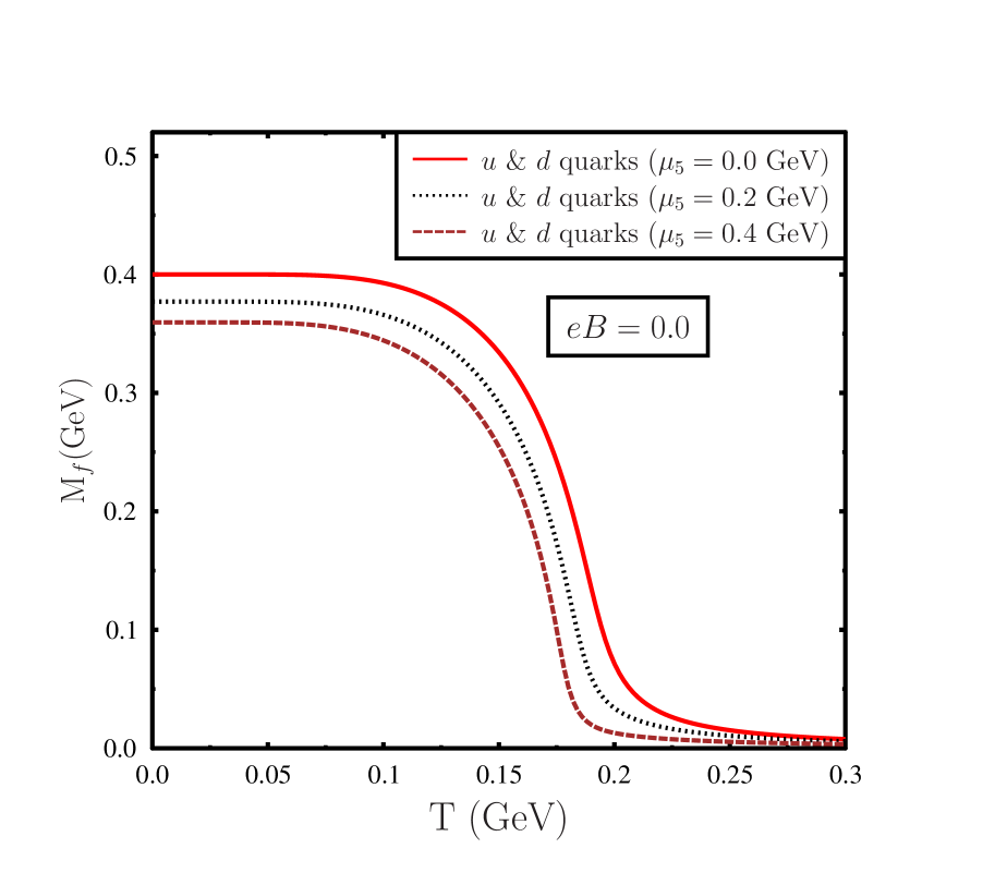
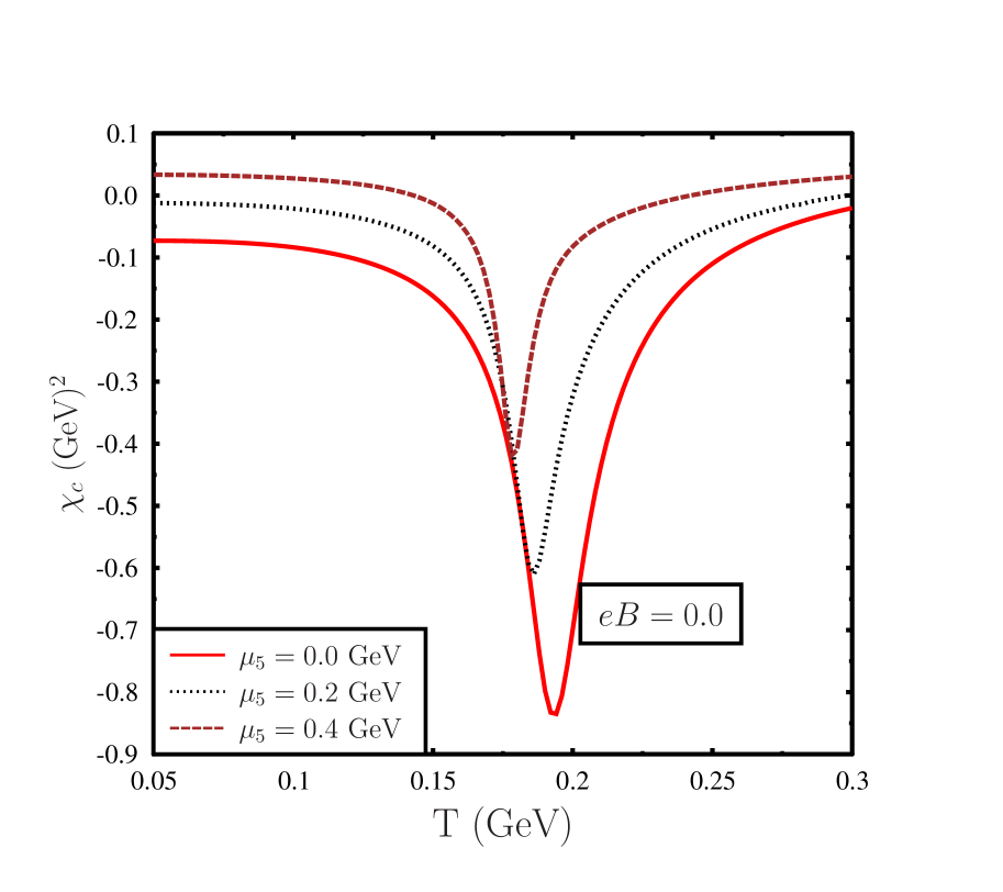
Figure 1: Left plot: Variation of constituent quark mass $M_{u}=M_{d}$ with temperature ($T$) for zero magnetic field but for various values of chiral chemical potential. Right plot: Variation of chiral susceptibility $\chi_{c}$ with temperature ($T$) for zero magnetic field but with different values of chiral chemical potential. Prominent peak in the chiral susceptibility plot shows the chiral transition temperature. From the left plot it is clear that with increasing chiral chemical potential ($\mu_{5}$) constituent mass decreases. From the susceptibility plot it is clear that transition temperature decreases with chiral chemical potential.

In Fig.(1) we show the variation of constituent quark masses and the associated chiral susceptibility as a function of temperature ($T$) for different values of chiral chemical potential ($\mu_{5}$) and for vanishing magnetic field. For zero magnetic field $\langle\bar{\psi}_{u}\psi_{u}\rangle=\langle\bar{\psi}_{d}\psi_{d}\rangle$, hence the masses of the $u$ and $d$ quarks remain same. From the left plot in Fig.(1) we can see that the constituent mass decreases with increasing chiral chemical potential. One can understand this result in the following way, chiral chemical potential is a conserved number of the associated chiral symmetry. Chiral symmetry is exact when the fermions are massless. Chiral symmetry try to protect the mass of the fermion from quantum corrections. Hence the chiral chemical potential which is the measure of the chiral symmetry tries to reduce the mass of the fermion. Right plot in Fig.(1) shows the chiral susceptibility for vanishing quark chemical potential and magnetic field. Peak in the chiral susceptibility plot shows the chiral transition temperature. Using Eq.(86) and Eq.(87) it can be shown that $\chi_{cu}=\chi_{cd}$ for vanishing magnetic field. Hence the variation of total chiral susceptibility ($\chi_{c}$) with temperature shows only one peak. However in the presence of magnetic field in general $\chi_{cu}$ can be different from $\chi_{cd}$ and variation of total chiral susceptibility $\chi_{c}$ with temperature can show multiple peaks. Results for non vanishing magnetic field will be shown later. From the right plot in Fig.(1) it is clear that with increasing chiral chemical potential ($\mu_{5}$) chiral transition temperature decreases.

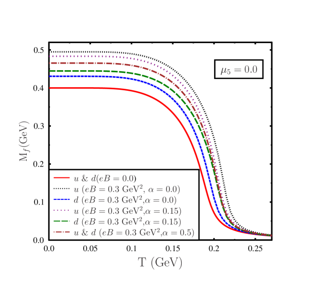
Figure 2: Variation of constituent quark masses $M_{u}$ and $M_{d}$ with temperature for vanishing chiral chemical potential but with finite magnetic field for different values of $\alpha$. For vanishing magnetic field $M_{u}$ and $M_{d}$ are same. Note that in the presence of magnetic field, for $\alpha=0.5$, although $\langle\bar{\psi}_{u}\psi_{u}\rangle\neq\langle\bar{\psi}_{d}\psi_{d}\rangle$, but the constituent quark masses $M_{u}=M_{d}$. However for $\alpha\neq 0.5$, the constituent quark masses $M_{u}\neq M_{d}$ in the presence of magnetic field.$\alpha=0.0$ corresponds to the case when there is no flavour mixing interaction, and $\alpha=0.5$ corresponds to maximal flavour mixing.

In Fig.(2) we show the variation of constituent quark masses $M_{u}$ and $M_{d}$ with temperature for vanishing chiral chemical potential and with finite magnetic field for different values of $\alpha$. From this figure it is clear that at non vanishing magnetic field constituent quark mass increases. At vanishing magnetic field constituent mass of $u$ and $d$ quarks are same. Although in the presence of magnetic field, quark condensates $\langle\bar{\psi}_{u}\psi_{u}\rangle\neq\langle\bar{\psi}_{d}\psi_{d}\rangle$, but for $\alpha=0.5$ the quark masses $M_{u}=M_{d}$. This is because for $\alpha=0.5$ constituent quark mass is $M_{f}=m-2g(\langle\bar{\psi}_{u}\psi_{u}\rangle+\langle\bar{\psi}_{d}\psi_{d}\rangle)$, as can be seen from Eq.(53). On the other hand for $\alpha\neq 0.5$ quark masses $M_{u}$ and $M_{d}$ are not the same. The difference between $M_{u}$ and $M_{d}$ increases with decrease in the value of $\alpha$ and this difference is largest when $\alpha=0.0$. $\alpha=0.0$ corresponds to the case when there is no flavour mixing interaction, and $\alpha=0.5$ corresponds to maximal flavour mixing. It is important to note that for vanishing magnetic field flavour mixing interaction does not affect the quark masses. Only in the presence of magnetic field when $\langle\bar{\psi}_{u}\psi_{u}\rangle\neq\langle\bar{\psi}_{d}\psi_{d}\rangle$, flavour mixing interaction affects the constituent quark masses $M_{u}$ and $M_{d}$ significantly.

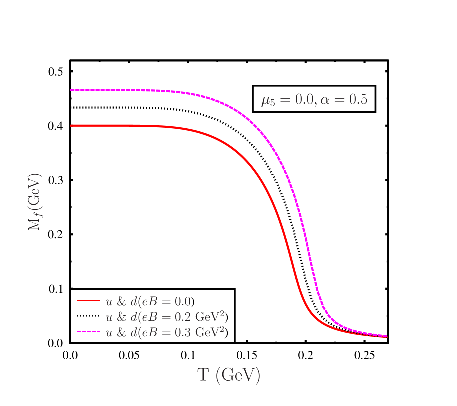
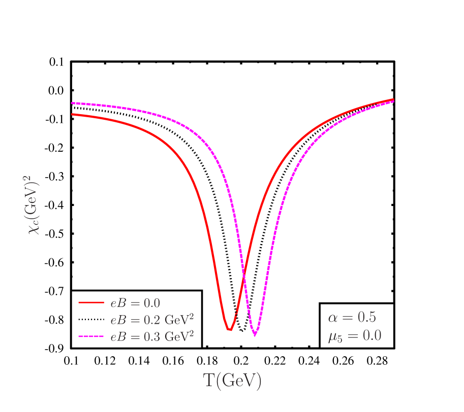
Figure 3: Left plot: variation of constituent quark mass $M_{u}$ and $M_{d}$, with temperature for vanishing chiral chemical potential, but with different values of magnetic field for $\alpha=0.5$. Right plot: Variation of chiral susceptibility $\chi_{c}$ with temperature ($T$) for vanishing chiral chemical potential, but with different values of magnetic field for $\alpha=0.5$. From the left plot it is clear that with increasing magnetic field constituent mass $M_{u}=M_{d}$ increases. From the susceptibility plot it is clear that transition temperature increases with magnetic field.

In Fig.(3) we show the variation of constituent quark masses $M_{u}$ and $M_{d}$ and the associated total chiral susceptibility, with temperature for vanishing chiral chemical potential and with different values of magnetic field for $\alpha=0.5$. It has been already mentioned that for $\alpha=0.5$ even in the presence of magnetic field $M_{u}=M_{d}$. From the left plot in Fig.(3) it is clear that with increasing magnetic field constituent quark mass increases. On the other hand from the right plot in Fig.(3) it is clear that chiral transition temperature increases with increasing magnetic field.

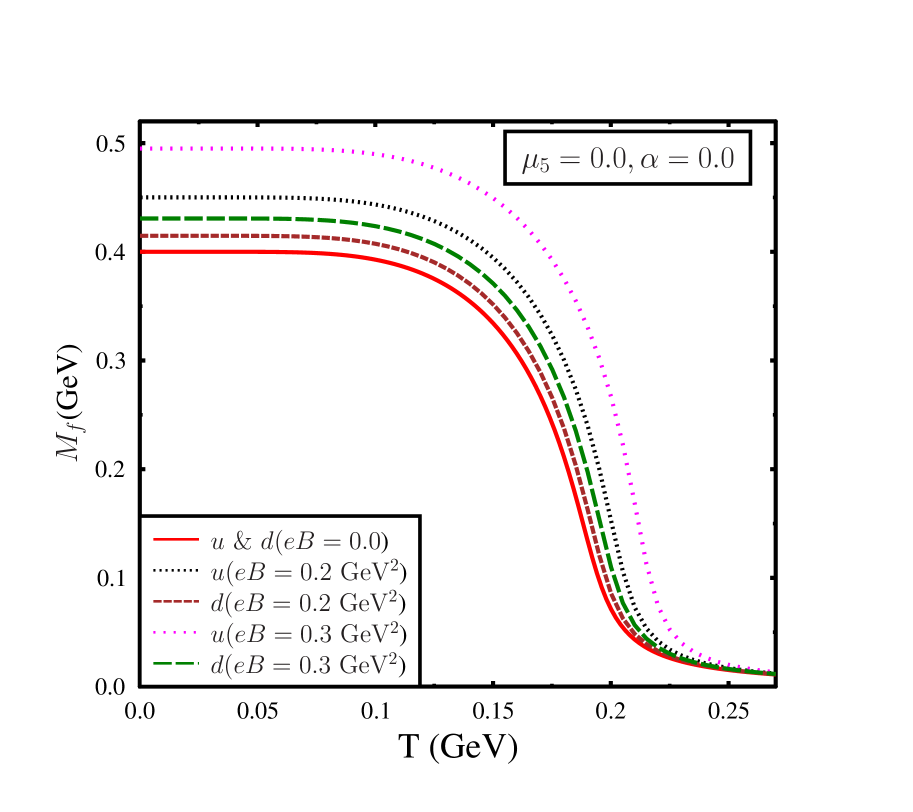
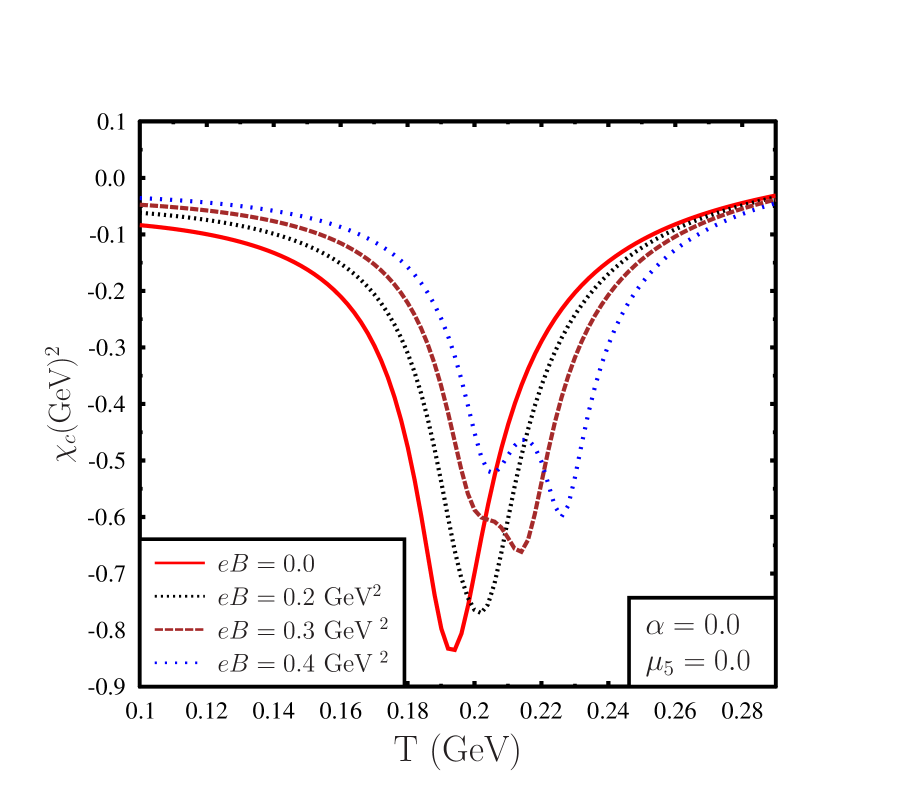
Figure 4: Left plot: variation of constituent quark mass $M_{u}$ and $M_{d}$, with temperature for vanishing chiral chemical potential, but with different values of magnetic field for $\alpha=0.0$. Right plot: Variation of chiral susceptibility $\chi_{c}$ with temperature ($T$) for vanishing chiral chemical potential, but with different values of magnetic field for $\alpha=0.5$. From the left plot it is clear that with increasing magnetic field constituent mass increases. From the susceptibility plot it is clear that transition temperature increases with magnetic field. In the right plot we can observe two distinct peaks at relatively large magnetic fields.

In Fig.(4) we show the variation of constituent quark masses $M_{u}$ and $M_{d}$ and the associated total chiral susceptibility, with temperature for vanishing chiral chemical potential and with different values of magnetic field for $\alpha=0.0$. For $\alpha=0.0$ there is no flavour mixing. From the left plot it is clear that at finite magnetic field $M_{u}\neq M_{d}$. This is because in the presence of magnetic field $u$ and $d$ quark condensates are different and in the absence of flavour mixing for $\alpha=0.0$, $M_{u}$ is independent of $\langle\bar{\psi}_{d}\psi_{d}\rangle$. Similarly $M_{d}$ is independent of $\langle\bar{\psi}_{u}\psi_{u}\rangle$ for $\alpha=0.0$. From the right plot in Fig.(4) it is clear that chiral transition temperature increases with increasing magnetic field. However it is important to mention that unlike the case when $\alpha=0.5$, in this case susceptibility plot shows two distinct peaks at relatively large magnetic field values. In fact these two peaks are associated with $u$ and $d$ quarks, which has been shown in Fig.(5). In the left plot of Fig.(5) we show $\chi_{cu}$, $\chi_{cd}$ and $\chi_{c}$ for $eB=0.4$GeV² and $\alpha=0.0$. On the other hand In the right plot of Fig.(5) we show $\chi_{cu}$, $\chi_{cd}$ and $\chi_{c}$ for $eB=0.4$GeV² and $\alpha=0.5$. From the left plot in Fig.(5) it is clear that for $\alpha=0.0$, i.e. in the absence of flavour mixing, at relatively large magnetic field chiral susceptibility $\chi_{c}$ shows two distinct peaks. These two peaks are associated with $u$ and $d$ quarks. At relatively large magnetic field with $\alpha=0.0$, chiral restoration of $d$ quark happens at relatively low temperature with respect to the $u$ quarks. This is due to the fact that at non zero magnetic field $M_{u}>M_{d}$, as can be seen in Fig.(4). On the other hand from the right plot in Fig.(5) we can see that, although $\langle\bar{\psi}_{u}\psi_{u}\rangle\neq\langle\bar{\psi}_{d}\psi_{d}\rangle$, $\chi_{cu}$ and $\chi_{cd}$ shows peak at same temperature. Hence for $\alpha=0.5$, at finite magnetic field chiral transition temperature for $u$ and $d$ quarks are same.

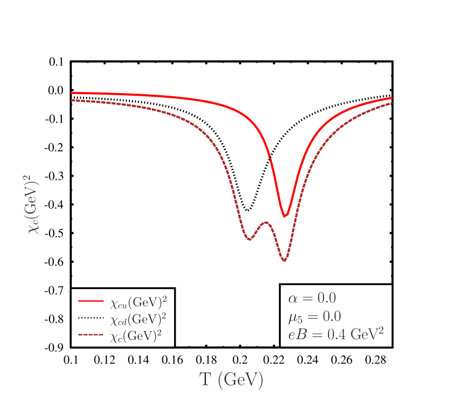
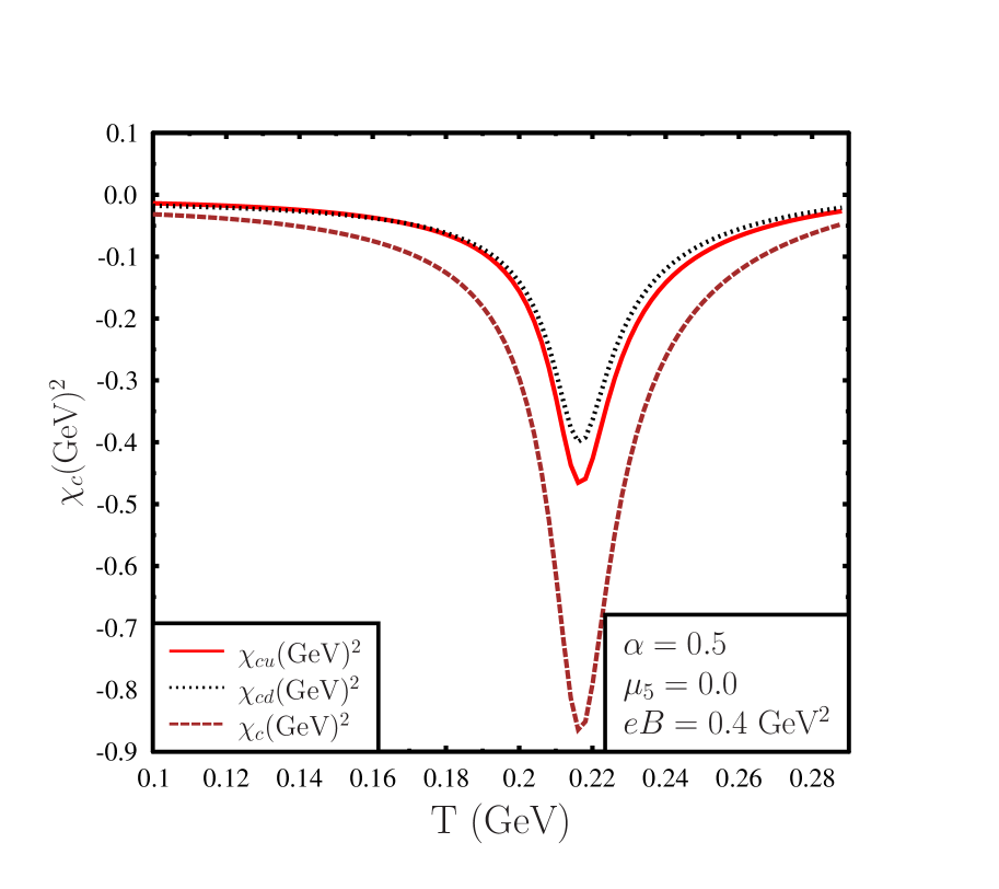
Figure 5: Left plot: Variation of $\chi_{cu}$, $\chi_{cd}$ and $\chi_{c}$ with temperature at vanishing chiral chemical potential, for $eB=0.4$GeV² and $\alpha=0.0$. Right plot: Variation of $\chi_{cu}$, $\chi_{cd}$ and $\chi_{c}$ with temperature at vanishing chiral chemical potential, for $eB=0.4$GeV² and $\alpha=0.5$. From the left plot it is clear that chiral susceptibility shows two distinct peaks at large magnetic field. This is due to the fact that at large magnetic field difference between $M_{u}$ and $M_{d}$ is large. On the other hand right plot shows that, for $\alpha=0.5$, $\langle\bar{\psi}_{u}\psi_{u}\rangle\neq\langle\bar{\psi}_{d}\psi_{d}\rangle$, $\chi_{cu}$ and $\chi_{cd}$ shows peak at same temperature. Hence for $\alpha=0.5$, at finite magnetic field chiral transition temperature for $u$ and $d$ quarks are same.

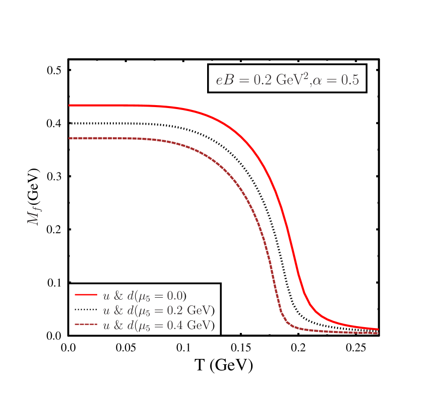
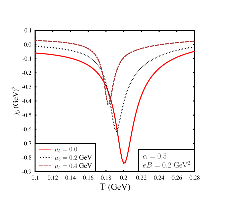
Figure 6: Left plot: Variation of constituent quark mass $M_{u}=M_{d}$, with temperature for finite magnetic field and finite chiral chemical potential. Right Plot: Variation of chiral susceptibility $\chi_{c}$ with temperature for finite magnetic field and finite chiral chemical potential. From this figure it is clear that with increasing chiral chemical potential quark mass as well as the chiral transition temperature decreases.

Finally in Fig.(6) we show the variation of quark constituent masses $M_{u}$ and $M_{d}$ and the associated susceptibilities with temperature for finite magnetic field and finite chiral chemical potential for $\alpha=0.5$. Behaviour of quark constituent masses and the chiral susceptibilities with temperature are similar for other values of $\alpha$. Left plot in Fig.(6) shows that with increasing value of chiral chemical potential and for finite magnetic field constituent quark mass decreases. This decrease in mass with increasing chiral chemical potential has also manifested in the right plot of Fig.(6), which shows that with increasing chiral chemical potential chiral transition temperature decreases.

VI conclusion

In this investigation we have studied chiral phase transition and the associated chiral susceptibility of the medium produced in ultra relativistic heavy ion collisions at vanishing quark chemical potential using Wigner function approach within the framework of two flavour NJL model. For a dynamical system like the medium produced in heavy ion collision quantum effects can be relevant. Hence the quantum kinetic equation is a suitable formalism to understand the evolution of these dynamical system. The central quantity of the quantum kinetic description is the Wigner function. Wigner function is the quantum mechanical analogue of classical distribution function. Different components of Wigner function satisfies quantum kinetic equation. However in this investigation we have restricted ourselves to the case of global equilibrium so that $T,\mu_{5}$ are constant and we do not consider evolution of Wigner function. In fact we could have done the analysis by estimating the mean field thermodynamic potential and minimizing the same to get the quark masses as well as the susceptibility.

We have looked into the behaviour of quark masses and chiral susceptibility within a two flavour NJL model with flavour mixing determinant interaction. In the absence of magnetic field $u$ and $d$ quark masses are degenerate, due to the isospin symmetry. However in the presence of magnetic field, due to different electric charge of $u$ and $d$ quark, constituent mass of $u$ and $d$ quark can be different. Our results show that while flavour mixing instanton induced interaction does not affect the quark masses in the absence of magnetic field, in the presence of magnetic field this interaction can affect quark masses. For maximal flavour mixing in NJL model for a non vanishing magnetic field $u$ and $d$ quark masses are degenerate. For non maximal flavour mixing quark masses are non degenerate in the presence of magnetic field. Constituent mass of $u$ and $d$ quark is larger for non vanishing magnetic field compared to $B=0$ counterpart. With increasing magnetic field constituent mass of $u$ and $d$ quark also increases. This apart, the chiral transition temperature is higher for non vanishing magnetic field with respect to the vanishing magnetic field case. This is the manifestation of magnetic catalysis i.e. in the presence of magnetic field the formation of chiral condensate is more probable, also the magnitude of the chiral condensate is higher for larger magnetic field. It is important to note that in the presence of non maximal flavour mixing instanton interaction , for vanishing magnetic field as well as for relatively small magnetic field the the chiral transition temperatures of $u$ and $d$ quark are same. But for larger magnetic field transition temperature of $u$ quark and $d$ quark are different. The difference between the transition temperature of $u$ and $d$ quark also increases with magnetic field. We have also shown that, non vanishing chiral chemical potential ($\mu_{5}$) reduces quark mass in the absence as well as in the presence of magnetic field. Unlike magnetic catalysis, with increasing chiral chemical potential ($\mu_{5}$), chiral transition temperature decreases. Also note that in presence of magnetic field, the chiral susceptibility shows a double peak structure due to isospin breaking in presence of magnetic field.

Appendix A Derivation of scalar condensate in a background magnetic field and chiral chemical potential

Scalar condensate in the terms of the scalar DHW function can be written as,

$$\langle\bar{\psi}\psi\rangle=\int d^{4}p\,F(p)$$ (101)

Using the explicit form of scalar DHW function ($F(p)$) as given in Eq.(43), scalar condensate in the presence of magnetic field as given in Eq.(101) can be expressed as,

$$\langle\bar{\psi}\psi\rangle =\int 2\pi p_{T}\,dp_{0}\,dp_{T}\,dp_{z}\,M\bigg{[}\sum_{n=0}^{\infty}V_{n}(p_{0},p_{z})\,\Lambda^{(n)}_{+}(p_{T})\,\,+\sum_{n=1}^{\infty}\frac{1}{\sqrt{p_{z}^{2}+2nqB}}\,A_{n}(p_{0},p_{z})p_{z}\,\Lambda^{(n)}_{-}(p_{T})\bigg{]}$$

$$=\int 2\pi p_{T}\,dp_{0}\,dp_{T}\,dp_{z}\,M\bigg{[}V_{0}(p_{0},p_{z})\,\Lambda^{(0)}_{+}(p_{T})\,+\sum_{n=1}^{\infty}V_{n}(p_{0},p_{z})\,\Lambda^{(n)}_{+}(p_{T})\,$$

$$~{}~{}~{}~{}~{}~{}~{}~{}~{}~{}~{}~{}~{}~{}~{}~{}~{}~{}~{}~{}~{}~{}~{}~{}~{}~{}~{}~{}~{}~{}~{}~{}~{}~{}~{}~{}~{}~{}~{}~{}~{}~{}~{}~{}~{}~{}~{}~{}~{}~{}~{}~{}~{}~{}~{}~{}~{}~{}~{}~{}~{}~{}+\sum_{n=1}^{\infty}\frac{1}{\sqrt{p_{z}^{2}+2nqB}}\,A_{n}(p_{0},p_{z})p_{z}\,\Lambda^{(n)}_{-}(p_{T})\bigg{]}$$

$$=\mathbb{I}_{1}+\mathbb{I}_{2}+\mathbb{I}_{3}$$ (102)

Now, the first term in Eq.(102),

$$\mathbb{I}_{1}=2\,\pi\,\iint dp_{0}\,dp_{z}\,MV_{0}(p_{0},p_{z})\,\,\int dp_{T}\,p_{T}\,\Lambda_{+}^{(0)}(p_{T}).$$ (103)

Using the explicit form of $V_{0}(p_{0},p_{z})$ and $\Lambda_{+}^{(0)}(p_{T})$, Eq.(103) can be expressed as,

$$\mathbb{I}_{1} =2\,\pi\,\iint dp_{0}\,dp_{z}\,\frac{2}{(2\pi)^{3}}\,M\delta\bigg{(}(p_{0}+\mu)^{2}-|E^{(0)}_{p_{z}}|^{2}\bigg{)}\,\bigg{[}\theta(p_{0}+\mu)\,f_{FD}(p_{0})\,$$

$$~{}~{}~{}~{}~{}~{}~{}~{}~{}~{}~{}~{}~{}~{}~{}~{}~{}~{}~{}~{}~{}~{}~{}~{}~{}+\theta(-p_{0}-\mu)\,[f_{FD}(-p_{0})-1]\bigg{]}\,\int dp_{T}\,p_{T}\,2\exp\left[{-p_{T}^{2}}/{qB}\right]$$

$$=\frac{qB}{(2\pi)^{2}}\int dp_{z}\,\frac{M}{E^{(0)}_{p_{z}}}\bigg{[}f_{FD}(E^{(0)}_{p_{z}}-\mu)\,+f_{FD}(E^{(0)}_{p_{z}}+\mu)-1\bigg{]}$$ (104)

The second term in Eq.(102),

$$\mathbb{I}_{2} =2\pi\sum_{n=1}^{\infty}\iint dp_{0}~{}dp_{z}~{}MV_{n}(p_{0},p_{z})\int dp_{T}p_{T}\Lambda_{+}^{(n)}(p_{T}).$$ (105)

Using the explicit form of $\Lambda_{+}^{(n)}(p_{T})$ one can calculate the following integral,

$$\int dp_{T}p_{T}\Lambda_{+}^{(n)}(p_{T}) =(-1)^{n}\int_{0}^{\infty}dp_{T}~{}p_{T}\bigg{[}L_{n}(2p_{T}^{2}/qB)-L_{n-1}(2p_{T}^{2}/qB)\bigg{]}\exp(-p_{T}^{2}/qB)=qB$$ (106)

To get the Eq.(106) we use the following identityhandbook ,

$$\int_{0}^{\infty}dx~{}\exp(-bx)L_{n}(x)=(b-1)^{n}b^{-n-1}.$$ (107)

Using Eq.(106) and the explicit form of $V_{n}(p_{0},p_{z})$, $\mathbb{I}_{2}$ can be written as,

$$\mathbb{I}_{2} =2\pi(qB)\iint~{}dp_{0}~{}dp_{z}\frac{2}{(2\pi)^{3}}M\sum_{s}\delta\left((p_{0}+\mu)^{2}-|E^{(n)}_{p_{z},s}|^{2}\right)\bigg{[}\theta(p_{0}+\mu)f_{FD}(p_{0})+\theta(-p_{0}-\mu)(f_{FD}(-p_{0})-1)\bigg{]}$$

$$=-\frac{qB}{(2\pi)^{2}}\sum_{n=1}^{\infty}\sum_{s}\int dp_{z}\frac{M}{E_{pz,s}^{(n)}}\bigg{[}1-f_{FD}(E^{(n)}_{p_{z},s}-\mu)-f_{FD}(E^{(n)}_{p_{z},s}+\mu)\bigg{]}$$ (108)

Now let us consider the third term of Eq.(102),

$$\mathbb{I}_{3}=2\,\pi\,\iint dp_{0}\,dp_{z}\,M\sum_{n=1}^{\infty}\frac{1}{\sqrt{p_{z}^{2}+2nqB}}\,A_{n}(p_{0},p_{z})\,p_{z}\,\,\int dp_{T}\,p_{T}\,\Lambda_{-}^{(n)}(p_{T}).$$ (109)

Using the explicit form of $\Lambda_{-}^{(n)}(p_{T})$, it can be shown that,

$$\int~{}dp_{T}~{}p_{T}\Lambda_{-}^{(n)}(p_{T}) =0$$ (110)

Hence the third term of the Eq.(102),

$$\mathbb{I}_{3}=0.$$ (111)

Hence using Eq.(104), Eq.(108) and Eq.(111), the scalar condensate is,

$$\langle\bar{\psi}\psi\rangle =-\frac{qB}{(2\pi)^{2}}\int dp_{z}\,\frac{M}{E^{(0)}_{p_{z}}}\bigg{[}1-f_{FD}(E^{(0)}_{p_{z}}-\mu)\,-f_{FD}(E^{(0)}_{p_{z}}+\mu)\bigg{]}\,$$

$$-\frac{qB}{(2\pi)^{2}}\sum_{n=1}^{\infty}\sum_{s}\int dp_{z}\,\frac{M}{E^{(n)}_{p_{z},s}}\bigg{[}1-f_{FD}(E^{(n)}_{p_{z},s}-\mu)-\,f_{FD}(E^{(n)}_{p_{z},s}+\mu)\bigg{]}.$$ (112)

Appendix B Regularization of chiral condensate in a background magnetic field

The scalar condensate of a quark of flavour $f$, with $N_{c}$ color degrees of freedom at finite temperature $(T)$, chemical potential ($\mu$) can be expressed as,

$$\langle\bar{\psi}_{f}\psi_{f}\rangle^{\mu_{5}=0}_{B\neq 0} =-\frac{N_{c}|q_{f}|B}{(2\pi)^{2}}\sum_{n=0}^{\infty}(2-\delta_{n,0})\int dp_{z}\,\frac{M_{0_{f}}}{\epsilon^{(n)}_{p_{z},f}}\Big{[}1-f_{FD}(\epsilon^{(n)}_{p_{z},f}-\mu)-\,f_{FD}(\epsilon^{(n)}_{p_{z},f}+\mu)\Big{]}\bigg{]}$$

$$=\langle\bar{\psi}_{f}\psi_{f}\rangle^{\mu_{5}=0}_{vac,B\neq 0}+\langle\bar{\psi}_{f}\psi_{f}\rangle^{\mu_{5}=0}_{med,B\neq 0},$$ (113)

where $\langle\bar{\psi}_{f}\psi_{f}\rangle^{\mu_{5}=0}_{vac,B\neq 0}$ is the $T=0,\mu=0$ part or the vacuum part of the scalar condensate and $\langle\bar{\psi}_{f}\psi_{f}\rangle^{\mu_{5}=0}_{med,B\neq 0}$ is the finite temperature and finite chemical potential part or the medium part of the scalar condensate in the presence of magnetic field. It is clear from the Eq.(113) the vacuum term is divergent for large momenta and however because of the distribution functions the medium part in Eq.(113) is not. Hence it is important to regulate the vacuum part in Eq.(113).

Let us consider the vacuum part $\langle\bar{\psi}_{f}\psi_{f}\rangle^{\mu_{5}=0}_{vac,B\neq 0}$ which is given as,

$$\langle\overline{\psi}_{f}\psi_{f}\rangle^{\mu_{5}=0}_{vac,B\neq 0} =-\frac{N_{c}}{2\pi}\sum_{n=0}^{\infty}(2-\delta_{n,0})|q_{f}|B\int_{-\infty}^{\infty}\frac{dp_{z}}{(2\pi)}\frac{M_{0_{f}}}{\epsilon_{p_{z},f}^{(n)}}$$

$$=-\frac{N_{c}}{2\pi}\sum_{n=0}^{\infty}2|q_{f}|B\int_{-\infty}^{\infty}\frac{dp_{z}}{(2\pi)}\frac{M_{0_{f}}}{\epsilon_{p_{z},f}^{(n)}}+\frac{N_{c}}{2\pi}|q_{f}|B\int_{-\infty}^{\infty}\frac{dp_{z}}{(2\pi)}\frac{M_{0_{f}}}{\epsilon_{p_{z},f}^{(0)}}$$

$$=\mathcal{I}_{1}+\mathcal{I}_{2}$$ (114)

Both integrals $\mathcal{I}_{1}$ and $\mathcal{I}_{2}$ are divergent at large momentum. These integrals can be regularized using dimensional regularization scheme. In this regularization scheme integral $\mathcal{I}_{1}$ can be expressed as,

$$\mathcal{I}_{1} =-\frac{N_{c}}{2\pi}\sum_{n=0}^{\infty}2|q_{f}|B\int_{-\infty}^{\infty}\frac{dp_{z}}{(2\pi)}\frac{M_{0_{f}}}{\epsilon_{p_{z},f}^{(n)}}$$

$$=-\frac{N_{c}}{2\pi}\sum_{n=0}^{\infty}2|q_{f}|B\frac{M_{0_{f}}\Gamma(\epsilon/2)}{(4\pi)^{(1-\epsilon)/2}\Gamma(1/2)(x_{0_{f}}+n)^{\epsilon/2}},$$ (115)

where the dimensionless variable $x_{0_{f}}\equiv M_{0_{f}}^{2}/2|q_{f}|B$. Similarly the integral $\mathcal{I}_{2}$ can be expressed as,

$$\mathcal{I}_{2} =\frac{N_{c}}{2\pi}|q_{f}|B\int\frac{dp_{z}}{(2\pi)}\frac{M_{0_{f}}}{\sqrt{M_{0_{f}}^{2}+p_{z}^{2}}}$$

$$=\frac{N_{c}M_{0_{f}}|q_{f}|B}{(2\pi)}\frac{\Gamma(\epsilon/2)}{(4\pi)^{(1-\epsilon)/2}\Gamma(1/2)x_{0_{f}}^{\epsilon/2}}$$ (116)

Using Eq.(115) and Eq.(116), vacuum part of the scalar condensate in the presence of magnetic field as given in Eq.(114), can be recasted as,

$$\mathcal{I}_{1}+\mathcal{I}_{2} =-\frac{N_{c}}{2\pi}2|q_{f}|BM_{0_{f}}\frac{\Gamma(\epsilon/2)}{(4\pi)^{(1-\epsilon)/2}\Gamma(1/2)}\bigg{[}\sum_{n=0}^{\infty}\frac{1}{(x_{0_{f}}+n)^{\epsilon/2}}-\frac{1}{2x_{0_{f}}^{\epsilon/2}}\bigg{]}$$

$$=-\frac{N_{c}}{2\pi}2|q_{f}|BM_{0_{f}}\frac{\Gamma(\epsilon/2)}{(4\pi)^{1/2}\Gamma(1/2)}\bigg{[}\zeta(\epsilon/2,x_{0_{f}})-\frac{1}{2x_{0_{f}}^{\epsilon/2}}\bigg{]}.$$ (117)

Expanding the right hand side of Eq.(117) around $\epsilon\rightarrow 0$ and keeping only the leading order terms, we get,

$$\mathcal{I}_{1}+\mathcal{I}_{2} =-\frac{N_{c}}{2\pi^{2}}|q_{f}|BM_{0_{f}}\bigg{[}-\frac{2x_{0_{f}}}{\epsilon}+\gamma_{E}x_{0_{f}}+\frac{1}{2}\ln x_{0_{f}}+\ln\Gamma(x_{0_{f}})-\frac{1}{2}\ln(2\pi)\bigg{]}$$ (118)

In Eq.(117), we have used the representation of Zeta function, which is given as zetafunction ,

$$\zeta(a,x)=\sum_{n=0}^{\infty}\frac{1}{(x+n)^{a}},$$ (119)

also, we have used the following identities to get Eq.(118),

$$\zeta(0,x)=(\frac{1}{2}-x),~{}~{}\text{and},~{}~{}\zeta^{\prime}(0,x)=\ln\Gamma(x)-\frac{1}{2}\ln(2\pi),~{}~{}\text{where}~{}~{}\zeta^{\prime}(0,x)=\frac{d\zeta(a,x)}{da}|_{a=0}$$ (120)

It is clear from Eq.(118), that the vacuum part has $1/\epsilon$ divergent part. To remove this $1/\epsilon$ divergence we use the following integral,

$$\mathcal{I}_{3}=-2N_{c}\int\frac{d^{3}p}{(2\pi)^{3}}\frac{M_{0_{f}}}{\sqrt{p^{2}+M_{0_{f}}^{2}}}$$ (121)

Using dimensional regularization method the integral in Eq.(121) can be recasted as,

$$\mathcal{I}_{3} =\frac{-2N_{c}M_{0_{f}}}{(4\pi)^{3/2}\Gamma(1/2)}\frac{\Gamma(-1+\epsilon/2)}{(2x_{0_{f}}|q_{f}|B)^{-1+\epsilon/2}}$$ (122)

Expand the right hand side of Eq.(122) around $\epsilon\rightarrow 0$ and keeping only the leading order terms we get,

$$\mathcal{I}_{3}=\frac{-N_{c}M_{0_{f}}|q_{f}|B}{2\pi^{2}}\bigg{[}-\frac{2x_{0_{f}}}{\epsilon}-x_{0_{f}}+x_{0_{f}}\gamma_{E}+x_{0_{f}}\ln x_{0_{f}}\bigg{]}$$ (123)

Using Eq.(118) and Eq.(123) we get,

$$\mathcal{I}_{1}+\mathcal{I}_{2}-\mathcal{I}_{3} =-\frac{N_{c}M_{0_{f}}|q_{f}|B}{2\pi^{2}}\bigg{[}x_{0_{f}}(1-\ln x_{0_{f}})+\ln\Gamma(x_{0_{f}})+\frac{1}{2}\ln\bigg{(}\frac{x_{0_{f}}}{2\pi}\bigg{)}\bigg{]}$$ (124)

Using Eq.(114) and Eq.(124), we have the regularized vacuum part of the scalar condensate in the presence of magnetic field and is given as,

$$\langle\overline{\psi}_{f}\psi_{f}\rangle^{\mu_{5}=0}_{vac,B\neq 0} =\mathcal{I}_{1}+\mathcal{I}_{2}-\mathcal{I}_{3}+\mathcal{I}_{3}$$

$$=-\frac{N_{c}M_{0_{f}}|q_{f}|B}{2\pi^{2}}\bigg{[}x_{0_{f}}(1-\ln x_{0_{f}})+\ln\Gamma(x_{0_{f}})+\frac{1}{2}\ln\bigg{(}\frac{x_{0_{f}}}{2\pi}\bigg{)}\bigg{]}-2N_{c}\int_{|\vec{p}|\leq\Lambda}\frac{d^{3}p}{(2\pi)^{3}}\frac{M_{0_{f}}}{\sqrt{p^{2}+M_{0_{f}}^{2}}}.$$ (125)

Again,

$$\mathcal{I}_{1} =\mathcal{I}_{1}-\mathcal{I}_{3}+\mathcal{I}_{3}$$

$$=-\frac{N_{c}|q_{f}|BM_{0_{f}}}{2\pi^{2}}\Bigg{[}\frac{1}{\epsilon}-\frac{\gamma_{E}}{2}+x_{0_{f}}(1-\ln x_{0_{f}})+\ln\Gamma(x_{0_{f}})-\frac{1}{2}\ln(2\pi)\Bigg{]}-2N_{c}\int\frac{d^{3}p}{(2\pi)^{3}}\frac{M_{0_{f}}}{\sqrt{p^{2}+M_{0_{f}}^{2}}}.$$ (126)

Hence,

$$\mathcal{I} \equiv-\frac{N_{c}|q_{f}|B}{(2\pi)^{2}}\sum_{s=\pm 1}\sum_{n=0}^{\infty}\int dp_{z}\frac{1}{\sqrt{p_{z}^{2}+M_{0_{f}}^{2}+2n|q_{f}|B}}$$

$$=-\frac{N_{c}}{2\pi^{2}}|q_{f}|B\Bigg{[}\frac{1}{\epsilon}-\frac{\gamma_{E}}{2}+x_{0_{f}}(1-\ln x_{0_{f}})+\ln\Gamma(x_{0_{f}})-\frac{1}{2}\ln(2\pi)\Bigg{]}-2N_{c}\int\frac{d^{3}p}{(2\pi)^{3}}\frac{1}{\sqrt{p^{2}+M_{0_{f}}^{2}}}$$ (127)

Using Eq.(127) we get,

$$\frac{N_{c}|q_{f}|B}{(2\pi)^{2}}\sum_{s=\pm 1}\sum_{n=0}^{\infty}\int dp_{z}\frac{1}{(p_{z}^{2}+M_{0_{f}}^{2}+2n|q_{f}|B)^{3/2}}\equiv\frac{1}{M_{0_{f}}}\frac{\partial\mathcal{I}}{\partial M_{0_{f}}}$$

$$=-\frac{N_{c}}{2\pi^{2}}\Bigg{[}-\ln x_{0_{f}}+\frac{\Gamma^{\prime}(x_{0_{f}})}{\Gamma(x_{0_{f}})}\Bigg{]}+2N_{c}\int_{|\vec{p}|\leq\Lambda}\frac{d^{3}p}{(2\pi)^{3}}\frac{1}{(p^{2}+M_{0_{f}}^{2})^{3/2}}$$ (128)

Appendix C Regularization of chiral condensate in a background magnetic field and chiral chemical potential

The scalar condensate of a quark of flavour $f$ with $N_{c}$ color degrees of freedom at finite temperature $(T)$, quark chemical potential ($\mu$), chiral chemical potential ($\mu_{5}$), electric charge ($q_{f}$) and magnetic field ($B$) can be expressed as,

$$\langle\bar{\psi}_{f}\psi_{f}\rangle^{\mu_{5}\neq 0}_{B\neq 0} =-\frac{N_{c}|q_{f}|B}{(2\pi)^{2}}\bigg{[}\int dp_{z}\,\frac{M_{f}}{E^{(0)}_{p_{z},f}}\Big{[}1-f_{FD}(E^{(0)}_{p_{z},f}-\mu)\,-f_{FD}(E^{(0)}_{p_{z},f}+\mu)\Big{]}\,$$

$$+\sum_{n=1}^{\infty}\sum_{s}\int dp_{z}\,\frac{M_{f}}{E^{(n)}_{p_{z},s,f}}\Big{[}1-f_{FD}(E^{(n)}_{p_{z},s,f}-\mu)-\,f_{FD}(E^{(n)}_{p_{z},s,f}+\mu)\Big{]}\bigg{]}$$

$$=\langle\bar{\psi}_{f}\psi_{f}\rangle^{\mu_{5}\neq 0}_{vac,B\neq 0}+\langle\bar{\psi}_{f}\psi_{f}\rangle^{\mu_{5}\neq 0}_{med,B\neq 0},$$ (129)

where $\langle\bar{\psi}_{f}\psi_{f}\rangle^{\mu_{5}\neq 0}_{vac,B\neq 0}$ is the $T=0,\mu=0$ part or the vacuum part of the scalar condensate and $\langle\bar{\psi}_{f}\psi_{f}\rangle^{\mu_{5}\neq 0}_{med,B\neq 0}$ is the finite temperature and finite chemical potential part or the medium part of the scalar condensate in the presence of magnetic field and chiral chemical potential ($\mu_{5}$). It is clear from the Eq.(129) that the vacuum term is divergent at large momenta and however because of the distribution functions the medium part in Eq.(129) is not. Hence the vacuum term has to be regularized.

The vacuum term in the presence of magnetic field and chiral chemical potential can be expressed as,

$$\langle\bar{\psi}_{f}\psi_{f}\rangle^{\mu_{5}\neq 0}_{vac,B\neq 0} =-N_{c}\frac{|q_{f}|B}{(2\pi)^{2}}\int dp_{z}\frac{M_{f}}{\sqrt{M_{f}^{2}+(p_{z}-\mu_{5})^{2}}}-N_{c}\frac{|q_{f}|B}{(2\pi)^{2}}\sum_{n=1}^{\infty}\sum_{s=\pm 1}\int dp_{z}\frac{M_{f}}{\sqrt{M_{f}^{2}+(\sqrt{p_{z}^{2}+2n|q_{f}|B}-s\mu_{5})^{2}}}$$

$$=-N_{c}\frac{|q_{f}|B}{(2\pi)^{2}}\sum_{n=0}^{\infty}\sum_{s=\pm 1}\int dp_{z}\frac{M_{f}}{\sqrt{M_{f}^{2}+(\sqrt{p_{z}^{2}+2n|q_{f}|B}-s\mu_{5})^{2}}}+N_{c}\frac{|q_{f}|B}{(2\pi)^{2}}\int dp_{z}\frac{M_{f}}{\sqrt{M_{f}^{2}+(p_{z}-\mu_{5})^{2}}}$$

$$=-N_{c}\frac{|q_{f}|B}{(2\pi)^{2}}\sum_{n=0}^{\infty}\sum_{s=\pm 1}\int dp_{z}\frac{1}{\pi}\int_{-\infty}^{\infty}dp_{4}\frac{M_{f}}{p_{4}^{2}+\left(M_{f}^{2}+(\sqrt{p_{z}^{2}+2n|q_{f}|B}-s\mu_{5})^{2}\right)}$$

$$~{}~{}~{}~{}~{}~{}~{}~{}~{}~{}~{}~{}~{}~{}~{}~{}~{}~{}~{}~{}+N_{c}\frac{|q_{f}|B}{(2\pi)^{2}}\int dp_{z}\frac{1}{\pi}\int_{-\infty}^{\infty}dp_{4}\frac{M_{f}}{p_{4}^{2}+M_{f}^{2}+(p_{z}-\mu_{5})^{2}}$$

$$=I_{1}+I_{2}$$ (130)

Using the regularization method discussed in Ref.chiralNJL7 we can write the integrand of the integral $I_{1}$ as given in the Eq.(130) as following

$$\frac{1}{p_{4}^{2}+M_{f}^{2}+(\sqrt{p_{z}^{2}+2n|q_{f}|B}-s\mu_{5})^{2}}$$

$$=\frac{1}{p_{4}^{2}+p_{z}^{2}+M_{0_{f}}^{2}+2n|q_{f}|B}-\frac{1}{p_{4}^{2}+p_{z}^{2}+M_{0_{f}}^{2}+2n|q_{f}|B}+\frac{1}{p_{4}^{2}+M_{f}^{2}+(\sqrt{p_{z}^{2}+2n|q_{f}|B}-s\mu_{5})^{2}}$$

$$=\frac{1}{p_{4}^{2}+p_{z}^{2}+M_{0_{f}}^{2}+2n|q_{f}|B}+\frac{M_{0_{f}}^{2}-M_{f}^{2}-\mu_{5}^{2}+2s\mu_{5}\sqrt{p_{z}^{2}+2n|q_{f}|B}}{\bigg{(}p_{4}^{2}+p_{z}^{2}+M_{0_{f}}^{2}+2n|q_{f}|B\bigg{)}\bigg{(}p_{4}^{2}+M_{f}^{2}+(\sqrt{p_{z}^{2}+2n|q_{f}|B}-s\mu_{5})^{2}\bigg{)}}$$ (131)

Using Eq.(131) twice we can write the integrand of the integral $I_{1}$ in the following way,

$$\frac{1}{p_{4}^{2}+M_{f}^{2}+(\sqrt{p_{z}^{2}+2n|q_{f}|B}-s\mu_{5})^{2}}=\frac{1}{p_{4}^{2}+p_{z}^{2}+M_{0_{f}}^{2}+2n|q_{f}|B}+\frac{A+2s\mu_{5}\sqrt{p_{z}^{2}+2n|q_{f}|B}}{\bigg{(}p_{4}^{2}+p_{z}^{2}+M_{0_{f}}^{2}+2n|q_{f}|B\bigg{)}^{2}}$$

$$~{}~{}~{}~{}~{}~{}~{}~{}~{}~{}~{}~{}+\frac{(A+2s\mu_{5}\sqrt{p_{z}^{2}+2n|q_{f}|B})^{2}}{\bigg{(}p_{4}^{2}+p_{z}^{2}+M_{0_{f}}^{2}+2n|q_{f}|B\bigg{)}^{3}}+\frac{(A+2s\mu_{5}\sqrt{p_{z}^{2}+2n|q_{f}|B})^{3}}{\bigg{(}p_{4}^{2}+p_{z}^{2}+M_{0_{f}}^{2}+2n|q_{f}|B\bigg{)}^{3}\bigg{(}p_{4}^{2}+M_{f}^{2}+(\sqrt{p_{z}^{2}+2n|q_{f}|B}-s\mu_{5})^{2}\bigg{)}},$$ (132)

where $A=M_{0_{f}}^{2}-M_{f}^{2}-\mu_{5}^{2}$. Performing $p_{4}$ integration in each term of Eq.(132) we get,

$$\frac{1}{\pi}\sum_{s}\int dp_{4}\frac{1}{p_{4}^{2}+p_{z}^{2}+M_{0_{f}}^{2}+2n|q_{f}|B}=\sum_{s}\frac{1}{\sqrt{p_{z}^{2}+M_{0_{f}}^{2}+2n|q_{f}|B}}$$ (133)

$$\frac{1}{\pi}\sum_{s}\int dp_{4}\frac{A+2s\mu_{5}\sqrt{p_{z}^{2}+2n|q_{f}|B}}{\bigg{(}p_{4}^{2}+p_{z}^{2}+M_{0_{f}}^{2}+2n|q_{f}|B\bigg{)}^{2}} =\sum_{s}\frac{1}{2}\frac{A}{\bigg{(}p_{z}^{2}+M_{0_{f}}^{2}+2n|q_{f}|B\bigg{)}^{3/2}}$$ (134)

$$\frac{1}{\pi}\sum_{s}\int dp_{4}\frac{(A+2s\mu_{5}\sqrt{p_{z}^{2}+2n|q_{f}|B})^{2}}{\bigg{(}p_{4}^{2}+p_{z}^{2}+M_{0_{f}}^{2}+2n|q_{f}|B\bigg{)}^{3}}=\sum_{s}\Bigg{[}\frac{3}{8}\frac{A^{2}}{(p_{z}^{2}+M_{0_{f}}^{2}+2n|q_{f}|B)^{5/2}}-\frac{3}{2}\frac{\mu_{5}^{2}M_{0_{f}}^{2}}{(p_{z}^{2}+M_{0_{f}}^{2}+2n|q_{f}|B)^{5/2}}$$

$$~{}~{}~{}~{}~{}~{}~{}~{}~{}~{}~{}~{}~{}~{}~{}~{}~{}~{}~{}~{}~{}~{}~{}~{}~{}~{}~{}~{}~{}~{}~{}~{}~{}~{}~{}~{}~{}~{}~{}~{}~{}~{}~{}~{}~{}~{}~{}~{}~{}~{}~{}~{}~{}~{}~{}~{}~{}~{}~{}~{}~{}~{}~{}+\frac{3}{2}\frac{\mu_{5}^{2}}{(p_{z}^{2}+M_{0_{f}}^{2}+2n|q_{f}|B)^{3/2}}\Bigg{]}$$ (135)

$$\frac{1}{\pi}\sum_{s}\int dp_{4}\frac{(A+2s\mu_{5}\sqrt{p_{z}^{2}+2n|q_{f}|B})^{3}}{\bigg{(}p_{4}^{2}+p_{z}^{2}+M_{0_{f}}^{2}+2n|q_{f}|B\bigg{)}^{3}\bigg{(}p_{4}^{2}+M_{f}^{2}+(\sqrt{p_{z}^{2}+2n|q_{f}|B}-s\mu_{5})^{2}\bigg{)}}$$

$$=\frac{1}{\pi}\sum_{s}\int dp_{4}\int_{0}^{1}dx\frac{3(1-x)^{2}(A+2s\mu_{5}\sqrt{p_{z}^{2}+2n|q_{f}|B})^{3}}{\Bigg{[}x\bigg{(}p_{4}^{2}+M_{f}^{2}+(\sqrt{p_{z}^{2}+2n|q_{f}|B}-s\mu_{5})^{2}\bigg{)}+(1-x)\bigg{(}p_{4}^{2}+p_{z}^{2}+M_{0_{f}}^{2}+2n|q_{f}|B\bigg{)}\Bigg{]}^{4}}$$

$$=\sum_{s}\frac{15}{16}\int_{0}^{1}dx\frac{(1-x)^{2}(A+2s\mu_{5}\sqrt{p_{z}^{2}+2n|q_{f}|B})^{3}}{\Bigg{[}p_{z}^{2}+M_{0_{f}}^{2}+2n|q_{f}|B-x(A+2s\mu_{5}\sqrt{p_{z}^{2}+2n|q_{f}|B})\Bigg{]}^{7/2}}$$ (136)

Using Eq.(133),Eq.(134),Eq.(135) and Eq.(136), integral $I_{1}$ in Eq.(130) can be expressed as,

$$I_{1} =-N_{c}\frac{|q_{f}|B}{(2\pi)^{2}}\sum_{n=0}^{\infty}\sum_{s=\pm 1}\int dp_{z}\frac{M_{f}}{\sqrt{M_{f}^{2}+(\sqrt{p_{z}^{2}+2n|q_{f}|B}-s\mu_{5})^{2}}}$$

$$=I_{1_{\text{quad}}}-\frac{M_{f}(M_{0_{f}}^{2}-M_{f}^{2}+2\mu_{5}^{2})}{2}I_{1_{\text{log}}}+I_{1_{\text{finite1}}}+I_{1_{\text{finite2}}},$$ (137)

where

$$I_{1_{\text{quad}}}=-N_{c}\frac{|q_{f}|B}{(2\pi)^{2}}\sum_{n=0}^{\infty}\sum_{s=\pm 1}\int dp_{z}\frac{M_{f}}{\sqrt{p_{z}^{2}+M_{0_{f}}^{2}+2n|q_{f}|B}},$$ (138)

$$I_{1_{\text{log}}}=N_{c}\frac{|q_{f}|B}{(2\pi)^{2}}\sum_{n=0}^{\infty}\sum_{s=\pm 1}\int dp_{z}\frac{1}{(p_{z}^{2}+M_{0_{f}}^{2}+2n|q_{f}|B)^{3/2}},$$ (139)

$$I_{1_{\text{finite1}}}=-N_{c}\frac{|q_{f}|B}{(2\pi)^{2}}\sum_{n=0}^{\infty}\sum_{s=\pm 1}\int dp_{z}\left(\frac{3}{8}\right)\Bigg{[}\frac{M_{f}A^{2}-4M_{f}M_{0_{f}}^{2}\mu_{5}^{2}}{(p_{z}^{2}+M_{0_{f}}^{2}+2n|q_{f}|B)^{5/2}}\Bigg{]},$$ (140)

$$I_{1_{\text{finite2}}}=-N_{c}\frac{|q_{f}|B}{(2\pi)^{2}}\left(\frac{15}{16}\right)\sum_{n=0}^{\infty}\sum_{s=\pm 1}\int dp_{z}\int_{0}^{1}dx\frac{(1-x)^{2}M_{f}(A+2s\mu_{5}\sqrt{p_{z}^{2}+2n|q_{f}|B})^{3}}{\Bigg{[}p_{z}^{2}+M_{0_{f}}^{2}+2n|q_{f}|B-x(A+2s\mu_{5}\sqrt{p_{z}^{2}+2n|q_{f}|B})\Bigg{]}^{7/2}}.$$ (141)

In a similar way the integral $I_{2}$ in Eq.(130) can also be written as,

$$I_{2} =N_{c}\frac{|q_{f}|B}{(2\pi)^{2}}\int dp_{z}\frac{M_{f}}{\sqrt{M_{f}^{2}+(p_{z}-\mu_{5})^{2}}}$$

$$=N_{c}\frac{|q_{f}|B}{(2\pi)^{2}}\int dp_{z}\frac{M_{f}}{\sqrt{M_{f}^{2}+(p_{z}-\mu_{5})^{2}}}-N_{c}\frac{|q_{f}|B}{(2\pi)^{2}}\int dp_{z}\frac{M_{f}}{\sqrt{p_{z}^{2}+M_{0_{f}}^{2}}}+N_{c}\frac{|q_{f}|B}{(2\pi)^{2}}\int dp_{z}\frac{M_{f}}{\sqrt{p_{z}^{2}+M_{0_{f}}^{2}}}$$

$$=\left(\frac{1}{2}\right)N_{c}\frac{|q_{f}|B}{(2\pi)^{2}}\int dp_{z}\int_{0}^{1}dx\frac{M_{f}\bigg{(}A+2p_{z}\mu_{5}\bigg{)}}{\Bigg{[}p_{z}^{2}+M_{0_{f}}^{2}-x\bigg{(}A+2p_{z}\mu_{5}\bigg{)}\Bigg{]}^{3/2}}+N_{c}\frac{|q_{f}|B}{(2\pi)^{2}}\int dp_{z}\frac{M_{f}}{\sqrt{p_{z}^{2}+M_{0_{f}}^{2}}}$$

$$=I_{2_{\text{finite}}}+I_{2_{\text{log}}}$$ (142)

Using Eq.(137) and Eq.(142), Eq.(130) can be recasted as,

$$\langle\bar{\psi}_{f}\psi_{f}\rangle^{\mu_{5}\neq 0}_{vac,B\neq 0}=-\frac{M_{f}(M_{0_{f}}^{2}-M_{f}^{2}+2\mu_{5}^{2})}{2}I_{1_{\text{log}}}+I_{1_{\text{finite1}}}+I_{1_{\text{finite2}}}+I_{2_{\text{finite}}}+I_{1_{\text{quad}}}+I_{2_{\text{log}}},$$ (143)

where

$$I_{1_{\text{log}}}=-\frac{N_{c}}{2\pi^{2}}\Bigg{[}-\ln x_{0_{f}}+\frac{\Gamma^{\prime}(x_{0_{f}})}{\Gamma(x_{0_{f}})}\Bigg{]}+2N_{c}\int_{|\vec{p}|\leq\Lambda}\frac{d^{3}p}{(2\pi)^{3}}\frac{1}{(p^{2}+M_{0_{f}}^{2})^{3/2}},$$ (144)

and

$$I_{1_{\text{quad}}}+I_{2_{\text{log}}} =-\frac{N_{c}M_{f}|q_{f}|B}{2\pi^{2}}\bigg{[}x_{0_{f}}(1-\ln x_{0_{f}})+\ln\Gamma(x_{0_{f}})+\frac{1}{2}\ln\bigg{(}\frac{x_{0_{f}}}{2\pi}\bigg{)}\bigg{]}-2N_{c}\int_{|\vec{p}|\leq\Lambda}\frac{d^{3}p}{(2\pi)^{3}}\frac{M_{f}}{\sqrt{p^{2}+M_{0_{f}}^{2}}}.$$ (145)

In Eq.(144) and (145) we have used (128) and (125) respectively.

Appendix D Chiral susceptibility and its regularization in the presence of a background magnetic field and chiral chemical potential

Using Eq.(130), we get,

$$\frac{\partial\langle\bar{\psi}_{f}\psi_{f}\rangle^{\mu_{5}\neq 0}_{vac,B\neq 0}}{\partial M_{f}} =-\frac{N_{c}|q_{f}|B}{(2\pi)^{2}}\sum_{n=0}^{\infty}\sum_{s=\pm 1}\int dp_{z}\frac{1}{\sqrt{M_{f}^{2}+(\sqrt{p_{z}^{2}+2n|q_{f}|B}-s\mu_{5})^{2}}}+\frac{N_{c}|q_{f}|B}{(2\pi)^{2}}\int dp_{z}\frac{1}{\sqrt{M_{f}^{2}+(p_{z}-\mu_{5})^{2}}}$$

$$+\frac{N_{c}|q_{f}|B}{(2\pi)^{2}}\sum_{n=0}^{\infty}\sum_{s=\pm 1}\int dp_{z}\frac{M_{f}^{2}}{\left(M_{f}^{2}+(\sqrt{p_{z}^{2}+2n|q_{f}|B}-s\mu_{5})^{2}\right)^{3/2}}-\frac{N_{c}|q_{f}|B}{(2\pi)^{2}}\int dp_{z}\frac{M_{f}^{2}}{\left(M_{f}^{2}+(p_{z}-\mu_{5})^{2}\right)^{3/2}}$$

$$=\mathbf{I}_{1}+\mathbf{I}_{2}+\mathbf{I}_{3}+\mathbf{I}_{4}$$ (146)

Using Eq.(137), we can write,

$$\mathbf{I}_{1}= -N_{c}\frac{|q_{f}|B}{(2\pi)^{2}}\sum_{n=0}^{\infty}\sum_{s=\pm 1}\int dp_{z}\frac{1}{\sqrt{M_{f}^{2}+(\sqrt{p_{z}^{2}+2n|q_{f}|B}-s\mu_{5})^{2}}}$$

$$=\mathbf{I}_{1,\text{quad}}-\frac{(M_{0_{f}}^{2}-M_{f}^{2}+2\mu_{5}^{2})}{2}\mathbf{I}_{1,\text{log}}+\mathbf{I}_{1,\text{finite1}}+\mathbf{I}_{1,\text{finite2}},$$ (147)

where

$$\mathbf{I}_{1,\text{quad}}=-N_{c}\frac{|q_{f}|B}{(2\pi)^{2}}\sum_{n=0}^{\infty}\sum_{s=\pm 1}\int dp_{z}\frac{1}{\sqrt{p_{z}^{2}+M_{0_{f}}^{2}+2n|q_{f}|B}},$$ (148)

$$\mathbf{I}_{1,\text{log}}=N_{c}\frac{|q_{f}|B}{(2\pi)^{2}}\sum_{n=0}^{\infty}\sum_{s=\pm 1}\int dp_{z}\frac{1}{(p_{z}^{2}+M_{0_{f}}^{2}+2n|q_{f}|B)^{3/2}},$$ (149)

$$\mathbf{I}_{1,\text{finite1}}=-N_{c}\frac{|q_{f}|B}{(2\pi)^{2}}\sum_{n=0}^{\infty}\sum_{s=\pm 1}\int dp_{z}\bigg{(}\frac{3}{8}\bigg{)}\Bigg{[}\frac{A^{2}-4M_{0_{f}}^{2}\mu_{5}^{2}}{(p_{z}^{2}+M_{0_{f}}^{2}+2n|q_{f}|B)^{5/2}}\Bigg{]},$$ (150)

$$\mathbf{I}_{1,\text{finite2}}=-N_{c}\frac{|q_{f}|B}{(2\pi)^{2}}\left(\frac{15}{16}\right)\sum_{n=0}^{\infty}\sum_{s=\pm 1}\int dp_{z}\int_{0}^{1}dx\frac{(1-x)^{2}(A+2s\mu_{5}\sqrt{p_{z}^{2}+2n|q_{f}|B})^{3}}{\Bigg{[}p_{z}^{2}+M_{0_{f}}^{2}+2n|q_{f}|B-x(A+2s\mu_{5}\sqrt{p_{z}^{2}+2n|q_{f}|B})\Bigg{]}^{7/2}}.$$ (151)

The integral $\mathbf{I}_{2}$ in Eq.(146) can be expressed as,

$$\mathbf{I}_{2} =N_{c}\frac{|q_{f}|B}{(2\pi)^{2}}\int dp_{z}\frac{1}{\sqrt{M_{f}^{2}+(p_{z}-\mu_{5})^{2}}}=\mathbf{I}_{2,\text{finite}}+\mathbf{I}_{2,\text{log}},$$ (152)

where divergence free $\mathbf{I}_{2,\text{finite}}$ is,

$$\mathbf{I}_{2,\text{finite}}=\left(\frac{1}{2}\right)N_{c}\frac{|q_{f}|B}{(2\pi)^{2}}\int dp_{z}\int_{0}^{1}dx\frac{\bigg{(}A+2p_{z}\mu_{5}\bigg{)}}{\Bigg{[}p_{z}^{2}+M_{0_{f}}^{2}-x\bigg{(}A+2p_{z}\mu_{5}\bigg{)}\Bigg{]}^{3/2}},$$ (153)

and the divergence term $\mathbf{I}_{2,\text{log}}$ is,

$$\mathbf{I}_{2,\text{log}}=\frac{N_{c}|q_{f}|B}{(2\pi)^{2}}\int dp_{z}\frac{1}{\sqrt{p_{z}^{2}+M_{0_{f}}^{2}}}.$$ (154)

Similarly, the integral $\mathbf{I}_{3}$ can be separated into a divergent and a convergent terms as,

$$\mathbf{I}_{3} =\frac{N_{c}|q_{f}|B}{(2\pi)^{2}}\sum_{n=0}^{\infty}\sum_{s=\pm 1}\int dp_{z}\frac{M_{f}^{2}}{\left(M_{f}^{2}+(\sqrt{p_{z}^{2}+2n|q_{f}|B}-s\mu_{5})^{2}\right)^{3/2}}=\mathbf{I}_{3,\text{finite}}+\mathbf{I}_{3,\text{log}},$$ (155)

where

$$\mathbf{I}_{3,\text{finite}}=\frac{N_{c}|q_{f}|B}{(2\pi)^{2}}\sum_{n=0}^{\infty}\sum_{s=\pm 1}\int dp_{z}M_{f}^{2}\Bigg{[}\frac{1}{\left(M_{f}^{2}+(\sqrt{p_{z}^{2}+2n|q_{f}|B}-s\mu_{5})^{2}\right)^{3/2}}-\frac{1}{\left(M_{0_{f}}^{2}+p_{z}^{2}+2n|q_{f}|B\right)^{3/2}}\Bigg{]},$$ (156)

and

$$\mathbf{I}_{3,\text{log}}=\frac{N_{c}|q_{f}|B}{(2\pi)^{2}}\sum_{n=0}^{\infty}\sum_{s=\pm 1}\int dp_{z}\frac{M_{f}^{2}}{\left(M_{0_{f}}^{2}+p_{z}^{2}+2n|q_{f}|B\right)^{3/2}}.$$ (157)

It can be shown that the term $\mathbf{I}_{3,\text{finite}}$ is finite. On the other hand the term $\mathbf{I}_{3,\text{log}}$ is not convergent at large momenta. Using Eq.(147), Eq.(152) and Eq.(155), Eq.(146) can be rearranged in the following way,

$$\frac{\partial\langle\bar{\psi}_{f}\psi_{f}\rangle^{\mu_{5}\neq 0}_{vac,B\neq 0}}{\partial M_{f}} =\mathbf{I}_{1,\text{quad}}-\frac{M_{0_{f}}^{2}-M_{f}^{2}+2\mu_{5}^{2}}{2}\mathbf{I}_{1,\text{log}}+\mathbf{I}_{1,\text{finite1}}+\mathbf{I}_{1,\text{finite2}}+\mathbf{I}_{2,\text{finite}}+\mathbf{I}_{3,\text{finite}}$$

$$~{}~{}~{}~{}~{}~{}~{}~{}~{}~{}~{}~{}~{}~{}~{}~{}~{}~{}~{}~{}+\mathbf{I}_{4}+\mathbf{I}_{2,\text{log}}+\mathbf{I}_{3,\text{log}}$$

$$=-\frac{M_{0_{f}}^{2}-M_{f}^{2}+2\mu_{5}^{2}}{2}\mathbf{I}_{1,\text{log}}+\mathbf{I}_{1,\text{finite1}}+\mathbf{I}_{1,\text{finite2}}+\mathbf{I}_{2,\text{finite}}+\mathbf{I}_{3,\text{finite}}$$

$$+\bigg{(}\mathbf{I}_{4}+\frac{N_{c}|q_{f}|B}{(2\pi)^{2}}\int dp_{z}\frac{M_{f}^{2}}{(M_{0_{f}}^{2}+p_{z}^{2})^{3/2}}\bigg{)}+(\mathbf{I}_{1,\text{quad}}+\mathbf{I}_{2,\text{log}})$$

$$+\bigg{(}\mathbf{I}_{3,\text{log}}-\frac{N_{c}|q_{f}|B}{(2\pi)^{2}}\int dp_{z}\frac{M_{f}^{2}}{(M_{0_{f}}^{2}+p_{z}^{2})^{3/2}}\bigg{)}$$

$$=-\frac{M_{0_{f}}^{2}-M_{f}^{2}+2\mu_{5}^{2}}{2}\mathbf{I}_{1,\text{log}}+\mathbf{I}_{1,\text{finite1}}+\mathbf{I}_{1,\text{finite2}}+\mathbf{I}_{2,\text{finite}}+\mathbf{I}_{3,\text{finite}}+\mathbf{I}_{\text{finite}}+\mathbf{I}_{\text{quad}}+\mathbf{I}_{\text{log}},$$ (158)

where $\mathbf{I}_{\text{finite}}$ is,

$$\mathbf{I}_{\text{finite}}=\mathbf{I}_{4}+\frac{N_{c}|q_{f}|B}{(2\pi)^{2}}\int dp_{z}\frac{M_{f}^{2}}{(p^{2}+M_{0_{f}}^{2})^{3/2}},$$ (159)

and

$$\mathbf{I}_{\text{quad}} =\mathbf{I}_{1,\text{quad}}+\mathbf{I}_{2,\text{log}}$$

$$=-\frac{N_{c}|q_{f}|B}{2\pi^{2}}\Bigg{[}x_{0_{f}}(1-\ln x_{0_{f}})+\ln\Gamma(x_{0_{f}})+\frac{1}{2}\ln\left(\frac{x_{0_{f}}}{2\pi}\right)\Bigg{]}-\frac{2N_{c}}{(2\pi)^{3}}\int_{|\vec{p}|\leq\Lambda}d^{3}p\frac{1}{\sqrt{p^{2}+M_{0_{f}}^{2}}}.$$ (160)

$$\mathbf{I}_{\text{log}} =\mathbf{I}_{3,\text{log}}-\frac{N_{c}|q_{f}|B}{(2\pi)^{2}}\int dp_{z}\frac{M_{f}^{2}}{(p^{2}+M_{0_{f}}^{2})^{3/2}},$$

$$=-\frac{N_{c}M_{f}^{2}}{2\pi^{2}}\Bigg{[}-\ln x_{0_{f}}+\frac{1}{2x_{0_{f}}}+\frac{\Gamma^{\prime}(x_{0_{f}})}{\Gamma(x_{0_{f}})}\Bigg{]}+\frac{2N_{c}}{(2\pi)^{3}}\int_{|\vec{p}|\leq\Lambda}d^{3}p\frac{M_{f}^{2}}{\left(p^{2}+M_{0_{f}}\right)^{3/2}},$$ (161)

with,

$$\mathbf{I}_{1,\text{log}}=\frac{N_{c}|q_{f}|B}{(2\pi)^{2}}\sum_{s=\pm 1}\sum_{n=0}^{\infty}\int dp_{z}\frac{1}{(p_{z}^{2}+M_{0_{f}}^{2}+2n|q_{f}|B)^{3/2}} =-\frac{N_{c}}{2\pi^{2}}\Bigg{[}-\ln x_{0_{f}}+\frac{\Gamma^{\prime}(x_{0_{f}})}{\Gamma(x_{0_{f}})}\Bigg{]}$$

$$~{}~{}~{}~{}~{}~{}~{}+2N_{c}\int_{|\vec{p}|\leq\Lambda}\frac{d^{3}p}{(2\pi)^{3}}\frac{1}{(p^{2}+M_{0_{f}}^{2})^{3/2}}.$$ (162)

References

(1)
S. Jeon and V. Koch, Phys. Rev. Lett. 83, 5435 (1999).
(2)
M. Asakawa, U. W. Heinz, and B. Muller, Phys. Rev. Lett. 85, 2072 (2000).
(3)
Rafelski and B. Muller, Phys. Rev. Lett. 48, 1066 (1982).
(4)
P. Koch, B. Muller and J. Rafelski, Phys. Rept. 142, 167 (1986).
(5)
F. Karsch, E. Laermann, Phys. Rev. D 50, 6954 (1994).
(6)
C. Bernard et al., Phys. Rev. D 71, 034504 (2005).
(7)
M. Cheng et al., Phys. Rev. D 74, 054507 (2006).
(8)
Y. Aoki et al., Phys. Lett. B 643, 46 (2006).
(9)
M. Cheng et al., Phys. Rev. D 75, 034506 (2007).
(10)
L. K. Wu, X. Q. Luo, H. S. Chen, Phys. Rev. D 76, 034505 (2007).
(11)
P. Zhuang et al., Nucl. Phys. A576, 525 (1994).
(12)
C. Sasaki, B. Friman, and K. Redlich, Phys. Rev. D 75, 074013 (2007).
(13)
A. Smilga and J. J. M. Verbaarschot, Phys. Rev. D 54, 1087 (1996).
(14)
D. Blaschke, A. Holl, C. D. Roberts, and S. Schmidt, Phys. Rev. C 58, 1758 (1998).
(15)
P. Chakraborty, M. G. Mustafa, and M. H. Thoma, Phys. Rev. D 67, 114004 (2003).
(16)
D. E. Kharzeev, L. D. McLerran, and H. J. Warringa, Nucl.Phys.A803, 227 (2008).
(17)
V. Skokov, A. Yu. Illarionov, and V. Toneev, Int. J. Mod.Phys. A24, 5925 (2009).
(18)
V. Voronyuk, V. D. Toneev, W. Cassing, E. L. Bratkovskaya, V. P. Konchakovski, and S. A. Voloshin, Phys. Rev. C83,054911 (2011).
(19)
W.-T. Deng and X.-G. Huang, Phys. Rev.C 85, 044907 (2012).
(20)
J. Bloczynski, X.-G. Huang, X. Zhang, and J. Liao, Phys.Lett. B 718, 1529 (2013).
(21)
L. McLerran and V. Skokov, Nucl. Phys.A 929, 184 (2014).
(22)
U. Gursoy, D. Kharzeev, and K. Rajagopal, Phys. Rev. C 89, 054905 (2014).
(23)
V. Roy and S. Pu, Phys. Rev.C 92, 064902 (2015).
(24)
K. Tuchin, Phys. Rev. C 91, 064902 (2015).
(25)
I. A. Shovkovy, Lect. Notes Phys.871, 13 (2013).
(26)
V. Gusynin, V. Miransky, I. Shovkovy, Phys. Rev. Lett.73, 3499 (1994).
(27)
V. Gusynin, V. Miransky, I. Shovkovy, Phys. Lett. B 349, 477 (1995).
(28)
V. Gusynin, V. Miransky, I. Shovkovy, Phys. Rev. D 52, 4747 (1995).
(29)
V. Gusynin, V. Miransky, I. Shovkovy, Phys. Rev.D 52, 4718 (1995).
(30)
A. Y. Babansky, E. Gorbar, G. Shchepanyuk, Phys. Lett.B 419, 272 (1998).
(31)
K. Klimenko, hep-ph/9809218.
(32)
D. Ebert, K. Klimenko, M. Vdovichenko, A. Vshivtsev, Phys. Rev. D 61, 025005 (2000).
(33)
M. Vdovichenko, A. Vshivtsev, K. Klimenko, Phys. Atom. Nucl. 6̱3, 470 (2000).
(34)
V.C. Zhukovsky, K. Klimenko, V. Khudyakov, Theor. Math. Phys.124, 1132 (2000).
(35)
T. Inagaki, D. Kimura, D., T. Murata, Prog. Theor. Phys.111, 371 (2004).
(36)
T. Inagaki, D. Kimura, D., T. Murata, Prog. Theor. Phys. Suppl. 153, 321 (2004).
(37)
S. Ghosh, S. Mandal, S. Chakrabarty, Phys. Rev. C 75, 015805 (2007).
(38)
A. Osipov, B. Hiller, A. Blin, J. da Providencia, Phys. Lett. B 650, 262 (2007).
(39)
A. Osipov, B. Hiller, A. Blin, J. da Providencia, . SIGMA4, 024 (2008).
(40)
K. Klimenko, V. Zhukovsky, Phys. Lett. B 665, 352 (2008).
(41)
D. Menezes, M. Benghi Pinto, S. Avancini, A. Perez Martinez, C. Providencia, Phys. Rev. C 79,035807 (2009).
(42)
D. Menezes, M. Benghi Pinto, S. Avancini, C. Providencia, Phys. Rev. C 80, 065805 (2009).
(43)
S. Fayazbakhsh, N. Sadooghi, Phys. Rev. D 83, 025026 (2011).
(44)
B. Chatterjee, H. Mishra, A. Mishra, Nucl. Phys. A 862, 312 (2011).
(45)
S. S. Avancini, D. P. Menezes, M. B. Pinto, C. Providencia, Phys. Rev. D 85, 091901 (2012).
(46)
G. N. Ferrari, A. F. Garcia, M. B. Pinto, arXiv:1207.3714.
(47)
V. Elias, D. McKeon, V. Miransky, I. Shovkovy, Phys.Rev. D 54, 7884 (1996).
(48)
J. O. Andersen, R. Khan, Phys. Rev. D 85, 065026 (2012).
(49)
J. O. Andersen, A. Tranberg, arXiv:1204.3360.
(50)
T. D. Cohen, D. A. McGady, E. S. Werbos, Phys. Rev.C 76, 055201 (2007).
(51)
T. D. Cohen, D. A. McGady, E. S. Werbos, Phys. Rev. C 80, 015203 (2009).
(52)
D. E. Kharzeev, Prog.Part.Nucl.Phys. 75, 133, (2014), arXiv:1312.3348
(53)
M. Ruggieri, Phys. Rev. D 84, 014011 (2011).
(54)
K. Fukushima, M. Ruggieri, and R. Gatto, Phys. Rev. D 81, 114031 (2010).
(55)
J. Chao, P. Chu, and M. Huang, Phys. Rev. D 88, 054009 (2013).
(56)
L. Yu, H. Liu, and M. Huang, Phys. Rev. D 90, 074009 (2014).
(57)
L. Yu, H. Liu, and M. Huang, Phys. Rev. D 94, 014026 (2016).
(58)
Zhu-Fang Cui et al., Phys. Rev. D 94, 071503 (2016).
(59)
R.L.S. Farias, D. C. Duarte, G. Krein, R. O. Ramos, Phys.Rev. D 94, 074011 (2016).
(60)
M. N. Chernodub and A. S. Nedelin, Phys. Rev. D 83, 105008 (2011).
(61)
V. V. Braguta et. al. Phys. Rev. D 93, 034509 (2016).
(62)
V. V. Braguta et al., JHEP 1506, 094 (2015).
(63)
X. Sheng, D. H. Rischke, D. Vasak, Q. Wang, Eur. Phys. J. A 54, 21 (2018).
(64)
Xin-Li Sheng, Ren-Hong Fang, Qun Wang, Dirk H. Rischke, Phys.Rev. D 99, no.5, 056004 (2019).
(65)
H.-Th.Elze, M.Gyulassy, D. Vasak, Nucl. Phys B 276, 706 (1986).
(66)
H.-Th.Elze, M.Gyulassy, D. Vasak, Phys. Lett. B 177, 402 (1986).
(67)
U. Heinz, Phys. Rev. Lett. 51, 351 (1983); Ann. Phys. (N.Y) 161, 48 (1985).
(68)
E. Wigner, Phys. Rev. 40, 749 (1932).
(69)
S. R. De Groot. W. A. Van Leeuwen, and Ch. G. Van Weert. “Relativistic Kinetic Theory,” North-Holland, Amsterdam, 1980.
(70)
P. Carruthers, F. Zachariasen, Rev. Mod. Phys. 55 (1983), 245.
(71)
I Bialynicki-Birula, Acta Phys. Austriaca. Suppl. 28, 111 (1977).
(72)
N. Weickgenannt, X. Sheng, E. Speranza, Q. Wang, D. H. Rischke, arXiv:1902.06513
(73)
N. Armesto, F. Dominguez, A. Kovner, M. Lublinsky, arXiv:1901.08080
(74)
S. Mao, D. H. Rischke, arXiv:1812.06684
(75)
X. Sheng, R. Fang, Q. Wang, D. H. Rischke, Phys. Rev. D 99, 056004 (2019).
(76)
J. Gao, J. Pang, Q. Wang, arXiv:1810.02028
(77)
J. Gao, Z. Liang, Q. Wang, X. Wang, Phys. Rev. D 98, 036019 (2018).
(78)
G. Prokhorov, O. Teryaev, Phys. Rev. D 97, 076013 (2018).
(79)
E. V. Gorbar, V. A. Miransky, I. A. Shovkovy, P. O. Sukhachov, JHEP 1708, 103 (2017).
(80)
J. Gao, Shi pu, Q. Wang, Phys. Rev. D 96, 016002 (2017).
(81)
Y. Wu, D. Hou, H. Ren, Phys. Rev. D 96, 096015 (2017).
(82)
T. Hatsuda, T. Kunihiro, Phys. Rev. Lett. 55, 158 (1985).
(83)
W. Florkowski, B. L. Friman, Acta Phys. Pol. B 25, 49 (1994).
(84)
J. Hufner, S.P. Klevansky, P. Zhuang, H. Voss, Ann. Phys. (N. Y.)234, 225 (1994).
(85)
S. P. Klevansky, Rev. Mod. Phys. 64, 649 (1992).
(86)
M. K. Volkov, Phys. Part. Nucl. 24, 35 (1993).
(87)
T. Hatsuda, T. Kunihiro, Phys. Rep. 247, 221 (1994).
(88)
W. Florkowski, J. Huefner, S.P. Klevansky, L. Neise, Annals Phys. 245, 445 (1996).
(89)
W. M. Zhang, L. Wilets, Phys. Rev. C 45, 1900 (1992).
(90)
A. Abada, J. Aichelin, Phys. Rev. Lett. 74, 3130 (1995).
(91)
W. Florkowski, Phys. Rev. C 50, 3069 (1994).
(92)
D. Vasak, M. Gyulassy, H.T. Elze, Annals Phys. 173, 462 (1987).
(93)
R. Fang, L. Pang, Q.Wang, X.Wang, Phys.Rev. C 94, 024904 (2016).
(94)
M. Buballa, Phys.Rept. 407, 205 (2005).
(95)
W. V. Liu and F. Wilczek,Phys. Rev. Lett.90, 047002(2003);
E. Gubankova, W. V. Liu, and F. Wilczek,Phys.Rev. Lett.91, 032001 (2003).
(96)
J. Berges and K. Rajagopal,Nucl. Phys.B 538, 215 (1999).
(97)
J. Noornah and I. Shovkovy,Phys. Rev. D 76, 105030 (2007).
(98)
D. P. Menezes, M. Benghi Pinto, S. S. Avancini, and C.Providencia, Phys. Rev. C80, 065805 (2009);
D.P.Menezes, M. Benghi Pinto, S. S. Avancini, A. P. Martinez,and C. Providencia, Phys. Rev. C 79, 035807 (2009).
(99)
D. C. Duarte, R. L.S. Farias, R. O. Ramos, Phys.Rev. D 99, 016005 (2019).
(100)
M. Frank, M. Buballa, and M. Oertel, Phys. Lett. B 562, 221 (2003).
(101)
I. S. Gradshteyn, I. M. Ryzhik, “Table of Integrals, Series and Products”, Edited by A. Jeffrey and D. Zwillinger, Elsevier Academic Press
Publication, 2007, ISBN-13:978-0-12-373637-6, ISBN-10:0-12-373637-4.