Real-time Tracking-by-Detection of Human Motion in RGB-D Camera Networks

Abstract

This paper presents a novel real-time tracking system capable of improving body pose estimation algorithms in distributed camera networks. The first stage of our approach introduces a linear Kalman filter operating at the body joints level, used to fuse single-view body poses coming from different detection nodes of the network and to ensure temporal consistency between them. The second stage, instead, refines the Kalman filter estimates by fitting a hierarchical model of the human body having constrained link sizes in order to ensure the physical consistency of the tracking. The effectiveness of the proposed approach is demonstrated through a broad experimental validation, performed on a set of sequences whose ground truth references are generated by a commercial marker-based motion capture system. The obtained results show how the proposed system outperforms the considered state-of-the-art approaches, granting accurate and reliable estimates. Moreover, the developed methodology constrains neither the number of persons to track, nor the number, position, synchronization, frame-rate, and manufacturer of the RGB-D cameras used. Finally, the real-time performances of the system are of paramount importance for a large number of real-world applications.

I Introduction

Human Body Pose Estimation (HBPE) is a long-lasting challenge in computer vision. The capability to detect and reconstruct the human motion is indeed of paramount importance in many applications, ranging from human movement analysis to human-robot cooperation. However, despite the high relevance of the topic, the challenge is still far from being effectively and fully addressed. This is mainly due to the complexity of tracking in real-time the movements of a highly articulated, self-occluding, three-dimensional, variable system as the human body is. Furthermore, the goal becomes even more challenging when the requirement is to track multiple subjects in real-time without the aid of any body-mounted external device or marker.

One of the most promising technologies to face this challenge exploits the use of several distributed RGB-D cameras acting as nodes of an extensive heterogeneous network. The common goal of the approaches relying on this technology is to obtain temporally stable 3D reconstructions of multiple subjects’ motion by employing the information coming from the different nodes of the network.

The work presented in this paper addresses this problem by means of a tracking-by-detection approach enhanced with solutions tailored to guarantee temporal and physical consistency to the tracked motion. The system exploits the feed of multiple RGB-D cameras placed in the scene: each detection node uses a combination of a convolutional neural network together with a depth inference algorithm to obtain the single-view 3D pose estimation of all the subjects in the scene. Finally, the single-view poses are fused by the central processing node to obtain the final multi-view 3D track of each subject’s motion. A fundamental characteristic of the developed methodology is the capability to fuse each node’s detections requiring the network nodes neither to be hard synchronized nor to have the same data production rate. Indeed, every time a new single-view detection is made available by one detection node, the central processing node uses it to update the multi-view track ensuring, by construction, the timing consistency.

In this paper we propose, in addition to our previous work OpenPTrack [1], an improved version of the Kalman filter to augment its capability to ensure temporal consistency. To this end, we developed an adaptation mechanism, similar to the one presented in  [2], to effectively identify and filter out misleading detections acting as outliers and producing noise and errors on the final 3D tracked motions. Furthermore, we placed in cascade to this enhanced Kalman filter an optimization mechanism, based on an hierarchical model of the human body, in charge of ensuring the physical consistency of the limb lengths.

In details, with respect to our previous work  [3], this paper introduces four novel elements: (i) a new implementation of the Kalman filter considering in its state all the joint positions and velocities of the skeleton model (Sec. III-B), (ii) a joint confidence feedback to adjust the variance of the measurement noise process of the Kalman filter according to the confidence level associated to each single-view detection (Sec. III-C), (iii) an adaptive scheme to further adjust the variance of the measurement noise process of the Kalman filter when possible outlier detections are found (Sec. III-D), (iv) a limb-based optimization mechanism, based on a hierarchical human body model, to ensure the physical consistency of the limb lengths (Sec. III-E).

The accuracy and real-time performances of the developed system have been evaluated on a newly collected dataset. The dataset includes both static and dynamic movements of up to two healthy subjects recorded simultaneously by our 4 RGB-D camera network and by a state-of-the-art marker-based motion capture system used as ground truth. The rest of the paper is organized as follows: Sec. II analyses the related works and compares them with the proposed approach; Sec. III describes the developed methodology, Sec. IV reports the results of the performance evaluation, and Sec. V draws the final remarks and considerations.

II Related Works

A broad range of scientific, industrial, and consumer systems rely on the estimation of the human body pose [4]. Indeed, this information is needed in several applications, such as action recognition [5, 6], people re-identification [7], and human-computer interaction [8]. Applications in the human-robot interaction field require the robot to closely operate with humans: awareness of the human motion is therefore crucial, both for assisted living [9, 10] and for industrial scenarios [11]. Another class of applications that has strongly boosted the research work is video surveillance [12, 13], including actions and behaviors recognition of people and crowds to detect abnormalities. Finally, HBPE can be seen as the main building block for motion capture, i.e. the process of digital reconstructing and analysing people movements.

The capability of providing the body pose estimates at the same time that the actions are performed is indeed a central requirement for the large majority of the aforementioned applications. In recent years, many research efforts have been spent on obtaining, in real-time, fast and reliable pose estimates [14, 15], supported by the availability of increasingly powerful computing hardware and sensors, like the first and second generations of Microsoft Kinect (Microsoft Corporation, USA).

The availability of such technologies enabled researchers to develop cost-efficient solutions to real-time human pose and motion tracking  [1, 16, 17]. To this end, many markerless skeleton detection algorithms were developed [18, 19]. However, the employment of a single sensor limits the reliability of the estimates, due to the fact that they are generally affected by occlusions and field-of-view limitations. A common solution seems to be connecting several cameras to form a common network [3, 20]. One of the biggest challenges when exploiting a multiple-camera network consists in the methodology used to merge information from different sensors. Several approaches have been developed to obtain accurate skeleton data in a multi-view environment. The authors in [21] used a multiple-Kinect setup for posture and gesture recognition. They acquired single-view skeletons from each camera and then computed joint coordinates differences. A similar approach has been used for walking posture assessment in [22]. In [23], authors used a distributed RGB-D camera network to feed an information-weighted consensus filter based human pose estimator for activities recognition. In this approach, each sensory node provides a measurement of the target human joint, which is used to update the state of the estimator [24]. The main limitations of this system, however, are that it only works offline and is compatible to the tracking of just one subject at a time. A different method is presented in [25], where a fully connected pairwise conditional random field is used. However, these approaches rely only on RGB images, thus not exploiting the depth information provided by each camera.

The work proposed in this paper exploits both RGB and depth data from each camera of the asynchronous network. Furthermore, it implements (i) an improved implementation of the multi-view fusion Kalman filter, (ii) an outlier detection scheme, (iii) a joint confidence adaptation scheme, and (iv) a limb-based optimization step.

III System Overview

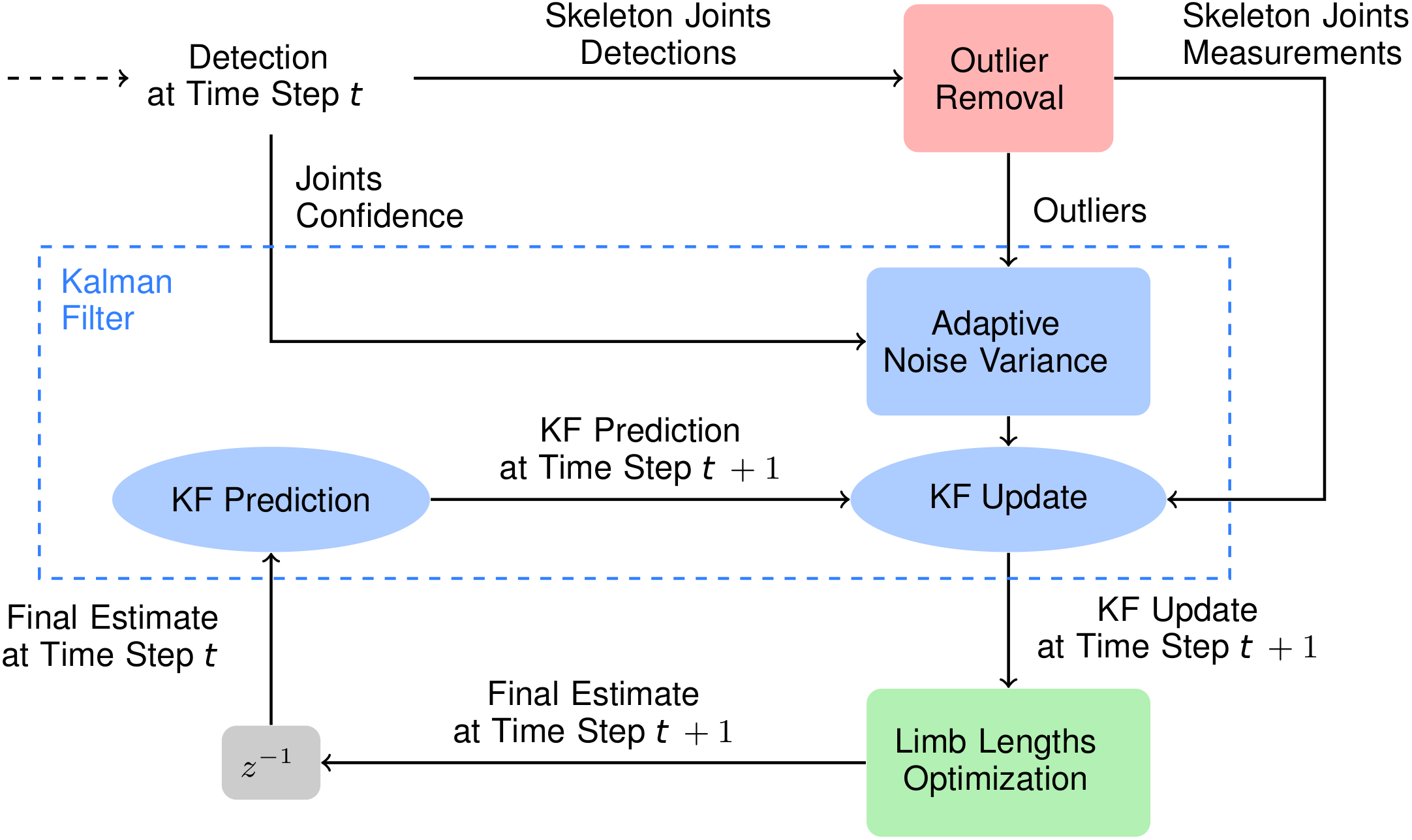
Figure 1: Block scheme representation of the overall tracking procedure.

The body pose estimation system relies on the feed of a camera network composed of $N$ asynchronous RGB-D sensors, thus on sequences of RGB images and depth maps from the different sensors of the network. Neither assumptions on the number of sensor nor on the availability of external aiding tools are made by the system. The only prerequisite is the extrinsic calibration of the camera network. This calibration procedure firstly defines a common global reference frame $\mathcal{G}$ and then computes the matrix $\mathbf{T}\mathcal{{}^{G}_{C}}_{n}$ expressing the relative transformation between the local frame $\mathcal{C}_{n}$ of the $n$-th camera and the global frame $\mathcal{G}$.

The system can be considered as composed by two parts: (i) the single-view detector and (ii) the multi-view fusion algorithm. The first part (i) is the same for each detection node of the network (i.e. the computer in charge of acquiring and processing the data coming only from the camera connected to it). The multi-view fusion algorithm (ii), instead, is executed only by the central processing node which collects and fuses together the estimates provided by the detection nodes.

Although a variety of different solutions to estimate 3D body poses from a single RGB-D sensor exists, in this work we used the one described in [3] which extends the single-view approach described in [14]. Despite our work not being constrained by the specific run-time single-view detection approach, the rationale behind our choice stands in its general applicability since its performances are independent from both the number of people to be tracked and the movements they perform.

III-A Single-view detections identification

The single-view estimates coming from each detection node of the network are fused together by the central processing node. At the generic time $t$, it keeps in memory a set of tracks $\mathfrak{T}^{\mathcal{G}}=\{T^{\mathcal{G}}_{0},\dots,T^{\mathcal{G}}_{l-1}\},\quad l\geq 1$, where the generic $T^{\mathcal{G}}_{j}\in\mathfrak{T}^{\mathcal{G}}$ is defined as the vector of the joint positions of the $j$-th skeleton at time $t$, expressed in the global reference frame. Formally, $T^{\mathcal{G}}_{j}=\{\mathbf{g}_{m}^{\mathcal{G}}=(x_{m}^{\mathcal{G}},y_{m}^{\mathcal{G}},z_{m}^{\mathcal{G}})\,|\,m=1,\dots,M\}$, where $M$ is the number of joints included in the skeleton.

Let us call $\mathfrak{S}^{\mathcal{C}_{n}}$ the generic set of skeletons detected by the $n$-th detection node in its local reference frame $\mathcal{C}_{n}$. Formally, we have $\mathfrak{S}^{\mathcal{C}_{n}}=\{S^{\mathcal{C}_{n}}_{0},\dots,S^{\mathcal{C}_{n}}_{k-1}\}$, where each $S^{\mathcal{C}_{n}}_{i}\in\mathfrak{S}^{\mathcal{C}_{n}}$ is composed of the position of the $M$ joints of the skeleton. Whenever the central processing node receives a new $\mathfrak{S}^{\mathcal{C}_{n}}$ from the $n$-th detection node, it applies the rigid transformation $\mathbf{T}_{\mathcal{C}_{n}}^{\mathcal{G}}$ to express every skeleton in the global reference frame:

$$\mathfrak{S}_{n}^{\mathcal{G}}=\mathbf{T}_{\mathcal{C}_{n}}^{\mathcal{G}}\cdot\mathfrak{S}^{\mathcal{C}_{n}}=\{{S_{n}}^{\mathcal{G}}_{j}=\mathbf{T}_{\mathcal{C}_{n}}^{\mathcal{G}}\cdot{S}^{\mathcal{C}_{n}}_{j},\;\forall{S}^{\mathcal{C}_{n}}_{j}\in\mathfrak{S}^{\mathcal{C}_{n}}\}.$$ (1)

For the ease of reading, in the following the apex $\mathcal{G}$ will be neglected since every quantity has been already expressed in the global reference frame. Furthermore, also the subscript $n$ will be removed from the notation since, if not explicitly stated, we will consider just the generic $n$-th detection node.

The following step performed by the central processing node is data association. The objective is to match each skeleton detected in the current view with its corresponding track, i.e. with its state computed at the previous computation time step. If the algorithm fails to find a matching track for one or more of the detected skeletons within the available ones, it generates a new track for each of them, meaning that persons never seen before walked into the scene.

The problem can be mathematically formulated as an assignment problem. To efficiently solve it, we define the cost of the association of track $T_{i}$ to skeleton $S_{j}$ and we look for the pair skeleton-track which leads to the minimum total cost [27, 28]. We need therefore to compute, at each time $t$, the assignment cost matrix $C_{t}$, where its generic element $c_{i,j,t}$ represents the cost of associating the $j$-th skeleton to the $i$-th track. For each generic $i$-th track among the already available ones, let we call $K_{i}$ the Kalman filter in charge of tracking the position and velocity of its centroid. We first compute $\hat{z}_{i,t|t-1}$, the Kalman filter prediction for the $i$-th track at time $t$ computed without adding any new detection. We then compute, for each skeleton detected at time $t$, $z_{i,j,t}$ as the state of $K_{i}$ at time $t$ under the assumption of associating the $j$-th skeleton to the $i$-th track. The likelihood vector is therefore computed as:

$$\forall T_{i}\in\mathfrak{T},\forall S_{i}\in\mathfrak{S}:\tilde{z}_{i,j,t}=z_{i,j,t}-\hat{z}_{i,t|t-1}\,.$$ (2)

Finally, we compute the cost of the $i,j$-th track-skeleton pair as the Mahalanobis distance between $\tilde{z}_{i,j,t}$ and the covariance matrix $\Sigma_{i}$ of the Kalman filter $K_{i}$. Therefore, each element $c_{i,j,t}$ of the cost matrix $C_{t}$ uses the Mahalanobis distance, where the covariance matrix of the Kalman filter weights the squared norm of the distance vector:

$$c_{i,j,t}=\tilde{z}^{\text{T}}_{i,j,t}\cdot\Sigma_{i}^{-1}\cdot\tilde{z}_{i,j,t}.$$ (3)

At this point, providing the so-constructed matrix $C_{t}$ to the Hungarian algorithm [27], also known as Munkres algorithm [28], we solve the assignment problem finding the optimal pairing between tracks and detections. However, since that algorithm does not directly implement a constraint on the maximum distance between tracks and detections, a threshold $\epsilon$ is introduced to reduce the probability of wrong associations. Given a skeleton, if its distance from all the tracks is higher than $\epsilon$ , than it does not match any of them, meaning that it corresponds to a new person on the scene and, therefore, a new track for him needs to be created.

III-B Multi-view skeletal fusion

Once the single-view detections identification is completed, the tracks are given as input to the proposed processing pipeline (Fig. 1). The whole algorithm is based on the association of each track with a $6M$-dimensional Kalman filter, where $M=15$ is the number of joints. From this point on, for ease of reading, just one track is considered since all the tracks are treated as separate entities and processed following exactly the same pipeline.

The state $\mathbf{x}_{t}$ of the Kalman filter at time $t$ is constructed by juxtaposition, for each $m$-th joint, of its 3D position $\mathbf{q}_{m}=[x_{m},y_{m},z_{m}]$ and velocity $\mathbf{\dot{q}}_{m}=[\dot{x}_{m},\dot{y}_{m},\dot{z}_{m}]$. Formally:

$$\mathbf{x}_{t}=\{\left[\mathbf{q}_{m}\rvert\mathbf{\dot{q}}_{m}\right]_{t}^{T}\,|\,m=1,\dots,M\}.$$ (4)

The prediction phase of the Kalman filter is driven by the following constant velocity evolution model:

$$\mathbf{x}_{t+1}=\mathbf{F}\mathbf{x}_{t}+\mathbf{G}\mathbf{n}\,,$$ (5)

where $\mathbf{F}\in\mathbb{R}^{6M\times 6M}$ is the transition matrix that implements the constant velocity prediction for each component. In other words, at time step $t+1$, the velocity part of the state is predicted to be equal to the previous one ($\mathbf{\dot{q}}_{m,t+1}=\mathbf{\dot{q}}_{m,t}$), while the position part evolves as $\mathbf{q}_{m,t+1}=\mathbf{q}_{m,t}+\Delta t\cdot\mathbf{\dot{q}}_{m,t}$, where $\Delta t$ is the sampling period. We use $\Delta t=33\,\text{ms}$, because $30\,\text{Hz}$ is the maximum frame-rate of our sensor. In case of heavy occlusions, a normal situation in multi-persons scenarios, it is likely that the time interval between two consecutive detections of the same full skeleton can be approximated to an integer multiple of $\Delta t$. Therefore, letting the time interval between two consecutive detections be $n\cdot\Delta t$, the prediction step is computed $n$ times. $\mathbf{G}\in\mathbb{R}^{6M\times 3M}$ is the noise coupling matrix that describes how the elements of the Gaussian white noise vector $\mathbf{n}\sim\mathcal{N}(\mathbf{0},\sigma_{q}^{2}\cdot\mathbf{1}^{3M\times 1})$ affect the system.

The observations at time $t+1$ are represented by the 3D joint positions of the identified skeleton in the global reference frame. Therefore, the measurement model is:

$$\mathbf{y}_{t+1}=\mathbf{H}\mathbf{x}_{t+1}+\mathbf{w},$$ (6)

where

$$\mathbf{H}=\left[\begin{array}[]{ccc|ccc}1&&&0&&\\ &\ddots&&&\ddots&\\ &&1&&&0\end{array}\right].$$ (7)

The meaning of $\mathbf{H}\in\mathbb{R}^{3M\times 6M}$ is straightforward, and the measurement noise vector is defined as Gaussian white noise $\mathbf{w}\sim\mathcal{N}(\mathbf{0},\sigma_{r}^{2}\cdot\mathbf{1}^{3M\times 1})$.

Once defined the structure of the Kalman filters, we need to find the values of the noise variances. In the presented work, we estimated the measurement noise variance offline from a prerecorded static sequence available in our dataset. We therefore computed the value of $\sigma_{r}^{2}$ by averaging, through all the joints, the standard deviation of the joint positions in all the detections of the sequence. As the careful reader may notice, this is an approximation, given that this value might be variable in different spots of the scene due to a non-perfectly uniform calibration of the camera network.

The process noise variance, on the other hand, cannot be computed using the same offline procedure since it is dependent from the movements performed by the people in the scene. Therefore, a manual tuning of the process noise variance has been performed.

III-C Joint confidence feedback

The basic concept of Bayesian filtering is the inclusion of a-priori information in the estimation process. Starting from this consideration, we preprocess the detections coming from each single-view detection node to gain insights to be included in the system state. The single-view detector returns, for each $m$-th joint of each detection, its 3D position and the associated confidence level $c_{m}\in[0,1]$. In order to include this information in our estimation procedure, we implement an adaptive scheme that determines, at time step $t$, the measurement noise variance of $\mathbf{q}_{m}$, i.e. $\sigma^{2}_{rc,m_{x}},\sigma^{2}_{rc,m_{y}},\sigma^{2}_{rc,m_{z}}$ in relation to $c_{m}$:

$$\sigma^{2}_{rc,m,t}=\sigma^{2}_{rc,m_{x},t}=\sigma^{2}_{rc,m_{y},t}=\sigma^{2}_{rc,m_{z},t}=\frac{\sigma^{2}_{r}}{c_{m}}.$$ (8)

In order to reduce the tracking errors coming from highly uncertain detections, we use a threshold of $th=0.5$ to filter them out. Therefore, if $c_{m}<th$, the joint detection is rejected and substituted with the Kalman filter prediction at time $t$ ($\hat{y}_{t|t-1}$).

III-D Outlier filtering

One of the most important advantages of camera networks is the possibility to overcome occlusions and inconsistencies typical of the single-view detections which generally lead to huge spikes in joint position estimates. To filter out the so-called outliers, we introduce an adaptive scheme that updates the measurement reliability, based on the recent history of the tracked joint, to prevent too rapid changes in its position. We consider the Euclidean distance between consecutive positions of the same joint. Once a threshold is determined, the new measurement is considered unreliable if the distance value from the previous state is above the threshold. In our algorithm we use, for each $m$-th joint, a slow time-varying threshold $th_{m}$ that takes into account the information from the joint history. The idea is to consider the consecutive distances between the previous $N$ samples of the joint position $d_{m,t-i}$, where $i=1,\dots,N$. The threshold at time $t$ is therefore computed as:

$$th_{m,t}=w\cdot\max\{d_{m,t-i},\,i=1,\dots,N\},$$ (9)

where $w\geq 1\in\mathbb{R}$. In this way, the joint-specific threshold is potentially capable of slowly adapting to the changes in joint speed.

If the new detection distance for the $m$-th joint $d_{m,t}$ is larger than the just computed threshold $th_{m,t}$, the detection is not directly rejected, but the corresponding measurement noise variance, after the joint confidence adaptation, is updated as follow:

$$\text{if}\,\;d_{m,t}>th_{m,t}\;\;\Rightarrow\;\;\sigma^{2}_{ro,m,t}=\frac{\sigma^{2}_{rc,m,t}}{th_{m,t}/d_{m,t}}.$$ (10)

A possible limitation of this approach might be that correct detections describing a very fast motion of a joint could be detected as outliers. To overcome this limitation we introduced the parameter $o_{max}$, which represents the maximum number of consecutive outliers a track can accept. In this way, even if $o_{max}$ consecutive measurements are detected as outliers, the next one is considered reliable and used to update the track. In practice we chose $o_{max}=2$, based on the idea that, being in a network, if one detection node is experiencing an occlusion leading to an outlier, hopefully the next detection will come from another detection node not experiencing the same occlusion.

III-E Skeleton consistency

A typical problem in skeletal tracking from images is the segment length variability. Indeed, the distance between two adjacent joints might vary depending on their relative position estimated from images taken from different viewing angles. To overcome this limitation, we introduce an algorithm which aims at keeping the segment lengths constant during the whole tracking process. While the Kalman filter presented in the previous sections focuses on ensuring temporal coherence, this section aims at discussing the algorithm introduced to guarantee the physical consistency of the tracked skeletons.

At each time step $t$, the physical consistency algorithm takes as input the system state $\mathbf{x}_{t}$, and the hierarchical model of the human body (Fig. 2).

Figure 2: Hierarchical model of the human body. The nodes represent the joints while the connecting lines the body links.

Head and chest joints have been excluded from the optimization for two reasons. On the one hand, we obtained more stable results computing the chest as the central point between shoulders and hips. On the other hand, the head has been removed since out of interest for this preliminary assessment. However, the developed implementation of the algorithm already supports the inclusion of those two joints. At the time $t$ (dependency omitted for the ease of reading), for each $i$-th link of the filtered skeleton track ($i\in 1\dots L$, with $L$ number of links of the skeleton model), we compute the energy of its length error:

$$E_{i}=(\|\mathbf{q}_{c,i}-\mathbf{q}_{p,i}\|-\hat{l}_{i})^{2}$$ (11)

where $\mathbf{q}_{c,i}$ and $\mathbf{q}_{p,i}$ are the 3D coordinates of, respectively, the child and parent joints of the $i$-th link. While $\mathbf{q}_{c,i}$ is the output of the current link length optimization, $\mathbf{q}_{p,i}$ is the output of the length optimization of the previous link of the hierarchical model. Initial values for $\mathbf{q}_{c,i}$ are set equal to the estimates of the Kalman filter $\mathbf{\hat{q}}_{c,i}$.

We initialize $\hat{l}_{i}$ for each link using the average of the limb lengths measured in the first few frames in which the entire skeleton is completely tracked. Then, after the optimization, the estimated lengths are updated using the just computed joint coordinates to slowly compensate possible inaccurate link lengths initializations. In order to avoid jitters in the final estimates due to local minima computed by the minimization of the energy defined as in Eq. 11, we add a second term which accounts for link orientation errors. Therefore, we re-defin $E_{i}$ as:

$$E_{i}=(\|\mathbf{q}_{c,i}-\mathbf{q}_{p,i}\|-\hat{l}_{i})^{2}+(\|\text{\boldmath$\theta$}_{i}-\text{\boldmath$\theta$}_{kf,i}\|)^{2}$$ (12)

where:

$$\text{\boldmath$\theta$}_{i}=\frac{\mathbf{q}_{c,i}-\mathbf{q}_{p,i}}{\|\mathbf{q}_{c,i}-\mathbf{q}_{p,i}\|}\\ ,\quad\text{\boldmath$\theta$}_{kf,i}=\frac{\mathbf{q}_{kf,c,i}-\mathbf{q}_{p,i}}{\|\mathbf{q}_{fk,c,i}-\mathbf{q}_{p,i}\|}\\$$ (13)

The unitary vectors $\text{\boldmath$\theta$}_{i}$ and $\text{\boldmath$\theta$}_{kf,i}$ describe, respectively, the orientation of the $i$-th link during the optimization process and the original link orientation estimated by the Kalman filter. To solve this energy minimization problem we use the Levenberg-Marquardt algorithm implemented in the Ceres Solver library.

IV Experiments and Results

In order to highlight the efficacy of the proposed approach, given the lack of publicly available RGB-D camera-network datasets, a new one has been recorded. We are currently working to make our dataset public. To record the dataset, we asked different subjects to perform free movements in the scene. We recorded data from a camera network composed by 4 Kinect v2 cameras and, at the same time, the output of a commercial motion capture system (BTS SMART-DX, BTS Bioengineering Corp., USA). Each subject was instrumented with a set of passive reflective markers attached to the skin following the BTS standard marker placing protocol.

The 4 Kinects were placed at the four corners of the considered motion area, while the 12 SMART-DX cameras were equally spaced along the perimeter. Both the Kinects and the SMART-DX cameras were placed at a height of approximately 2.5 m. Noteworthy, the two systems acquire data at different frequencies: 30 fps for the Kinect sensor network, and 50 fps for the SMART-DX cameras. A time synchronization mechanism for relating each Kinect data point with the corresponding reference was therefore set up.

After completing the calibration procedures of both the systems, we recorded three static sequences (15 seconds each) and six dynamic sequences (approx. 60 seconds each). Each dynamic sequence is characterized by different motion characteristics (i.e. fast or slow movements) performed by a different number of subjects (one or two). While the static sequences have been used for tuning systems parameters, the dynamic ones have been used to assess the accuracy of the proposed approach against the gold-standard results provided by the BTS system.

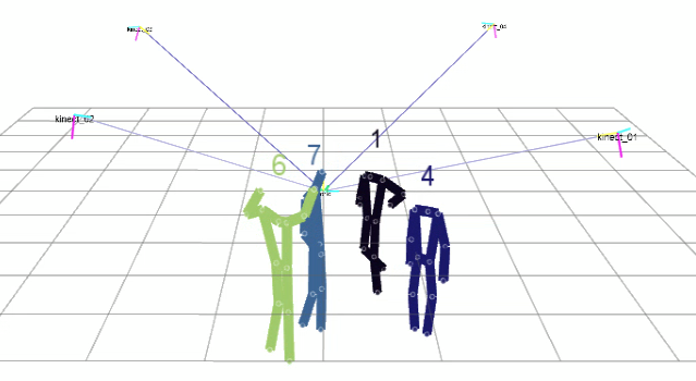
Figure 3: Typical output of the proposed system. Kinematic tracking of four persons at the same time.

Fig. 3 shows an example of the virtual scene where the four identified skeletons (the subject ID is presented as the number over the skeleton) replicating the real subject movements.

The evaluation was conducted using as overall metrics the average and standard deviation of the joints displacement tracking errors among all the joints. In particular, after the interpolation step, for each $m$-th joint, we compare the estimated 3D position and the corresponding ground truth, respectively named $\mathbf{q}_{\text{est,m}}$ and $\mathbf{q}_{\text{gt,m}}$. Then, given the sequences of $N$ time samples $\{\mathbf{Q}_{\text{est},1},\dots,\mathbf{Q}_{\text{est},N}\}$ and $\{\mathbf{Q}_{\text{gt},1},\dots,\mathbf{Q}_{\text{gt},N}\}$, where $\mathbf{Q}_{\text{est},i}=\sum_{m=1}^{M}\mathbf{q}_{\text{est,m,i}}$ and $\mathbf{Q}_{\text{gt},i}=\sum_{m=1}^{M}\mathbf{q}_{\text{gt,m,i}}$, the two evaluation metrics are defined as:

$$e_{\text{avg}} =\frac{\sum_{i=1}^{N}\|\mathbf{Q}_{\text{est},i}-\mathbf{Q}_{\text{gt},i}\|}{N},$$ (14)

$$e_{\text{sd}} =\sqrt{\frac{\sum_{i=1}^{N}(\|\mathbf{Q}_{\text{est},i}-\mathbf{Q}_{\text{gt},i}\|-e_{\text{avg}})^{2}}{N}}.$$

For all the six sequences, we computed the same performance metrics (average joint displacement error and standard deviation) on the estimates provided by other state-of-the-art approaches using as input exactly the same data from all the four available Kinects. The other comparison methods have been: (i) OpenPose [14] enriched with the data association and depth inference algorithms, (ii) moving average filtering (MAF), a common baseline approach already described in other similar state-of-the-art works such as [3, 19], and (iii) the standard version of OpenPTrack [3]. The obtained results are reported in Table I.

TABLE I: Joint displacement tracking errors of the four systems considered for comparison. The proposed approach in bold. Results reported in $cm$ as mean $\pm$ sd.

Sequence and	OpenPose [14]	MAF	OpenPTrack [3]	Proposed
Subject				Solution
Seq. 1	$8.29\pm 7.39$	$12.56\pm 7.17$	$11.85\pm 6.4$	$\mathbf{5.55\pm 2.68}$
Seq. 2	$9.47\pm 8.43$	$17.16\pm 10.23$	$14.84\pm 8.67$	$\mathbf{7.41\pm 4.74}$
Seq. 3	$8.79\pm 7.42$	$14.48\pm 7.35$	$14.17\pm 6.2$	$\mathbf{6.74\pm 3.76}$
Seq. 4	$11.33\pm 8.81$	$20.68\pm 9.44$	$18.56\pm 8.24$	$\mathbf{9.53\pm 4.46}$
Seq. 5, Sbj. 1	$8.81\pm 8.74$	$14.98\pm 7.98$	$13.17\pm 6.63$	$\mathbf{6.45\pm 3.52}$
Seq. 5, Sbj. 2	$9.01\pm 9.11$	$20.73\pm 10.85$	$17.31\pm 8.86$	$\mathbf{7.43\pm 5.53}$
Seq. 6, Sbj. 1	$9.94\pm 9.25$	$20.93\pm 10.9$	$17.62\pm 8.91$	$\mathbf{8.55\pm 5.1}$
Seq. 6, Sbj. 2	$9.74\pm 8.71$	$19.75\pm 9.82$	$16.11\pm 8.28$	$\mathbf{8.05\pm 4.31}$

The results clearly show how the proposed multi-subject kinematics tracking approach outperforms, in terms of joint displacement errors, the other considered state-of-the-art systems. Moreover, it is worth noticing that in the fifth and sixth sequences the two subjects on the scene were tracked at the same time, demonstrating the absence of accuracy drops in multi-user applications of our system.

As an additional evaluation metric for the proposed system, we investigated the consistence of the estimates quality when the network is composed by a lower number of cameras. To do that we selected, for every available sequence, data coming just from two, three, or four detection nodes. Fig. 4 shows how the estimation quality increases with the number of cameras installed in the network.

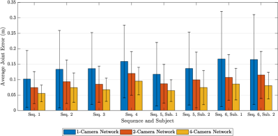
Figure 4: Tracking performance comparison, in terms of mean joint error and standard deviation averaged on all joints, using networks of different sizes. The thin bars in the graph indicate an interval of one standard deviation around the error mean.

Furthermore, it is important to observe that such performances were obtained while producing the body pose estimates in real-time (tested on an Intel Core i7-4770 CPU and Nvidia GeForce GTX 1060 GPU powered desktop). In a typical iteration, the average computational time (approx. $13.4\,ms$) is distributed among the different major processes as follow:

• $\sim 40\,\mu s$ for the adaptive scheme with the outlier detection, the iterative computation of the outlier thresholds, and the iterative estimate of the limb lengths;

• $\sim 3$ – $5\,ms$ for the limb lengths optimization;

• $\sim 5$ – $7\,ms$ for the update step of the Kalman filter;

• $\sim 1\,ms$ for other computational activities.

TABLE II: Theoretical and real computational times of our systems depending on the number of subjects to track.

Tracked	Worst case comp. time	Worst case fps	Experimental fps
persons	$[ms]$	(theoretical)
1	$\sim 13.4$	$\sim 74.6$	$33.9$
2	$\sim 26.8$	$\sim 37.3$	$32.1$
3	$\sim 40.2$	$\sim 24.9$	–
4	$\sim 53.6$	$\sim 18.7$	$18.7$
5	$\sim 67.0$	$\sim 14.9$	–
6	$\sim 80.4$	$\sim 12.4$	–

Table II reports how the theoretical output frame rate scales with the number of subjects to be tracked by our system. In case of up to two subjects the actual tracking output frame rate is however lower than the theoretical one due to the input data frequency constraint; indeed, the Kinect cameras are capable of providing data at maximum at $30\,fps$. In case of three or more persons, instead, the most restrictive limit becomes the computational time, with an actual tracking frame rate which scales proportionally to the number of subjects to track. Setting a limit for considering an application as real-time to be equal to $15\,fps$, it is shown that for cases of up to 5 persons in the scene our approach satisfies this constraint.

V Conclusions

In this work we proposed, discussed, and evaluated an innovative markerless approach to accurately estimate and the track human motion in real-time through a calibrated network of RGB-D cameras. The proposed methodology demonstrated to be reliable and accurate in tracking multiple persons at the same time, without requiring the subjects to perform initial calibration activities or to wear any marker. The developed system requires neither a specific number of cameras in the network, nor all the cameras to be of the same manufacturer; moreover, it does not require the cameras to be synchronized. These three valuable features enable users to build their own heterogeneous network following their specific needs and possibilities.

Starting from the noisy single-frame single-view detections, our algorithm ensures temporal and physical consistency during the whole tracking period. As demonstrated by the obtained results, it reduces the joint displacement tracking error, with respect to the current state-of-the-art approaches used as reference for the comparison. Moreover, the proposed approach is not only reliable and effective, but also efficient, enabling to track in real-time up to 5 subjects at the same time. This is indeed a crucial capability, since it is a major requirement for the large majority of the applications in the human-robot interaction field.

References

- [1] M. Carraro, M. Munaro, and E. Menegatti, “A powerful and cost-efficient human perception system for camera networks and mobile robotics,” in International Conference on Intelligent Autonomous Systems. Springer, 2016, pp. 485–497.
- [2] S. Särkkä, V. Tolvanen, J. Kannala, and E. Rahtu, “Adaptive kalman filtering and smoothing for gravitation tracking in mobile systems,” in Indoor Positioning and Indoor Navigation (IPIN), 2015 International Conference on. IEEE, 2015, pp. 1–7.
- [3] M. Carraro, M. Munaro, J. Burke, and E. Menegatti, “Real-time marker-less multi-person 3d pose estimation in rgb-depth camera networks,” arXiv preprint arXiv:1710.06235, 2017.
- [4] N. Sarafianos, B. Boteanu, B. Ionescu, and I. A. Kakadiaris, “3d human pose estimation: A review of the literature and analysis of covariates,” Computer Vision and Image Understanding, vol. 152, pp. 1–20, 2016.
- [5] F. Han, X. Yang, C. Reardon, Y. Zhang, and H. Zhang, “Simultaneous feature and body-part learning for real-time robot awareness of human behaviors,” in IEEE International Conference on Robotics and Automation (ICRA), 2017, pp. 2621–2628.
- [6] M. Zanfir, M. Leordeanu, and C. Sminchisescu, “The moving pose: An efficient 3d kinematics descriptor for low-latency action recognition and detection,” in Proceedings of the IEEE International Conference on Computer Vision, 2013, pp. 2752–2759.
- [7] S. Ghidoni and M. Munaro, “A multi-viewpoint feature-based re-identification system driven by skeleton keypoints,” Robot. Auton. Syst., vol. 90, no. C, pp. 45–54, Apr. 2017. [Online]. Available: https://doi.org/10.1016/j.robot.2016.10.006
- [8] A. Jaimes and N. Sebe, “Multimodal human–computer interaction: A survey,” Computer vision and image understanding, vol. 108, no. 1, pp. 116–134, 2007.
- [9] D. McColl, Z. Zhang, and G. Nejat, “Human body pose interpretation and classification for social human-robot interaction,” International Journal of Social Robotics, vol. 3, no. 3, pp. 313–332, 2011.
- [10] A. Gupta, S. Satkin, A. A. Efros, and M. Hebert, “From 3d scene geometry to human workspace,” in Computer Vision and Pattern Recognition (CVPR), 2011 IEEE Conference on. IEEE, 2011, pp. 1961–1968.
- [11] C. Morato, K. N. Kaipa, B. Zhao, and S. K. Gupta, “Toward safe human robot collaboration by using multiple kinects based real-time human tracking,” Journal of Computing and Information Science in Engineering, vol. 14, no. 1, p. 011006, 2014.
- [12] C. Chen and J.-M. Odobez, “We are not contortionists: Coupled adaptive learning for head and body orientation estimation in surveillance video,” in Computer Vision and Pattern Recognition (CVPR), 2012 IEEE Conference on. IEEE, 2012, pp. 1544–1551.
- [13] C. Chen, A. Heili, and J.-M. Odobez, “Combined estimation of location and body pose in surveillance video,” in Advanced Video and Signal-Based Surveillance (AVSS), 2011 8th IEEE International Conference on. IEEE, 2011, pp. 5–10.
- [14] Z. Cao, T. Simon, S.-E. Wei, and Y. Sheikh, “Realtime multi-person 2d pose estimation using part affinity fields,” 2017 IEEE Conference on Computer Vision and Pattern Recognition (CVPR), pp. 1302–1310, 2017.
- [15] D. Mehta, S. Sridhar, O. Sotnychenko, H. Rhodin, M. Shafiei, H.-P. Seidel, W. Xu, D. Casas, and C. Theobalt, “Vnect: Real-time 3d human pose estimation with a single rgb camera,” ACM Transactions on Graphics (TOG), vol. 36, no. 4, p. 44, 2017.
- [16] Z. Zivkovic, “Wireless smart camera network for real-time human 3d pose reconstruction,” Computer Vision and Image Understanding, vol. 114, no. 11, pp. 1215–1222, 2010.
- [17] M. Carraro, M. Munaro, and E. Menegatti, “Cost-efficient rgb-d smart camera for people detection and tracking,” Journal of Electronic Imaging, vol. 25, pp. 041 007–041 007, 04 2016.
- [18] K. Buys, C. Cagniart, A. Baksheev, T. De Laet, J. De Schutter, and C. Pantofaru, “An adaptable system for rgb-d based human body detection and pose estimation,” Journal of visual communication and image representation, vol. 25, no. 1, pp. 39–52, 2014.
- [19] M. Carraro, M. Munaro, A. Roitberg, and E. Menegatti, “Improved skeleton estimation by means of depth data fusion from multiple depth cameras,” in International Conference on Intelligent Autonomous Systems. Springer, 2016, pp. 1155–1167.
- [20] S. Moon, Y. Park, D. W. Ko, and I. H. Suh, “Multiple kinect sensor fusion for human skeleton tracking using kalman filtering,” International Journal of Advanced Robotic Systems, vol. 13, no. 2, p. 65, 2016.
- [21] M. Caon, Y. Yue, J. Tscherrig, E. Mugellini, and O. A. Khaled, “Context-aware 3d gesture interaction based on multiple kinects,” in Proceedings of the first international conference on ambient computing, applications, services and technologies, AMBIENT. Citeseer, 2011, pp. 7–12.
- [22] S. Kaenchan, P. Mongkolnam, B. Watanapa, and S. Sathienpong, “Automatic multiple kinect cameras setting for simple walking posture analysis,” in Computer Science and Engineering Conference (ICSEC), 2013 International. IEEE, 2013, pp. 245–249.
- [23] G. Liu, G. Tian, J. Li, X. Zhu, and Z. Wang, “Human action recognition using a distributed rgb-depth camera network,” IEEE Sensors Journal, vol. 18, no. 18, pp. 7570–7576, 2018.
- [24] A. T. Kamal, J. H. Bappy, J. A. Farrell, and A. K. Roy-Chowdhury, “Distributed multi-target tracking and data association in vision networks,” IEEE transactions on pattern analysis and machine intelligence, vol. 38, no. 7, pp. 1397–1410, 2016.
- [25] S. Ershadi-Nasab, E. Noury, S. Kasaei, and E. Sanaei, “Multiple human 3d pose estimation from multiview images,” Multimedia Tools and Applications, vol. 77, no. 12, pp. 15 573–15 601, 2018.
- [26] M. Munaro, F. Basso, and E. Menegatti, “Openptrack: Open source multi-camera calibration and people tracking for rgb-d camera networks,” Robotics and Autonomous Systems, vol. 75, pp. 525–538, 2016.
- [27] H. W. Kuhn, “The hungarian method for the assignment problem,” Naval Research Logistics (NRL), vol. 2, no. 1-2, pp. 83–97, 1955.
- [28] J. Munkres, “Algorithms for the assignment and transportation problems,” Journal of the society for industrial and applied mathematics, vol. 5, no. 1, pp. 32–38, 1957.