Removing the Wigner bound in non-perturbative effective field theory

Abstract

The Wigner bound, setting an upper limit on the scattering effective range, is examined at different orders of contact effective field theory. Using cutoff regulator we show that the bound loosens when higher orders of the theory are considered. For a sharp and a Gaussian regulators, we conjecture an analytic formula for the dependence of the Wigner bound on the theory’s order. It follows that the bound vanishes in the limit of infinite order.

Using a concrete numerical example we demonstrate that the above surmise still holds after renormalization at finite cutoff. Studying the 3-body system with this example, we have found that limiting the permissible range of cutoffs by the Wigner bound, we avoid the Thomas collapse, and don’t need to promote the 3-body force to leading order.

I Introduction

In the last two decades contact effective field theory (EFT) has been successfully applied for studying low energy systems where the characteristic particle wave length is much larger than the interaction range. Such systems can be found, for example, in ultra cold atomic gases, clusters of He atoms, and atomic nuclei, see e.g. Higa2008 ; Braaten2006 ; Hammer2017 ; Hammer2019 . In such circumstances, it can be argued that the details of the short-range part of the interaction become irrelevant and a contact interaction, i.e. a delta function and its derivatives, can be used to parameterize it Lepage1997 ; Bedaque2002 ; Beane2000 . This parameterization can be understood to result from integrating out the high energy degrees of freedom of the underlying theory and then expanding the resulting Lagrangian in terms of contact interactions.

In a complete EFT, the Lagrangian should include all possible terms compatible with the symmetries of the underlying theory. To make such theory of any use, only finite number of terms should be retained when aiming to calculate some observable to a desired accuracy. Therefore an appropriate ordering of the Lagrangian terms is a key ingredient for a successful EFT. A natural order for contact EFT is arranging the interaction terms according to their mass dimension Kaplan2005 ; Hammer2019 ; Epelbaum2017 . A non-relativistic particle field $\Psi$ counts as $3/2$ and a derivative counts as $1$. This ordering is known as the “naïve” power counting. It works very well for the 2-body sector if the scattering length $a_{s}$ is of the order of the interaction range, but fails for very large scattering lengths (see e.g. PavonValderama2017 for a nice derivation), and for the $3,4,\ldots$-body, interaction terms BHvK99 ; Bazak2018a .

In the scheme proposed by Weinberg Weinberg1990 , the contact interactions are to be iterated in the Lippmann-Schwinger equation to yield the $T$-matrix. Analyzing the ability of such a scheme to reproduce the low energy $s$-wave effective range expansion, the scattering length and effective range $r_{\text{eff}}$, Phillips et al. Phillips1997 ; Phillips1998 have argued, using cutoff regulation, that the resulting effective range is necessarily negative in the limit of infinite cutoff, $\Lambda\to\infty$. Furthermore, analyzing specifically a contact EFT at next-to-leading-order (NLO) with a 2-body potential consisting of a delta function plus its derivative-squared, they have shown that in the $\Lambda\to\infty$ limit $r_{\text{eff}}\leq 0$ regardless of the Lagrangian parameterization, i.e. the value of the low energy constants (LECs).

The deep fundamental reason behind this observation can be traced back to the causality principle. For a scattering process, causality implies that the scattered wave cannot leave the target before the incident wave has reached it. Applying this argument to 2-body scattering with an energy independent potential of range $R$, Wigner has shown Wigner1955 , followed by others Hammer2010 ; Phillips1997 , that the effective range has an upper bound,

$$r_{\text{eff}}\leq 2R\left(1-\frac{R}{a_{s}}+\frac{R^{2}}{3a_{s}^{2}}\right)\;.$$ (1)

The range $R$ of the interaction is proportional to $1/\Lambda$. Hence, the Wigner bound becomes more restrictive with increasing $\Lambda$. In the limit of $\Lambda\to\infty$ ($R\to 0$), the effective range is bounded from above by zero Phillips1998 .

This bound has a profound effect on contact EFT. The theory cannot be renormalized while working non-perturbatively Beane1998 . More precisely, the cutoff cannot be eliminated without turning $r_{\text{eff}}$ to be negative, if any order but the leading order is treated non-perturbatively vanKolck1999 . Consequently, two options remain, either working non-perturbatively giving up renormalization group invariance, see e.g. Bansel2018 ; Lensky2016 , or working perturbatively for any EFT order beyond leading order, see e.g. Hammer2017 . The latter option is much harder numerically for the many-body problem, since it requires resolving the full leading order Green’s function.

Here we would like to take a second look at non-perturbative contact EFT, and check if it is forever doomed to be cutoff dependent or maybe renormalization group invariance can be restored if we include enough orders in our calculation. Put differently - what will happen if we first take infinite EFT orders and only then push the cutoff to infinity? As a motivation consider the EFT as a sum of delta functions and their derivatives Lepage1997 , generated from a Gaussian with a width of $\frac{1}{\Lambda}$. In the limit $\Lambda\to\infty$ the delta function is recovered. For higher EFT orders the interaction range is associated with terms of the form $x^{n}\exp(-x^{2}/2)$, i.e. higher order terms broaden the interaction range. For a specific order the resulting range is finite and by taking $\Lambda\to\infty$ the range vanishes. But this may not be the case for infinite EFT order where there are infinite number of terms which broadens the interaction range.

To study this point we consider here a contact EFT of scalar bosonic fields. First we show explicitly using partial renormalization that up to order N⁹LO, given a scattering length, the Wigner bound loosens as more EFT orders are taken into account. Then we demonstrate, for a concrete example at N²LO, that our finding holds when the LECs are renormalized to reproduce the effective range expansion to order $p^{4}$. From this analysis we conjecture that for an arbitrary value of $\Lambda$, any finite effective range $r_{\text{eff}}$ can be described by the theory if the EFT order is large enough. In the process, we find that multiple renormalization choices arise as more orders are taken into account. A method to pick the physical one is then suggested.

II Effective range in increasing EFT orders

In order to understand the evolution of the Wigner bound with increasing EFT orders, we study a low energy EFT for a scalar bosonic field $\Psi$ of mass $m$. This theory is closely related to the nuclear pionless effective field theory ($\not{\pi}$EFT ), that as fundamental degrees of freedom includes only nucleons, with no mesons. Starting from the EFT Lagrangian ${\cal L}$, and deducing the 2-body interaction, the low energy scattering parameters are obtained by solving the $s$-wave Lippmann-Schwinger equation. Expanding the resulting $T$-matrix in the usual low-momentum form

$$\frac{1}{T}=-\frac{m}{4\pi}\left(-\frac{1}{a_{s}}+\frac{1}{2}r_{\text{eff}}~{}p^{2}+\sum_{n\geq 2}S_{n}p^{2n}-ip\right),$$ (2)

the scattering length $a_{s}$ is then identified as the leading momentum independent term, the effective range $r_{\text{eff}}$ as the energy $p^{2}$ coefficient, and the shape parameters $S_{n}$ through the $p^{2n}$ terms.

Considering only $s$-wave interactions, and ignoring 3-body and higher multi-particle interaction terms, the EFT Lagrangian can be written as

$${\cal L}={\cal L}_{0}+{\cal L}_{1}+{\cal L}_{2}+\ldots$$ (3)

where ${\cal L}_{0}$, the LO Lagrangian, includes the free Lagrangian and a contact interaction term

$${\cal L}_{0}=\Psi^{\dagger}\left(i\partial_{t}+\frac{1}{2m}\nabla^{2}\right)\Psi-\frac{1}{4}C_{00}\left(\Psi^{\dagger}\Psi\right)^{2}\;,$$ (4)

${\cal L}_{1}$ includes the subleading NLO interaction term

$${\cal L}_{1}=-\frac{1}{8}{C_{20}}\left[\left(\Psi^{\dagger}\Psi\right)\left(\Psi^{\dagger}\nabla^{2}\Psi\right)+h.c.\right]\;,$$ (5)

and ${\cal L}_{2}$ the N²LO interaction term

$${\cal L}_{2}= -\frac{1}{8}{C_{40}}\left[\left(\Psi^{\dagger}\Psi\right)\left(\Psi\nabla^{4}\Psi^{\dagger}\right)+h.c.\right]$$ (6)

$$-\frac{1}{4}C_{22}\left(\Psi^{\dagger}\nabla^{2}\Psi\right)\left(\Psi^{\dagger}\nabla^{2}\Psi\right)\;.$$ (7)

In a similar fashion, ${\cal L}_{n}$ includes all possible 4-field operators with $n$ insertions of $\nabla^{2}$. The Lagrangian parameters $C_{pq}$, known as the low energy coefficients (LECs), are fixed through the renormalization condition to reporoduce the scattering parameters $a_{s},r_{\text{eff}},S_{n}$, etc. For brevity, we also write $C_{00}$ as $C_{0}$, $C_{20}$ as $C_{2}$, and so on.

In momentum space, the corresponding potential can be written as

$$V_{\text{N}^{n}\text{LO}}= C_{0}+C_{2}\left(p^{2}+p^{\prime 2}\right)$$ (8)

$$\hskip 10.00002pt+C_{4}\left(p^{4}+p^{\prime 4}\right)+C_{22}p^{2}p^{\prime 2}+\cdots\;,$$ (9)

where ${\boldsymbol{p}}$ is the incoming relative momentum and ${\boldsymbol{p}}^{\prime}$ the outgoing momentum. To avoid the UV divergences embedded in the contact terms we regularize the interaction $V\to F({\boldsymbol{p}}^{\prime})VF({\boldsymbol{p}})$ using either a Gaussian regulator $F(p)=e^{-\frac{p^{2}}{\Lambda^{2}}}$ or a sharp cutoff $F(p)=\Theta(\Lambda-p)$, where $\Theta(\Lambda-p)$ is the Heaviside step function.

The $T$-matrix is obtained by iterating the potential through the Lippmann-Schwinger equation

$$T=V+VGT\;.$$ (10)

Following the footsteps of Phillips, Beane and Cohen Phillips1998 , we note that for a separable potential such as the EFT interaction (8), which can be written as

$$V(p,p^{\prime})=F(p)\sum_{i,j=0}^{n}p^{2i}\lambda_{ij}p^{\prime 2j}F(p^{\prime})\;,$$ (11)

the $T$-matrix assumes the form

$$T(E)=F(p)\sum_{i,j=0}^{n}p^{2i}\tau_{ij}(E)p^{\prime 2j}F(p^{\prime})\;,$$ (12)

and the Lippmann-Schwinger equation is reduced into a simple matrix equation

$$\tau(E)=\lambda+\lambda{\cal I}(E)\tau(E)$$ (13)

where the matrix elements of ${\cal I}$ are given by

$${\cal I}_{ij}\equiv\int\frac{d^{3}q}{(2\pi)^{3}}\frac{F^{2}(q)q^{2(i+j)}}{E+i\varepsilon-\frac{q^{2}}{2\mu}}\;$$ (14)

and $\mu=m/2$ is the reduced mass. Equation (13) can be formally solved to yield

$$\tau(E)=\frac{1}{1-\lambda{\cal I}(E)}\lambda\;.$$ (15)

The matrix elements $\lambda_{ij}$ are just the LECs organized according to their order along the anti diagonals of $\lambda$. For example at N³LO

$$\lambda=\begin{pmatrix}C_{0}&C_{2}&C_{4}&C_{6}\\ C_{2}&C_{22}&C_{24}&\\ C_{4}&C_{42}&&\\ C_{6}&&&\end{pmatrix}\;.$$ (16)

The loop integrals ${\cal I}_{ij}$ defined in (14) depends only on the sum of their indices, i.e. ${\cal I}_{ij}={\cal I}_{2(i+j)}$. Using the recursive relation Phillips1998

$${\cal I}_{2k}(E)=2\mu E{\cal I}_{2(k-1)}(E)+I_{2k+1}\;,$$ (17)

with

$$I_{2k+1}=-2\mu\int\frac{d^{3}q}{(2\pi)^{3}}F^{2}(q)q^{2k-2}\;,$$ (18)

the integral ${\cal I}_{2k}$ can be reduced into the sum

$${\cal I}_{2k}(E)=(2\mu E)^{k}{\cal I}_{0}(E)+\sum_{j=1}^{k}(2\mu E)^{j-1}I_{2(k-j)+3}$$ (19)

where

$${\cal I}_{0}(E)=\int\frac{d^{3}q}{(2\pi)^{3}}\frac{F^{2}(q)}{E+i\varepsilon-\frac{q^{2}}{2\mu}}\;.$$ (20)

Explicit expressions for the integrals (18) and (20) are given for a sharp cutoff in Epelbaum2018 . The corresponding expressions for a Gaussian cutoff are given by

$${\cal I}_{0}(E)=-\frac{\mu\Lambda}{(2\pi)^{\frac{3}{2}}}+\frac{\mu\sqrt{2\mu E}}{\pi^{\frac{3}{2}}} D\left(\sqrt{\frac{4\mu E}{\Lambda^{2}}}\right)$$ (21)

$$-i\frac{\mu\sqrt{2\mu E}}{2\pi}e^{-\frac{4\mu E}{\Lambda^{2}}}\;,$$

and

$$I_{2k+1}=-\frac{\Gamma\left(k+\frac{1}{2}\right)\mu\Lambda^{2k+1}}{\sqrt{2}\cdot 2^{k+1}\pi^{2}}\;.$$ (22)

$D(x)$ is the Dawson function,

$$D(x) \equiv e^{-x^{2}}\int_{0}^{x}e^{y^{2}}dy=-i\frac{\sqrt{\pi}}{2}e^{-x^{2}}\text{erf}({ix})\;.$$ (23)

Using these results for Gaussian regulator, the NLO $T$-matrix becomes

$$\frac{1}{T}=e^{\frac{4\mu E}{\Lambda^{2}}}\left(\frac{(C_{2}I_{3}-1)^{2}}{C_{0}+C^{2}_{2}I_{5}+\frac{2\mu E}{I_{3}}\left(1-(C_{2}I_{3}-1)^{2}\right)}-{\cal I}_{0}(E)\right)\;.$$ (24)

The renormalization conditions for the LECs can be now deduced by comparing the EFT $T$-matrix (24) with the experimental parameters of the effective range expansion (2). More specifically, the LO parameter $C_{0}$ is obtained by inverting the scattering length equation $a_{s}=\frac{\mu}{2\pi}T(0)$, yielding the relation $C_{0}=C_{0}(a_{s},C_{2})$. Similarly, the effective range is deduced from the real part of the energy derivative of the $T$-matrix at zero,

$$r_{\text{eff}}=\Re\left[\frac{d}{dE}\left(-\frac{2\pi}{\mu^{2}T(E)}\right)\bigg{|}_{E=0}\;\right].$$ (25)

Substituting $C_{0}(a_{s},C_{2})$ in (25) one obtains the following relation between $r_{\text{eff}}$ and $C_{2}$

$$r_{\text{eff}} =-\frac{4}{\Lambda^{2}a_{s}}+\frac{2\pi}{\mu^{2}}\Re\left[{\cal I}_{0}^{\prime}(0)\right]$$ (26)

$$-\frac{4\pi}{I_{3}\mu}\left(\frac{\mu}{2\pi a_{s}}+\Re\left[{\cal I}_{0}(0)\right]\right)^{2}\left[1-\frac{1}{(C_{2}I_{3}-1)^{2}}\right]\;.$$ (27)

Inspecting the high cutoff limit $\Lambda\to\infty$ of (26), the EFT Wigner bound on $r_{\text{eff}}$, for a given scattering length $a_{s}$,

$$r_{\text{eff}}\;{\leq}\;\frac{W}{\Lambda}$$ (28)

is obtained. The Wigner bound parameter $W$ is a positive dimensionless constant, that may depend on the regulator, and in general also on the order of our EFT. In the limit $\Lambda\to\infty$, Eq. (28) leads to the unnatural result $r_{\text{eff}}\leq 0$ Phillips1998 .

For an EFT at NLO with Gaussian regulator, the explicit expression $W=8\sqrt{\frac{2}{\pi}}\left[1-\frac{1}{(C_{2}I_{3}-1)^{2}}\right]$ can be obtained using Eqs. (22)–(24). It is clear that in this case the maximum value of $r_{\text{eff}}$ is acheived when taking $C_{2}I_{3}\to\infty$, leading to $W=8\sqrt{\frac{2}{\pi}}$.

Given an experimental value of $r_{\text{eff}}$, Eq. (28) can be inverted to yield an upper bound on the cutoff $\Lambda\leq\Lambda_{\text{max}}=W/r_{\text{eff}}$. In the following we would like to study the dependence of the Wigner bound parameter $W^{(n)}$ on the order $n$ of the EFT, and see if $W^{(n)}$ diverges in the limit $n\to\infty$, removing the Wigner bound for a complete theory, and restoring renormalization group invariance. To this end, we shall concentrate on the several first EFT orders, and try to infer the general behavior.

Using Eqs. (2) and (12) the scattering length $a_{s}$ and the effective range $r_{\text{eff}}$ can be expressed through the relations

$$a_{s}=\frac{\mu}{2\pi}\tau_{00}(0)$$ (29)

and

$$r_{\text{eff}}=\frac{\tau^{\prime}_{00}(0)+2\mu\left(\tau_{01}(0)+\tau_{10}(0)\right)-\frac{8\pi a_{s}}{\Lambda^{2}}}{2\pi a_{s}^{2}}\;.$$ (30)

The $\tau$ matrix, Eq. (15), depends on all LECs of order $n$ or smaller. After inverting Eq. (29), $r_{\text{eff}}$ in (30) is a function of the scattering length $a_{s}$ and all the LECs but $C_{0}$. Naively, in order to extract $W^{(n)}$ one should take the limit of Eq. (30) at high cutoffs and then search for the maximum of $r_{\text{eff}}$ over the LECs parameter space $\{C_{2},C_{4},\ldots\}$. We managed to follow this procedure analytically up to order $n=2$, i.e. N²LO. Beyond that point this approach becomes impractical, due to the inversion operation in Eq. (15). Instead, noting that at NLO, Eq. (26), the maximum was obtained in the limit $C_{2}I_{3}\to\infty$, we introduced the dimensionless LECs

$$C_{pq}=\frac{\tilde{C}_{pq}}{\mu\Lambda^{p+q+1}}\;,$$ (31)

Now, following the NLO example and searching for a maximum $r_{\text{eff}}$, we impose the condition $C_{pq}I_{p+q+1}\to\infty$ by setting $\tilde{C}_{pq}=\Lambda$. With this condition, it is relatively easy to obtain an analytic expression for the Wigner bound parameter $W^{(n)}=\lim\limits_{\Lambda\to\infty}\Lambda\,r_{\text{eff}}$. Of course, this prescription does not guarantee the maximization of $r_{\text{eff}}$, but it sets a lower bound. Nevertheless, searching numerically for the maximum of $r_{\text{eff}}$ up to N⁴LO we obtained exactly the same results. We applied this procedure up to EFT order $n=9$ and $n=10$, for a Gaussian and a sharp regulator correspondingly. The first six $W^{(n)}$ results for both regulators are presented in Table 1.

Table 1: The Wigner bound parameter $W^{(n)}$ as a function of the EFT order $n$ for $n=1,2,\ldots 6$. The expressions are presented for both a Gaussian and a sharp regulators.

Order	1	2	3	4	5	6
Gaussian	$8\sqrt{\frac{2}{\pi}}$	$\frac{32\sqrt{\frac{2}{\pi}}}{3}$	$\frac{64\sqrt{\frac{2}{\pi}}}{5}$	$\frac{512\sqrt{\frac{2}{\pi}}}{35}$	$\frac{1024\sqrt{\frac{2}{\pi}}}{63}$	$\frac{4096\sqrt{\frac{2}{\pi}}}{231}$
Sharp	$\frac{16}{\pi}$	$\frac{256}{9\pi}$	$\frac{1024}{25\pi}$	$\frac{65536}{1225\pi}$	$\frac{262144}{3969\pi}$	$\frac{4194304}{53361\pi}$

We note that for the Gaussian regulator the results in Table 1 (and those of higher order) follow the pattern

$$W^{(n)}_{\text{Gauss}}=4\sqrt{2}\frac{\Gamma\left(n+1\right)}{\Gamma\left(n+\frac{1}{2}\right)}\;$$ (32)

whereas the results for the sharp cutoff follow the pattern

$$W^{(n)}_{\text{Sharp}}=4\left(\frac{\Gamma\left(n+1\right)}{\Gamma\left(n+\frac{1}{2}\right)}\right)^{2}\;.$$ (33)

Making the conjecture that these relations hold for any EFT order $n$, and utilizing Stirling’s formula, we hypothesize that at high EFT orders

$$\lim\limits_{n\to\infty}W^{(n)}_{\text{Gauss}}=4\sqrt{2n}\;,$$ (34)

and

$$\lim\limits_{n\to\infty}W^{(n)}_{\text{Sharp}}=4n\;.$$ (35)

If holds, this conjecture implies that $W^{(n)}$ diverge in the limit $n\to\infty$ defeating the Wigner bound for a complete theory, and restoring renormalization group invariance for an EFT with positive effective range.

The difference between the two regulators, displayed in Fig. 1, is quite striking. It can be viewed as another indication that short distance physics coming from loops is important in non-perturbative EFT. Consequently, regulators with different high momentum behavior can yield different results.

Figure 1: The Wigner bound parameter $W^{(n)}$ as a function of the EFT order $n$. Red squares are results for a Gaussian regulator, blue circles denote a sharp regulator. The curves are our conjectures Eqs. (32) and (33).

III Fixing the LECs

For the EFT to reproduce the available experimental data, the LECs should be fitted to some selected observables. For contact EFT it is natural to fit the LECs to the effective range expansion parameters, Eq. (2). In the previous section we have discussed the limited case of fitting the LECs to reproduce $a_{s},r_{\text{eff}}$. In this section we elaborate more on the fine details of the fitting procedure, aiming to demonstrate that our Wigner bound parameters $W^{(n)}$ hold also for the general case where we fit the LECs to reproduce also the shape parameters.

In principle, choosing the best LECs demands nothing but a simple $\chi^{2}$ minimization. However, iterating the potential to all orders, the scattering $T$-matrix becomes a non linear function of the LECs. As a result, the parameter space $\{C_{pq}\}$ contains multiple minima, that are equivalent in $\chi^{2}$. The number of these minima might grow with the EFT order.

To understand the problem, let us reconsider the bosonic EFT of Eq. (3) at NLO, and choose again $a_{s}$ and $r_{\text{eff}}$ as the fitting observables. Fixing the cutoff $\Lambda$ and solving the Lippmann-Schwinger equation, one obtains a closed form expression for $r_{\text{eff}}=r_{\text{eff}}(C_{2})$, Eq. (26), and thus just need to invert it to get $C_{2}=C_{2}(r_{\text{eff}})$,

$$C_{2}^{\pm} =\frac{1}{I_{3}}\left[1\pm\left(1-\frac{\Re[{\cal I}_{0}^{\prime}(0)]-\frac{\mu^{2}r_{\text{eff}}}{2\pi}-\frac{2\mu^{2}}{\Lambda^{2}\pi a_{s}}}{\frac{2\mu}{I_{3}}\left(\frac{\mu}{2\pi a_{s}}+\Re[{\cal I}_{0}(0)]\right)^{2}}\right)^{-\frac{1}{2}}\right]\;.$$ (36)

Studying this expression we first of all note that for the LECs to be real, ensuring a real action, the expression in the root must be positive. This condition is nothing else but the Wigner bound. It can also be seen that for a positive root there exists two solutions for $C_{2}$. Using the fact that $I_{2k+1}<0$, Eq. (22), we conclude that

$$C_{2}^{-} \in(\frac{1}{I_{3}},\infty)$$ (37)

$$C_{2}^{+} \in(-\infty,\frac{1}{I_{3}})<0\;.$$ (38)

Hence, only the $C_{2}^{-}$ branch contains the zero, i.e. only the minus solution can be thought of as a continuity of the LO theory. Stated differently, suppose that the LO completely describes the underlying theory (such as the case for a delta potential), i.e. it reproduces all the low energy observables, and specifically the effective range. In this situation we expect the NLO theory to be equivalent to the LO theory, i.e. $C_{2}=0$. This solution is not accessible by the $C_{2}^{+}$ branch, we therefore conclude that $C_{2}^{-}$ is the physical branch. This situation is presented graphically in Fig. 2.

Figure 2: $C_{2}^{\pm}$ in NLO EFT versus the effective range. Upper branch (blue line) - $C_{2}^{-}$, lower branch (red, dashed) - $C_{2}^{+}$. Vertical dashed line - the Wigner bound at NLO. Black dot - $r_{\text{eff}}$ obtained at LO for $a_{s}\Lambda=10^{3}$.

The above situation can repeat itself at higher EFT orders. As analytical calculations become much harder with increasing $n$, one must resort to numerical computations. In order to identify numerically the physical solution we suggest the following strategy: For a given cutoff $\Lambda$, start at LO and fix $C_{0}$ to reproduce one low energy observable, say $a_{s}$. Proceed to NLO and start the search with $C_{0}=C_{0}^{\text{LO}}$ and $C_{2}=0$. Now change $C_{2}$ slowly until the theoretical effective range $r_{\text{eff}}^{\text{NLO}}$ matches the experimental value $r_{\text{eff}}$. Make sure that in the process the values of $C_{0},C_{2}$ do not jump from one solution branch to another. Repeat the process with each EFT order. This process can be visualized in Fig. 2, as follows: we start from the LO solution $C_{2}=0$, black dot, and move slowly along the $C_{2}^{-}$ branch until we reproduce the experimental $r_{\text{eff}}$.

IV Numerical example

Figure 3: The maximal value of $r_{\text{eff}}$ as a function of the cutoff for different EFT orders. $a_{s}$ was fixed to fit the Volkov potential. The calculations were done with a Gaussian regulator. The dots shows the actual $r_{\text{eff}}$ value for the Volkov potential.

In section II we aimed at getting the Wigner bound as a function of the EFT order $n$ while ignoring the matching between the LECs and all physical observables but $a_{s},r_{\text{eff}}$. Our conclusion was that $W^{(n)}$ increases indefinitely with EFT order. In this section we want to verify this observation through a concrete numerical example where we fit not only $a_{s},r_{\text{eff}}$ but also the leading shape parameter. To this end we consider a synthetic example where our underlying theory consists of bosonic nucleons, i.e. bosons with the nucleon mass, that interact via the 2-body Volkov potential. To simplify the numerical work, we limit ourselves in this section to a Gaussian regulator.

The Volkov potential is given by

$$V(r)=V_{R}e^{-\frac{r^{2}}{R_{1}^{2}}}+V_{A}e^{-\frac{r^{2}}{R_{2}^{2}}},$$ (39)

where $V_{R}=144.86\;\text{MeV},\;V_{A}=-83.34\;\text{MeV}$, $R_{1}=0.82\;\text{fm}$, and $R_{2}=1.6\;\text{fm}$. Its leading effective range parameters are $a_{s}=10.08\,\text{fm}$, $r_{\text{eff}}=2.37\,\text{fm}$ and $S_{2}=0.43\,\text{fm}^{3}$. The 2-body binding energy is $E_{2}=-0.545\,\text{MeV}$.

We start by calculating the Wigner bound, i.e. the maximal effective range as a function of the cutoff $\Lambda$ assuming that the Volkov potential is our underlying theory, and fixing $a_{s}$ to $10.08\,\text{fm}$. The results are presented in Fig. 3. Defining $\Lambda^{(n)}_{\text{max}}\equiv W^{(n)}/r_{\text{eff}}$ as the highest cutoff that can be taken at order $n$ while still reproducing the experimental effective range, we see that for the Volkov case $\Lambda^{(n)}_{\text{max}}=2.3,\,3.1,\,3.8\;\text{fm}^{-1}$ for $n=1,2,3$. Comparing these numbers with our analytical prediction Eq. (34) we see that indeed as expected $\Lambda^{(n+1)}_{\text{max}}/\Lambda^{(n)}_{\text{max}}\approx\sqrt{(n+1)/n}$.

Now we limit our attention to $n=2$, i.e. EFT at N²LO, and utilize the effective range expansion parameters to order $p^{4}$ to fit the LECs. We note that at this order there are 3 observables $a_{s},r_{\text{eff}},S_{2}$, but 4 LECs. Considering only the on-shell 2-body $T$-matrix, it is well established that there is a one-to-one correspondence between the effective range expansion and contact EFT while some of the LECs become redundant Beane2001 ; vanKolck1999 . These LECs encode information on the off-shell physics and therefore cannot be renormalized via scattering data. It follows that if we focus on the 2-body sector at N²LO one of the LECs will remains free Arzt1995 . In the following we will utilize this parameter as a measure for how much freedom remains after renormalization at a specific cutoff value.

In practice we have derived an analytic expression for the LECs $C_{0},C_{2},C_{4}$ that depends on $a_{s},r_{\text{eff}},S_{2}$ and $C_{22}$, which we kept as a free parameter. We have found that the permissible values of $C_{22}$ were limited by the hermiticity condition that $C_{0},C_{2},C_{4}$ are real. In Fig. 4 we present this permissible range of $C_{22}$ as a function of the cutoff. It can be seen, that close to the critical point $\Lambda\longrightarrow\Lambda^{(2)}_{\text{max}}$ the permissible range shrinks to a point, and that it completely disappears when $\Lambda>\Lambda^{(2)}_{\text{max}}$.

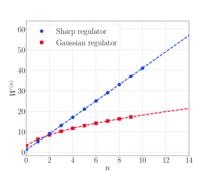
Figure 4: EFT at N²LO. The permissible values of the LEC $C_{22}$ as a function of the cutoff - shaded area. Vertical dashed line - the highest cutoff reproducing $r_{\text{eff}}$ at N²LO. The LECs $C_{0},C_{2},C_{4}$ are fitted to reporduce the Volkov potential $a_{s},r_{\text{eff}},S_{2}$.

Trying the behavior of the theory near the edge of the permissible $C_{22}$ range, we explored the relations between $C_{22}$ and the other LECs. It appears that at the edge of the $C_{22}$ region the LECs possess a singular point, i.e. the renormalization conditions for $C_{0}(C_{22}),C_{2}(C_{22}),C_{4}(C_{22})$ diverge. It follows that as the freedom in $C_{22}$ decreases, the relations between the LECs become more radical. To illustrate this point we plot in Fig. 5 the LEC $C_{0}$ as a function of $C_{22}$ for different cutoffs.

Figure 5: The LEC $C_{0}$ as a function of ${c}_{22}$ at differect cutoffs. The scattering parameters $a_{s},r_{\text{eff}},S_{2}$ are constrained by the Volkov potential. Blue (full) line - $\Lambda=1.0\;\text{fm}^{-1}$, red (dashed) line - $\Lambda=1.5\;\text{fm}^{-1}$, purple (dashed-dot) line - $\Lambda=2.0\;\text{fm}^{-1}$, and green (dotted) line - $\Lambda=2.5\;\text{fm}^{-1}$.

The shrinking of the permissible $C_{22}$ interval in the limit $\Lambda\longrightarrow\Lambda^{(2)}_{\text{max}}$ may lead us to think that in this limit $C_{22}$ becomes redundant. That is, the range of possible predictions implied from the freedom in $C_{22}$ should shrink as well. To check this hypothesis we have utilized our EFT to calculate the triton’s binding energy $E_{3}(\text{Volkov})$, that for the Volkov potential is equal to $-8.431\,\text{MeV}$. The results of these calculations are presented in Fig. 6 as a function of $\Lambda$. Surprisingly, we have found that up to rather high values of $\Lambda$ the $E_{3}(C_{22})$ range increases while the permissible interval of $C_{22}$ decreases. At low cutoffs, the upper bound on $E_{3}$ coincides with the 2-body threshold, and it decreases slowly as $\Lambda\longrightarrow\Lambda^{(2)}_{\text{max}}$. In contrast, the lower bound drops dramatically, following the standard path of the Thomas collapse Thomas1935a up to $\Lambda\approx 2.7\,\text{fm}^{-1}$. Above this point the collapse stops, and near the critical point $\Lambda\approx\Lambda^{(2)}_{\text{max}}$ the values of $E_{3}$ become comparable to the exact binding energy $E_{3}(\text{Volkov})$.

Figure 6: The triton’s binding energy $E_{3}$ as a function of the cutoff. Blue line - the exact value for the Volkov potential. Shaded gray area - range of possible EFT (at N²LO) predictions, reflecting the permissible values of $C_{22}$, see Fig. 4.

To better understand this result and its consequences, we have calculated the triton’s binding energy also at LO, and NLO, see Fig. 7. From the figure it can be seen that if the LO calculations are performed at $\Lambda=\Lambda^{(0)}_{\max}$, reproducing $r_{\text{eff}}$, the resulting $E_{3}(\text{LO})$ is rather close to $E_{3}(\text{Volkov})$. For NLO this point is extended into a range over which $E_{3}(\text{NLO})\approx E_{3}(\text{Volkov})$, but as $\Lambda\to\Lambda^{(1)}_{\max}$ the energy deviates and at the critical point $E_{3}\approx-5~{}\text{MeV}$. We note that at N²LO we can renormalization $C_{22}$ to reproduce $E_{3}(\text{Volkov})$, thus eliminating the 3-body force. This we can do up to about $\Lambda=3~{}\text{fm}^{-1}$, the point where the exact result is excluded from the permissible $E_{3}$ region. From this point on $E_{3}$ will move along the lower bound of the region until at $\Lambda^{(2)}_{\max}$ it will reach a value $E_{3}\approx-5~{}\text{MeV}$. Following a pattern similar to NLO.

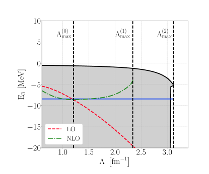
Figure 7: The triton’s binding energy $E_{3}$ as a function of the cutoff, like in Fig. 6, with the addition of the LO, and NLO results.

V Summary

For a non-perturbative contact EFT we analyzed the evolution of the Wigner bound parameter $W^{(n)}$ with the EFT order $n$. Considering sharp and Gaussian regulators, we have found, up to $n=10$ and $n=9$ respectively, an analytic lower limit for $W^{(n)}$. This limit is regulator specific. From this analysis, we have concluded that the Wigner bound loosens with increasing EFT order, and conjectured for these regulators the general dependence of $W^{(n)}$ on $n$. If holds, this conjecture implies that $W^{(n)}$ diverge in the limit $n\to\infty$ defeating the Wigner bound, and restoring renormalization group invariance for a complete theory.

Verifying our results with a concrete numerical example we have demonstrated at N²LO that our conclusions hold after full renormalization procedure, as long as at least one LEC is utilized to maximize the cutoff. Studying the 3-body system with this example, we have found that limiting the permissible range of cutoffs by the Wigner bound, we avoid the Thomas collapse, and don’t need to promote the 3-body force to LO. If proven for the general case this observation might be of practical importance, as a 3-body force appearing at LO, and 4-body force appearing at NLO, are a huge liability from a computational many-body perspective.

The implications of the current observation on the nuclear $\not{\pi}$EFT , on $p$-wave interaction, and on $\chi$EFT call for further study.

- (1) R. Higa, H.-W. Hammer, U. van Kolck, scattering in halo effective field theory, Nucl. Phys. A 809, 171 (2008).
- (2) E. Braaten, H.-W. Hammer, Universality in few-body systems with large scattering length, Phys. rep. 428, 259 (2006).
- (3) H.-W. Hammer, C. Ji, and D. R. Phillips, Effective field theory description of halo nuclei, J. Phys. G 44, 103002 (2017).
- (4) H. W. Hammer, S. könig, U. van Kolck, Nuclear effective field theory: status and perspectives, arXiv:nucl-th/1906.12122 (2019).
- (5) P. Lepage, How to Renormalize the Schrodinger Equation, arXiv:nucl-th/9706029 (1997).
- (6) P. F. Bedaque, U. van Kolck, Effective field theory for few nucleon systems, Ann. Rev. Nuc. 52, 339 (2002).
- (7) S. R. Beane, P.-F. Bedaque, W. C. Haxton, D. R. Phillips, M. J. Savage, From Hadrons to Nuclei: Crossing the Border, In At the frontier of particle physics, edited by M. Shifman (World Scientific, 2001) vol. 1 p. 133.
- (8) D. B. Kaplan, Five lectures on effective field theory, arXiv:nucl-th/0510023 (2005).
- (9) E. Epelbaum, J. Gegelia, U. Meißner, Wilsonian renormalization group versus subtractive renormalization in effective field theories for nucleon–nucleon scattering, Nucl. Phys. B 925, 161 (2017).
- (10) M. Pavón Valderrama, Power counting and Wilsonian renormalization in nuclear effective field theory, Int. J. Mod. Phys. 25, 1641007 (2016).
- (11) P. F. Bedaque, H.-W. Hammer, and U. van Kolck, Renormalization of the Three-Body System with Short-Range Interactions, Phys. Rev. Lett. 82, 463 (1999).
- (12) B. Bazak, J. Kirscher, S. König, M. P. Valderrama, N. Barnea, and U. van Kolck, Four-Body Scale in Universal Few-Boson Systems, Phys. Rev. Lett. 122, 143001 (2019).
- (13) S. Weinberg, Nuclear forces from chiral lagrangians, Phys. Lett. B 251, 288 (1990).
- (14) D. R. Phillips and T. D. Cohen, How short is too short? Constraining zero-range interactions in nucleon-nucleon scattering, Phys. Lett. B 390, 7 (1997).
- (15) D. R. Phillips, S. R. Beane, and T. D. Cohen, Non-perturbative regularization and renormalization: simple examples from non-relativistic quantum mechanics, Ann. Phys. 263, 255 (1998).
- (16) E. P. Wigner, Lower Limit for the Energy Derivative of the Scattering Phase Shift, Phys. Rev. 98, 145 (1955).
- (17) H. W. Hammer and D. Lee, Causality and the effective range expansion, Ann. Phys. 325, 2212 (2010).
- (18) S. R. Beane, T. D. Cohen, and D. R. Phillips, The potential of effective field theory in NN scattering, Nucl. Phys. A 632, 445 (1998).
- (19) U. van Kolck, Effective field theory of short-range forces, Nucl. Phys. A 645, 273 (1999).
- (20) A. Bansal, S. Binder, A. Ekström, G. Hagen, G. R. Jansen, and T. Papenbrock, Pion-less effective field theory for atomic nuclei and lattice nuclei, Phys. Rev. C 98, 054301 (2018).
- (21) V. Lensky, M. C. Birse, and N. R. Walet, Description of light nuclei in pionless effective field theory using the stochastic variational method, Phys. Rev. C 94, 034003 (2016).
- (22) E. Epelbaum, A. M. Gasparyan, J. Gegelia, and U.-G. Meißner, How (not) to renormalize integral equations with singular potentials in effective field theory, Euro. Phys. J. A 54, 186 (2018).
- (23) C. Arzt, Reduced effective Lagrangians Phys. Lett. B 342 189 (1995)
- (24) S. R. Beane, M. J. Savage, Rearranging pionless effective field theory, Nucl. Phys. A 694, 511 (2001).
- (25) L. H. Thomas, The Interaction Between a Neutron and a Proton and the Structure of H3, Phys. Rev. 47, 903 (1935).
- (26) V. N. Efimov, Energy levels arising form the resonant two-body forces in a three-body system, Phys. Lett. B 33, 563 (1970).