USTC-ICTS-19-16 Modular $A_{4}$ Symmetry Models of Neutrinos and Charged Leptons

Abstract

We present a comprehensive analysis of neutrino mass and lepton mixing in theories with $A_{4}$ modular symmetry, where the only flavon field is the single modulus field $\tau$, and all masses and Yukawa couplings are modular forms. Similar to previous analyses, we discuss all the simplest neutrino sectors arising from both the Weinberg operator and the type I seesaw mechanism, with lepton doublets and right-handed neutrinos assumed to be triplets of $A_{4}$. Unlike previous analyses, we allow right-handed charged leptons to transform as all combinations of $\mathbf{1}$, $\mathbf{1}^{\prime}$ and $\mathbf{1}^{\prime\prime}$ representations of $A_{4}$, using the simplest different modular weights to break the degeneracy, leading to ten different charged lepton Yukawa matrices, instead of the usual one. This implies ten different Weinberg models and thirty different type I seesaw models, which we analyse in detail. We find that fourteen models for both NO and IO neutrino mass ordering can accommodate the data, as compared to one in previous analyses, providing many new possibilities.

1 Introduction

Despite the measurement of a non-zero reactor angle, it remains an intriguing possibility that the large mixing angles in the lepton sector can be explained using some discrete non-Abelian family symmetry [1, 2]. The origin of such a symmetry could either be a continuous non-Abelian gauge symmetry, broken to a discrete subgroup [3, 4, 5, 6, 7, 8, 9], or it could emerge from extra dimensions [10, 11, 12, 13, 14, 15, 16, 17, 18, 19, 20, 21], either as an accidental symmetry of the orbifold fixed points, or as a subgroup of the symmetry of the extra dimensional lattice vectors, commonly referred to as modular symmetry [22, 23, 24].

Recently it has been suggested that neutrino masses might be modular forms [25], with constraints on the Yukawa couplings. The idea is that, since modular invariance controls orbifold compactifications of the heterotic superstring, this implies that the 4d effective Lagrangian must respect modular symmetry, hence the Yukawa couplings (involving twisted states whose modular weights do not add up to zero) are modular forms [25]. Hence the Yukawa couplings form multiplets with well defined alignments, prescribed by the modular form, which depend on a single complex modulus field $\tau$.

This has led to a revival of the idea that modular symmetries are symmetries of the extra dimensional spacetime with Yukawa couplings determined by their modular weights [25, 26]. The finite modular subgroups considered in the literature include $\Gamma(2)$ [27, 28, 29, 30], $\Gamma(3)$ [25, 26, 27, 31, 32, 28, 33, 34], $\Gamma(4)$ [35, 36, 37] and $\Gamma(5)$ [38, 39]. The $\Gamma(3)$ case has been applied to grand unified theories with the modulus fixed by the orbifold construction [40]. The formalism with a single complex modulus field $\tau$ has also been extended to the case of multiple moduli fields $\tau_{i}$ [41]. The generalized CP symmetry in modular invariant models are studied in [42]. The formalism of modular invariant approach has extended to include odd weight modular forms [43].

In this paper, we shall study the finite modular group $\Gamma_{3}\cong A_{4}$ with a single modulus field $\tau$ and no other flavons, hence all masses and Yukawa couplings are modular forms. Similar to previous analyses [25, 26, 31, 32, 28, 27, 33, 34], we discuss all the simplest neutrino sectors arising from both the Weinberg operator and the type I seesaw mechanism, with lepton doublets and right-handed neutrinos assumed to be triplets of $A_{4}$. However, unlike all previous analyses [25, 26, 31, 32, 28, 27, 33, 34], we allow right-handed charged leptons to transform as all combinations of $\mathbf{1}$, $\mathbf{1}^{\prime}$ and $\mathbf{1}^{\prime\prime}$ representations of $A_{4}$, using the simplest different modular weights to break the degeneracy, leading to ten different charged lepton Yukawa matrices, instead of the usual one. This implies ten different Weinberg models and thirty different type I seesaw models, which we analyse in detail. We find that fourteen models for both normal ordering (NO) and inverted ordering (IO) neutrino mass spectrums can accommodate the data, as compared to one in previous analyses, providing many new possibilities.

The structure of the paper is as follows. In section 2 we briefly outline the idea of modular symmetry, and we specialize to $\Gamma(3)$ modular symmetry and give the modular forms of level $N=3$. Then in section 3 we systematically construct and classify the forty simplest models based on $\Gamma_{3}\cong A_{4}$, generalising previous analyses in the charged lepton sector as outlined above. After that in section 4 we perform a comprehensive and systematic numerical analysis for each of the forty models discussed in the previous section, giving the best fit values of the parameters for each viable model with NO and the corresponding predictions in a detailed compendium of tables and figures. Section 5 concludes the paper.

2 Modular symmetry and modular forms of level $N=3$

In the following, we briefly review the modular symmetry and the its congruence subgroups. The special linear group $SL(2,\mathbb{Z})$ is constituted by $2\times 2$ matrices with integer entries and determinant 1 [44, 45]:

$$SL(2,\mathbb{Z})=\left\{\left(\begin{array}[]{cc}a&b\\ c&d\end{array}\right)\bigg{|}a,b,c,d\in\mathbb{Z},ad-bc=1\right\}\,.$$ (1)

The upper half plane, denoted as $\mathcal{H}$, is the set of all complex numbers with positive imaginary part: $\mathcal{H}=\left\{\tau\in\mathbb{C}~{}|~{}\Im\tau>0\right\}$. The $SL(2,\mathbb{Z})$ group acts on $\mathcal{H}$ via fractional linear transformations (or M$\ddot{\mathrm{o}}$bius transformations),

$$\gamma=\begin{pmatrix}a&b\\ c&d\end{pmatrix}:\mathcal{H}\rightarrow\mathcal{H},\quad\tau\mapsto\gamma\tau=\gamma(\tau)=\frac{a\tau+b}{c\tau+d}\,.$$ (2)

It is straightforward to check that

$$\Im(\gamma(\tau))=\frac{\Im\tau}{|c\tau+d|^{2}},\quad\gamma=\begin{pmatrix}a&b\\ c&d\end{pmatrix}\in SL(2,\mathbb{Z})\,,$$ (3)

which implies if $\gamma\in SL(2,\mathbb{Z})$ and $\tau\in\mathcal{H}$ then also $\gamma(z)\in\mathcal{H}$. Therefore the modular group maps the upper half plane back to itself. In fact the modular group acts on the upper half plane, meaning that $I(\tau)=\tau$ where $I$ is the $2\times 2$ identity matrix and $(\gamma\gamma^{\prime})(\tau)=\gamma(\gamma^{\prime}(\tau))$ for any $\gamma,\gamma^{\prime}\in SL(2,\mathbb{Z})$ and $\tau\in\mathcal{H}$. Furthermore, $\gamma$ and $-\gamma$ evidently give the same action, therefore it is more natural to consider the projective special linear group $PSL(2,\mathbb{Z})=SL(2,\mathbb{Z})/\{I,-I\}$, the quotient of $SL(2,\mathbb{Z})$ by $\pm I$. The group $PSL(2,\mathbb{Z})$ is usually called the modular group in the literature, and it can be generated by two elements $S$ and $T$ [44]

$$S=\left(\begin{array}[]{cc}0{}&~{}1\\ -1{}&~{}0\end{array}\right),\quad T=\left(\begin{array}[]{cc}1{}&~{}1\\ 0{}&~{}1\end{array}\right)\,,$$ (4)

which satisfy the relations

$$S^{2}=(ST)^{3}=\mathds{1}\,.$$ (5)

The actions of $S$ and $T$ on $\mathcal{H}$ are given by

$$S:\tau\mapsto-\frac{1}{\tau},\qquad T:\tau\mapsto\tau+1\,.$$ (6)

For a positive integer $N$, the principal congruence subgroup of level $N$ of is defined as

$$\Gamma(N)=\left\{\left(\begin{array}[]{cc}a&b\\ c&d\end{array}\right)\in SL(2,\mathbb{Z}),~{}~{}a\equiv d\equiv 1~{}({\tt mod}~{}N),~{}~{}b\equiv c\equiv 0~{}({\tt mod}~{}N)\right\}\,,$$ (7)

which is a normal subgroup of the special linear group $SL(2,\mathbb{Z})$. Obviously $\Gamma(1)\cong SL(2,\mathbb{Z})$ is the special linear group. It is easy to obtain

$$T^{N}=\begin{pmatrix}1~{}&~{}N\\ 0~{}&~{}1\end{pmatrix}\,,$$ (8)

which implies $T^{N}\in\Gamma(N)$, i.e., $T^{N}$ is an element of $\Gamma(N)$. Taking the quotient of $\Gamma(1)$ and $\Gamma(2)$ by $\{I,-I\}$, we obtain the projective principal congruence subgroups $\overline{\Gamma}(N)=\Gamma(N)/\{I,-I\}$ for $N=1,2$, and $\overline{\Gamma}(N>2)=\Gamma(N)$ since the element $-I$ doesn’t belong to $\Gamma(N)$ for $N>2$. The quotient groups $\Gamma_{N}=\overline{\Gamma}(1)/\overline{\Gamma}(N)$ are usually called finite modular groups, and the group $\Gamma_{N}$ can be obtained from $\overline{\Gamma}(1)$ by imposing the condition $T^{N}=1$. Consequently the generators $S$ and $T$ of $\Gamma_{N}$ satisfy the relations

$$S^{2}=(ST)^{3}=T^{N}=\mathds{1}\,.$$ (9)

The groups $\Gamma_{N}$ with $N=2$, $3$, $4$, $5$ are isomorphic to the permutation groups $S_{3}$, $A_{4}$, $S_{4}$ and $A_{5}$ respectively [24].

The crucial element of modular invariance approach is the modular form $f(\tau)$ of weight $k$ and level $N$. The modular form $f(\tau)$ is a holomorphic function of the complex modulus $\tau$ and it is required to satisfy the following modular transformation property under the group $\Gamma(N)$,

$$f\left(\frac{a\tau+b}{c\tau+d}\right)=(c\tau+d)^{k}f(\tau)\quad\text{for}\quad\forall~{}~{}\gamma=\begin{pmatrix}a&b\\ c&d\end{pmatrix}\in\Gamma(N)~{}~{}\text{and}~{}~{}\tau\in\mathcal{H}\,.$$ (10)

The modular forms of weight $k$ and level $N$ span a linear space $\mathcal{M}_{k}(\Gamma(N))$ with finite dimension. As has been shown in [25, 43], we can choose the basis vectors of $\mathcal{M}_{k}(\Gamma(N))$ such that they can be organized into multiplets of modular forms $F_{\mathbf{r}}(\tau)\equiv\left(f_{1}(\tau),\,f_{2}(\tau),\,\dots\right)^{T}$ which transform in certain irreducible representation of the finite modular group $\Gamma_{N}$,

$$F_{\mathbf{r}}(\gamma\tau)=(c\tau+d)^{k}\rho_{\mathbf{r}}(\gamma)F_{\mathbf{r}}(\tau),\quad\gamma\in\overline{\Gamma}(1)\,,$$ (11)

where $\gamma$ is the representative element of the coset $\gamma\overline{\Gamma}(N)$ in $\Gamma_{N}$, and $\rho_{\mathbf{r}}(\gamma)$ is the representation matrix of the element $\gamma$ in the irreducible representation $\mathbf{r}$. When $\gamma$ is the generators $S$ and $T$, Eq. (11) gives

$$F_{\mathbf{r}}(S\tau)=\tau^{k}\rho_{\mathbf{r}}(S)F_{\mathbf{r}}(\tau),\quad F_{\mathbf{r}}(T\tau)=\rho_{\mathbf{r}}(T)F_{\mathbf{r}}(\tau)\,,$$ (12)

for even $k$.

2.1 Modular forms of level $N=3$

In the present work, we present a comprehensive analysis of neutrino mass and lepton mixing in theories with $\Gamma(3)$ modular symmetry. The finite modular group $\Gamma_{3}$ is isomorphic to $A_{4}$ which is the symmetry group of the tetrahedron. It contains twelve elements and it is the smallest non-abelian finite group which admits a three-dimensional irreducible representation. The $A_{4}$ group has three singlet representations $\mathbf{1}$, $\mathbf{1}^{\prime}$, $\mathbf{1}^{\prime\prime}$ and a triplet representation $\mathbf{3}$. In the singlet representations, we have

$$\mathbf{1}:~{}~{}S=1,\qquad T=1\,,$$ (13)

$$\mathbf{1}^{\prime}:~{}~{}S=1,\qquad T=\omega^{2}\,,$$

$$\mathbf{1}^{\prime\prime}:~{}~{}S=1,\qquad T=\omega\,,$$

with $\omega=e^{2\pi i/3}=-1/2+i\sqrt{3}/2$. For the representation $\mathbf{3}$, we will choose a basis in which the generator $T$ is diagonal. The explicit forms of $S$ and $T$ are

$$S=\frac{1}{3}\begin{pmatrix}-1&2&2\\ 2&-1&2\\ 2&2&-1\end{pmatrix},~{}\quad~{}T=\begin{pmatrix}1~{}&~{}0~{}&~{}0\\ 0~{}&~{}\omega^{2}~{}&~{}0\\ 0~{}&~{}0~{}&~{}\omega\end{pmatrix}\,,$$ (14)

The basic multiplication rule is

$$\mathbf{3}\otimes\mathbf{3}=\mathbf{1}\oplus\mathbf{1^{\prime}}\oplus\mathbf{1^{\prime\prime}}\oplus\mathbf{3}_{S}\oplus\mathbf{3}_{A}\,,$$ (15)

where the subscripts $S$ and $A$ denotes symmetric and antisymmetric combinations respectively. If we have two triplets $\alpha=(\alpha_{1},\alpha_{2},\alpha_{3})\sim\mathbf{3}$ and $\beta=(\beta_{1},\beta_{2},\beta_{3})\sim\mathbf{3}$, we can obtain the following irreducible representations from their product,

$$(\alpha\beta)_{\mathbf{1}}=\alpha_{1}\beta_{1}+\alpha_{2}\beta_{3}+\alpha_{3}\beta_{2}\,,$$

$$(\alpha\beta)_{\mathbf{1}^{\prime}}=\alpha_{3}\beta_{3}+\alpha_{1}\beta_{2}+\alpha_{2}\beta_{1}\,,$$

$$(\alpha\beta)_{\mathbf{1}^{\prime\prime}}=\alpha_{2}\beta_{2}+\alpha_{1}\beta_{3}+\alpha_{3}\beta_{1}\,,$$

$$(\alpha\beta)_{\mathbf{3}_{S}}=(2\alpha_{1}\beta_{1}-\alpha_{2}\beta_{3}-\alpha_{3}\beta_{2},2\alpha_{3}\beta_{3}-\alpha_{1}\beta_{2}-\alpha_{2}\beta_{1},2\alpha_{2}\beta_{2}-\alpha_{1}\beta_{3}-\alpha_{3}\beta_{1})\,,$$

$$(\alpha\beta)_{\mathbf{3}_{A}}=(\alpha_{2}\beta_{3}-\alpha_{3}\beta_{2},\alpha_{1}\beta_{2}-\alpha_{2}\beta_{1},\alpha_{3}\beta_{1}-\alpha_{1}\beta_{3})\,.$$ (16)

The linear space of the modular forms of integral weight $k$ and level $N=3$ has dimension $k+1$ [46, 25]. The modular space $\mathcal{M}_{2k}(\Gamma(3))$ can be constructed from the Dedekind eta-function $\eta(\tau)$ which is defined as

$$\eta(\tau)=q^{1/24}\prod_{n=1}^{\infty}(1-q^{n}),\qquad q=e^{2\pi i\tau}\,.$$ (17)

The eta function $\eta(\tau)$ satisfies the following identities

$$\eta(\tau+1)=e^{i\pi/12}\eta(\tau),\qquad\eta(-1/\tau)=\sqrt{-i\tau}~{}\eta(\tau)\,.$$ (18)

There are only three linearly independent modular forms of weight 2 and level 3, which are denoted as $Y_{i}(\tau)$ with $i=1,2,3$. We can arrange the three modular functions into a vector $Y^{(2)}_{\mathbf{3}}=\left(Y_{1},Y_{2},Y_{3}\right)^{T}$ transforming as a triplet $\mathbf{3}$ of $A_{4}$. The modular forms $Y_{i}$ can be expressed in terms of $\eta(\tau)$ and its derivative as follow [25]:

$$Y_{1}(\tau) = \frac{i}{2\pi}\left[\frac{\eta^{\prime}(\tau/3)}{\eta(\tau/3)}+\frac{\eta^{\prime}((\tau+1)/3)}{\eta((\tau+1)/3)}+\frac{\eta^{\prime}((\tau+2)/3)}{\eta((\tau+2)/3)}-\frac{27\eta^{\prime}(3\tau)}{\eta(3\tau)}\right],$$

$$Y_{2}(\tau) = \frac{-i}{\pi}\left[\frac{\eta^{\prime}(\tau/3)}{\eta(\tau/3)}+\omega^{2}\frac{\eta^{\prime}((\tau+1)/3)}{\eta((\tau+1)/3)}+\omega\frac{\eta^{\prime}((\tau+2)/3)}{\eta((\tau+2)/3)}\right],$$

$$Y_{3}(\tau) = \frac{-i}{\pi}\left[\frac{\eta^{\prime}(\tau/3)}{\eta(\tau/3)}+\omega\frac{\eta^{\prime}((\tau+1)/3)}{\eta((\tau+1)/3)}+\omega^{2}\frac{\eta^{\prime}((\tau+2)/3)}{\eta((\tau+2)/3)}\right]\,.$$ (19)

Notice that $12\eta^{\prime}(\tau)/\eta(\tau)\equiv i\pi E_{2}(\tau)$, where $E_{2}(\tau)$ is the well-known Eisenstein series of weight 2 [44]. The $q$-expansions of the triplet modular forms $Y^{(2)}_{\mathbf{3}}$ are given by

$$Y^{(2)}_{\mathbf{3}}=\begin{pmatrix}Y_{1}(\tau)\\ Y_{2}(\tau)\\ Y_{3}(\tau)\end{pmatrix}=\begin{pmatrix}1+12q+36q^{2}+12q^{3}+84q^{4}+72q^{5}+\dots\\ -6q^{1/3}(1+7q+8q^{2}+18q^{3}+14q^{4}+\dots)\\ -18q^{2/3}(1+2q+5q^{2}+4q^{3}+8q^{4}+\dots)\end{pmatrix}\,.$$ (20)

They satisfy the constraint [25, 43]

$$(Y^{(2)}_{\mathbf{3}}Y^{(2)}_{\mathbf{3}})_{\mathbf{1}^{\prime\prime}}=Y_{2}^{2}+2Y_{1}Y_{3}=0\,.$$ (21)

Multiplets of higher weight modular forms can be constructed from the tensor products of $Y^{(2)}_{\mathbf{3}}$. Using the $A_{4}$ contraction rule $\mathbf{3}\otimes\mathbf{3}=\mathbf{1}\oplus\mathbf{1^{\prime}}\oplus\mathbf{1^{\prime\prime}}\oplus\mathbf{3}_{S}\oplus\mathbf{3}_{A}$, we can obtain five independent weight 4 modular forms,

$$Y^{(4)}_{\mathbf{3}} = (Y^{(2)}_{\mathbf{3}}Y^{(2)}_{\mathbf{3}})_{\mathbf{3}}=(Y_{1}^{2}-Y_{2}Y_{3},Y_{3}^{2}-Y_{1}Y_{2},Y_{2}^{2}-Y_{1}Y_{3})^{T}\,,$$

$$Y^{(4)}_{\mathbf{1}} = (Y^{(2)}_{\mathbf{3}}Y^{(2)}_{\mathbf{3}})_{\mathbf{1}}=Y_{1}^{2}+2Y_{2}Y_{3}\,,$$

$$Y^{(4)}_{\mathbf{1}^{\prime}} = (Y^{(2)}_{\mathbf{3}}Y^{(2)}_{\mathbf{3}})_{\mathbf{1}^{\prime}}=Y_{3}^{2}+2Y_{1}Y_{2}\,.$$ (22)

Similarly there are seven modular forms of weight 6, and they decompose into a singlet $\mathbf{1}$ and two triplets $\mathbf{3}$ under $A_{4}$,

$$Y^{(6)}_{\mathbf{1}} = (Y^{(2)}_{\mathbf{3}}Y^{(4)}_{\mathbf{3}})_{\mathbf{1}}=Y_{1}^{3}+Y_{2}^{3}+Y_{3}^{3}-3Y_{1}Y_{2}Y_{3}\,,$$

$$Y^{(6)}_{\mathbf{3},1} = Y^{(2)}_{\mathbf{3}}Y^{(4)}_{\mathbf{1}}=(Y_{1}^{3}+2Y_{1}Y_{2}Y_{3},Y_{1}^{2}Y_{2}+2Y_{2}^{2}Y_{3},Y_{1}^{2}Y_{3}+2Y_{3}^{2}Y_{2})^{T}\,,$$

$$Y^{(6)}_{\mathbf{3},2} = Y^{(2)}_{\mathbf{3}}Y^{(4)}_{\mathbf{1}^{\prime}}=(Y_{3}^{3}+2Y_{1}Y_{2}Y_{3},Y_{3}^{2}Y_{1}+2Y_{1}^{2}Y_{2},Y_{3}^{2}Y_{2}+2Y_{2}^{2}Y_{1})^{T}\,.$$ (23)

Notice that $(Y^{(2)}_{\mathbf{3}}Y^{(2)}_{\mathbf{3}})_{\mathbf{1}^{\prime\prime}}$ is vanishing as shown in Eq.(21).

3 Neutrino mass models based on $\Gamma_{3}$ modular symmetry

In this section, we shall perform a systematical classification of all minimal neutrino mass models with the $\Gamma_{3}$ modular symmetry. We adopt the $N=1$ global supersymmetry, the most general form of the action can be written as [25]

$$\mathcal{S}=\int d^{4}xd^{2}\theta d^{2}\bar{\theta}K(\Phi_{I},\bar{\Phi}_{I};\tau,\bar{\tau})+\int d^{4}xd^{2}\theta W(\Phi_{I},\tau)+\mathrm{h.c.}\,,$$ (24)

where $K(\Phi_{I},\bar{\Phi}_{I},\tau,\bar{\tau})$ is the K$\ddot{\mathrm{a}}$hler potential, and $W$ denotes the superpotential. $\Phi_{I}$ is set of chiral superfields, under the modular transformation of Eq. (2), it transforms as

$$\tau\to\gamma\tau=\frac{a\tau+b}{c\tau+d}\,,\qquad\Phi_{I}\to(c\tau+d)^{-k_{I}}\rho_{I}(\gamma)\Phi_{I}\,.$$ (25)

where $-k_{I}$ is the modular weight, and $\rho_{I}(\gamma)$ is the unitary representation of the representative element $\gamma$ in $\Gamma_{N}$. There are no restrictions on the possible value of $k_{I}$ since the supermultiplets $\Phi_{I}$ are not modular forms. The K$\ddot{\mathrm{a}}$hler potential should be invariant up to K$\ddot{\mathrm{a}}$hler transformations under the modular transformation of Eq. (25). We shall use the following K$\ddot{\mathrm{a}}$hler potential in this work [25],

$$K(\Phi_{I},\bar{\Phi}_{I};\tau,\bar{\tau})=-h\log(-i\tau+i\bar{\tau})+\sum_{I}(-i\tau+i\bar{\tau})^{-k_{I}}|\Phi_{I}|^{2}~{}~{}~{},$$ (26)

where $h$ is a positive constant $h>0$. After the modulus $\tau$ gets a vacuum expectation value (VEV), the above K$\ddot{\mathrm{a}}$hler potential leads to the following kinetic term for the scalar components of the supermultiplets $\Phi_{I}$ and the modulus superfield $\tau$,

$$\frac{h}{\langle-i\tau+i\bar{\tau}\rangle^{2}}\partial_{\mu}\bar{\tau}\partial^{\mu}\tau+\sum_{I}\frac{\partial_{\mu}\bar{\phi}_{I}\partial^{\mu}\phi_{I}}{\langle-i\tau+i\bar{\tau}\rangle^{k_{I}}}\,.$$ (27)

For a given value of the VEV of $\tau$, the kinetic term of $\phi_{I}$ can be made into canonical form by rescaling the fields $\phi_{I}$. This effect can be absorbed into the unknown free parameters of the superpotential in a specific model.

The superpotential $W(\Phi_{I},\tau)$ can be expanded in power series of the involved supermultiplets $\Phi_{I}$,

$$W(\Phi_{I},\tau)=\sum_{n}Y_{I_{1}...I_{n}}(\tau)~{}\Phi_{I_{1}}...\Phi_{I_{n}}\,,$$ (28)

where $Y_{I_{1}...I_{n}}$ is a modular multiplet of weight $k_{Y}$ and it transforms as the presentation $\rho_{Y}$ of $\Gamma_{N}$,

$$\tau\to\gamma\tau=\dfrac{a\tau+b}{c\tau+d}\,,\qquad Y(\tau)\to Y(\gamma\tau)=(c\tau+d)^{k_{Y}}\rho_{Y}(\gamma)Y(\tau)\,.$$ (29)

The requirement of modular invariance of the superpotential implies

$$k_{Y}=k_{I_{1}}+...+k_{I_{n}},~{}\quad~{}\rho_{Y}\otimes\rho_{I_{1}}\otimes\ldots\otimes\rho_{I_{n}}\ni\mathbf{1}\,.$$ (30)

Then we proceed to discuss all possible simplest models for lepton masses and mixing with the $A_{4}$ modular symmetry. In order to construct models with the smallest number of free parameters, we don’t introduce any flavon field other than the modulus $\tau$. The Higgs doublets $H_{u}$ and $H_{d}$ are assumed to transform as $\mathbf{1}$ under $A_{4}$ and their modular weights $k_{H_{u},H_{d}}$ are vanishing. We consider two scenarios where the neutrino masses arise from the Weinberg operator and the type I seesaw mechanism. Similar to previous analyses [25], we assign the three generations of left-handed lepton doublets $L\equiv(L_{1},L_{2},L_{3})^{T}$ and of the right-handed neutrino $N^{c}\equiv(N^{c}_{1},N^{c}_{2},N^{c}_{3})^{T}$ to two triplets $\mathbf{3}$ of $A_{4}$ with modular weights denoted as $k_{L}$ and $k_{N^{c}}$. Unlike previous work [25, 26, 31, 32, 28, 27, 33, 34], we allow right-handed charged leptons $E^{c}_{1,2,3}$ to transform as all combinations of $\mathbf{1}$, $\mathbf{1}^{\prime}$ and $\mathbf{1}^{\prime\prime}$ representations of $A_{4}$, using the simplest different modular weights $k_{E_{1,2,3}}$ to break the degeneracy, leading to ten different charged lepton Yukawa matrices, instead of the usual one.

3.1 Charged lepton sector

Firstly we investigate the charged lepton sector. Since we do not allow any flavons (beyond the single modulus field $\tau$), we shall not attempt to explain the charged lepton mass hierarchy, which remains a challenge for modular symmetry models. In order to avoid a charged lepton mass matrix with rank less than 3, when two or all of $E^{c}_{1},\,E^{c}_{2}$ and $E^{c}_{3}$ have same representation of $\Gamma_{3}$ , we assume that $E^{c}_{1},\,E^{c}_{2}$ and $E^{c}_{3}$ have different modular weights such that they are distinguishable. For simplicity, we use lower weight modular forms as much as possible. Hence the model in the charged lepton sector can be divided into three possible cases.

• $\rho_{E^{c}_{1}}=\rho_{E^{c}_{2}}=\rho_{E^{c}_{3}}$

  When all the three right-handed charged leptons $E^{c}_{1,2,3}$ transform as the same irreducible representation of $\Gamma_{3}$, they should carry different modular weights to distinguish from each other. As a consequence, the charged leptons $E^{c}_{1,2,3}$ could couple with the modular forms $Y^{(2)}_{\mathbf{3}}$, $Y^{(4)}_{\mathbf{3}}$ and $Y^{(6)}_{\mathbf{3}}$ respectively, and the superpotential for the charged lepton masses can be written as:

  $$W_{e}\,=\alpha(E^{c}_{1}LY^{(2)}_{\mathbf{3}})_{\mathbf{1}}H_{d}+\beta(E^{c}_{2}LY^{(4)}_{\mathbf{3}})_{\mathbf{1}}H_{d}+\gamma(E^{c}_{3}LY^{(6)}_{\mathbf{3}})_{\mathbf{1}}H_{d}\,.$$ (31)

  The condition of modular invariance requires

  $$k_{E_{1}}=k_{E_{2}}-2=k_{E_{3}}-4=2-k_{L}\,.$$ (32)

• $\rho_{E^{c}_{1}}=\rho_{E^{c}_{2}}\neq\rho_{E^{c}_{3}}$

  If two of the three right-handed charged leptons $E^{c}_{i}$ transform in the same way under $A_{4}$, they could be assigned to different modular weights which are compensated by the lower weight modular forms $Y^{(2)}_{\mathbf{3}}$ and $Y^{(4)}_{\mathbf{3}}$. Thus the superpotential for the charged lepton masses are given by,

  $$W_{e}=\alpha(E^{c}_{1}LY^{(2)}_{\mathbf{3}})_{\mathbf{1}}H_{d}+\beta(E^{c}_{2}LY^{(4)}_{\mathbf{3}})_{\mathbf{1}}H_{d}+\gamma(E^{c}_{3}LY^{(2)}_{\mathbf{3}})_{\mathbf{1}}H_{d}\,,$$ (33)

  where the condition of weight cancellation entails

  $$k_{E_{1}}=k_{E_{2}}-2=k_{E_{3}}=2-k_{L}\,.$$ (34)

• $\rho_{E^{c}_{1}}\neq\rho_{E^{c}_{2}}\neq\rho_{E^{c}_{3}}$

  When the three right-handed charged leptons $E^{c}_{i}$ are assigned to three different singlets $\mathbf{1}$, $\mathbf{1}^{\prime}$ and $\mathbf{1}^{\prime\prime}$ of $A_{4}$ as in previous works [25, 26, 31, 32, 28, 27, 33, 34], their modular weights could be identical, and only the lowest weight modular form $Y^{(2)}_{\mathbf{3}}$ is necessary in the minimal model. Then the superpotential for the charged lepton masses takes the form

  $$W_{e}=\alpha(E^{c}_{1}LY^{(2)}_{\mathbf{3}})_{\mathbf{1}}H_{d}+\beta(E^{c}_{2}LY^{(2)}_{\mathbf{3}})_{\mathbf{1}}H_{d}+\gamma(E^{c}_{3}LY^{(2)}_{\mathbf{3}})_{\mathbf{1}}H_{d}\,.$$ (35)

  The invariance of $W_{e}$ under modular transformations implies the following relations for the weights,

  $$k_{E_{1}}=k_{E_{2}}=k_{E_{3}}=2-k_{L}\,.$$ (36)

To be more specific, making use of the Clebsch-Gordan coefficients given in Eq. (16), we can expand the superpotentials of Eqs. (31, 33, 35) into the following forms for all possible singlet assignments of right-handed charged leptons.

• $\rho_{E^{c}_{1,2,3}}=\mathbf{1},\,k_{E^{c}_{1,2,3}}+k_{L}=2,4,6$

  $$W_{e} =\alpha E^{c}_{1}(LY^{(2)}_{\mathbf{3}})_{\mathbf{1}}H_{d}+\beta E^{c}_{2}(LY^{(4)}_{\mathbf{3}})_{\mathbf{1}}H_{d}+\gamma_{1}E^{c}_{3}(LY^{(6)}_{\mathbf{3},1})_{\mathbf{1}}H_{d}+\gamma_{2}E^{c}_{3}(LY^{(6)}_{\mathbf{3},2})_{\mathbf{1}}H_{d}$$

  $$=\alpha E^{c}_{1}(L_{1}Y_{1}+L_{2}Y_{3}+L_{3}Y_{2})H_{d}$$

  $$\quad+\beta E^{c}_{2}[L_{1}(Y^{2}_{1}-Y_{2}Y_{3})\,+\,L_{2}(Y^{2}_{2}-Y_{1}Y_{3})+L_{3}(Y^{2}_{3}-Y_{1}Y_{2})]H_{d}$$

  $$\quad+\gamma_{1}E^{c}_{3}[L_{1}(Y^{3}_{1}+2Y_{1}Y_{2}Y_{3})\,+\,L_{2}(Y^{2}_{1}Y_{3}+2Y^{2}_{3}Y_{2})\,+\,L_{3}(Y^{2}_{1}Y_{2}+2Y^{2}_{2}Y_{3})]H_{d}$$

  $$\quad+\gamma_{2}E^{c}_{3}[L_{1}(Y^{3}_{3}+2Y_{1}Y_{2}Y_{3})\,+\,L_{2}(Y^{2}_{3}Y_{2}+2Y^{2}_{2}Y_{1})\,+\,L_{3}(Y^{2}_{3}Y_{1}+2Y^{2}_{1}Y_{2})]H_{d}\,.$$ (37)

• $\rho_{E^{c}_{1,2,3}}=\mathbf{1}^{\prime},k_{E^{c}_{1,2,3}}+k_{L}=2,4,6$

  $$W_{e} =\alpha E^{c}_{1}(LY^{(2)}_{\mathbf{3}})_{\mathbf{1}^{\prime\prime}}H_{d}+\beta E^{c}_{2}(LY^{(4)}_{\mathbf{3}})_{\mathbf{1}^{\prime\prime}}H_{d}+\gamma_{1}E^{c}_{3}(LY^{(6)}_{\mathbf{3},1})_{\mathbf{1}^{\prime\prime}}H_{d}+\gamma_{2}E^{c}_{3}(LY^{(6)}_{\mathbf{3},2})_{\mathbf{1}^{\prime\prime}}H_{d}$$

  $$=\alpha E^{c}_{1}(L_{2}Y_{2}+L_{3}Y_{1}+L_{1}Y_{3})H_{d}$$

  $$\quad+\beta E^{c}_{2}[L_{2}(Y^{2}_{3}-Y_{1}Y_{2})\,+\,L_{3}(Y^{2}_{1}-Y_{2}Y_{3})+L_{1}(Y^{2}_{2}-Y_{1}Y_{3})]H_{d}$$

  $$\quad+\gamma_{1}E^{c}_{3}[L_{2}(Y^{2}_{1}Y_{2}+2Y^{2}_{2}Y_{3})\,+\,L_{3}(Y^{3}_{1}+2Y_{1}Y_{2}Y_{3})\,+\,L_{1}(Y^{2}_{1}Y_{3}+2Y^{2}_{3}Y_{2})]H_{d}$$

  $$\quad+\gamma_{2}E^{c}_{3}[L_{2}(Y^{2}_{3}Y_{1}+2Y^{2}_{1}Y_{2})\,+\,L_{3}(Y^{3}_{3}+2Y_{1}Y_{2}Y_{3})\,+\,L_{1}(Y^{2}_{3}Y_{2}+2Y^{2}_{2}Y_{1})]H_{d}\,.$$ (38)

• $\rho_{E^{c}_{1,2,3}}=\mathbf{1}^{\prime\prime},\,k_{E^{c}_{1,2,3}}+k_{L}=2,4,6$

  $$W_{e} =\alpha E^{c}_{1}(LY^{(2)}_{\mathbf{3}})_{\mathbf{1^{\prime}}}H_{d}+\beta E^{c}_{2}(LY^{(4)}_{\mathbf{3}})_{\mathbf{1^{\prime}}}H_{d}+\gamma_{1}E^{c}_{3}(LY^{(6)}_{\mathbf{3},1})_{\mathbf{1^{\prime}}}H_{d}+\gamma_{2}E^{c}_{3}(LY^{(6)}_{\mathbf{3},2})_{\mathbf{1^{\prime}}}H_{d}$$

  $$=\alpha E^{c}_{1}(L_{3}\,Y_{3}+L_{1}\,Y_{2}+L_{2}\,Y_{1})H_{d}$$

  $$\quad+\beta E^{c}_{2}[L_{3}(Y^{2}_{2}-Y_{1}Y_{3})+L_{1}(Y^{2}_{3}-Y_{1}Y_{2})+L_{2}(Y^{2}_{1}-Y_{2}Y_{3})]H_{d}$$

  $$\quad+\gamma_{1}E^{c}_{3}[L_{3}(Y^{2}_{1}Y_{3}+2Y^{2}_{3}Y_{2})+L_{1}(Y^{2}_{1}Y_{2}+2Y^{2}_{2}Y_{3})+L_{2}(Y^{3}_{1}+2Y_{1}Y_{2}Y_{3})]H_{d}$$

  $$\quad+\gamma_{2}E^{c}_{3}[L_{3}(Y^{2}_{3}Y_{2}+2Y^{2}_{2}Y_{1})+L_{1}(Y^{2}_{3}Y_{1}+2Y^{2}_{1}Y_{2})+L_{2}(Y^{3}_{3}+2Y_{1}Y_{2}Y_{3})]H_{d}\,.$$ (39)

• $\rho_{E^{c}_{1,2,3}}=\mathbf{1},\mathbf{1},\mathbf{1}^{\prime}$, $k_{E^{c}_{1,2,3}}+k_{L}=2,4,2$

  $$W_{e} =\alpha E^{c}_{1}(LY^{(2)}_{\mathbf{3}})_{\mathbf{1}}H_{d}+\beta E^{c}_{2}(L\,Y^{(4)}_{\mathbf{3}})_{\mathbf{1}}H_{d}+\gamma E^{c}_{3}(LY^{(2)}_{\mathbf{3}})_{\mathbf{1}^{\prime\prime}}H_{d}$$

  $$=\alpha E^{c}_{1}(L_{1}Y_{1}+L_{2}Y_{3}+L_{3}Y_{2})H_{d}+\beta E^{c}_{2}\big{[}L_{1}(Y^{2}_{1}-Y_{2}Y_{3})+L_{2}(Y^{2}_{2}-Y_{1}Y_{3})$$

  $$\quad+L_{3}(Y^{2}_{3}-Y_{1}Y_{2})\big{]}H_{d}+\gamma E^{c}_{3}(L_{2}Y_{2}+L_{3}Y_{1}+L_{1}Y_{3})H_{d}\,.$$ (40)

• $\rho_{E^{c}_{1,2,3}}=\mathbf{1},\mathbf{1},\mathbf{1}^{\prime\prime}$,  $k_{E^{c}_{1,2,3}}+k_{L}=2,4,2$

  $$W_{e} =\alpha E^{c}_{1}(LY^{(2)}_{\mathbf{3}})_{\mathbf{1}}H_{d}+\beta E^{c}_{2}(L\,Y^{(4)}_{\mathbf{3}})_{\mathbf{1}}H_{d}+\gamma E^{c}_{3}(LY^{(2)}_{\mathbf{3}})_{\mathbf{1^{\prime}}}H_{d}$$

  $$=\alpha E^{c}_{1}(L_{1}Y_{1}+L_{2}Y_{3}+L_{3}Y_{2})H_{d}+\beta E^{c}_{2}\big{[}L_{1}(Y^{2}_{1}-Y_{2}Y_{3})+L_{2}(Y^{2}_{2}-Y_{1}Y_{3})$$

  $$\quad+L_{3}(Y^{2}_{3}-Y_{1}Y_{2})\big{]}H_{d}+\gamma E^{c}_{3}(L_{3}Y_{3}+L_{1}Y_{2}+L_{2}Y_{1})H_{d}\,.$$ (41)

• $\rho_{E^{c}_{1,2,3}}=\mathbf{1}^{\prime},\mathbf{1}^{\prime},\mathbf{1}$,  $k_{E^{c}_{1,2,3}}+k_{L}=2,4,2$

  $$W_{e} =\alpha E^{c}_{1}(LY^{(2)}_{\mathbf{3}})_{\mathbf{1}^{\prime\prime}}H_{d}+\beta E^{c}_{2}(LY^{(4)}_{\mathbf{3}})_{\mathbf{1}^{\prime\prime}}H_{d}+\gamma E^{c}_{3}(LY^{(2)}_{\mathbf{3}})_{\mathbf{1}}H_{d}$$

  $$=\alpha E^{c}_{1}(L_{2}Y_{2}+L_{3}Y_{1}+L_{1}Y_{3})H_{d}+\beta E^{c}_{2}\big{[}L_{2}(Y^{2}_{3}-Y_{1}Y_{2})+L_{3}(Y^{2}_{1}-Y_{2}Y_{3})$$

  $$\quad+L_{1}(Y^{2}_{2}-Y_{1}Y_{3})\big{]}H_{d}+\gamma E^{c}_{3}(L_{1}Y_{1}+L_{2}Y_{3}+L_{3}Y_{2})H_{d}\,.$$ (42)

• $\rho_{E^{c}_{1,2,3}}=\mathbf{1}^{\prime},\mathbf{1}^{\prime},\mathbf{1}^{\prime\prime}$,  $k_{E^{c}_{1,2,3}}+k_{L}=2,4,2$

  $$W_{e} =\alpha E^{c}_{1}(LY^{(2)}_{\mathbf{3}})_{\mathbf{1}^{\prime\prime}}H_{d}+\beta E^{c}_{2}(L\,Y^{(4)}_{\mathbf{3}})_{\mathbf{1}^{\prime\prime}}H_{d}+\gamma E^{c}_{3}(LY^{(2)}_{\mathbf{3}})_{\mathbf{1}^{\prime}}H_{d}$$

  $$=\alpha E^{c}_{1}(L_{2}Y_{2}+L_{3}Y_{1}+L_{1}Y_{3})H_{d}+\beta E^{c}_{2}\big{[}L_{2}(Y^{2}_{3}-Y_{1}Y_{2})+L_{3}(Y^{2}_{1}-Y_{2}Y_{3})$$

  $$\quad+L_{1}(Y^{2}_{2}-Y_{1}Y_{3})\big{]}H_{d}+\gamma E^{c}_{3}(L_{3}Y_{3}+L_{1}Y_{2}\,+\,L_{2}Y_{1})H_{d}\,.$$ (43)

• $\rho_{E^{c}_{1,2,3}}=\mathbf{1}^{\prime\prime},\mathbf{1}^{\prime\prime},\mathbf{1}$,  $k_{E^{c}_{1,2,3}}+k_{L}=2,4,2$

  $$W_{e} =\alpha E^{c}_{1}(LY^{(2)}_{\mathbf{3}})_{\mathbf{1}^{\prime}}H_{d}+\beta E^{c}_{2}(LY^{(4)}_{\mathbf{3}})_{\mathbf{1}^{\prime}}H_{d}+\gamma E^{c}_{3}(LY^{(2)}_{\mathbf{3}})_{\mathbf{1}}H_{d}$$

  $$=\alpha E^{c}_{1}(L_{3}Y_{3}+L_{1}Y_{2}+L_{2}Y_{1})H_{d}+\beta E^{c}_{2}\big{[}L_{3}(Y^{2}_{2}-Y_{1}Y_{3})+L_{1}(Y^{2}_{3}-Y_{1}Y_{2})$$

  $$\quad+L_{2}(Y^{2}_{1}-Y_{2}Y_{3})\big{]}H_{d}+\gamma E^{c}_{3}(L_{1}Y_{1}+L_{2}Y_{3}+L_{3}Y_{2})H_{d}\,.$$ (44)

• $\rho_{E^{c}_{1,2,3}}=\mathbf{1}^{\prime\prime},\mathbf{1}^{\prime\prime},\mathbf{1}^{\prime}$,  $k_{E^{c}_{1,2,3}}+k_{L}=2,4,2$

  $$W_{e} =\alpha E^{c}_{1}(LY^{(2)}_{\mathbf{3}})_{\mathbf{1}^{\prime}}H_{d}+\beta E^{c}_{2}(LY^{(4)}_{\mathbf{3}})_{\mathbf{1}^{\prime}}H_{d}+\gamma E^{c}_{3}(LY^{(2)}_{\mathbf{3}})_{\mathbf{1}^{\prime\prime}}H_{d}$$

  $$=\alpha E^{c}_{1}(L_{3}Y_{3}+L_{1}Y_{2}+L_{2}Y_{1})H_{d}+\beta E^{c}_{2}\big{[}L_{3}(Y^{2}_{2}-Y_{1}Y_{3})+L_{1}(Y^{2}_{3}-Y_{1}Y_{2})$$

  $$\quad+L_{2}(Y^{2}_{1}-Y_{2}Y_{3})\big{]}H_{d}+\gamma E^{c}_{3}(L_{2}Y_{2}+L_{3}Y_{1}+L_{1}Y_{3})H_{d}\,.$$ (45)

• $\rho_{E^{c}_{1,2,3}}=\mathbf{1},\mathbf{1}^{\prime\prime},\mathbf{1}^{\prime}$,  $k_{E^{c}_{1,2,3}}+k_{L}=2,2,2$

  $$W_{e} =\alpha E^{c}_{1}(LY^{(2)}_{\mathbf{3}})_{\mathbf{1}}H_{d}+\beta E^{c}_{2}(LY^{(2)}_{\mathbf{3}})_{\mathbf{1}^{\prime}}H_{d}+\gamma E^{c}_{3}(LY^{(2)}_{\mathbf{3}})_{\mathbf{1}^{\prime\prime}}H_{d}$$

  $$=\alpha E^{c}_{1}(L_{1}Y_{1}+L_{2}Y_{3}+L_{3}Y_{2})H_{d}+\beta E^{c}_{2}(L_{3}Y_{3}+L_{1}Y_{2}+L_{2}Y_{1})H_{d}$$

  $$\quad+\gamma E^{c}_{3}(L_{2}Y_{2}+L_{3}Y_{1}+L_{1}Y_{3})H_{d}\,.$$ (46)

  This is exactly the original $A_{4}$ modular symmetry model considered in the literature [25, 26, 31, 32, 28, 27, 33, 34]. The resulting charged lepton mass matrices for each possible model considered above are summarized in table 1.

	$\rho_{E^{c}_{1,2,3}}$	$k_{E^{c}_{1,2,3}}+k_{L}$	Charged lepton mass matrices
$C_{1}$	$\mathbf{1}$, $\mathbf{1}$, $\mathbf{1}$	2, 4, 6	$M_{e}=\begin{pmatrix}~{}~{}&~{}~{}~{}~{}&~{}~{}~{}~{}&~{}~{}\\[-7.22743pt] \alpha\,Y_{1}~{}~{}&~{}~{}\alpha\,Y_{3}~{}~{}&~{}~{}\alpha\,Y_{2}\\ ~{}~{}&~{}~{}~{}~{}&~{}~{}~{}~{}&~{}~{}\\[-1.4457pt] \beta(Y_{1}^{2}-Y_{2}Y_{3})~{}&~{}\beta(Y_{2}^{2}-Y_{1}Y_{3})~{}&~{}\beta(Y_{3}^{2}-Y_{1}Y_{2})\\ ~{}&~{}~{}&~{}~{}&~{}\\[-1.4457pt] \gamma_{1}(Y_{1}^{3}+2Y_{1}Y_{2}Y_{3})~{}&~{}\gamma_{1}(Y_{1}^{2}Y_{3}+2Y_{3}^{2}Y_{2})~{}&~{}\gamma_{1}(Y_{1}^{2}Y_{2}+2Y_{2}^{2}Y_{3})\\ +\gamma_{2}(Y_{3}^{3}+2Y_{1}Y_{2}Y_{3})~{}&~{}+\gamma_{2}(Y_{3}^{2}Y_{2}+2Y_{2}^{2}Y_{1})~{}&~{}+\gamma_{2}(Y_{3}^{2}Y_{1}+2Y_{1}^{2}Y_{2})\\ ~{}~{}&~{}~{}~{}~{}&~{}~{}~{}~{}&~{}~{}\\[-7.22743pt] \end{pmatrix}v_{d}$
$C_{2}$	$\mathbf{1}^{\prime}$, $\mathbf{1}^{\prime}$, $\mathbf{1}^{\prime}$	2, 4, 6	$M_{e}=\begin{pmatrix}~{}~{}&~{}~{}~{}~{}&~{}~{}~{}~{}&~{}~{}\\[-7.22743pt] \alpha\,Y_{3}~{}~{}&~{}~{}\alpha\,Y_{2}~{}~{}&~{}~{}\alpha\,Y_{1}\\ ~{}~{}&~{}~{}~{}~{}&~{}~{}~{}~{}&~{}~{}\\[-1.4457pt] \beta(Y_{2}^{2}-Y_{1}Y_{3})~{}&~{}\beta(Y_{3}^{2}-Y_{1}Y_{2})~{}&~{}\beta(Y_{1}^{2}-Y_{2}Y_{3})\\ ~{}&~{}~{}&~{}~{}&~{}\\[-1.4457pt] \gamma_{1}(Y_{1}^{2}Y_{3}+2Y_{3}^{2}Y_{2})~{}&~{}\gamma_{1}(Y_{1}^{2}Y_{2}+2Y_{2}^{2}Y_{3})~{}&~{}\gamma_{1}(Y_{1}^{3}+2Y_{1}Y_{2}Y_{3})\\ +\gamma_{2}(Y_{3}^{2}Y_{2}+2Y_{2}^{2}Y_{1})~{}&~{}+\gamma_{2}(Y_{3}^{2}Y_{1}+2Y_{1}^{2}Y_{2})~{}&~{}+\gamma_{2}(Y_{3}^{3}+2Y_{1}Y_{2}Y_{3})\\ ~{}~{}&~{}~{}~{}~{}&~{}~{}~{}~{}&~{}~{}\\[-7.22743pt] \end{pmatrix}v_{d}$
$C_{3}$	$\mathbf{1}^{\prime\prime}$, $\mathbf{1}^{\prime\prime}$, $\mathbf{1}^{\prime\prime}$	2, 4, 6	$M_{e}=\begin{pmatrix}~{}~{}&~{}~{}~{}~{}&~{}~{}~{}~{}&~{}~{}\\[-7.22743pt] \alpha\,Y_{2}~{}~{}&~{}~{}\alpha\,Y_{1}~{}~{}&~{}~{}\alpha\,Y_{3}\\ ~{}~{}&~{}~{}~{}~{}&~{}~{}~{}~{}&~{}~{}\\[-1.4457pt] \beta(Y_{3}^{2}-Y_{1}Y_{2})~{}&~{}\beta(Y_{1}^{2}-Y_{2}Y_{3})~{}&~{}\beta(Y_{2}^{2}-Y_{1}Y_{3})\\ ~{}&~{}~{}&~{}~{}&~{}\\[-1.4457pt] \gamma_{1}(Y_{1}^{2}Y_{2}+2Y_{2}^{2}Y_{3})~{}&~{}\gamma_{1}(Y_{1}^{3}+2Y_{1}Y_{2}Y_{3})~{}&~{}\gamma_{1}(Y_{1}^{2}Y_{3}+2Y_{3}^{2}Y_{2})\\ +\gamma_{2}(Y_{3}^{2}Y_{1}+2Y_{1}^{2}Y_{2})~{}&~{}+\gamma_{2}(Y_{3}^{3}+2Y_{1}Y_{2}Y_{3})~{}&~{}+\gamma_{2}(Y_{3}^{2}Y_{2}+2Y_{2}^{2}Y_{1})\\ ~{}~{}&~{}~{}~{}~{}&~{}~{}~{}~{}&~{}~{}\\[-7.22743pt] \end{pmatrix}v_{d}$
$C_{4}$	$\mathbf{1}$, $\mathbf{1}$, $\mathbf{1}^{\prime}$	2, 4, 2	$M_{e}=\begin{pmatrix}~{}~{}&~{}~{}~{}~{}&~{}~{}~{}~{}&~{}~{}\\[-7.22743pt] \alpha\,Y_{1}~{}~{}&~{}~{}\alpha\,Y_{3}~{}~{}&~{}~{}\alpha\,Y_{2}\\ ~{}~{}&~{}~{}~{}~{}&~{}~{}~{}~{}&~{}~{}\\[-1.4457pt] \beta(Y_{1}^{2}-Y_{2}Y_{3})~{}&~{}\beta(Y_{2}^{2}-Y_{1}Y_{3})~{}&~{}\beta(Y_{3}^{2}-Y_{1}Y_{2})\\ ~{}&~{}~{}&~{}~{}&~{}\\[-1.4457pt] \gamma Y_{3}~{}&~{}\gamma Y_{2}~{}&~{}\gamma Y_{1}\\ ~{}~{}&~{}~{}~{}~{}&~{}~{}~{}~{}&~{}~{}\\[-7.22743pt] \end{pmatrix}v_{d}$
$C_{5}$	$\mathbf{1}$, $\mathbf{1}$, $\mathbf{1}^{\prime\prime}$	2, 4, 2	$M_{e}=\begin{pmatrix}~{}~{}&~{}~{}~{}~{}&~{}~{}~{}~{}&~{}~{}\\[-7.22743pt] \alpha\,Y_{1}~{}~{}&~{}~{}\alpha\,Y_{3}~{}~{}&~{}~{}\alpha\,Y_{2}\\ ~{}~{}&~{}~{}~{}~{}&~{}~{}~{}~{}&~{}~{}\\[-1.4457pt] \beta(Y_{1}^{2}-Y_{2}Y_{3})~{}&~{}\beta(Y_{2}^{2}-Y_{1}Y_{3})~{}&~{}\beta(Y_{3}^{2}-Y_{1}Y_{2})\\ ~{}&~{}~{}&~{}~{}&~{}\\[-1.4457pt] \gamma Y_{2}~{}&~{}\gamma Y_{1}~{}&~{}\gamma Y_{3}\\ ~{}~{}&~{}~{}~{}~{}&~{}~{}~{}~{}&~{}~{}\\[-7.22743pt] \end{pmatrix}v_{d}$
$C_{6}$	$\mathbf{1}^{\prime}$, $\mathbf{1}^{\prime}$, $\mathbf{1}$	2, 4, 2	$M_{e}=\begin{pmatrix}~{}~{}&~{}~{}~{}~{}&~{}~{}~{}~{}&~{}~{}\\[-7.22743pt] \alpha\,Y_{3}~{}~{}&~{}~{}\alpha\,Y_{2}~{}~{}&~{}~{}\alpha\,Y_{1}\\ ~{}~{}&~{}~{}~{}~{}&~{}~{}~{}~{}&~{}~{}\\[-1.4457pt] \beta(Y_{2}^{2}-Y_{1}Y_{3})~{}&~{}\beta(Y_{3}^{2}-Y_{1}Y_{2})~{}&~{}\beta(Y_{1}^{2}-Y_{2}Y_{3})\\ ~{}&~{}~{}&~{}~{}&~{}\\[-1.4457pt] \gamma Y_{1}~{}&~{}\gamma Y_{3}~{}&~{}\gamma Y_{2}\\ ~{}~{}&~{}~{}~{}~{}&~{}~{}~{}~{}&~{}~{}\\[-7.22743pt] \end{pmatrix}v_{d}$
$C_{7}$	$\mathbf{1}^{\prime}$, $\mathbf{1}^{\prime}$, $\mathbf{1}^{\prime\prime}$	2, 4, 2	$M_{e}=\begin{pmatrix}~{}~{}&~{}~{}~{}~{}&~{}~{}~{}~{}&~{}~{}\\[-7.22743pt] \alpha\,Y_{3}~{}~{}&~{}~{}\alpha\,Y_{2}~{}~{}&~{}~{}\alpha\,Y_{1}\\ ~{}~{}&~{}~{}~{}~{}&~{}~{}~{}~{}&~{}~{}\\[-1.4457pt] \beta(Y_{2}^{2}-Y_{1}Y_{3})~{}&~{}\beta(Y_{3}^{2}-Y_{1}Y_{2})~{}&~{}\beta(Y_{1}^{2}-Y_{2}Y_{3})\\ ~{}&~{}~{}&~{}~{}&~{}\\[-1.4457pt] \gamma Y_{2}~{}&~{}\gamma Y_{1}~{}&~{}\gamma Y_{3}\\ ~{}~{}&~{}~{}~{}~{}&~{}~{}~{}~{}&~{}~{}\\[-7.22743pt] \end{pmatrix}v_{d}$
$C_{8}$	$\mathbf{1}^{\prime\prime}$, $\mathbf{1}^{\prime\prime}$, $\mathbf{1}$	2, 4, 2	$M_{e}=\begin{pmatrix}~{}~{}&~{}~{}~{}~{}&~{}~{}~{}~{}&~{}~{}\\[-7.22743pt] \alpha\,Y_{2}~{}~{}&~{}~{}\alpha\,Y_{1}~{}~{}&~{}~{}\alpha\,Y_{3}\\ ~{}&~{}~{}&~{}~{}&~{}\\[-1.4457pt] \beta(Y_{3}^{2}-Y_{1}Y_{2})~{}&~{}\beta(Y_{1}^{2}-Y_{2}Y_{3})~{}&~{}\beta(Y_{2}^{2}-Y_{1}Y_{3})\\ ~{}&~{}~{}&~{}~{}&~{}\\[-1.4457pt] \gamma Y_{1}~{}&~{}\gamma Y_{3}~{}&~{}\gamma Y_{2}\\ ~{}~{}&~{}~{}~{}~{}&~{}~{}~{}~{}&~{}~{}\\[-7.22743pt] \end{pmatrix}v_{d}$
$C_{9}$	$\mathbf{1}^{\prime\prime}$, $\mathbf{1}^{\prime\prime}$, $\mathbf{1}^{\prime}$	2, 4, 2	$M_{e}=\begin{pmatrix}~{}~{}&~{}~{}~{}~{}&~{}~{}~{}~{}&~{}~{}\\[-7.22743pt] \alpha\,Y_{2}~{}~{}&~{}~{}\alpha\,Y_{1}~{}~{}&~{}~{}\alpha\,Y_{3}\\ ~{}~{}&~{}~{}~{}~{}&~{}~{}~{}~{}&~{}~{}\\[-1.4457pt] \beta(Y_{3}^{2}-Y_{1}Y_{2})~{}&~{}\beta(Y_{1}^{2}-Y_{2}Y_{3})~{}&~{}\beta(Y_{2}^{2}-Y_{1}Y_{3})\\ ~{}&~{}~{}&~{}~{}&~{}\\[-1.4457pt] \gamma Y_{3}~{}&~{}\gamma Y_{2}~{}&~{}\gamma Y_{1}\\ ~{}~{}&~{}~{}~{}~{}&~{}~{}~{}~{}&~{}~{}\\[-7.22743pt] \end{pmatrix}v_{d}$
$C_{10}$	$\mathbf{1}$, $\mathbf{1}^{\prime\prime}$, $\mathbf{1}^{\prime}$	2, 2, 2	$M_{e}=\begin{pmatrix}~{}~{}&~{}~{}~{}~{}&~{}~{}~{}~{}&~{}~{}\\[-7.22743pt] \alpha\,Y_{1}~{}~{}&~{}~{}\alpha\,Y_{3}~{}~{}&~{}~{}\alpha\,Y_{2}\\ ~{}~{}&~{}~{}~{}~{}&~{}~{}~{}~{}&~{}~{}\\[-1.4457pt] \beta Y_{2}~{}&~{}\beta Y_{1}~{}&~{}\beta Y_{3}\\ ~{}&~{}~{}&~{}~{}&~{}\\[-1.4457pt] \gamma Y_{3}~{}&~{}\gamma Y_{2}~{}&~{}\gamma Y_{1}\\ ~{}~{}&~{}~{}~{}~{}&~{}~{}~{}~{}&~{}~{}\\[-7.22743pt] \end{pmatrix}v_{d}$

Table 1: The charged lepton mass matrices for different possible assignments of the right-handed charged leptons, where the charged lepton mass matrix $M_{e}$ is given in the right-left basis $E^{c}\,M_{e}\,L$ with $v_{d}=\langle H^{0}_{d}\rangle$.

3.2 Neutrino sector

We don’t know the nature of neutrinos which can be either Dirac particles similar to electron or Majorana particles. In this section, we shall consider the case of Majorana neutrinos, Dirac neutrinos can be analyzed in a similar manner. Thus the neutrino masses can arise from the effective Weinberg operator or the seesaw mechanism. In order to construct minimal models, we consider the cases that the complex modulus $\tau$ is involved through the lowest nontrivial weight 2 modular form $Y^{(2)}_{\mathbf{3}}$ in the following. If neutrino masses are described by the Weinberg operator and the three lepton doublets are assigned to an $A_{4}$ triplet $\mathbf{3}$, the simplest superpotential for neutrino masses is

$$W_{\nu}=\frac{1}{\Lambda}\big{(}H_{u}H_{u}LLY\big{)}_{\mathbf{1}}\,=2\big{[}(L^{2}_{1}-L_{2}L_{3})Y_{1}+(L^{2}_{2}-L_{1}L_{3})Y_{2}+(L^{2}_{3}-L_{1}L_{2})Y_{3}\big{]}\frac{H^{2}_{u}}{\Lambda}\,.$$ (47)

Obviously the modular weight of the lepton doublet $L$ should be $k_{L}=1$ in this case. The resulting prediction for the neutrino mass matrix is

$$M_{\nu}=\begin{pmatrix}2Y_{1}~{}&~{}-Y_{3}~{}&~{}-Y_{2}\\ -Y_{3}~{}&~{}2Y_{2}~{}&~{}-Y_{1}\\ -Y_{2}~{}&~{}-Y_{1}~{}&~{}2Y_{3}\end{pmatrix}\dfrac{v^{2}_{u}}{\Lambda}\,.$$ (48)

If neutrino masses are generated through the type-I seesaw mechanism, for the triplet assignments of both right-handed neutrinos $N^{c}$ and left-handed lepton doublets $L$, the most general form of the superpotential in the neutrino sector is

$$W_{\nu}=g\left(N^{c}LH_{u}f_{N}\left(Y\right)\right)_{\mathbf{1}}+\Lambda\left(N^{c}N^{c}f_{M}\left(Y\right)\right)_{\mathbf{1}}\,,$$ (49)

where $f_{N}(Y)$ and $f_{M}(Y)$ are generic functions of the modular forms $Y(\tau)$. Motivated by the principle of minimality, we consider the cases that $f_{N}(Y)$ and $f_{M}(Y)$ are either constant or proportional to $Y^{(2)}_{\mathbf{3}}$. Then we have the following three possible cases.

• $f_{N}\left(Y\right)\propto Y^{(2)}_{\mathbf{3}}$ and $f_{M}\left(Y\right)\propto 1$

  $$W_{\nu} =g_{1}((N^{c}\,L)_{\mathbf{3}_{S}}Y^{(2)}_{\mathbf{3}})_{\mathbf{1}}H_{u}+g_{2}((N^{c}L)_{\mathbf{3}_{A}}Y^{(2)}_{\mathbf{3}})_{\mathbf{1}}H_{u}\,+\Lambda\left(N^{c}N^{c}\right)_{\mathbf{1}}$$

  $$=g_{1}\big{[}(2N^{c}_{1}\,L_{1}\,-N^{c}_{2}\,L_{3}-N^{c}_{3}\,L_{2})Y_{1}+(2N^{c}_{3}\,L_{3}\,-N^{c}_{1}\,L_{2}-N^{c}_{2}\,L_{1})Y_{3}$$

  $$\quad+(2N^{c}_{2}L_{2}-N^{c}_{1}L_{3}-N^{c}_{3}L_{1})Y_{2}\big{]}H_{u}+g_{2}\big{[}(N^{c}_{2}L_{3}-N^{c}_{3}L_{2})Y_{1}$$

  $$\quad+(N^{c}_{1}L_{2}-N^{c}_{2}L_{1})Y_{3}+(N^{c}_{3}L_{1}-N^{c}_{1}L_{3})Y_{2}\big{]}H_{u}+\Lambda(N^{c}_{1}N^{c}_{1}+2N^{c}_{2}N^{c}_{3})\,.$$ (50)

  In this case the weights of $N^{c}$ and $L$ should be $k_{N^{c}}=0,k_{L}=2$. The Dirac neutrino mass matrix and the right-handed neutrino heavy Majorana mass matrix read as

  $$M_{D}=\begin{pmatrix}2g_{1}Y_{1}~{}&~{}(-g_{1}+g_{2})Y_{3}~{}&~{}(-g_{1}-g_{2})Y_{2}\\ (-g_{1}-g_{2})Y_{3}~{}&~{}2g_{1}Y_{2}~{}&~{}(-g_{1}+g_{2})Y_{1}\\ (-g_{1}+g_{2})Y_{2}~{}&~{}(-g_{1}-g_{2})Y_{1}~{}&~{}2g_{1}Y_{3}\end{pmatrix}v_{u},~{}~{}~{}~{}M_{N}=\begin{pmatrix}1~{}&0~{}&0\\ 0~{}&0~{}&1\\ 0~{}&1~{}&0\end{pmatrix}\Lambda\,,$$ (51)

  with $v_{u}\equiv\langle H^{0}_{u}\rangle$.

• $f_{N}\left(Y\right)\propto 1$ and $f_{M}\left(Y\right)\propto Y^{(2)}_{\mathbf{3}}$

  $$W_{\nu} =g((N^{c}\,L)_{\mathbf{1}}H_{u}+\Lambda(\left(N^{c}\,N^{c}\right)_{\mathbf{3}_{S}}Y^{(2)}_{\mathbf{3}})_{\mathbf{1}}$$

  $$=g(N^{c}_{1}\,L_{1}\,+N^{c}_{2}\,L_{3}+N^{c}_{3}\,L_{2})H_{u}+2\Lambda\big{[}(N^{c}_{1}N^{c}_{1}-N^{c}_{2}N^{c}_{3})Y_{1}$$

  $$\quad+(N^{c}_{3}N^{c}_{3}-N^{c}_{1}N^{c}_{2})Y_{3}+(N^{c}_{2}N^{c}_{2}-N^{c}_{1}N^{c}_{3})Y_{2}\big{]}\,.$$ (52)

  The condition of weight cancellation requires $k_{N^{c}}=-k_{L}=1$. We can read out the expressions of $M_{D}$ and $M_{R}$ as follow,

  $$M_{D}=g\begin{pmatrix}1~{}&0~{}&0\\ 0~{}&0~{}&1\\ 0~{}&1~{}&0\end{pmatrix}v_{u},\qquad M_{N}=\begin{pmatrix}2Y_{1}~{}&~{}-Y_{3}~{}&~{}-Y_{2}\\ -Y_{3}~{}&~{}2Y_{2}~{}&~{}-Y_{1}\\ -Y_{2}~{}&~{}-Y_{1}~{}&~{}2Y_{3}\end{pmatrix}\Lambda\,.$$ (53)

  	$k_{L}$, $k_{N^{c}}$	Neutrino mass matrices
  $W_{1}$	1, —	$M_{\nu}=\begin{pmatrix}2Y_{1}~{}&~{}-Y_{3}~{}&~{}-Y_{2}\\ -Y_{3}~{}&~{}2Y_{2}~{}&~{}-Y_{1}\\ -Y_{2}~{}&~{}-Y_{1}~{}&~{}2Y_{3}\\ \end{pmatrix}\dfrac{v^{2}_{u}}{\Lambda}$
  $S_{1}$	2, 0	$M_{D}=\begin{pmatrix}2g_{1}Y_{1}~{}&~{}(-g_{1}+g_{2})Y_{3}~{}&~{}(-g_{1}-g_{2})Y_{2}\\ (-g_{1}-g_{2})Y_{3}~{}&~{}2g_{1}Y_{2}~{}&~{}(-g_{1}+g_{2})Y_{1}\\ (-g_{1}+g_{2})Y_{2}~{}&~{}(-g_{1}-g_{2})Y_{1}~{}&~{}2g_{1}Y_{3}\\ \end{pmatrix}v_{u}$,  $M_{N}=\begin{pmatrix}1&0&0\\ 0&0&1\\ 0&1&0\\ \end{pmatrix}\Lambda$
  $S_{2}$	$-1$, 1	$M_{D}=g\begin{pmatrix}1&0&0\\ 0&0&1\\ 0&1&0\\ \end{pmatrix}v_{u}$,  $M_{N}=\begin{pmatrix}2Y_{1}~{}&~{}-Y_{3}~{}&~{}-Y_{2}\\ -Y_{3}~{}&~{}2Y_{2}~{}&~{}-Y_{1}\\ -Y_{2}~{}&~{}-Y_{1}~{}&~{}2Y_{3}\\ \end{pmatrix}\Lambda$
  $S_{3}$	1, 1	$M_{D}=\begin{pmatrix}2g_{1}Y_{1}~{}&~{}(-g_{1}+g_{2})Y_{3}~{}&~{}(-g_{1}-g_{2})Y_{2}\\ (-g_{1}-g_{2})Y_{3}~{}&~{}2g_{1}Y_{2}~{}&~{}(-g_{1}+g_{2})Y_{1}\\ (-g_{1}+g_{2})Y_{2}~{}&~{}(-g_{1}-g_{2})Y_{1}~{}&~{}2g_{1}Y_{3}\\ \end{pmatrix}v_{u}$,  $M_{N}=\begin{pmatrix}2Y_{1}~{}&~{}-Y_{3}~{}&~{}-Y_{2}\\ -Y_{3}~{}&~{}2Y_{2}~{}&~{}-Y_{1}\\ -Y_{2}~{}&~{}-Y_{1}~{}&~{}2Y_{3}\\ ~{}&~{}~{}&~{}\\[-7.22743pt] \end{pmatrix}\Lambda$

  Table 2: The predictions for the neutrino mass matrices, where we assume that only the lowest weight 2 modular forms are involved, and the neutrino masses are generated through the Weinberg operator for $W_{1}$ and the type-I seesaw mechanism for the models $S_{1,2,3}$.

• $f_{N}\left(Y\right)\propto Y^{(2)}_{\mathbf{3}}$ and $f_{M}\left(Y\right)\propto Y^{(2)}_{\mathbf{3}}$

  $$W_{\nu} =g_{1}((N^{c}\,L)_{\mathbf{3}_{S}}Y^{(2)}_{\mathbf{3}})_{\mathbf{1}}H_{u}+g_{2}((N^{c}\,L)_{\mathbf{3}_{A}}Y^{(2)}_{\mathbf{3}})_{\mathbf{1}}H_{u}+\Lambda(\left(N^{c}N^{c}\right)_{\mathbf{3_{S}}}Y)_{\mathbf{1}}$$

  $$=g_{1}\big{[}(2N^{c}_{1}L_{1}-N^{c}_{2}L_{3}-N^{c}_{3}L_{2})Y_{1}+(2N^{c}_{3}L_{3}-N^{c}_{1}L_{2}-N^{c}_{2}L_{1})Y_{3}$$

  $$~{}~{}+(2N^{c}_{2}L_{2}-N^{c}_{1}L_{3}-N^{c}_{3}L_{1})Y_{2}\big{]}H_{u}+g_{2}\big{[}(N^{c}_{2}L_{3}-N^{c}_{3}L_{2})Y_{1}+(N^{c}_{1}L_{2}-N^{c}_{2}L_{1})Y_{3}$$

  $$~{}~{}+(N^{c}_{3}L_{1}-N^{c}_{1}L_{3})Y_{2}\big{]}H_{u}+2\Lambda\big{[}(N^{c}_{1}N^{c}_{1}-N^{c}_{2}N^{c}_{3})Y_{1}+(N^{c}_{3}N^{c}_{3}-N^{c}_{1}N^{c}_{2})Y_{3}$$

  $$~{}~{}+(N^{c}_{2}N^{c}_{2}-N^{c}_{1}N^{c}_{3})Y_{2}\big{]}\,.$$ (54)

  The modular weights of $N^{c}$ and $L$ should be $k_{L}=k_{N^{c}}=1$. We find $M_{D}$ and $M_{N}$ take the following form

  $$\qquad\quad~{}~{}~{}M_{N}=\begin{pmatrix}2Y_{1}~{}&~{}-Y_{3}~{}&~{}-Y_{2}\\ -Y_{3}~{}&~{}2Y_{2}~{}&~{}-Y_{1}\\ -Y_{2}~{}&~{}-Y_{1}~{}&~{}2Y_{3}\end{pmatrix}\Lambda\,,$$

  $$M_{D}=\begin{pmatrix}2g_{1}Y_{1}~{}&~{}(-g_{1}+g_{2})Y_{3}~{}&~{}(-g_{1}-g_{2})Y_{2}\\ (-g_{1}-g_{2})Y_{3}~{}&~{}2g_{1}Y_{2}~{}&~{}(-g_{1}+g_{2})Y_{1}\\ (-g_{1}+g_{2})Y_{2}~{}&~{}(-g_{1}-g_{2})Y_{1}~{}&~{}2g_{1}Y_{3}\end{pmatrix}v_{u}\,.$$ (55)

We listed the predicted neutrino mass matrices for the above four cases in table 2. Taking into account the possible structures of the models in the charged lepton and neutrino sectors discussed in above, we find there are totaly forty minimal neutrino mass models based on the $A_{4}$ modular symmetry: ten different Weinberg models and thirty different type I seesaw models, these models are named as $\mathcal{A}_{i}$, $\mathcal{B}_{i}$, $\mathcal{C}_{i}$ and $\mathcal{D}_{i}$ $(i=1,\ldots,10)$. Notice that the modular weights of the matter fields can be fixed uniquely in each model, and they are listed in table 3.

Models	mass matrices	$A_{4}$	modular weights
			$k_{E^{c}_{1,2,3}}$	$k_{L}$	$k_{N^{c}}$
$\mathcal{A}_{1}$	$W_{1},C_{1}$	$\mathbf{1}$, $\mathbf{1}$, $\mathbf{1}$	$1,3,5$	$1$	—
$\mathcal{A}_{2}$	$W_{1},C_{2}$	$\mathbf{1}^{\prime}$, $\mathbf{1}^{\prime}$, $\mathbf{1}^{\prime}$	$1,3,5$	$1$	—
$\mathcal{A}_{3}$	$W_{1},C_{3}$	$\mathbf{1}^{\prime\prime}$, $\mathbf{1}^{\prime\prime}$, $\mathbf{1}^{\prime\prime}$	$1,3,5$	$1$	—
$\mathcal{A}_{4}$	$W_{1},C_{4}$	$\mathbf{1}$, $\mathbf{1}$, $\mathbf{1}^{\prime}$	$1,3,1$	$1$	—
$\mathcal{A}_{5}$	$W_{1},C_{5}$	$\mathbf{1}$, $\mathbf{1}$, $\mathbf{1}^{\prime\prime}$	$1,3,1$	$1$	—
$\mathcal{A}_{6}$	$W_{1},C_{6}$	$\mathbf{1}^{\prime}$, $\mathbf{1}^{\prime}$, $\mathbf{1}$	$1,3,1$	$1$	—
$\mathcal{A}_{7}$	$W_{1},C_{7}$	$\mathbf{1}^{\prime\prime}$, $\mathbf{1}^{\prime\prime}$, $\mathbf{1}$	$1,3,1$	$1$	—
$\mathcal{A}_{8}$	$W_{1},C_{8}$	$\mathbf{1}^{\prime\prime}$, $\mathbf{1}^{\prime\prime}$, $\mathbf{1}^{\prime}$	$1,3,1$	$1$	—
$\mathcal{A}_{9}$	$W_{1},C_{9}$	$\mathbf{1}^{\prime}$, $\mathbf{1}^{\prime}$, $\mathbf{1}^{\prime\prime}$	$1,3,1$	$1$	—
$\mathcal{A}_{10}$	$W_{1},C_{10}$	$\mathbf{1}$, $\mathbf{1}^{\prime\prime}$, $\mathbf{1}^{\prime}$	$1,1,1$	$1$	—
$\mathcal{B}_{1}(\mathcal{C}_{1})[\mathcal{D}_{1}]$	$S_{1}(S_{2})[S_{3}],C_{1}$	$\mathbf{1}$, $\mathbf{1}$, $\mathbf{1}$	$0(3)[1],2(5)[3],4(7)[5]$	$2(-1)[1]$	$0(1)[1]$
$\mathcal{B}_{2}(\mathcal{C}_{2})[\mathcal{D}_{2}]$	$S_{1}(S_{2})[S_{3}],C_{2}$	$\mathbf{1}^{\prime}$, $\mathbf{1}^{\prime}$, $\mathbf{1}^{\prime}$	$0(3)[1],2(5)[3],4(7)[5]$	$2(-1)[1]$	$0(1)[1]$
$\mathcal{B}_{3}(\mathcal{C}_{3})[\mathcal{D}_{3}]$	$S_{1}(S_{2})[S_{3}],C_{3}$	$\mathbf{1}^{\prime\prime}$, $\mathbf{1}^{\prime\prime}$, $\mathbf{1}^{\prime\prime}$	$0(3)[1],2(5)[3],4(7)[5]$	$2(-1)[1]$	$0(1)[1]$
$\mathcal{B}_{4}(\mathcal{C}_{4})[\mathcal{D}_{4}]$	$S_{1}(S_{2})[S_{3}],C_{4}$	$\mathbf{1}$, $\mathbf{1}$, $\mathbf{1}^{\prime}$	$0(3)[1],2(5)[3],0(3)[1]$	$2(-1)[1]$	$0(1)[1]$
$\mathcal{B}_{5}(\mathcal{C}_{5})[\mathcal{D}_{5}]$	$S_{1}(S_{2})[S_{3}],C_{5}$	$\mathbf{1}$, $\mathbf{1}$, $\mathbf{1}^{\prime\prime}$	$0(3)[1],2(5)[3],0(3)[1]$	$2(-1)[1]$	$0(1)[1]$
$\mathcal{B}_{6}(\mathcal{C}_{6})[\mathcal{D}_{6}]$	$S_{1}(S_{2})[S_{3}],C_{6}$	$\mathbf{1}^{\prime}$, $\mathbf{1}^{\prime}$, $\mathbf{1}$	$0(3)[1],2(5)[3],0(3)[1]$	$2(-1)[1]$	$0(1)[1]$
$\mathcal{B}_{7}(\mathcal{C}_{7})[\mathcal{D}_{7}]$	$S_{1}(S_{2})[S_{3}],C_{7}$	$\mathbf{1}^{\prime}$, $\mathbf{1}^{\prime}$, $\mathbf{1}^{\prime\prime}$	$0(3)[1],2(5)[3],0(3)[1]$	$2(-1)[1]$	$0(1)[1]$
$\mathcal{B}_{8}(\mathcal{C}_{8})[\mathcal{D}_{8}]$	$S_{1}(S_{2})[S_{3}],C_{8}$	$\mathbf{1}^{\prime\prime}$, $\mathbf{1}^{\prime\prime}$, $\mathbf{1}$	$0(3)[1],2(5)[3],0(3)[1]$	$2(-1)[1]$	$0(1)[1]$
$\mathcal{B}_{9}(\mathcal{C}_{9})[\mathcal{D}_{9}]$	$S_{1}(S_{2})[S_{3}],\,C_{9}$	$\mathbf{1}^{\prime\prime}$, $\mathbf{1}^{\prime\prime}$, $\mathbf{1}^{\prime}$	$0(3)[1],2(5)[3],0(3)[1]$	$2(-1)[1]$	$0(1)[1]$
$\mathcal{B}_{10}(\mathcal{C}_{10})[\mathcal{D}_{10}]$	$S_{1}(S_{2})[S_{3}],C_{10}$	$\mathbf{1}$, $\mathbf{1}^{\prime\prime}$, $\mathbf{1}^{\prime}$	$0(3)[1],0(3)[1],0(3)[1]$	$2(-1)[1]$	$0(1)[1]$

Table 3: Summary of the minimal neutrino mass models with the $A_{4}$ modular symmetry. Notice that the neutrino masses are described by the Weinberg operator in $\mathcal{A}_{i}$, and the models $\mathcal{B}_{i}$, $\mathcal{C}_{i}$ and $\mathcal{D}_{i}$ $(i=1,\ldots,10)$ are based on the type I seesaw mechanism and they differ in the Dirac neutrino Yukawa coupling $f_{N}\left(Y\right)$ and the right-handed neutrino mass term $f_{M}\left(Y\right)$.

4 Phenomenological predictions

In the following, we shall investigate whether the models summarized in table 3 can be compatible with the experimental data for certain values of the free parameters. It is notable that some phases are physically irrelevant and can be absorbed by field redefinition. For example, the coupling constants $\alpha$, $\beta$, $\gamma$ and $\gamma_{1}$ in the charged lepton mass matrix can be taken to be positive and real by rephasing the right-handed charged lepton superfields $E^{c}_{1,2,3}$, while it is impossible to remove the phase of $\gamma_{2}$ simultaneously. As a consequence, the charged lepton mass matrix will depend on four real parameters $\beta/\alpha$, $\gamma_{1}/\alpha$, $|\gamma_{2}/\alpha|$, $\arg{(\gamma_{2}/\alpha)}$ for the models $\mathcal{C}_{1,2,3}$ and only two real parameters $\beta/\alpha$, $\gamma/\alpha$ for the remaining models $\mathcal{C}_{i}$ ($i=4,\ldots,10$) besides the energy scale $\alpha v_{d}$. As regards the neutrino sector, each element of the light neutrino mass matrix is a modular form which is a function of the complex modulus $\tau$. If the neutrino masses originate from the Weinberg operator, the effective neutrino mass matrix is determined by $\tau$ and the overall factor $v^{2}_{u}/\Lambda$. If the neutrino masses arise from the type I seesaw mechanism, the light neutrino mass matrix depends on two real parameters $|g_{2}/g_{1}|$, $\arg{(g_{2}/g_{1})}$ and the mass scale $g^{2}_{1}v^{2}_{u}/\Lambda$ (or $g^{2}v^{2}_{u}/\Lambda$) which controls the absolute neutrino masses, as can seen from table 2. We summarize the free parameters of each model in table 4.

Models	model parameters	overall scales
$\mathcal{A}_{1}\sim\mathcal{A}_{3}$	$\Re\tau,\Im\tau,\beta/\alpha,\gamma_{1}/\alpha,|\gamma_{2}/\alpha|,\arg{(\gamma_{2}/\alpha)}$	$\alpha v_{d}$, $v_{u}^{2}/\Lambda$
$\mathcal{A}_{4}\sim\mathcal{A}_{10}$	$\Re\tau$, $\Im\tau$, $\beta/\alpha$, $\gamma/\alpha$	$\alpha v_{d}$, $v_{u}^{2}/\Lambda$
$\mathcal{B}_{1}[\mathcal{D}_{1}]\sim\mathcal{B}_{3}[\mathcal{D}_{3}]$	$\!\begin{aligned} &\Re\tau,\Im\tau,\beta/\alpha,\gamma_{1}/\alpha,|\gamma_{2}/\alpha|,\\[-2.8903pt] &\arg{(\gamma_{2}/\alpha)},|g_{2}/g_{1}|,\arg{(g_{2}/g_{1})}\end{aligned}$	$\alpha v_{d},\,g_{1}^{2}v_{u}^{2}/\Lambda$
$\mathcal{B}_{4}[\mathcal{D}_{4}]\sim\mathcal{B}_{10}[\mathcal{D}_{10}]$	$\Re\tau$, $\Im\tau$, $\beta/\alpha$, $\gamma/\alpha$, $|g_{2}/g_{1}|$, $\arg{(g_{2}/g_{1})}$	$\alpha v_{d}$, $g_{1}^{2}v_{u}^{2}/\Lambda$
$\mathcal{C}_{1}\sim\mathcal{C}_{3}$	$\Re\tau$, $\Im\tau$, $\beta/\alpha$, $\gamma_{1}/\alpha$, $|\gamma_{2}/\alpha|$, $\arg{(\gamma_{2}/\alpha)}$	$\alpha v_{d},\,g^{2}v_{u}^{2}/\Lambda$
$\mathcal{C}_{4}\sim\mathcal{C}_{10}$	$\Re\tau$, $\Im\tau$, $\beta/\alpha$, $\gamma/\alpha$	$\alpha v_{d},\,g^{2}v_{u}^{2}/\Lambda$

Table 4: The independent free parameters of the models in table 3, where the physically irrelevant phases have been absorbed into the fields such that the input parameters take real and positive values.

The values of the free parameters in each model given in table 4 (but not the overall scales) are determined by the six dimensionless observable quantities:

$$\sin^{2}\theta_{12},\sin^{2}\theta_{13},\sin^{2}\theta_{23},\Delta m^{2}_{21}/\Delta m^{2}_{3\ell},m_{e}/m_{\mu},m_{\mu}/m_{\tau}\,,$$ (56)

where $\Delta m^{2}_{21}=m_{2}^{2}-m_{1}^{2}$, $\Delta m^{2}_{3\ell}=m_{3}^{2}-m_{1}^{2}>0$ for NO and $\Delta m^{2}_{3\ell}=m_{3}^{2}-m_{2}^{2}<0$ for IO [47].

In order to exploring the parameter space fully and efficiently, we use the popular scan tool MultiNest [50, 51]. This has advantages over traditional approaches, for instance, $\chi^{2}$ optimization by a grid or random sample, using pre-determined ranges and step sizes for each parameter, where the number of points required scales as $k^{N}$, where $N$ is the dimensions of the parameter space and $k$ is the number of points chosen for each parameter. In such a traditional approach, as $N$ increases, the number of points in parameter space rises exponentially so much so that this approach becomes highly inefficient. Also, key information for narrow ”wedges” region of parameter space can be missed in such an approach.

In the MultiNest approach followed here, in order to quantitatively measure how well the models can describe the experimental data, we use a $\chi^{2}$ function defined in the usual way to serve as a test-statistic for the goodness-of-fit. The central values and $1\sigma$ errors of the oscillation parameters are taken from [47], and the charged lepton mass ratios $m_{e}/m_{\mu}$ and $m_{\mu}/m_{\tau}$ are from [48, 49]. Since the indication of a preferred value of the Dirac CP violating phase $\delta_{CP}$ coming from global data analyses is rather weak [47], we do not include the contribution from $\delta_{CP}$ to the $\chi^{2}$ function. By scanning the parameter space, we find the minimum $\chi^{2}$ values, and hence determine the best fit values of the free dimensionless parameters. Finally, to determine the overall scale factors, we use the two quantities which have absolute magnitude, i.e. $m_{e}$ and $\Delta m^{2}_{21}$, which are the best measured dimensional quantities in the charged lepton and neutrino sectors. We randomly vary the free parameters space in the following regions,

$$\quad~{}\arg{(\gamma_{2}/\alpha)},\arg{(g_{2}/g_{1})}\in[0,2\pi)\,,$$

$$\beta/\alpha,\gamma/\alpha,\gamma_{1}/\alpha,|\gamma_{2}/\alpha|,|g_{2}/g_{1}|\in[0,10^{4}]\,.$$ (57)

The complex modulus $\tau$ is restricted to lie in the fundamental domain, since the underlying theory has the modular symmetry $\overline{\Gamma}$, and consequently vacua related by modular transformations are physically equivalent [36]. Moreover, under the transformation

$$\tau\rightarrow-\tau^{\star},\quad g_{i}\to g_{i}^{\star}\,,$$ (58)

the mass matrices become complex conjugated, hence the lepton masses and mixing angles are unchanged while the signs of both Dirac and Majorana CP phases are reversed [36]. As a consequence, it is sufficient to limit the range $\Re\tau>0$ in the numerical analysis. So in practice, we restrict $\tau$ to be in the right-hand part of the fundamental region, as follows: $\Re\tau\in$ $[0,0.5]$, $\Im\tau>0$, $|\tau|>1$. The predictions of the mixing parameters in the left-hand part of the fundamental region $\Re\tau\in[-0.5,0]$ can simply be obtained by shifting the overall signs of the Dirac as well as Majorana CP phases. Hence all the numerical results as well as figures given in the following come in pairs with opposite CP violating phases. We list the final numerical results in the following subsection.

4.1 Numerical results of the models

Models	NO	IO	Models	NO	IO	Models	NO	IO	Models	NO	IO
$\mathcal{A}_{1}$	✘	✘	$\mathcal{B}_{1}$	✔	✔	$\mathcal{C}_{1}$	✘	✘	$\mathcal{D}_{1}$	✔	✔
$\mathcal{A}_{2}$	✘	✘	$\mathcal{B}_{2}$	✔	✔	$\mathcal{C}_{2}$	✘	✘	$\mathcal{D}_{2}$	✔	✔
$\mathcal{A}_{3}$	✘	✘	$\mathcal{B}_{3}$	✔	✔	$\mathcal{C}_{3}$	✘	✘	$\mathcal{D}_{3}$	✔	✔
$\mathcal{A}_{4}$	✘	✘	$\mathcal{B}_{4}$	✘	✘	$\mathcal{C}_{4}$	✘	✘	$\mathcal{D}_{4}$	✘	✔
$\mathcal{A}_{5}$	✘	✘	$\mathcal{B}_{5}$	✘	✘	$\mathcal{C}_{5}$	✘	✘	$\mathcal{D}_{5}$	✔	✘
$\mathcal{A}_{6}$	✘	✘	$\mathcal{B}_{6}$	✘	✔	$\mathcal{C}_{6}$	✘	✘	$\mathcal{D}_{6}$	✔	✘
$\mathcal{A}_{7}$	✘	✘	$\mathcal{B}_{7}$	✘	✘	$\mathcal{C}_{7}$	✘	✘	$\mathcal{D}_{7}$	✔	✔
$\mathcal{A}_{8}$	✘	✘	$\mathcal{B}_{8}$	✘	✘	$\mathcal{C}_{8}$	✘	✘	$\mathcal{D}_{8}$	✔	✔
$\mathcal{A}_{9}$	✘	✘	$\mathcal{B}_{9}$	✔	✔	$\mathcal{C}_{9}$	✘	✘	$\mathcal{D}_{9}$	✔	✔
$\mathcal{A}_{10}$	✘	✘	$\mathcal{B}_{10}$	✔	✔	$\mathcal{C}_{10}$	✘	✘	$\mathcal{D}_{10}$	✔	✔

Table 5: The summary of numerical results of all models for NO and IO orderings. “✔” signifies the models whose best-fit values fall in the $3\sigma$ range of the global fits of the experimental results [47]. In contrast, “✘” means that the best-fit values of the models exceed the $3\sigma$ range of the experimental data [47]. It can be seen that the models $\mathcal{A}_{1}\sim\mathcal{A}_{10}$ and $\mathcal{C}_{1}\sim\mathcal{C}_{10}$ are not consistent with the experimental data.

We have extensively scanned over the parameter space of for each model. The results of the numerical analysis are summarized in table 5. Henceforth we focus on the details of the numerical results of the some of these models whose predictions can lie in the $3\sigma$ range of the experimental data [47], which are denoted by ”✔”. Our main interest is the case of NO ordering, preferred by the latest global fits, in particular those models containing as few parameters as possible. Thus we provide a detailed numerical analysis of the models $\mathcal{B}_{9},\,\mathcal{B}_{10},\,\mathcal{D}_{5}\sim\mathcal{D}_{10}$ with eight parameters giving NO ordering (where $\mathcal{D}_{10}$ is the original model presented in [25] and the other examples are new cases discussed here for the first time). For the case of IO ordering, we just give one example: model $\mathcal{B}_{10}$. Later we also present detailed numerical results for the successful cases $\mathcal{B}_{1,2,3}$ which contain two more free parameters.

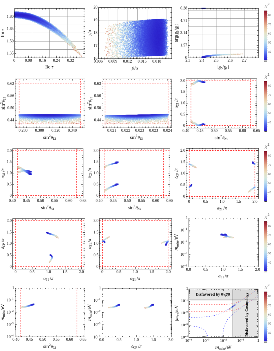
Figure 1: The predictions for the correlations among the input free parameters, neutrino mixing angles, CP violation phases and neutrino masses in the model $\mathcal{B}_{9}$ with NO. The $3\sigma$ bounds of the mixing angles are shown by vertical red dashed lines [47]. Since $\delta_{CP}$ is less constrained, we allow the regions to be in the range $0\sim 2\pi$, and similarly for $\alpha_{21}$ and $\alpha_{31}$. The last panel of $|m_{ee}|$ versus $m_{\text{min}}$ indicates large tightly constrained values for both these neutrino mass observables.

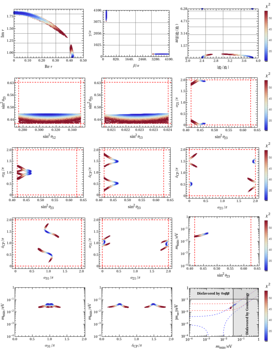
Figure 2: The predictions for the correlations among the input free parameters, neutrino mixing angles, CP violation phases and neutrino masses in the model $\mathcal{B}_{10}$ with NO. Here we adopt the same conventions as figure 1.

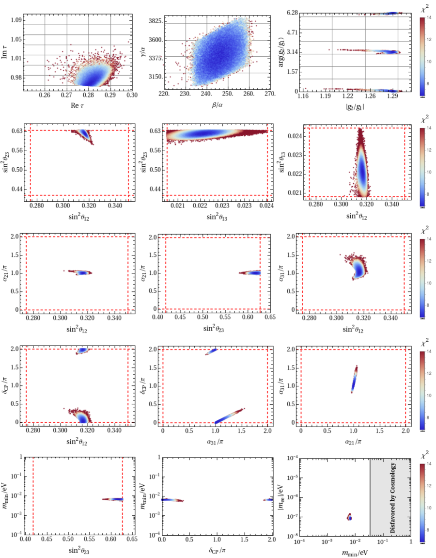
Figure 3: The predictions for the correlations among the input free parameters, neutrino mixing angles, CP violation phases and neutrino masses in the model $\mathcal{D}_{5}$ with NO. Here we adopt the same conventions as figure 1.

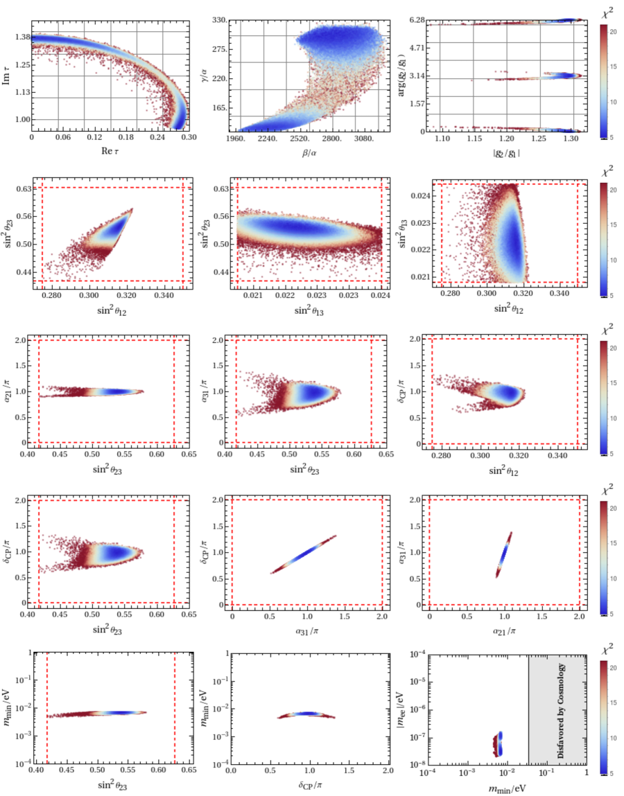
Figure 4: The predictions for the correlations among the input free parameters, neutrino mixing angles, CP violation phases and neutrino masses in the model $\mathcal{D}_{6}$ with NO. Here we adopt the same conventions as figure 1.

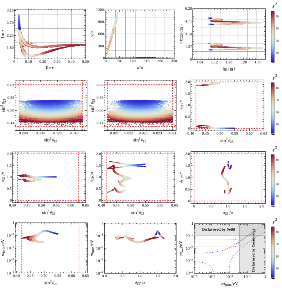
Figure 5: The predictions for the correlations among the input free parameters, neutrino mixing angles, CP violation phases and neutrino masses in the model $\mathcal{D}_{7}$ with NO. Here we adopt the same conventions as figure 1.

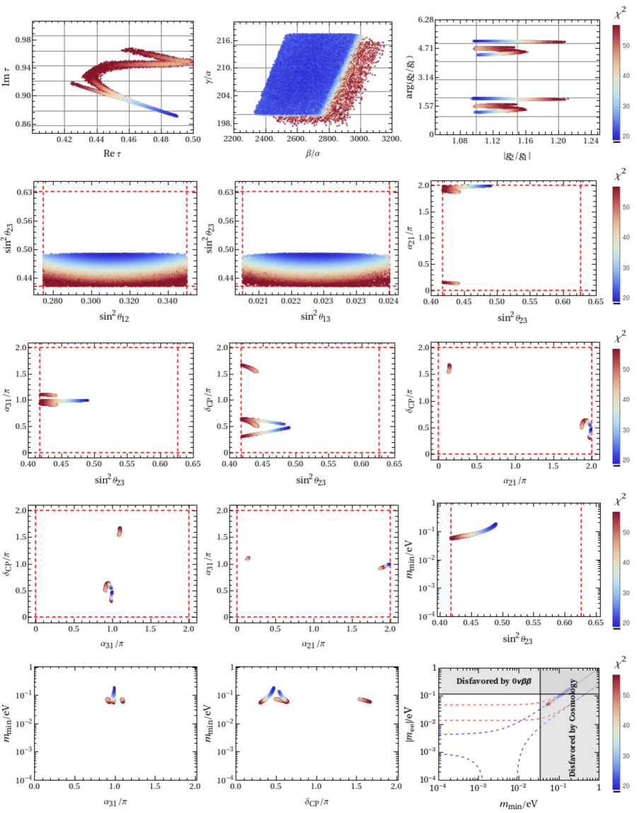
Figure 6: The predictions for the correlations among the input free parameters neutrino mixing angles, CP violation phases and neutrino masses in the model $\mathcal{D}_{8}$ with NO. Here we adopt the same conventions as figure 1.

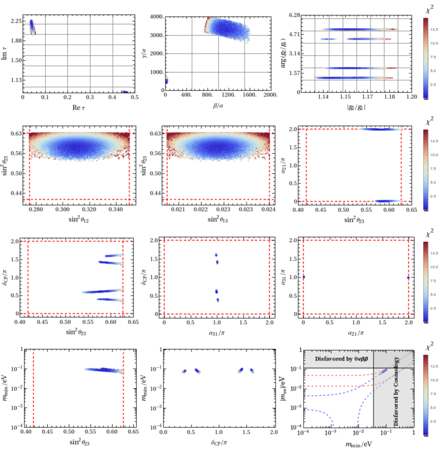
Figure 7: The predictions for the correlations among the input free parameters neutrino mixing angles, CP violation phases and neutrino masses in the model $\mathcal{D}_{9}$ with NO. Here we adopt the same conventions as figure 1.

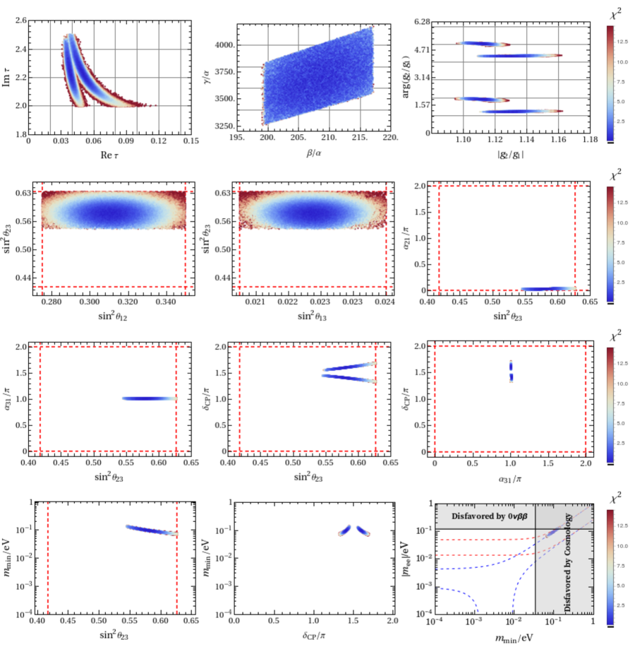
Figure 8: The predictions for the correlations among the input free parameters, neutrino mixing angles, CP violation phases and neutrino masses in the model $\mathcal{D}_{10}$ with NO. Here we adopt the same conventions as figure 1.

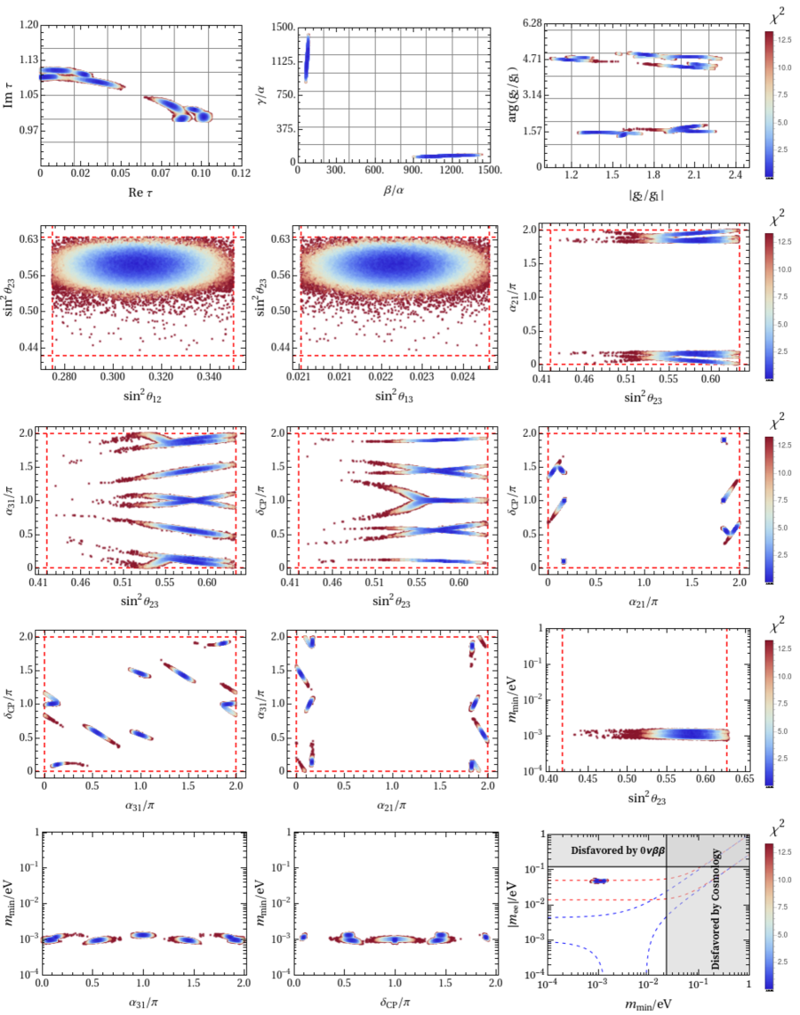
Figure 9: The predictions for the correlations among the input free parameters, neutrino mixing angles, CP violation phases and neutrino masses in the model $\mathcal{B}_{10}$ with IO. Here we adopt the same conventions as figure 1.

The results of the numerical analysis are summarized in tables 6-10. In particular we highlight the new cases $\mathcal{D}_{7}$ and $\mathcal{D}_{9}$ which have a very small $\chi^{2}$ and predict $\delta_{CP}/\pi\approx 1.42-1.45$. We display some interesting correlations of the parameters and observables in these models in figures 1-9, where the colour of the points in these figures indicates the corresponding $\chi^{2}$ value. Note that many of these figures show very tightly constrained regions of observable parameters. For models $\mathcal{B}_{1,2,3}$ and $\mathcal{D}_{1,2,3}$ with two more parameters (which can be see from table 4), we only report the predictions for the observables at the best-fit point, with the results summarized in table 11. The allowed regions of the input parameters and observables are determined by requiring all the lepton mixing angles and the squared mass splittings $\Delta m^{2}_{21}$ and $\Delta m^{2}_{31}$ ($\Delta m^{2}_{32}$) within the $3\sigma$ intervals [47].

Most of these models $\mathcal{B}_{9}$, $\mathcal{B}_{10}$, $\mathcal{D}_{5}\sim\mathcal{D}_{10}$ (apart from $\mathcal{D}_{5}$ and $\mathcal{D}_{6}$) predict large (but allowed) neutrino masses and observable neutrinoless double beta decay. The latest Planck result on the neutrino mass sum is $\sum_{i}m_{i}<0.12~{}\mathrm{eV}-0.60~{}\mathrm{eV}$ [52]. Since the upper bound of the neutrino mass sum sensitively depends on the cosmological model and the choice of other experimental data, we display the full range $0.12~{}\mathrm{eV}-0.60~{}\mathrm{eV}$ as “disfavoured by cosmology” in the figures. Our predictions for neutrino masses could also be probed in next generation neutrinoless double beta decay experiments which is the only feasible experiment having the potential of establishing Majorana nature of neutrinos. The measurement of neutrinoless double beta decay could provide unique information on the neutrino mass spectrum, Majorana phases and the absolute scale of neutrino masses. The decay amplitude is proportional to the effective Majorana mass $m_{ee}$ with the absolute value [53],

$$|m_{ee}|=\left|m_{1}c^{2}_{12}c^{2}_{13}+m_{2}s^{2}_{12}c^{2}_{13}e^{i\alpha_{21}}+m_{3}s^{2}_{13}e^{i(\alpha_{31}-2\delta_{CP})}\right|\,.$$ (59)

The neutrinoless double beta decay experiments can provide valuable information on the neutrino mass spectrum and constrain the Majorana phases. Most of the above models predict neutrino masses in the “cosmologically disfavoured region” and observable neutrinoless double beta decay, which can be tested in forthcoming experiments, with the exception of $\mathcal{D}_{5}$ and $\mathcal{D}_{6}$ which however predict tiny neutrinoless double beta decay, deep into the NO “hole”, together with small Dirac CP violation.

	Model $\mathcal{B}_{9}$		Model $\mathcal{B}_{10}$
	NO		NO
	Best-fit	Allowed regions	Best-fit	Allowed regions
$\Re\langle\tau\rangle$	0.0003	$[0,0.368]$	0.0129	$[0,0.431]$
$\Im\langle\tau\rangle$	1.824	$[1.351,1.856]$	1.824	$[0.91,1.16]\cup[1.31,1.86]$
$\beta/\alpha$	0.018	$[0.008,0.020]$	205.720	$[192.39,215]\cup[3054.254093.49]$
$\gamma/\alpha$	17.560	$[16.046,19.063]$	3612.07	$[192.4,215]\cup[3066.47,4092.98]$
$|g_{2}/g_{1}|$	2.410	$[2.399,2.701]$	2.410	$[2.398,2.71]\cup[2.95,3.86]$
$\arg{(g_{2}/g_{1})}$	0.030	$[0,0.47]\cup[6.25,2\pi]$	6.267	$[0,0.49]\cup[6.23,2\pi]$
$\alpha v_{d}$/MeV	106.523	—	0.5179	—
$(g^{2}_{1}v_{u}^{2}/\Lambda)$/eV	0.011	—	0.0111	—
$m_{e}/m_{\mu}$	0.0048	$[0.0046,0.0050]$	0.0048	$[0.0046,0.0050]$
$m_{\mu}/m_{\tau}$	0.0564	$[0.0520,0.0610]$	0.0564	$[0.0520,0.0610]$
$\sin^{2}\theta_{12}$	0.3096	$[0.2750,0.3500]$	0.3096	$[0.2750,0.3500]$
$\sin^{2}\theta_{13}$	0.02263	$[0.02046,0.02439]$	0.0226	$[0.02045,0.02439]$
$\sin^{2}\theta_{23}$	0.4637	$[0.4180,0.4674]$	0.4638	$[0.4180,0.4676]$
$\delta_{CP}/\pi$	0.510	$[0.17,0.51]\cup[1.24,1.5]$	1.486	$[0.19,0.77]\cup[1.23,1.84]$
$\alpha_{21}/\pi$	0.068	$[0,0.23]\cup[1.78,2]$	0.068	$[0,0.23]\cup[1.77,2]$
$\alpha_{31}/\pi$	1.056	$[0.937,1.270]$	0.948	$[0.683,1.311]$
$m_{1}$/eV	0.0430	$[0.0228,0.0476]$	0.0430	$[0.0225,0.0478]$
$m_{2}$/eV	0.0438	$[0.0244,0.0484]$	0.0439	$[0.0241,0.0485]$
$m_{3}$/eV	0.0661	$[0.0525,0.0716]$	0.0661	$[0.0524,0.0716]$
$\sum_{i}m_{i}$/eV	0.1529	$[0.0997,0.1676]$	0.1530	$[0.0991,0.1679]$
$|m_{ee}|$/eV	0.0435	$[0.0206,0.0483]$	$0.0436$	$[0.0202,0.0483]$
$\chi^{2}_{\mathrm{min}}$	30.77	—	30.72	—

Table 6: The predictions for the best-fit values and the allowed ranges of the input parameters and observables in the models $\mathcal{B}_{9}$ and $\mathcal{B}_{10}$ with NO. We would like to emphasize that the Dirac CP phase $\delta_{CP}\simeq 1.49\pi$ at the conjugate best fit point $\tau\rightarrow-\tau^{*},g_{i}\rightarrow g^{*}_{i}$ in model $\mathcal{B}_{9}$.

	Model $\mathcal{D}_{5}$		Model $\mathcal{D}_{6}$
	NO		NO
	Best-fit	Allowed regions	Best-fit	Allowed regions
$\Re\langle\tau\rangle$	0.280	$[0.248,0.300]$	0.279	$[0.0,0.300]$
$\Im\langle\tau\rangle$	0.960	$[0.957,1.056]$	0.960	$[0.957,1.394]$
$\beta/\alpha$	244.708	$[216.359,266.608]$	2774.426	$[1954.8,3290.0]$
$\gamma/\alpha$	3397.7	$[2991.9,3880.4]$	302.315	$[118.236,327.297]$
$|g_{2}/g_{1}|$	1.293	$[1.143,1.308]$	1.294	$[1.034,1.314]$
$\arg{(g_{2}/g_{1})}$	0	$[0,0.23]\cup[3.01,3.37]$	3.142	$[0.0,0.29]\cup[2.85,3.38]$
		$\cup[6.1,2\pi]$		$\cup[5.97,2\pi]$
$\alpha v_{d}$/MeV	0.4174	—	0.4177	—
$(g^{2}_{1}v_{u}^{2}/\Lambda)$/eV	0.01321	—	0.01321	—
$m_{e}/m_{\mu}$	0.0048	$[0.0046,0.0050]$	0.0048	$[0.0046,0.0050]$
$m_{\mu}/m_{\tau}$	0.0569	$[0.0520,0.0610]$	0.0561	$[0.0520,0.0610]$
$\sin^{2}\theta_{12}$	0.3169	$[0.3011,0.3244]$	0.3161	$[0.2752,0.3241]$
$\sin^{2}\theta_{13}$	0.02189	$[0.02045,0.02439]$	0.0220	$[0.02045,0.02439]$
$\sin^{2}\theta_{23}$	0.6171	$[0.5754,0.627]$	0.5396	$[0.4186,0.5845]$
$\delta_{CP}/\pi$	0	$[0,0.41]\cup[1.79,2]$	$1.0$	$[0.57,1.33]$
$\alpha_{21}/\pi$	1.0	$[0.959,1.071]$	1.0	$[0.89,1.1]$
$\alpha_{31}/\pi$	1.0	$[0.746,1.603]$	1.0	$[0.495,1.396]$
$m_{1}$/eV	0.0067	$[0.0052,0.0069]$	0.0067	$[0.0042,0.0069]$
$m_{2}$/eV	0.0109	$[0.0100,0.0110]$	0.0109	$[0.0095,0.0110]$
$m_{3}$/eV	0.0499	$[0.0476,0.0520]$	0.0501	$[0.0476,0.0539]$
$\sum_{i}m_{i}$/eV	0.0675	$[0.0628,0.0699]$	0.0677	$[0.0613,0.0717]$
$|m_{ee}|$/eV	$10^{-8}$	$[10^{-8},10^{-7}]$	$10^{-7}$	$[10^{-8},10^{-7}]$
$\chi^{2}_{\mathrm{min}}$	6.82	—	4.857	—

Table 7: The predictions for the best-fit values and the allowed ranges of the input parameters and observables in the models $\mathcal{D}_{5}$ and $\mathcal{D}_{6}$ with NO.

	Model $\mathcal{D}_{7}$		Model $\mathcal{D}_{8}$
	NO		NO
	Best-fit	Allowed regions	Best-fit	Allowed regions
$\Re\langle\tau\rangle$	0.0428	$[0.026,0.5]$	0.471	$[0.424,0.5]$
$\Im\langle\tau\rangle$	2.105	$[1.468,3.006]$	0.886	$[0.872,0.964]$
$\beta/\alpha$	0.473	$[0.048,339.73]$	2646.6	$[2327.7,3181.7]$
$\gamma/\alpha$	0.002	$[0.002,1140.03]$	208.094	$[197.1,217.356]$
$|g_{2}/g_{1}|$	1.154	$[1.084,1.385]$	1.113	$[1.094,1.212]$
$\arg{(g_{2}/g_{1})}$	1.964	$[1.16,1.98]\cup[4.3,5.12]$	1.227	$[1.19,1.98]\cup[4.34,5.12]$
$\alpha v_{d}$/MeV	1702.3	—	0.368	—
$(g^{2}_{1}v_{u}^{2}/\Lambda)$/eV	0.0405	—	0.036	—
$m_{e}/m_{\mu}$	0.0048	$[0.0046,0.0050]$	0.0048	$[0.0046,0.0050]$
$m_{\mu}/m_{\tau}$	0.0565	$[0.0520,0.0610]$	0.0565	$[0.0520,0.0610]$
$\sin^{2}\theta_{12}$	0.3100	$[0.2750,0.3500]$	0.3105	$[0.2750,0.3500]$
$\sin^{2}\theta_{13}$	0.0224	$[0.02045,0.02439]$	0.0224	$[0.02045,0.02439]$
$\sin^{2}\theta_{23}$	0.580	$[0.418,0.551]$	0.4698	$[0.418,0.491]$
$\delta_{CP}/\pi$	1.60	$[0.307,1.702]$	$1.522$	$[0.29,0.65]\cup[1.52,1.68]$
$\alpha_{21}/\pi$	1.99	$[0,0.14]\cup[1.84,2]$	0	$[0.12,0.16]\cup[1.86,2]$
$\alpha_{31}/\pi$	0.986	$[0.806,1.1]$	1.002	$[0.898,1.115]$
$m_{1}$/eV	0.0805	$[0.0250,0.2437]$	0.1003	$[0.0505,0.1885]$
$m_{2}$/eV	0.0810	$[0.0264,0.2438]$	0.1007	$[0.0512,0.1887]$
$m_{3}$/eV	0.0949	$[0.0537,0.2495]$	0.1122	$[0.0695,0.1956]$
$\sum_{i}m_{i}$/eV	0.2564	$[0.1051,0.7370]$	0.3132	$[0.1712,0.5729]$
$|m_{ee}|$/eV	0.0805	$[0.0235,0.2438]$	0.1004	$[0.0501,0.1887]$
$\chi^{2}_{\mathrm{min}}$	0.0003	—	27.5	—

Table 8: The predictions for the best-fit values and the allowed ranges of the input parameters and observables in the models $\mathcal{D}_{7}$ and $\mathcal{D}_{8}$ with NO.

	Model $\mathcal{D}_{9}$		Model $\mathcal{D}_{10}$
	NO		NO
	Best-fit	Allowed regions	Best-fit	Allowed regions
$\Re\langle\tau\rangle$	0.0387	$[0.033,0.056]\cup[0.44,0.469]$	0.0386	$[0.0307,0.1175]$
$\Im\langle\tau\rangle$	2.233	$[0.887,0.908]\cup[2.0,2.282]$	2.230	$[1.996,2.50]$
$\beta/\alpha$	23.195	$[21.24,38.95]\cup[737.8,1599.9]$	207.908	$[198.963,217.263]$
$\gamma/\alpha$	410.532	$[352.32,700]\cup[2520.65,3983.95]$	3673.38	$[3254.84,4170.84]$
$|g_{2}/g_{1}|$	1.138	$[1.127,1.190]$	1.129	$[1.094,1.162]$
$\arg{(g_{2}/g_{1})}$	1.172	$[1.16,1.21]\cup[1.93,1.98]$	1.197	$[1.17,1.25]\cup[1.76,1.95]$
		$\cup[4.3,4.35]\cup[5.07,5.13]$		$\cup[4.31,4.4]\cup[4.9,5.09]$
$\alpha v_{d}$/MeV	4.585	—	0.512	—
$(g^{2}_{1}v_{u}^{2}/\Lambda)$/eV	0.0476	—	0.0475	—
$m_{e}/m_{\mu}$	0.0048	$[0.0046,0.0050]$	0.0048	$[0.0046,0.0050]$
$m_{\mu}/m_{\tau}$	0.0565	$[0.0520,0.0610]$	0.0565	$[0.0520,0.0610]$
$\sin^{2}\theta_{12}$	0.3098	$[0.2750,0.3500]$	0.3098	$[0.2750,0.3500]$
$\sin^{2}\theta_{13}$	0.0224	$[0.02045,0.02439]$	0.0224	$[0.02045,0.02439]$
$\sin^{2}\theta_{23}$	0.5807	$[0.5353,0.6270]$	0.580	$[0.5456,0.6270]$
$\delta_{CP}/\pi$	1.420	$[0.35,0.4]\cup[0.58,0.66]$	1.604	$[1.33,1.45]\cup[1.55,1.7]$
		$\cup[1.36,1.43]\cup[1.58,1.63]$
$\alpha_{21}/\pi$	0.006	$[0,0.01]\cup[1.98,2]$	0.015	$[0.009,0.0373]$
$\alpha_{31}/\pi$	1.005	$[0.978,1.027]$	1.007	$[1.003,1.029]$
$m_{1}$/eV	0.0948	$[0.0601,0.1044]$	0.0946	$[0.0658,0.1378]$
$m_{2}$/eV	0.0952	$[0.0607,0.1048]$	0.0950	$[0.0663,0.1381]$
$m_{3}$/eV	0.1073	$[0.0765,0.1167]$	0.1071	$[0.0811,0.1476]$
$\sum_{i}m_{i}$/eV	0.2974	$[0.1973,0.3259]$	0.2966	$[0.2132,0.4234]$
$|m_{ee}|$/eV	0.0949	$[0.0599,0.1045]$	0.0945	$[0.0651,0.1379]$
$\chi^{2}_{\mathrm{min}}$	0.0023	—	0.0003	—

Table 9: The predictions for the the best-fit values and the allowed ranges of the input parameters and observables in the model $\mathcal{D}_{9}$ and $\mathcal{D}_{10}$ with NO.

Model $\mathcal{B}_{10}$	IO
	Best-fit	Allowed regions
$\Re\langle\tau\rangle$	0.096	$[0,0.102]$
$\Im\langle\tau\rangle$	0.987	$[0.98,1.049]\cup[1.052,1.109]$
$\beta/\alpha$	79.472	$[59.68,86.37]\cup[892.67,1446.02]$
$\gamma/\alpha$	1232.57	$[60.97,86.34]\cup[870.16,1443.84]$
$|g_{2}/g_{1}|$	2.093	$[1.038,2.453]$
$\arg{(g_{2}/g_{1})}$	4.715	$[1.33,1.83]\cup[4.29,5]$
$\alpha v_{d}$/MeV	1.167	—
$(g^{2}_{1}v_{u}^{2}/\Lambda)$/eV	0.004	—
$m_{e}/m_{\mu}$	0.0048	$[0.0046,0.0050]$
$m_{\mu}/m_{\tau}$	0.0565	$[0.0520,0.0610]$
$\sin^{2}\theta_{12}$	0.3100	$[0.2750,0.3500]$
$\sin^{2}\theta_{13}$	0.02264	$[0.02068,0.02463]$
$\sin^{2}\theta_{23}$	0.584	$[0.423,0.629]$
$\delta_{CP}/\pi$	1.458	$[0.068,1.933]$
$\alpha_{21}/\pi$	0.138	$[0,0.19]\cup[1.8,2]$
$\alpha_{31}/\pi$	0.997	$[0,2]$
$m_{1}$/eV	0.0494	$[0.0464,0.0526]$
$m_{2}$/eV	0.0501	$[0.0472,0.0533]$
$m_{3}$/eV	0.0013	$[0.0007,0.0015]$
$\sum_{i}m_{i}$/eV	0.1008	$[0.0942,0.1074]$
$|m_{ee}|$/eV	0.0475	$[0.0439,0.0516]$
$\chi^{2}_{\mathrm{min}}$	$10^{-7}$	—

Table 10: The predictions for the best-fit values and the allowed ranges of the input parameters and observables in the model $\mathcal{B}_{10}$ with IO.

Models	$\mathcal{B}_{1}$	$\mathcal{B}_{2}$	$\mathcal{B}_{3}$	$\mathcal{D}_{1}$	$\mathcal{D}_{2}$	$\mathcal{D}_{3}$
	Best-fit values for NO
$\Re\langle\tau\rangle$	0.485	0.468	0.487	0.101	0.099	0.109
$\Im\langle\tau\rangle$	1.150	1.222	1.574	1.250	1.428	1.359
$\beta/\alpha$	632.056	2610.95	288.448	111.715	143.544	253.671
$\gamma_{1}/\alpha$	59.950	218.726	1177.58	1306.5	1109.25	21.804
$|\gamma_{2}/\alpha|$	9.452	211.488	1201.62	796.746	801.233	3.549
$\arg{(\gamma_{2}/\alpha)}$	2.871	3.046	3.523	4.055	2.487	4.421
$|g_{2}/g_{1}|$	0.992	1.122	1.647	1.109	1.543	1.264
$\arg{(g_{2}/g_{1})}$	2.203	2.398	2.081	6.024	0.889	0.014
$\alpha v_{d}$/MeV	2.374	0.613	1.499	1.201	1.597	6.965
$(g^{2}_{1}v_{u}^{2}/\Lambda)$/eV	0.0109	0.0103	0.0114	0.0155	0.0122	0.0173
$m_{e}/m_{\mu}$	0.0048	0.0048	0.0048	0.0048	0.0048	0.0048
$m_{\mu}/m_{\tau}$	0.0565	0.0565	0.0565	0.0565	0.0565	0.0565
$\sin^{2}\theta_{12}$	0.3100	0.3100	0.3100	0.3100	0.3100	0.3100
$\sin^{2}\theta_{13}$	0.02241	0.02241	0.02241	0.02241	0.02241	0.02241
$\sin^{2}\theta_{23}$	0.5800	0.5800	0.5800	0.5800	0.5800	0.5800
$\delta_{CP}/\pi$	0.556	1.391	1.20	1.586	0.320	0.893
$\alpha_{21}/\pi$	0.811	1.015	0.997	1.623	1.363	0.927
$\alpha_{31}/\pi$	0.403	1.071	0.154	1.167	0.118	1.042
$m_{1}$/eV	0.0204	0.0162	0.0335	0.0048	0.0212	0.0063
$m_{2}$/eV	0.0222	0.0183	0.0346	0.0098	0.0229	0.0107
$m_{3}$/eV	0.0542	0.0528	0.0604	0.0505	0.0545	0.0506
$\sum_{i}m_{i}$/eV	0.0969	0.0872	0.1285	0.0651	0.0987	0.0677
$|m_{ee}|$/eV	0.0080	0.0061	0.0131	0.0061	0.0136	0.00036
$\chi^{2}_{\mathrm{min}}$	$10^{-6}$	$10^{-6}$	$10^{-6}$	$10^{-7}$	$10^{-7}$	$10^{-6}$

Table 11: The predictions for the best-fit values of the input parameters and observables in the models $\mathcal{B}_{1,2,3}$ and $\mathcal{D}_{1,2,3}$ with NO ordering.

5 Conclusion

In this paper we have provided a comprehensive analysis of lepton masses and mixing in theories with $\Gamma_{3}\cong A_{4}$ modular symmetry, where the single modulus field $\tau$ is the unique source of flavour symmetry breaking, with no flavons allowed, and all masses and Yukawa couplings are modular forms. Similar to previous analyses, we have discussed all the simplest neutrino sectors arising from both the Weinberg operator and the type I seesaw mechanism, with lepton doublets and right-handed neutrinos assumed to be triplets of $A_{4}$. Unlike previous analyses, we have allowed right-handed charged leptons to transform as all combinations of $\mathbf{1}$, $\mathbf{1}^{\prime}$ and $\mathbf{1}^{\prime\prime}$ representations of $A_{4}$, using the simplest different modular weights to break the degeneracy, leading to ten different charged lepton Yukawa matrices, instead of the usual one.

The above considerations imply ten different Weinberg models, labelled as $\mathcal{A}_{1}$-$\mathcal{A}_{10}$, and thirty different type I seesaw models, labelled as $\mathcal{B}_{1}$-$\mathcal{B}_{10}$, $\mathcal{C}_{1}$-$\mathcal{C}_{10}$, $\mathcal{D}_{1}$-$\mathcal{D}_{10}$, which we have analyzed in detail, in the form of extensive sets of figures and tables. The results of the numerical analysis are summarised in table 5, where we see that fourteen models for both NO and IO can accommodate the data, indicated by “✔”, where the original model corresponds to the case of $\mathcal{D}_{10}$ and all the other successful models are new. Interestingly, most of the successful patterns $\mathcal{B}_{9},\,\mathcal{B}_{10},\,\mathcal{D}_{5}\sim\mathcal{D}_{10}$ (apart from $\mathcal{D}_{5}\sim\mathcal{D}_{6}$) predict tightly constrained values for the mixing parameters and large neutrino mass observables $|m_{ee}|$ and $m_{\text{min}}$, together with approximately maximal Dirac phase. There are also other interesting correlations among the mixing parameters for these models.

The most successful models $\mathcal{B}_{9}$, $\mathcal{B}_{10}$, $\mathcal{D}_{5}\sim\mathcal{D}_{10}$ all contain six real free parameters and two overall mass scales, describing the entire lepton sector (three charged lepton masses, three neutrino masses, three lepton mixing angles and three CP violating phases). These are the minimal models of $\Gamma_{3}$ modular-invariant supersymmetry theories allowed by experiment. The results presented here provide new opportunities for $A_{4}$ modular symmetry model building, including possible extensions to the quark sector.

Acknowledgements

G.-J.  D. and X.-G.  L. acknowledges the support of the National Natural Science Foundation of China under Grant Nos 11522546 and 11835013. S. F. K. acknowledges the STFC Consolidated Grant ST/L000296/1 and the European Union’s Horizon 2020 research and innovation programme under the Marie Skłodowska-Curie grant agreements Elusives ITN No. 674896 and InvisiblesPlus RISE No. 690575. G.-J.  D. and X.-G.  L. are grateful to Dr. Yang Zhang for his kind help on the MultiNest program.

References

- [1] S. F. King and C. Luhn, “Neutrino Mass and Mixing with Discrete Symmetry,” Rept. Prog. Phys. 76 (2013) 056201, arXiv:1301.1340 [hep-ph].
- [2] S. F. King, “Unified Models of Neutrinos, Flavour and CP Violation,” Prog. Part. Nucl. Phys. 94 (2017) 217–256, arXiv:1701.04413 [hep-ph].
- [3] Y. Koide, “S(4) flavor symmetry embedded into SU(3) and lepton masses and mixing,” JHEP 08 (2007) 086, arXiv:0705.2275 [hep-ph].
- [4] T. Banks and N. Seiberg, “Symmetries and Strings in Field Theory and Gravity,” Phys. Rev. D83 (2011) 084019, arXiv:1011.5120 [hep-th].
- [5] Y.-L. Wu, “SU(3) Gauge Family Symmetry and Prediction for the Lepton-Flavor Mixing and Neutrino Masses with Maximal Spontaneous CP Violation,” Phys. Lett. B714 (2012) 286–294, arXiv:1203.2382 [hep-ph].
- [6] A. Merle and R. Zwicky, “Explicit and spontaneous breaking of SU(3) into its finite subgroups,” JHEP 02 (2012) 128, arXiv:1110.4891 [hep-ph].
- [7] B. L. Rachlin and T. W. Kephart, “Spontaneous Breaking of Gauge Groups to Discrete Symmetries,” JHEP 08 (2017) 110, arXiv:1702.08073 [hep-ph].
- [8] C. Luhn, “Spontaneous breaking of SU(3) to finite family symmetries: a pedestrian’s approach,” JHEP 03 (2011) 108, arXiv:1101.2417 [hep-ph].
- [9] S. F. King and Y.-L. Zhou, “Spontaneous breaking of to finite family symmetries with supersymmetry - an model,” JHEP 11 (2018) 173, arXiv:1809.10292 [hep-ph].
- [10] G. Altarelli, F. Feruglio, and C. Hagedorn, “A SUSY SU(5) Grand Unified Model of Tri-Bimaximal Mixing from A4,” JHEP 03 (2008) 052, arXiv:0802.0090 [hep-ph].
- [11] T. J. Burrows and S. F. King, “A(4) Family Symmetry from SU(5) SUSY GUTs in 6d,” Nucl. Phys. B835 (2010) 174–196, arXiv:0909.1433 [hep-ph].
- [12] T. J. Burrows and S. F. King, “ x SU(5) SUSY GUT of Flavour in 8d,” Nucl. Phys. B842 (2011) 107–121, arXiv:1007.2310 [hep-ph].
- [13] F. J. de Anda and S. F. King, “An SUSY GUT of flavour in 6d,” JHEP 07 (2018) 057, arXiv:1803.04978 [hep-ph].
- [14] A. Adulpravitchai, A. Blum, and M. Lindner, “Non-Abelian Discrete Flavor Symmetries from T**2/Z(N) Orbifolds,” JHEP 07 (2009) 053, arXiv:0906.0468 [hep-ph].
- [15] T. Asaka, W. Buchmuller, and L. Covi, “Gauge unification in six-dimensions,” Phys. Lett. B523 (2001) 199–204, arXiv:hep-ph/0108021 [hep-ph].
- [16] G. Altarelli, F. Feruglio, and Y. Lin, “Tri-bimaximal neutrino mixing from orbifolding,” Nucl. Phys. B775 (2007) 31–44, arXiv:hep-ph/0610165 [hep-ph].
- [17] A. Adulpravitchai and M. A. Schmidt, “Flavored Orbifold GUT - an SO(10) x S4 model,” JHEP 01 (2011) 106, arXiv:1001.3172 [hep-ph].
- [18] T. Kobayashi, H. P. Nilles, F. Ploger, S. Raby, and M. Ratz, “Stringy origin of non-Abelian discrete flavor symmetries,” Nucl. Phys. B768 (2007) 135–156, arXiv:hep-ph/0611020 [hep-ph].
- [19] F. J. de Anda and S. F. King, “ in 6d,” JHEP 10 (2018) 128, arXiv:1807.07078 [hep-ph].
- [20] T. Kobayashi, S. Nagamoto, S. Takada, S. Tamba, and T. H. Tatsuishi, “Modular symmetry and non-Abelian discrete flavor symmetries in string compactification,” Phys. Rev. D97 no. 11, (2018) 116002, arXiv:1804.06644 [hep-th].
- [21] A. Baur, H. P. Nilles, A. Trautner, and P. K. S. Vaudrevange, “Unification of Flavor, CP, and Modular Symmetries,” arXiv:1901.03251 [hep-th].
- [22] A. Giveon, E. Rabinovici, and G. Veneziano, “Duality in String Background Space,” Nucl. Phys. B322 (1989) 167–184.
- [23] G. Altarelli and F. Feruglio, “Tri-bimaximal neutrino mixing, A(4) and the modular symmetry,” Nucl. Phys. B741 (2006) 215–235, arXiv:hep-ph/0512103 [hep-ph].
- [24] R. de Adelhart Toorop, F. Feruglio, and C. Hagedorn, “Finite Modular Groups and Lepton Mixing,” Nucl. Phys. B858 (2012) 437–467, arXiv:1112.1340 [hep-ph].
- [25] F. Feruglio, “Are neutrino masses modular forms?,” in From My Vast Repertoire …: Guido Altarelli’s Legacy, A. Levy, S. Forte, and G. Ridolfi, eds., pp. 227–266. 2019. arXiv:1706.08749 [hep-ph].
- [26] J. C. Criado and F. Feruglio, “Modular Invariance Faces Precision Neutrino Data,” arXiv:1807.01125 [hep-ph].
- [27] T. Kobayashi, K. Tanaka, and T. H. Tatsuishi, “Neutrino mixing from finite modular groups,” Phys. Rev. D98 no. 1, (2018) 016004, arXiv:1803.10391 [hep-ph].
- [28] T. Kobayashi, Y. Shimizu, K. Takagi, M. Tanimoto, T. H. Tatsuishi, and H. Uchida, “Finite modular subgroups for fermion mass matrices and baryon/lepton number violation,” arXiv:1812.11072 [hep-ph].
- [29] T. Kobayashi, Y. Shimizu, K. Takagi, M. Tanimoto, and T. H. Tatsuishi, “Modular invariant flavor model in SU(5) GUT,” arXiv:1906.10341 [hep-ph].
- [30] H. Okada and Y. Orikasa, “A modular symmetric radiative seesaw model,” arXiv:1907.04716 [hep-ph].
- [31] T. Kobayashi, N. Omoto, Y. Shimizu, K. Takagi, M. Tanimoto, and T. H. Tatsuishi, “Modular invariance and neutrino mixing,” arXiv:1808.03012 [hep-ph].
- [32] H. Okada and M. Tanimoto, “CP violation of quarks in modular invariance,” arXiv:1812.09677 [hep-ph].
- [33] P. P. Novichkov, S. T. Petcov, and M. Tanimoto, “Trimaximal Neutrino Mixing from Modular A4 Invariance with Residual Symmetries,” arXiv:1812.11289 [hep-ph].
- [34] T. Nomura and H. Okada, “A two loop induced neutrino mass model with modular symmetry,” arXiv:1906.03927 [hep-ph].
- [35] J. T. Penedo and S. T. Petcov, “Lepton Masses and Mixing from Modular Symmetry,” Nucl. Phys. B939 (2019) 292–307, arXiv:1806.11040 [hep-ph].
- [36] P. P. Novichkov, J. T. Penedo, S. T. Petcov, and A. V. Titov, “Modular Models of Lepton Masses and Mixing,” arXiv:1811.04933 [hep-ph].
- [37] T. Kobayashi, Y. Shimizu, K. Takagi, M. Tanimoto, and T. H. Tatsuishi, “New lepton flavor model from modular symmetry,” arXiv:1907.09141 [hep-ph].
- [38] P. P. Novichkov, J. T. Penedo, S. T. Petcov, and A. V. Titov, “Modular Symmetry for Flavour Model Building,” arXiv:1812.02158 [hep-ph].
- [39] G.-J. Ding, S. F. King, and X.-G. Liu, “Neutrino Mass and Mixing with Modular Symmetry,” arXiv:1903.12588 [hep-ph].
- [40] F. J. de Anda, S. F. King, and E. Perdomo, “ Grand Unified Theory with Modular Symmetry,” arXiv:1812.05620 [hep-ph].
- [41] I. de Medeiros Varzielas, S. F. King, and Y.-L. Zhou, “Multiple modular symmetries as the origin of flavour,” arXiv:1906.02208 [hep-ph].
- [42] P. P. Novichkov, J. T. Penedo, S. T. Petcov, and A. V. Titov, “Generalised CP Symmetry in Modular-Invariant Models of Flavour,” arXiv:1905.11970 [hep-ph].
- [43] X.-G. Liu and G.-J. Ding, “Neutrino Masses and Mixing from Double Covering of Finite Modular Groups,” arXiv:1907.01488 [hep-ph].
- [44] J. H. Bruinier, G. V. D. Geer, G. Harder, and D. Zagier, The 1-2-3 of Modular Forms. Universitext. Springer Berlin Heidelberg, 2008.
- [45] F. Diamond and J. M. Shurman, A first course in modular forms, vol. 228 of Graduate Texts in Mathematics. Springer, 2005.
- [46] R. C. Gunning, Lectures on Modular Forms. Princeton, New Jersey USA, Princeton University Press, 1962.
- [47] I. Esteban, M. C. Gonzalez-Garcia, A. Hernandez-Cabezudo, M. Maltoni, and T. Schwetz, “Global analysis of three-flavour neutrino oscillations: synergies and tensions in the determination of , and the mass ordering,” arXiv:1811.05487 [hep-ph].
- [48] F. Feruglio, K. M. Patel, and D. Vicino, “Order and Anarchy hand in hand in 5D SO(10),” JHEP 09 (2014) 095, arXiv:1407.2913 [hep-ph].
- [49] G. Ross and M. Serna, “Unification and fermion mass structure,” Phys. Lett. B664 (2008) 97–102, arXiv:0704.1248 [hep-ph].
- [50] F. Feroz and M. P. Hobson, “Multimodal nested sampling: an efficient and robust alternative to MCMC methods for astronomical data analysis,” Mon. Not. Roy. Astron. Soc. 384 (2008) 449, arXiv:0704.3704 [astro-ph].
- [51] F. Feroz, M. P. Hobson, and M. Bridges, “MultiNest: an efficient and robust Bayesian inference tool for cosmology and particle physics,” Mon. Not. Roy. Astron. Soc. 398 (2009) 1601–1614, arXiv:0809.3437 [astro-ph].
- [52] Planck Collaboration, N. Aghanim et al., “Planck 2018 results. VI. Cosmological parameters,” arXiv:1807.06209 [astro-ph.CO].
- [53] Particle Data Group Collaboration, M. Tanabashi et al., “Review of Particle Physics,” Phys. Rev. D98 no. 3, (2018) 030001.