Diffusion Phenomena in a Mixed Phase Space

Abstract

We show that, in strongly chaotic dynamical systems, the average particle velocity can be calculated analytically by consideration of Brownian dynamics in phase space, the method of images and use of the classical diffusion equation. The method is demonstrated on the simplified Fermi-Ulam accelerator model, which has a mixed phase space with chaotic seas, invariant tori and Kolmogorov-Arnold-Moser (KAM) islands. The calculated average velocities agree well with numerical simulations and with an earlier empirical theory. The procedure can readily be extended to other systems including time-dependent billiards.

We present an approach to the analysis of complicated chaotic dynamical systems that are difficult to treat in other ways. It relies on the counter-intuitive application of a fundamental idea from classical continuum physics (probabilistic diffusion) to chaotic systems that are, of course, inherently deterministic. In particular, we consider diffusion and Brownian dynamics in the phase space of the chaotic system and show how the diffusion equation, applied in this unusual context, can provide an accurate description of the average velocity and its evolution. To demonstrate and validate the formalism, we take a well-known example from astrophysics - the Fermi-Ulam model.

I Introduction

The evolution of systems described by Hamiltonians with nonlinear terms in their dynamical equations may exhibit either regularity or chaos. The result is often a mixed phase space containing chaotic seas, invariant tori and Kolmogorov-Arnold-Moser (KAM) islands lich . Dynamical systems with strong chaotic motion often exhibit diffusive behavior ott ; chirikov . An intuitive example of this is to drop colored ink into water, observing how the particles of ink move away from each other, spreading out into the liquid. For a mixed phase space, however, an initial condition e.g. around a KAM island may lead to very complicated behavior. The stability structures influence directly the transport properties of chaotic orbits venegeroles1 , often generating so-called anomalous diffusion zasla ; robnik .

There are many scenarios where, rather than analysing the individual behaviour of a single particle starting from a particular initial condition, it is more interesting to consider the average properties of the system, taking into account an ensemble of particles. Statistical methods can then be used to describe the dynamical phenomena venegeroles2 ; meiss ; manchein . Correspondingly, the properties and construction of the phase space can lead to what are effectively diffusion processes: as the dynamics evolves, there is diffusion of the action, usually associated with the velocity of the particles, through the phase space.

In this work we show that the classical diffusion equation dif1 ; dif2 ; dif3 ; dif4 ; dif5 can be solved via a procedure well-known in electrostatics, namely the method of images, and used to describe the evolution of the average velocity for a system characterised by a mixed phase space. We will demonstrate the effectiveness and utility of this idea by applying it to the well-known and widely-studied Fermi-Ulam model (FUM).

This paper is organised as follows. In Sec. II we describe the FUM, showing the nonlinear map associated with the dynamics and introducing a picture of a diffusion process occurring within its characteristic phase space. Section III develops a theoretical framework yielding analytical results for normal diffusion in a mixed phase space. In Sec. IV we compare these analytical results with numerical data. Conclusions are drawn in Sec. V.

II Model and phase space

The FUM fum is a version of the Fermi accelerator, which was originally introduced by Enrico Fermi fermi as a possible explanation for the production of very high energy cosmic rays. Its acceleration mechanism involves the repulsion of an electrically charged particle by strong oscillatory magnetic fields, a process that is analogous to a classical particle colliding with an oscillating physical boundary. The model consists of a particle bouncing back and forth between two rigid walls, one of which is fixed, whereas the other moves periodically in time with a normalized amplitude $\varepsilon$, as shown schematically in Fig.1.

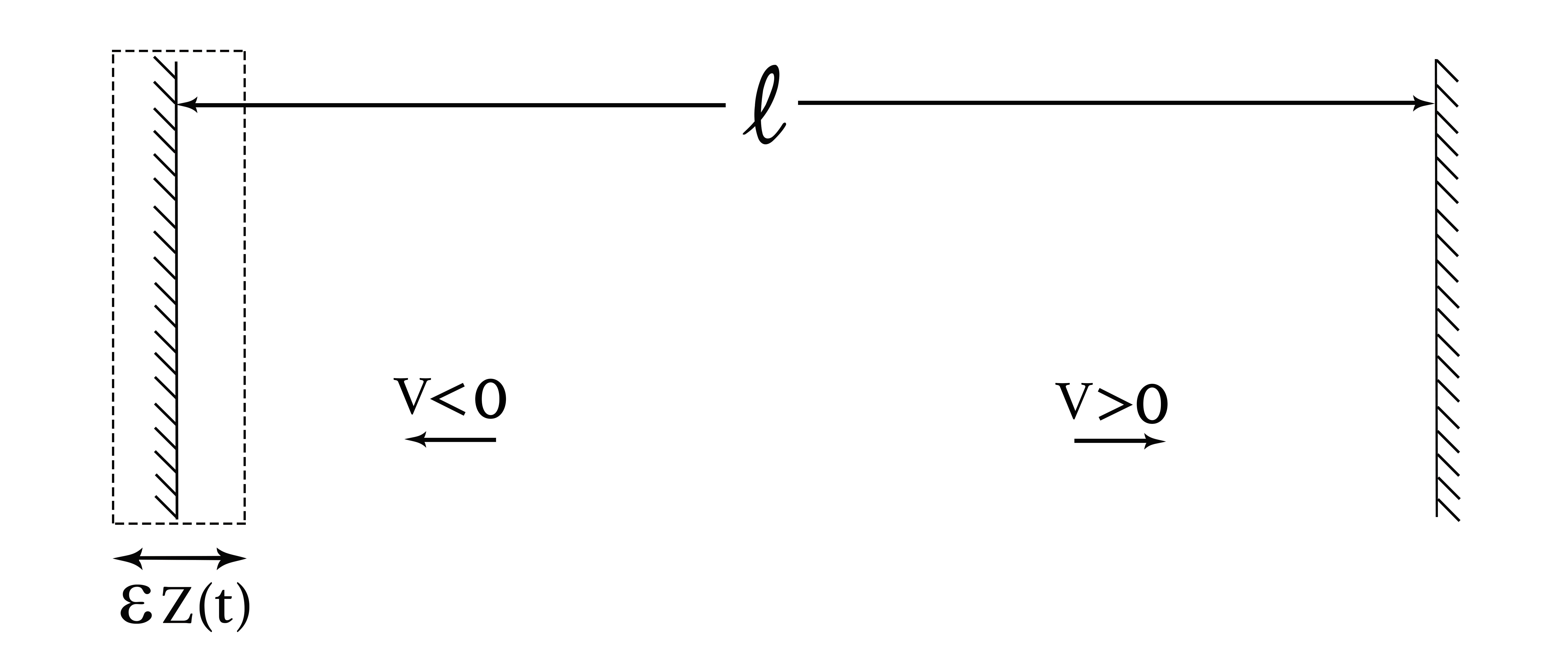
Figure 1: Illustration of the Fermi-Ulam model. The geometrical parameter $\ell$ is the distance between the two walls and the direction of the vectors denotes the sign of the particle’s velocity. Usually the time-dependent function $Z(t)$ is chosen as $\cos(\omega t)$, with $\omega$ the frequency of oscillation.

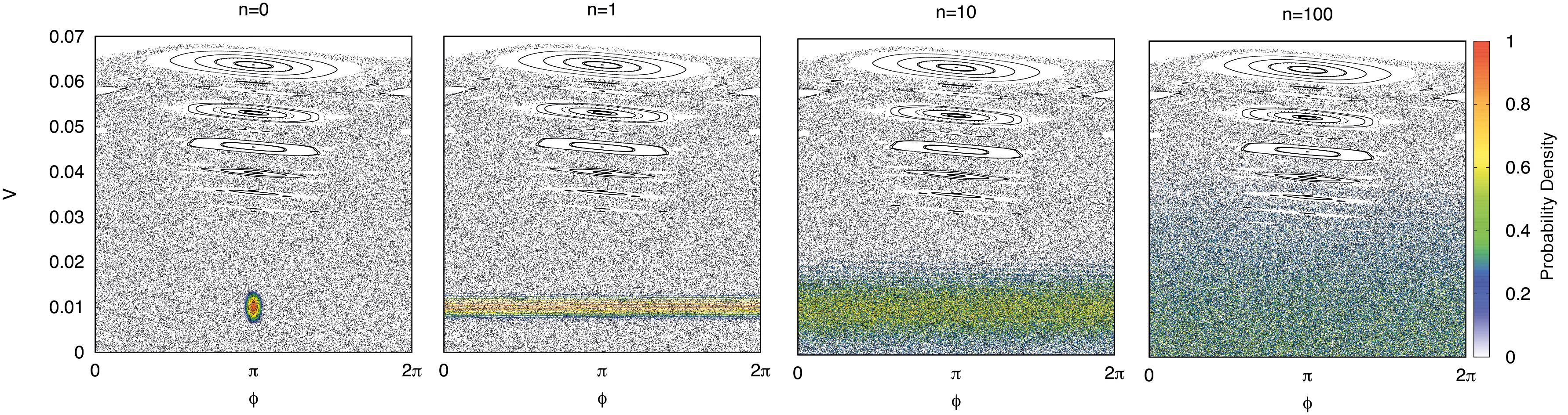
Figure 2: (colour online). Phase space diffusion in the FUM, as sketched in Fig. 1 and described by the mapping (1). It is illustrated by the probability density in a chaotic region of the FUM’s phase space, for different numbers of iterations $n$. The colour scale shows how likely it is to find an orbit at that area of the phase space. The initial distribution, centered at $\phi_{0}=\pi$, $V_{0}=0.01$ with a standard deviation $\sigma_{\phi_{0}}=0.05$ and $\sigma_{V_{0}}=0.001$, was plotted overlaying the phase space generated for the same parameter. As $n$ increases, the distribution instantly spreads out uniformly along the $\phi$ axis and also diffuses, albeit more slowly, towards smaller and larger $V$.

The system is described by a two-dimensional, nonlinear, area-preserving map $T(V_{n},\phi_{n})=(V_{n+1},\phi_{n+1})$. The velocity of the particle is the action variable and the phase, related to the time-dependent boundary, is the angle variable. Taking into account that the absolute value of velocity changes at the moment of each collision, the mapping for the simplified version of the FUM is

$$T:\left\{\begin{array}[]{ll}V_{n+1}=|V_{n}-2\varepsilon\sin(\phi_{n+1})|{}{}\\ \phi_{n+1}=[\phi_{n}+\frac{2}{V_{n}}]\mod(2\pi)\\ \end{array}\right..$$ (1)

The term $\frac{2}{V_{n}}$ corresponds to the time between collisions and $-2\varepsilon\sin(\phi_{n+1})$ gives the gain or loss of velocity/energy in each collision.

The phase space $V\times\phi$ for the FUM is composed of chaotic seas and KAM islands, and is accordingly classified as a mixed phase space. In addition, it is bounded by an invariant spanning curve which plays the role of a boundary: trajectories of lower velocity will never visit a region above this curve, no matter how many times the trajectory is iterated.

The average velocity of an ensemble of particles inside the FUM grows initially tiago , and then flattens off towards a plateau. This velocity growth and saturation can be interpreted as involving a diffusion process, albeit diffusion not in the physical space of the FUM, but rather in its phase space. Figure 2 shows how this phase-space-diffusion behaves for different numbers of iterations $n$. At $n=0$ we have the initial Gaussian-shaped distribution centered at $[V_{0}=0.01,\phi_{0}=\pi]$; then, one iteration latter, the distribution seems to have become spread out uniformly along the phase axis, a fact that will be used later in the analytic approach. However, diffusion is also starting on the action axis. After $10$ and then $100$ iterations of the mapping Eq. (1), the action/velocity is still continuing its diffusion through phase space. For all panels of Fig. 2, $\varepsilon=0.001$.

It is important to bear in mind that the phase space diffusion is limited down by null velocity and up by the first invariant spanning curve. Its position is approximated by $V_{\rm f}\approx 2\sqrt{\varepsilon}$. The localization of such a curve can be obtained by using a connection with the standard mapping lich ; vfisc , which is written as

$$T:\left\{\begin{array}[]{ll}I_{n+1}=I_{n}+K\sin(\theta_{n}),{}{}\\ \theta_{n+1}=[\theta_{n}+I_{n}],\mod(2\pi)\\ \end{array}\right.$$ (2)

where the parameter $K$ controls the intensity of the nonlinearity of the mapping. There are two transitions in the standard mapping: (i) integrability when $K=0$ to non-integrability for any $K\neq 0$; and (ii) a transition from local chaos when $K<K_{c}$ to global chaos for $K>K_{c}$. The parameter $K_{c}=0.9716\ldots$ identifies the critical value of control parameter where all of the invariant spanning curves are destroyed, letting the dynamics diffuse unbounded in the $I$ direction. This is exactly the transition we want to use in connection with the FUM as an attempt to describe the localization of the first invariant spanning curve. Above the curve in the FUM, one observes local chaos, an infinity of other invariant spanning curves and eventually periodic orbits. Below the first invariant spanning curve only chaos, periodic and quasi periodic dynamics coexist, each one of them being visited as determined by the initial conditions. The procedure to obtain $V_{\rm f}$ consists of describing the position of the first invariant spanning curve in the FUM through a local description of the standard mapping. Then a Taylor expansion (see Ref. vfisc for more details in a family of area preserving mappings) is made in the first equation of mapping (1) by using the fact that the invariant spanning curve is written as $V_{n}=V_{\rm f}+\Delta V_{n}$ where $\Delta V_{n}\ll V_{\rm f}$ is a small perturbation of the typical value $V_{\rm f}$. A first order approximation leads to the expression $V_{\rm f}\approx 2\sqrt{\varepsilon}$.

III Analytical procedure

Essentially, the action variable $V$ is undergoing a diffusion process within the bounded space $V\in[0,V_{\rm f}]$. This can be described by the diffusion equation with no flux through its boundaries $\frac{\partial\rho(0,t)}{\partial V}=\frac{\partial\rho(V_{\rm f},t)}{\partial V}=0,\forall t>0$. Thus, the problem may be reduced to that of solving the diffusion equation to obtain the probability density function $\rho(V,t)$; once this has been integrated along the bounded space $\langle V\rangle=\int_{0}^{V_{\rm f}}V\rho(V,t)dV$, it yields a theoretical prediction for the average velocity of $\langle V\rangle$ of particles inside the FUM.

The solution of the diffusion equation with no flux through the boundaries can be obtained analytically by the method of images, as in electrostatics crank . Basically the idea is to treat the initial Gaussian distribution as a point charge and the boundaries as conducting planes. The solution will then be an infinite sum of Gaussian functions centered at $V_{0}$, due to the infinity of images of the initial profile.

First, we consider a normal diffusion process in one dimension, with no boundaries and with the initial condition $\rho(V,0)=\delta(V-V_{0})$, where $V_{0}$ is the initial velocity of the particles. The fundamental solution of the diffusion equation is given by

$$\rho(V,t)=\frac{1}{\sqrt{4\pi Dt}}e^{\frac{-(V-V_{0})^{2}}{4Dt}}~{}.$$ (3)

It is a Gaussian function (normal distribution). Solutions of this type are well-known and widely applicable in science gauss1 ; gauss2 ; gauss3 , especially, in statistical physics. Normal distributions are characterized by their mean value $\mu\equiv\langle V\rangle$ and variance $\sigma^{2}\equiv\langle V^{2}\rangle-\langle V\rangle^{2}$. Likewise, the diffusion coefficient can be written as a function of the time derivative of the variance $D=\frac{1}{2}\frac{d\sigma^{2}}{dt}~{}~{}\rightarrow~{}~{}\sigma^{2}=2Dt$. The solution can then be rewritten in terms of $\mu$ and $\sigma^{2}$ as

$$\rho(V;\mu,\sigma^{2})=\frac{1}{\sqrt{2\pi\sigma^{2}}}e^{\frac{-(V-\mu)^{2}}{2\sigma^{2}}}~{}.$$ (4)

Knowing the fundamental solution, and applying the principle of superposition as in the method of images, we may assume that a sum of Gaussian functions is still a solution to the problem. Hence the solution when $V\in[0,V_{\rm f}]$ with $\frac{\partial\rho(0,t)}{\partial V}=\frac{\partial\rho(V_{\rm f},t)}{\partial V}=0$ is given by

$$\rho(V;\mu,\sigma^{2})=\frac{1}{\sqrt{2\pi\sigma^{2}}}\sum_{m=-\infty}^{\infty}\left[\right.\exp\left(\frac{-(V-2mV_{\rm f}-\mu)^{2}}{2\sigma^{2}}\right)\\ +\exp\left(\frac{-(V-2mV_{\rm f}+\mu)^{2}}{2\sigma^{2}}\right)\left.\right].$$ (5)

As it stands, however, this solution is not normalized for the space interval $V\in[0,V_{\rm f}]$. To effect normalization, it is necessary that $A\int_{0}^{V_{\rm f}}\rho(V;\mu,\sigma^{2})dV~{}=1$, with $A$ equal to a normalization constant. Considering the error function property $\text{erf}(-x)=-\text{erf}(x)$, the normalized solution is given by

$$\rho(V;\mu,\sigma^{2})=\frac{1}{2A\sqrt{2\pi\sigma^{2}}}\sum_{m=-\infty}^{\infty}\left[\right.\exp\left(\frac{-(V-2mV_{\rm f}-\mu)^{2}}{2\sigma^{2}}\right)\\ +\exp\left(\frac{-(V-2mV_{\rm f}+\mu)^{2}}{2\sigma^{2}}\right)\left.\right]~{},$$ (6)

with $A=\sum_{m=-\infty}^{\infty}\text{erf}\left(\frac{\mu-2mV_{\rm f}}{\sqrt{2\sigma^{2}}}\right)-\text{erf}\left(\frac{\mu-V_{\rm f}-2mV_{\rm f}}{\sqrt{2\sigma^{2}}}\right)-\text{ erf}\left(\frac{\mu+2mV_{\rm f}}{\sqrt{2\sigma^{2}}}\right)+\text{erf}\left(\frac{\mu+V_{\rm f}+2mV_{\rm f}}{\sqrt{2\sigma^{2}}}\right)$.

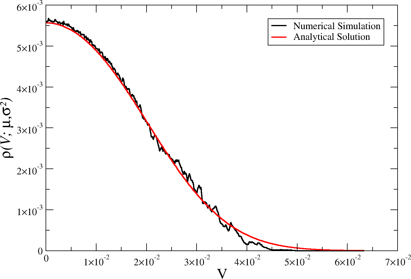
Figure 3: Comparison between the analytical solution and the experimental/numerical probability distribution of the diffusion process depicted in Fig. 2. This is the behaviour after $100$ iterations.

Fig. 3 shows how the analytical solution for the probability density given by Eq. (6) fits the numerical simulation data for the FUM. The initial conditions for the analytic curve are the same as those used in constructing Fig. 2, with $V_{0}=0.01$, $\sigma_{V_{0}}=0.001$ and $\varepsilon=0.001$. This comparison robnik2 provides a convincing verification of the analytical solution. The good fit indicates that the solution is suitable when considering an initial profile in a chaotic region and neglecting the anomalous diffusion phenomena around KAM islands.

Having obtained this solution, we need to calculate the average as $\langle V\rangle=\int_{0}^{V_{\rm f}}x\rho(V;\mu,\sigma^{2})dV$ in order to be able to predict analytically the average behaviour of the velocity. Because of the lack of symmetry, this calculation is non-trivial but, integrating between the upper and lower limits using the Jacobi Theta function representation jacobi , we find that the solution can be written as

$$\langle V\rangle=\frac{1}{2A\sqrt{\pi}}\sum_{m=-\infty}^{\infty}\sqrt{2\sigma^{2}}(\Delta^{(1)}\text{exp}+\Delta^{(2)}\text{exp})\\ +\sqrt{\pi}\left[(2mV_{\rm f}-\mu)\Delta^{(1)}\text{erf}+(2mV_{\rm f}+\mu)\Delta^{(2)}\text{erf}\right]~{},$$ (7)

where

$$\Delta^{(1)}\text{exp} = \exp\left(-\left(\frac{\mu-2mV_{\rm f}}{\sqrt{2\sigma^{2}}}\right)^{2}\right)-\exp\left(-\left(\frac{\mu-2mV_{\rm f}+V_{\rm f}}{\sqrt{2\sigma^{2}}}\right)^{2}\right),$$

$$\Delta^{(2)}\text{exp} = \exp\left(-\left(\frac{\mu+2mV_{\rm f}}{\sqrt{2\sigma^{2}}}\right)^{2}\right)-\exp\left(-\left(\frac{\mu+2mV_{\rm f}-V_{\rm f}}{\sqrt{2\sigma^{2}}}\right)^{2}\right),$$

$$\Delta^{(1)}\text{erf} = \text{erf}\left(\frac{\mu-2mV_{\rm f}-V_{\rm f}}{\sqrt{2\sigma^{2}}}\right)-\text{erf}\left(\frac{\mu-2mV_{\rm f}}{\sqrt{2\sigma^{2}}}\right),$$

$$\Delta^{(2)}\text{erf} = \text{erf}\left(\frac{\mu+2mV_{\rm f}}{\sqrt{2\sigma^{2}}}\right)-\text{erf}\left(\frac{\mu+2mV_{\rm f}+V_{\rm f}}{\sqrt{2\sigma^{2}}}\right).$$

Defining an important auxiliary variable $z=\frac{\mu}{\sqrt{2\sigma^{2}}}$ and a new parameter $\tilde{v}=\frac{V_{\rm f}}{\sqrt{2\sigma^{2}}}$ making the necessary re-arrangements, the average velocity within the FUM is given analytically by

$$\langle V\rangle=\frac{\mu}{2A}\sum_{m=-\infty}^{\infty}\frac{1}{z\sqrt{\pi}}(\Delta^{(1)}\text{exp}+\Delta^{(2)}\text{exp})\\ +\frac{1}{\mu}\left[\left(\frac{2mV_{\rm f}}{\sqrt{2\sigma^{2}}}-\mu\right)\Delta^{(1)}\text{erf}+\left(\frac{2mV_{\rm f}}{\sqrt{2\sigma^{2}}}+\mu\right)\Delta^{(2)}\text{erf}\right]~{},$$ (8)

with $A=\sum_{m=-\infty}^{\infty}\text{erf}\left(z-\frac{2mV_{\rm f}}{\sqrt{2\sigma^{2}}}\right)-\text{erf}\left(z-\tilde{v}-\frac{2mV_{\rm f}}{\sqrt{2\sigma^{2}}}\right)-\text{erf}\left(z+\frac{2mV_{f}}{\sqrt{2\sigma^{2}}}\right)+\text{erf}\left(z+\tilde{v}+\frac{2mV_{\rm f}}{\sqrt{2\sigma^{2}}}\right)$ and

$$\Delta^{(1)}\text{exp} = e^{-\left(z-\frac{2mV_{\rm f}}{\sqrt{2\sigma^{2}}}\right)^{2}}-e^{-\left(z-\frac{2mV_{\rm f}}{\sqrt{2\sigma^{2}}}+\tilde{v}\right)^{2}},$$

$$\Delta^{(2)}\text{exp} = e^{-\left(z+\frac{2mV_{\rm f}}{\sqrt{2\sigma^{2}}}\right)^{2}}-e^{-\left(z+\frac{2mV_{\rm f}}{\sqrt{2\sigma^{2}}}-\tilde{v}\right)^{2}},$$

$$\Delta^{(1)}\text{erf} = \text{erf}\left(z-\frac{2mV_{f}}{\sqrt{2\sigma^{2}}}+\tilde{v}\right)-\text{erf}\left(z-\frac{2mV_{\rm f}}{\sqrt{2\sigma^{2}}}\right),$$

$$\Delta^{(2)}\text{erf} = \text{erf}\left(z+\frac{2mV_{\rm f}}{\sqrt{2\sigma^{2}}}\right)-\text{erf}\left(z+\frac{2mV_{\rm f}}{\sqrt{2\sigma^{2}}}+\tilde{v}\right).$$

Furthermore, the mean $\mu$ and variance $\sigma^{2}$ are calculated, by construction, over the point charge, which is characterised by an unbounded diffusion process. According to our initial mapping, Eq. (1), the point charge mapping is given by $V_{n+1}=V_{n}-2\varepsilon\sin(\phi)$, where $\phi$ is an uniform random variable, as observed in Fig. 2, it is then possible to write the mean and variance for the point charge as

$$\begin{split}\mu_{n+1}&=\langle V_{n+1}\rangle=\langle V_{n}\rangle\Rightarrow\mu=\mu_{0}=V_{0}\\ \sigma^{2}_{n+1}&=\langle V^{2}_{n+1}\rangle-\langle V_{n+1}\rangle^{2}=\langle V^{2}_{n}\rangle+2\varepsilon^{2}-\langle V_{n}\rangle^{2}\\ &\Rightarrow\sigma^{2}_{n+1}=\sigma^{2}_{n}+2\varepsilon^{2}~{}.\end{split}$$

Following the theory of difference equations aprox , assuming a large number of iterations and small values of $\varepsilon$, it is then possible to write $\sigma$ as a function of $n$

$$\sigma^{2}_{n+1}-\sigma^{2}_{n}=\frac{d\sigma^{2}}{dn}~{}\Rightarrow~{}\sigma^{2}(n)=\sigma^{2}_{0}+2\varepsilon^{2}n~{}.$$

This result is important because it carries the information that the variance is a function of the number of iterations $\sigma^{2}=\sigma^{2}(n)$, connecting the solution of the diffusion equation to the discrete mapping of the FUM. Moreover, the initial variance $\sigma_{0}$ is zero if the initial profile is considered a perfect Dirac delta function. This also tells us the diffusion is normal, since $\sigma\propto\sqrt{n}$. In addition, it is also possible to calculate the diffusion coefficient, which is a constant and quite intuitive with our suppositions for this case, so that $D=\epsilon^{2}$. Then $z$ is also a function of the number of iterations $n$ such that

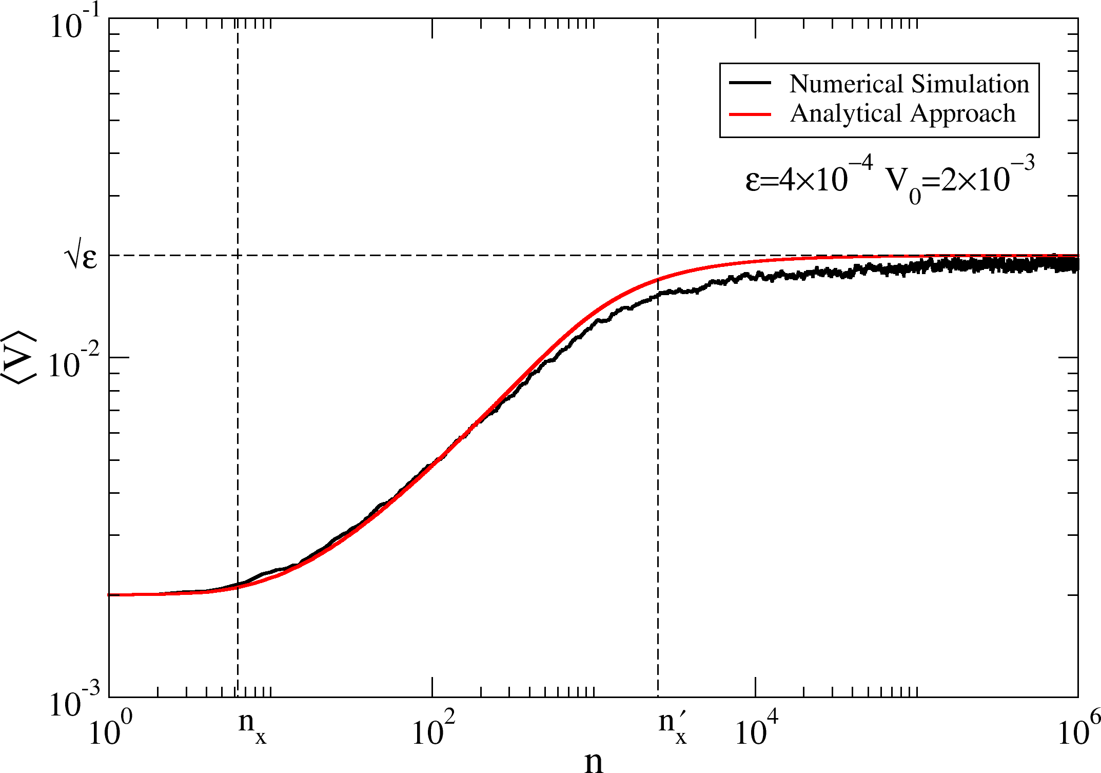
Figure 4: (colour online). The average velocity $\langle V\rangle$ of particles in the FUM showing its evolution with the number of iterations $n$. With parameter $\varepsilon=4\times 10^{-4}$ an ensemble of $10^{3}$ particles, each with $V_{0}=2\times 10^{-3}$ was iterated until there had been $10^{6}$ collisions. The numerical simulations (rough black line) are compared with the analytic theory (smooth red line). Note the saturation of $\langle V\rangle$ towards $\sqrt{\varepsilon}$ that occurs at large $n$ in both theory and simulation.

$$z=\frac{\mu}{\sqrt{2}\sigma(n)}~{}\Rightarrow~{}z(n)=\frac{V_{0}}{2\varepsilon\sqrt{n}}~{}.$$ (9)

Substituting Eq. (9) into Eq. (8), we can calculate how the average velocity behaves as a function of the number of iterations for the dynamics of the FUM. But of course we now need to check whether, or not, this theory really describes the actual behaviour of the average velocity.

IV Analytical $\times$ Numerical results

Fig. 4 compares the numerical simulation data with the analytic predictions of Eqs. (8),(9). The expression for $\langle V\rangle$, given by Eq. (8), represents a continuous competition between the exponential and error functions, so it is interesting to study their arguments. Based on a graphical analysis, we conclude that there are two changes of behaviour: at $z=1$; and at $\tilde{v}=1$. First, taking $z=1$

$$z=1~{}\Rightarrow~{}\frac{V_{0}}{2\varepsilon\sqrt{n}}=1~{}\Rightarrow~{}n=\left(\frac{V_{0}}{2\varepsilon}\right)^{2}~{}\Rightarrow~{}n=\frac{V_{0}^{2}}{4\varepsilon^{2}}~{},$$

but in this case, $n=n_{x}$ marking the first crossover . Thus

$$n_{x}=\frac{V_{0}^{2}}{4\varepsilon^{2}}~{}.$$ (10)

Secondly, taking $\tilde{v}=1$

$$\tilde{v}=1~{}\Rightarrow~{}\frac{V_{\rm f}}{2\varepsilon\sqrt{n}}=1~{}\Rightarrow~{}n\approx\left(\frac{2\sqrt{\varepsilon}}{2\varepsilon}\right)^{2}~{}\Rightarrow~{}n\approx\frac{1}{\varepsilon}~{},$$

but now, $n=n^{\prime}_{x}$ marking the second crossover. Thus

$$n^{\prime}_{x}\approx\frac{1}{\varepsilon}~{}.$$ (11)

Another important result is the limit

$$\lim_{\sigma\rightarrow\infty}\langle V\rangle=\lim_{n\rightarrow\infty}\langle V\rangle=\frac{V_{\rm f}}{2}\approx\sqrt{\varepsilon}~{},$$ (12)

which provides the saturation value $V_{sat}$. Then, Fig. 4 shows the average velocity for an ensemble of $10^{3}$ particles, all with initial velocity $V_{0}=2\times 10^{-3}$, taken within the interval $\phi_{0}\in[0,2\pi]$. The analytical predictions for the first crossover $n_{x}$, Eq. (10), the second crossover $n^{\prime}_{x}$, Eq. (11), and the saturation plateau when $n\rightarrow\infty$, Eq. (12), are shown by the dashed lines.

The analytical approach, yielding Eq. (8), clearly agrees well with the numerical simulation data. The correspondence might have been even closer were if not for the fact that the diffusion is not ideal for higher values of $V$, due to the configuration of the phase space. This also explains the fluctuation for $n>n^{\prime}_{x}$. The diffusion around stability structures like KAM islands leads to the very complicated behaviour known as anomalous diffusion. However, the associated stickiness of the dynamics near the islands, though real, is a relatively minor effect given the size of the whole phase space: Harsoula et al harsoula conclude that, for a long enough interval, averaging over the ensemble smooths the observables so that the stickiness can largely be neglected.

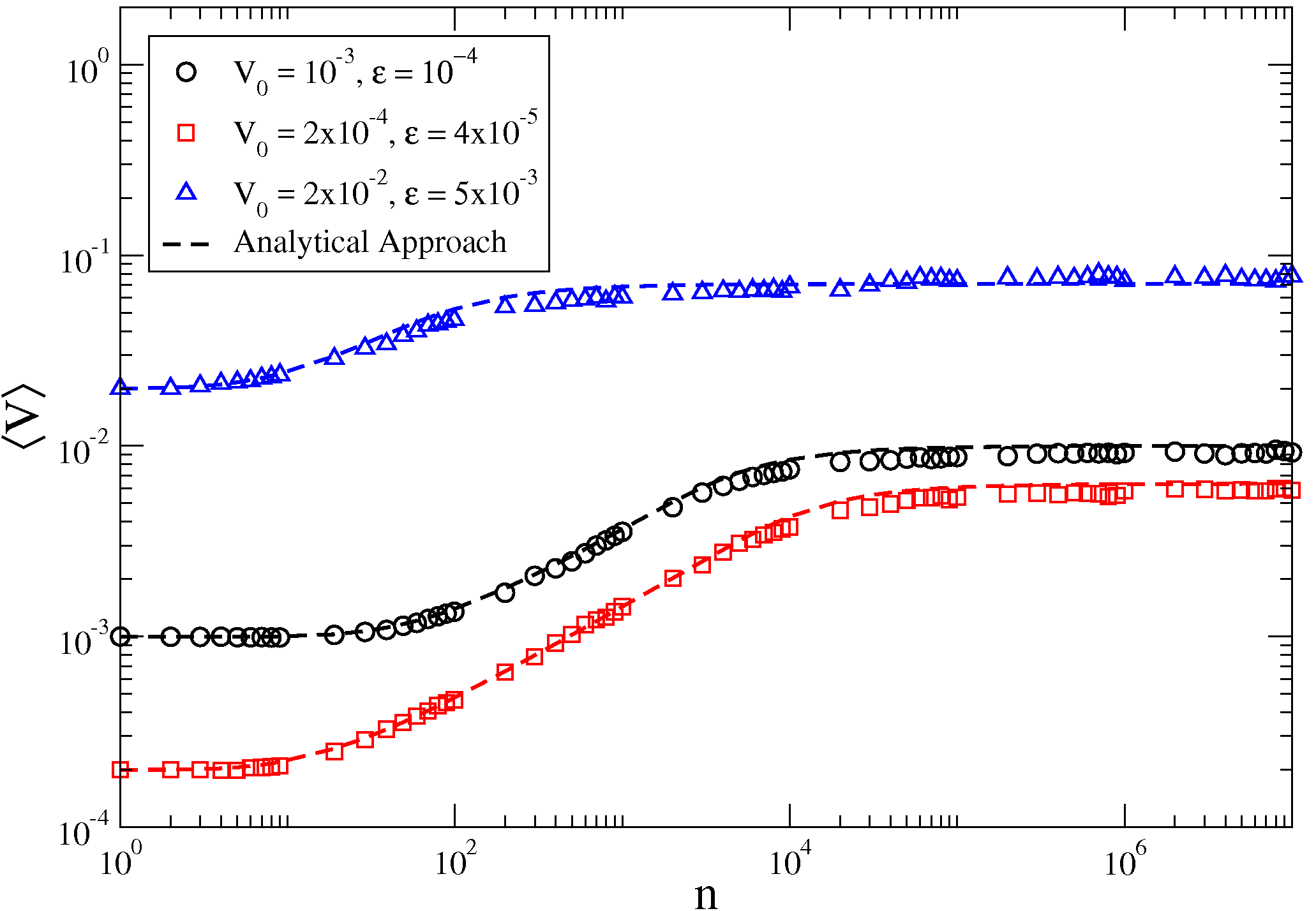
Figure 5: (colour online). The average velocity $\langle V\rangle$ of particles in the FUM showing how it evolves with the number of iterations $n$, under different conditions. The analytic theory (dashed lines) is compared with numerical simulations (data points) for three different initial velocities $V_{0}$ and values of the control parameter $\varepsilon$, as listed in the inset. In each case, the simulations involved an ensemble of $10^{4}$ particles iterated up to $10^{7}$ collisions.

Fig. 5 shows compares numerical data with the corresponding analytical predictions for three different initial velocities $V_{0}$ and values of the control parameter $\varepsilon$. It is important to remember that the position of the upper boundary in the phase space, which is the first invariant spanning curve, is approximated by $V_{\rm f}\approx 2\sqrt{\varepsilon}$. Then, for each value of the parameter $\varepsilon$, a different bounded phase space is considered. Again, it is evident that the analytic curves provide an excellent fit to the numerical data, even for relatively large values of $\varepsilon$.

We emphasize that Eqs. (10, 11, 12) represent the first analytic predictions to be made for the Fermi-Ulam model. They agree well with what was proposed on purely empirical grounds prl2004 more than a decade ago. Three hypotheses were then proposed, based on a scaling analysis: (i) $n_{x}\propto\frac{V_{0}^{2}}{\varepsilon^{2}}$ which agrees perfectly with Eq. (10), and we now also obtain the proportionality constant $\frac{1}{4}$; in addition (ii) $n^{\prime}_{x}\propto\frac{1}{\varepsilon}$ which agrees with Eq. (11); and finally (iii) $V_{sat}\propto\varepsilon^{\alpha}$, with $\alpha\approx\frac{1}{2}$, which agrees with Eq. (12).

V Conclusion

We conclude that a combination of the theory of diffusive processes with dynamical systems theory, plus the method of images from electrostatics, provides a powerful method for treating systems described by nonlinear mappings. The method can be expected to work for mixed phase spaces that are delimited by boundaries through which there are no fluxes. Application to the Fermi-Ulam model, taken as an example, has yielded some interesting features and excellent agreement both with numerical simulations and with earlier empirically-based theoretical considerations. Extension of the procedure discussed here to time-dependent billiards gelfreich is an interesting possibility for future work.

- (1) A. J. Lichtenberg, M. A. Lieberman. Regular and Chaotic Dynamics, Springer (1992).
- (2) E. Ott, Phys. Rev. Lett. 42, 1628 (1979).
- (3) B. V.Chirikov. A universal instability of many-dimensional oscillator systems, Phys. Rep. 52, 263 (1979).
- (4) R. Venegeroles, Phys. Rev. Lett. 101, 054102 (2008).
- (5) G. M. Zaslasvsky, Physics of Chaos in Hamiltonian Systens, Imperial College Press (2007).
- (6) T. Manos, M. Robnik, Phys. Rev. E 89, 022905 (2014).
- (7) R. Venegeroles, Phys. Rev. Lett. 102, 064101 (2009).
- (8) O. Alus, S. Fishman and J. D. Meiss, Phys. Rev. E 96, 032204 (2017).
- (9) R. M. da Silva, M. W. Beims, C. Manchein, Phys. Rev. E 92, 022921 (2015).
- (10) P. J. Basser, D. K. Jones, NMR in Biomedicine 15, 07 (2002).
- (11) H. A. Kramers, Physica, 7 284 (1940).
- (12) J. D. Meiss, Chaos 25, 097602 (2015).
- (13) E. G. Altmann, J. S. E. Portela and T. Tél, Rev. Mod. Phys. 85, 869 (2013).
- (14) G. M. Zaslavsky, Physics Reports 371, 461 (2002).
- (15) M. A. Lieberman and A. J. Lichtenberg, Phys. Rev. A 5, 1852 (1971).
- (16) E. Fermi, Phys. Rev. 75, 1169 (1949).
- (17) Suppose that the oscillating wall is fixed, however when the particle suffers a collision, it exchanges momentum as if the wall were moving. This simplified version is indeed valid when the nonlinear parameter is relatively small.
- (18) T. Pereira, D. Turaev, Phys. Rev. E 91, 010901 (2015).
- (19) E. D. Leonel, J. A. Oliveira, F. Saif, J. Phys. A 44, 302001 (2011).
- (20) J. Crank. The Mathematics of Diffusion, Oxford University Press (1975).
- (21) H. Shore, Communications in Statistics – Theory and Methods 34, 507 (2005).
- (22) J. M. Rohrbasser, J. Véron, Population 58, 303 (2003).
- (23) K. Pearson, Biometrika 13, 25 (1920).
- (24) Črt Lozej and Marko Robnik, Phys. Rev. E 97, 012206 (2018).
- (25) J. M. Borwein and P. B. Borwein, Pi and the AGM: A Study in Analytic Number Theory and Computational Complexity, Wiley (1987).
- (26) C. M. Bender, S. A. Orszag, Advanced Mathematical Methods for Scientists and Engineers I: Asymptotic Methods and Perturbation Theory, Springer (1999)
- (27) M. Harsoula, K. Karamanos and G. Contopoulos, Phys. Rev. E 99, 032203 (2019).
- (28) E. D. Leonel, P. V. E. McClintock and J. K. L. da Silva, Phys. Rev. Lett. 93, 014101 (2004).
- (29) K. Shah, V. Gelfreich, V. Rom-Kedar and D. Turaev, Phys. Rev. E 91, 062920 (2015).