Solving the one-dimensional Ising chain via mathematical induction: An intuitive approach to the transfer matrix

Abstract

The aim of this work is to present a formulation to solve the one-dimensional Ising model using the elementary technique of mathematical induction. This formulation is physically clear and leads to the same partition function form as the transfer matrix method, which is a common subject in the introductory courses of statistical mechanics. In this way our formulation is a useful tool to complement the traditional more abstract transfer matrix method. The method can be straightforwardly generalized to other short-range chains, coupled chains and is also computationally friendly. These two approaches provide a more complete understanding of the system, and therefore our work can be of broad interest for undergraduate teaching in statistical mechanics.

I Introduction

The one-dimensional (1D) Ising model Ising (1925); Brush (1967) is of fundamental importance in an introductory course on statistical mechanics, because it is connected to many interesting physical concepts; see e.g. Ref. Taroni (2015) for a recent entertaining introduction. Despite the absence of a genuine phase transition, the 1D Ising model still plays a central role in the comprehension of many principles, phenomena, and numerical methods in statistical physics. Indeed, the model itself and its large number of variations have become the most common conceptual platform to which discussions are constantly referred to. Consequently, in the context of teaching, the development of an intuitive comprehension of the many features of the Ising and related models is an instrumental tool for the proper acquisition of the subsequent content. Moreover, while the exact solution of the 2D version of the model is a very challenging exercise Onsager (1944); Kac and Ward (1952); Kanô and Naya (1953); Domb (1960), the one-dimensional calculation typically becomes for the students the first contact with an exactly solvable many body model at their reach. In this way facing a decades-old scientific problem which, with slight modifications, can easily turn on current interest J.Kofinger and Dellago (2010); Sarkanych et al. (2018); Strečka et al. (2008); Bach et al. (2019). There exist several analytical methods to solve the 1D Ising model, some of them providing novel approaches and interesting view points Baxter (1982); Seth (2017). However, the transfer matrix method is by far the most extended technique in undergraduate lectures, due in part to its wide general use across many physical subjects Moreno et al. (2005); Pujol and Pérez (2007); Pujol et al. (2014); Zad and Ananikian (2017); Torrico et al. (2018). The method is simple to use and can be flexibly generalized to cover other interesting models as next-nearest neighbours Kassan-Ogly (2001); Tenga et al. (2002), Potts spins Shrock and Tsai (1997); Shrock and Xu (2010) and coupled chains Yurishchev (2001); Guidi et al. (2015).

There is, though, a common conceptual barrier from novice students to properly understand the basis of the transfer matrix method, unless the students are comfortable with the bond representation. The latter is unfortunately not always the case as this is usually their first encounter with the Ising model. In this line, many teachers find the physical basis of the regular transfer matrix method a bit uneasy to define and explain. In many cases, after getting familiar with the method, the lack of an axiomatic presentation of the matrix or even an intuitive analogy makes it to be generally seen as a lucky trick whose underlying idea has no link with the physical problem. It is expectable that efforts in the direction of offering physical connections to this trick can be very welcomed in the wide community of statistical physics students and teachers. In this paper we show that, by using elementary mathematical induction, it is possible to solve the 1D Ising model using simple mathematics where mathematical reduction can be seen from the very first step. More importantly, we find a working transformation from which the transfer matrix result can be derived. The advantage of this formulation is that: (1) it is very physically clear and mathematically simple, and (2) it connects the transfer matrix method with an intuitively logical mechanism. We believe this derivation could be very useful for developing the intuitive comprehension of this topic in introductory lectures of statistical mechanics.

II The Transfer Matrix Method

We start by a quick review of the regular transfer matrix method. In the presence of an external field, the 1D Ising Hamiltonian takes the form

$$H=-J\sum_{i=1}^{N}S_{i}S_{i+1}-h\sum_{i=1}^{N}S_{i},$$ (1)

where $N$ spins $S_{i}=\pm 1$ are placed in a chain, interacting only with their nearest neighbours and with the external field $h$. Periodic boundary conditions are imposed by setting $S_{N+1}\equiv S_{1}$.

The canonical partition function for this system can be expressed as

$$Z_{N}=\sum_{\{S_{i}\}}e^{-\beta H(S_{1},S_{2},\ldots,S_{N})}=\sum_{\{S_{i}\}}e^{\beta\big{[}\sum_{i=1}^{N}JS_{i}S_{i+1}+\frac{1}{2}h\sum_{i=1}^{N}(S_{i}+S_{i+1})\big{]}},$$ (2)

where $\{S_{i}\}$ means that the sum runs over all ($2^{N}$) possible combination of the values of the $N$ variables $S_{i}$, i.e., over all possible states of the system. The next step is to use the bond representation and factor the Boltzmann weights to pairwise factors, a decomposition of the bonds

$$Z_{N}=\sum_{S_{1}}\sum_{S_{2}}\cdots\sum_{S_{N}}\prod_{i=1}^{N}e^{\beta\big{[}JS_{i}S_{i+1}+\frac{1}{2}h(S_{i}+S_{i+1})\big{]}}.$$ (3)

Introducing a matrix, the transfer matrix, with the corresponding matrix elements from the factors defined as

$$P_{S_{i}S_{j}}=e^{\beta JS_{i}S_{j}+\frac{1}{2}\beta h(S_{i}+S_{j})},$$ (4)

the partition function can be written as

$$Z_{N} = \sum_{S_{1}}\sum_{S_{2}}\cdots\sum_{S_{N}}P_{S_{1}S_{2}}P_{S_{2}S_{3}}\cdots P_{S_{N}S_{1}}$$ (5)

$$= \sum_{S_{1}}(P^{N})_{S_{1}S_{1}}=Tr(P^{N}).$$

It is important to realize that there is no matrix in the partition function itself, only matrix elements. The summations remarkably happen to resemble matrix multiplications. The approach is not very intuitive, mostly because it is difficult to see a priori that this reduction will take place, at least for the first time, and the students have to take the fact that it works. As we will demonstrate in the next section, this same result can be obtained by means of a physically intuitive formalism, where reduction can be seen in the first place.

Before ending this section, we summarize some important results here for reference. The matrix $P$ is a $2\times 2$ matrix as the variables $S_{i}$ has two possible values. Ordering the spins in the state space as $1$ and $-1$, the matrix reads

$$P=\begin{pmatrix}e^{\beta(J+h)}&e^{-\beta J}\\ e^{-\beta J}&e^{\beta(J-h)}\end{pmatrix}$$ (6)

The partition function can be calculated as

$$Z_{N}=Tr(P^{N}) = \lambda_{1}^{N}+\lambda_{2}^{N},$$ (7)

where $\lambda_{1}$ and $\lambda_{2}$ are the eigenvalues of the matrix $P$, satisfying the usual characteristic equation

$$\lambda^{2}-Tr(P)\lambda+Det(P)=0$$ (8)

with solutions

$$\lambda_{1,2}=e^{\beta J}\left[\mathrm{cosh}(\beta h)\pm\sqrt{\mathrm{sinh}^{2}(\beta h)+e^{-4\beta J}}\right],$$ (9)

where $\lambda_{1}>\lambda_{2}$ for any value of $h$. Consequently, in the thermodynamic limit, the term involving $\lambda_{2}$ in the right hand side of Eq. (7) can be neglected

$$Z_{N} \xrightarrow[N\to\infty]{}\lambda_{1}^{N}$$ (10)

ending up with a partition function in the form

$$Z \approx\lambda_{1}^{N}=e^{N\beta J}\left[\mathrm{cosh}(\beta h)+\sqrt{\mathrm{sinh}^{2}(\beta h)+e^{-4\beta J}}\right]^{N}.$$ (11)

Importantly, the free energy $f$ and the magnetization $m$ per spin are

$$f(h,T) = -\frac{1}{N}k_{B}T\ln(Z)=-k_{B}T\ln\lambda_{1}$$ (12)

$$= -J-k_{B}T\ln\left[\mathrm{cosh}(\beta h)+\sqrt{\mathrm{sinh}^{2}(\beta h)+e^{-4\beta J}}\right],$$

$$m(h,T) = -\frac{\partial f}{\partial h}$$ (13)

$$= \frac{\sinh(\beta h)}{\sqrt{\sinh^{2}(\beta h)+e^{-4\beta J}}},$$

from which, since $\sinh(\beta h)\xrightarrow[\beta h\to 0]{}0$, it is clear that no spontaneous magnetization occurs at any finite temperature in the absence of an external field.

III Solving via Mathematical Induction

We now consider the more intuitive approach expressed in the following question: given the partition function for $N$ spins $Z_{N}$, could one construct the partition function for $N+1$ spins $Z_{N+1}$? In this situation, the new partition function $Z_{N+1}$ seems likely to be expressible in terms of the old partition function $Z_{N}$, after all, the new spin only change the interactions locally. Without loss of generality, we assume this extra spin $S_{N+1}$ is inserted at the right end of the chain, i.e., interacting with spins $S_{N}$ and $S_{1}$.

In order to keep track of the modifications raised by the new spin, we now split the configuration space in four subsets, according to the four possible orientations of the first and the last spins. This is a preparation step for mathematical induction, as we know one can adjust the Boltzmann factors properly when a new spin is added if the additional interactions (with $S_{1}$ and $S_{N}$) are fully known. All configurations with $S_{1}=S_{N}=1$ form the subset $\{\uparrow\uparrow\}$, configurations with $S_{1}=1$ and $S_{N}=-1$ form the subset $\{\uparrow\downarrow\}$, and so on, each of them has $2^{N-2}$ configurations. That is to say

$$\{S_{i}\}=\{\uparrow\uparrow\}\cup\{\uparrow\downarrow\}\cup\{\downarrow\uparrow\}\cup\{\downarrow\downarrow\}.$$ (14)

Such a splitting is illustrated in Fig. 1 A. Extending the split to the sum in the partition function, one can define four terms associated to these sectors $Z_{N}^{\uparrow\uparrow}$, $Z_{N}^{\uparrow\downarrow}$, $Z_{N}^{\downarrow\uparrow}$ and $Z_{N}^{\downarrow\downarrow}$, such that

$$Z_{N}^{\uparrow\uparrow} = \sum_{\{\uparrow\uparrow\}}e^{-\beta H(S_{1},S_{2},\ldots,S_{N})}=\sum_{\{S_{i}\}:S_{1}=S_{N}=1}e^{-\beta H(S_{1},S_{2},\ldots,S_{N})}$$ (15)

$$Z_{N}^{\uparrow\downarrow} = \sum_{\{\uparrow\downarrow\}}e^{-\beta H(S_{1},S_{2},\ldots,S_{N})}=\sum_{\{S_{i}\}:S_{1}=1,S_{N}=-1}e^{-\beta H(S_{1},S_{2},\ldots,S_{N})}$$ (16)

$$Z_{N}^{\downarrow\uparrow} = \sum_{\{\downarrow\uparrow\}}e^{-\beta H(S_{1},S_{2},\ldots,S_{N})}=\sum_{\{S_{i}\}:S_{1}=-1,S_{N}=1}e^{-\beta H(S_{1},S_{2},\ldots,S_{N})}$$ (17)

$$Z_{N}^{\downarrow\downarrow} = \sum_{\{\downarrow\downarrow\}}e^{-\beta H(S_{1},S_{2},\ldots,S_{N})}=\sum_{\{S_{i}\}:S_{1}=S_{N}=-1}e^{-\beta H(S_{1},S_{2},\ldots,S_{N})}$$ (18)

and the partition function can be expressed as

$$Z_{N}=Z_{N}^{\uparrow\uparrow}+Z_{N}^{\uparrow\downarrow}+Z_{N}^{\downarrow\uparrow}+Z_{N}^{\downarrow\downarrow}.$$ (19)

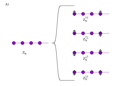
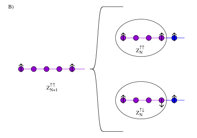
Figure 1: Schematic representation of the configuration space. Spins (circles) with no explicit orientation can take any of the two values $\pm 1$, and extra bonds at the right of the chain indicates periodic interactions. Panel A: the configuration space of a chain of $N=4$ spins is decomposed in four sets of configurations by considering the four possible orientations of the spins at the extremes. Panel B: for a chain of $N+1=5$ spins, the subset $(\uparrow\uparrow)$ is the union of the subsets $(\uparrow\uparrow)$ and $(\uparrow\downarrow)$ of the chain with $N=4$ spins, plus an extra spin $S_{N+1}=1$.

The next step is to explicitly find the transformations of each component of the partition function when going from a system of $N$ spins to $N+1$ spins. Since the new spin is inserted at the right end, it is clear, for instance, that the subset $\{\uparrow\uparrow\}$ of the new $N+1$ system will emerge from the union of the sets $\{\uparrow\uparrow\}$ and $\{\uparrow\downarrow\}$ of the $N$-spin chain with an extra spin up $S_{N+1}=1$. This case is shown schematically in Fig. 1 B. Consequently, the new term $Z_{N+1}^{\uparrow\uparrow}$ will have two contributions, one involving $Z_{N}^{\uparrow\uparrow}$ and the other involving $Z_{N}^{\uparrow\downarrow}$. The first contribution comes from adding a spin $+1$ at the site $N+1$ to the previous set $\{\uparrow\uparrow\}$. The second contribution comes from adding a spin $+1$ at the site $N+1$ to the previous set $\{\uparrow\downarrow\}$.

$$Z_{N+1}^{\uparrow\uparrow}=c_{1}Z_{N}^{\uparrow\uparrow}+c_{2}Z_{N}^{\uparrow\downarrow},$$ (20)

where $c_{1}$ and $c_{2}$ are proper modifications to the Boltzmann weights.

The factors can be written down very simply. For example, in the first term, a new spin up is added, which contributes a factor $\exp(\beta h)$ from interactions with the field, two new satisfied bonds are created and one satisfied bond is eliminated, this contributes to a factor $\exp(\beta J)$. Putting the magnetic and bond contributions together, $c_{1}=\exp(\beta(h+J))$. Similarly, $c_{2}=\exp(\beta(h+J))$ as well. The whole transformation can be simply enumerated, introducing for simplicity a vector partition function

$$\vec{z}_{N}=\begin{pmatrix}Z_{N}^{\uparrow\uparrow},Z_{N}^{\uparrow\downarrow},Z_{N}^{\downarrow\uparrow},Z_{N}^{\downarrow\downarrow}\end{pmatrix}^{T},$$ (21)

in such a way that the partition function of the system can be expressed as a summation reduction $Z_{N}=\sum(\vec{z}_{N})$. And the recurrence relation can be expressed concisely in the form

$$\vec{z}_{N+1} = M\vec{z}_{N},$$ (22)

where the recurrence matrix $M$ is

$$M=\begin{pmatrix}e^{\beta(J+h)}&e^{\beta(J+h)}&0&0\\ e^{-\beta(3J+h)}&e^{\beta(J-h)}&0&0\\ 0&0&e^{\beta(J+h)}&e^{-\beta(3J-h)}\\ 0&0&e^{\beta(J-h)}&e^{\beta(J-h)}\end{pmatrix}$$ (23)

Note that in spite of the matrix is $4\times 4$ compared with the transfer matrix, it is block diagonal. Indeed we will see in the following the partition function, upon summation reduction, takes exactly the same form as that of the transfer matrix method. And most importantly for the learning context, the derivation of this recurrent relation is absolutely intuitive, it comes just from considering the energetic effect of inserting a new spin in the chain. This is the most important step of the method, the rest is straightforward algebraic calculations.

Next the job is to find the vector partition function for a small system to start the induction e.g. a two-spin system. It is natural to start from $N=2$, however, one can check that it is also possible to start from $N=1$, i.e., a single spin on a ring which loops over and interact with itself. In this case we have

$$\vec{z}_{1}=\begin{pmatrix}\exp(\beta(J+h)),0,0,\exp(\beta(J-h))\end{pmatrix}^{T}.$$ (24)

Therefore, we readily have $\vec{z}_{N}=M^{N-1}\vec{z}_{1}$. As $M$ is a block diagonal matrix, let us call $M_{11}$ and $M_{22}$ to the first and last non-zero blocks respectively, we then write

$$\vec{z}_{N} = \begin{pmatrix}M_{11}^{N-1}&0\\ 0&M_{22}^{N-1}\end{pmatrix}\vec{z}_{1}$$ (25)

$$= \begin{pmatrix}M_{11}^{N-1}\vec{z}_{1}(1:2)\\ M_{22}^{N-1}\vec{z}_{1}(3:4)\end{pmatrix},$$ (26)

where $\vec{u}(m:n)$ is the vector formed by the elements from $m$-th to $n$-th of the vector $\vec{u}$. Naturally,

$$Z_{N} = \sum(\vec{z}_{N})=\sum(\vec{z}_{N}(1:2))+\sum(\vec{z}_{N}(3:4)).$$ (27)

Note that we are going in this step from a $4\times 4$ matrix towards a $2\times 2$ matrix upon the summation reduction, the same matrix size as the transfer matrix.

Now we introduce a lemma which is easy to prove:

Lemma: If $A$ is a $2\times 2$ matrix and $b$ is a $2\times 1$ vector, then $\sum(Ab)=Tr(A\times[b,b])$.

Therefore,

$$Z_{N} = Tr\left(M_{11}^{N-1}[\vec{z}_{1}(1:2),\vec{z}_{1}(1:2)]\right)+Tr\left(M_{22}^{N-1}[\vec{z}_{1}(3:4),\vec{z}_{1}(3:4)]\right)$$ (28)

$$= Tr\left(M_{11}^{N-1}[\vec{z}_{1}(1:2),\vec{z}_{1}(1:2)]+M_{22}^{N-1}[\vec{z}_{1}(3:4),\vec{z}_{1}(3:4)]\right).$$ (29)

Both $M_{11}$ and $M_{22}$ can be easily symmetrized using similarity transformations

$$M_{11} = \begin{pmatrix}e^{\beta(J+h/2)}&0\\ 0&e^{-\beta(J+h/2)}\end{pmatrix}\begin{pmatrix}e^{\beta(J+h)}&e^{-\beta J}\\ e^{-\beta J}&e^{\beta(J-h)}\end{pmatrix}\begin{pmatrix}e^{-\beta(J+h/2)}&0\\ 0&e^{\beta(J+h/2)}\end{pmatrix}$$ (30)

$$M_{22} = \begin{pmatrix}e^{-\beta(J-h/2)}&0\\ 0&e^{\beta(J-h/2)}\end{pmatrix}\begin{pmatrix}e^{\beta(J+h)}&e^{-\beta J}\\ e^{-\beta J}&e^{\beta(J-h)}\end{pmatrix}\begin{pmatrix}e^{\beta(J-h/2)}&0\\ 0&e^{-\beta(J-h/2)}\end{pmatrix}$$ (31)

Plugging these two equations to $Z_{N}$, Eq. 29 remarkably simplifies to

$$Z_{N}=Tr\begin{pmatrix}e^{\beta(J+h)}&e^{-\beta J}\\ e^{-\beta J}&e^{\beta(J-h)}\end{pmatrix}^{N},$$ (32)

which is identical to the transfer matrix result in Eq. (5).

Finally, we mention that the method can also be used in a purely numerical manner directly from the recurrence relation. This is computationally appealing because the setup is straightforward, and it can be easily applied to e.g. free boundary conditions. While this may seem unnecessary for our example, the method can be readily generalized to disordered systems such as random ferromagnets Theodorou (1982); Avgin (1996) and even spin glasses Edwards and Anderson (1975); Machta (2010) with competing interactions.

IV Conclusions

In this work, we have presented a mathematical induction approach to the solution of the 1D Ising model, complementing the more traditional transfer matrix method. The analytical procedure is rather intuitive, physically clear, and computationally friendly, which makes the formalism very suited to be used in introductory statistical mechanics courses. Remarkably, the algebraic derivation following this path connects with the formalism of the transfer matrix method. This fully equivalence is an extra benefit since it provides a physical interpretation of the transfer matrix, that appears naturally from considering the recurrent summation of the energetic cost of inserting a new spin in the chain.