Metallicity of the star formation based on the observational properties of star forming galaxies

Metallicity of stars formed throughout the cosmic history based on the observational properties of star forming galaxies

Abstract

Metallicity is one of the crucial factors that determine stellar evolution. To characterize the properties of stellar populations one needs to know the fraction of stars forming at different metallicities. Knowing how this fraction evolves over time is necessary e.g. to estimate the rates of occurrence of any stellar evolution related phenomena (e.g. double compact object mergers, gamma ray bursts). Such theoretical estimates can be confronted with observational limits to validate the assumptions about the evolution of the progenitor system leading to a certain transient. However, to perform the comparison correctly one needs to know the uncertainties related to the assumed star formation history and chemical evolution of the Universe.
We combine the empirical scaling relations and other observational properties of the star forming galaxies to construct the distribution of the cosmic star formation rate density at different metallicities and redshifts. We address the question of uncertainty of this distribution due to currently unresolved questions, such as the absolute metallicity scale, the flattening in the star formation$-$mass relation or the low mass end of the galaxy mass function. We find that the fraction of stellar mass formed at metallicities <10% solar (>solar) since z=3 varies by $\sim$18% ($\sim$26%) between the extreme cases considered in our study. This uncertainty stems primarily from the differences in the mass metallicity relations obtained with different methods. We confront our results with the local core-collapse supernovae observations. Our model is publicly available.

1 Introduction

The distribution of the star formation over metallicities varies throughout the history of the Universe. It is an important ingredient to estimate the rate of occurrence of any stellar or binary evolution related phenomena, such as different types of supernovae, double compact object mergers or gamma ray bursts (e.g. Langer & Norman, 2006; Dominik et al., 2013; Belczynski et al., 2016; Mapelli et al., 2017; Chruslinska et al., 2019; Eldridge et al., 2019). Such theoretical estimates can be, for instance, confronted with observational determinations of rates to validate the assumptions about the evolution of the progenitor star or system leading to a certain type of transient. However, to perform the comparison correctly, one needs to know the uncertainties related to the assumed star formation history and chemical evolution of the Universe. This is especially important in the case of transients whose formation scenarios are particularly sensitive to metallicity, e.g. long gamma ray bursts (long GRB) and stellar double black hole mergers, both forming much more efficiently at low metallicities ($\lesssim$0.1 solar metallicity; see e.g. Langer & Norman (2006), Stanek et al. (2006), Woosley & Heger (2006), Palmerio et al. (2019) for long GRB and e.g. Belczynski et al. (2010), Eldridge & Stanway (2016), Stevenson et al. (2017), Giacobbo et al. (2018), Klencki et al. (2018) for double black hole mergers).
Recently, Chruslinska et al. (2019) demonstrated that the merger rate density of double black holes estimated for the same description of the evolution of their progenitor systems can be significantly different (even by a factor of $\sim$10) depending on the assumed distribution of the cosmic star formation rate density at different metallicities and time (probed by redshift; $SFRD(Z,z)$). This underlines the need for a better constrained picture of the star formation history and chemical evolution of the Universe and of understanding the associated uncertainties.
So far different groups have taken different approaches to determine the $SFRD(Z,z)$, often combining observations, theoretical inferences and/or cosmological simulations (e.g. Langer & Norman, 2006; Niino, 2011; Dominik et al., 2013; Belczynski et al., 2016; Lamberts et al., 2016; Mapelli et al., 2017; Schneider et al., 2017).
In this paper we combine the empirical scaling relations from various observational studies describing the properties of star forming galaxies (star formation rate, mass, metallicity) to construct the distribution of the cosmic star formation rate density at different metallicities and time/redshift. Our method is outlined in Sec. 3. We also address the question of the uncertainty of this distribution, given the currently unresolved problems (discussed in detail in Sec. 2), such as the absolute metallicity scale (e.g. Kewley & Ellison, 2008) or the flattening (or lack of it) at the high mass part of the star formation mass relation (e.g. Speagle et al., 2014; Lee et al., 2015). Systematic evaluation of these uncertainties in the context of $SFRD(Z,z)$ is still lacking in the literature.
Our results are summarized in Sec. 4. In Sec. 5 we apply them to calculate the volumetric core-collapse supernovae rate and their local rate as a function of metallicity and contrast those quantities with observations. We discuss the reliability of our results at high redshifts and present a brief comparison with simulations and earlier studies in Sec. 6.
The results of our calculations are publicly available at https://ftp.science.ru.nl/astro/mchruslinska/. They can be applied to calculate the cosmological rates of various stellar evolution related events and to asses their uncertainty due to uncertainties in observationally inferred $SFRD(Z,z)$. They can also be contrasted with the results from cosmological simulations.
Where appropriate we adopt a standard flat cosmology with $\Omega_{M}$=0.3, $\Omega_{\Lambda}$=0.7 and H${}_{0}=70\rm\ km\ s^{-1}\ Mpc^{-1}$ and assume a Kroupa (2001) initial mass function (IMF).

2 Properties of star forming galaxies

While the chemical and star formation histories of individual galaxies are heavily dependent on their environment and merger history, the picture emerging from large galaxy surveys suggests that when a sufficiently large volume is considered, the average properties of star forming galaxies follow relatively tight and simple, power-law like relations. At a certain redshift both the star formation rate and metallicity correlate with the stellar masses of galaxies (e.g. Brinchmann et al., 2004; Tremonti et al., 2004). Those correlations span many orders of magnitude in mass and are present in the entire redshift range where observations are available.
Below we provide an overview of the current observational results, underlining the open questions and uncertainties concerning the determination of various properties of star forming galaxies. Based on the information presented in this section we decide on the relations and parameters used in our model. Our choices are summarized below the relevant paragraphs.

2.1 Galaxy stellar mass function of star forming galaxies

The mass distribution of star forming galaxies can be inferred from the galaxy stellar mass function (GSMF, the number density of galaxies per logarithmic mass bin). Observationally such estimates have been provided by many groups focusing on different redshift ranges: e.g Baldry et al. (2004), Baldry et al. (2012), Weigel et al. (2016) at z$\sim$0 , Fontana et al. (2006), Ilbert et al. (2013), Moustakas et al. (2013),Muzzin et al. (2013),Tomczak et al. (2014),Davidzon et al. (2017) at intermediate and high redshifts. There are several studies aiming to determine the GSMF at redshifts as high z$\gtrsim$7 (e.g. Duncan et al., 2014; Grazian et al., 2015; Stefanon et al., 2015) or even z$\gtrsim$8 (Song et al., 2016; Bhatawdekar et al., 2019).
GSMF estimates for the same redshift bin can vary substantially between different studies (e.g. see figure 1 in Conselice et al., 2016, comparing best fit GSMF from different studies), especially at the high and low mass end. Furthermore, the transition between redshift bins connecting results from different surveys in general is not smooth, producing artificial jumps in the projected evolution of the GSMF over the cosmic history. There is a number of factors that may be responsible for those differences.
For instance, stellar mass estimates usually rely on stellar population synthesis model fits to the measured SEDs of galaxies. The result of SED-fitting depends on the parameters of the model (stellar population models, metallicity, dust law), star formation histories and IMF used. Different assumptions lead to systematic offsets in the mass estimates (e.g. Marchesini et al., 2009). Furthermore, GSMF estimates are based on different surveys, focusing on different redshift ranges (and wavelengths), varying in depth and width of the covered sky area, completeness limits and introducing different biases. On top of that, in case of GSMF for the star forming/quiescent subsample of galaxies the final result is affected by the criteria used to select the interesting population (e.g. Baldry et al., 2012). This choice is usually based on the colour $-$ colour diagram, with various color indices and selection criteria used.
The observed (either for the active or total sample) galaxy stellar mass function generally declines with mass, shows a sharp cut-off at high masses (around $M_{\ast}\sim 10^{10.7}{\rm~{}M}_{\odot}$ at z$\sim$0) and a power-law tail at low masses, a relation well described and commonly fitted with a Schechter (1976)(or sometimes double Schechter) function:

$$n_{gal}=\Phi(M_{*})\ \rm d\ M_{*}=\Phi_{*}e^{-M/M_{*}}\left(\frac{M}{M_{cut\ off}}\right)^{\alpha_{GSMF}}dM_{*}$$ (1)

where $n_{gal}$ is the number density of galaxies in a mass bin $dM_{*}$, $M_{\rm cut\ off}$ is the stellar mass at which the Schechter function bends, departing from a single power law with slope $\alpha_{\rm GSMF}$ at low masses to an exponential cut off at high masses. $\Phi_{*}$ provides the normalization (number density at $M_{\rm cut\ off}$). The slope of the low mass end of GSMF is particularly weakly constrained. Even though the low mass galaxies are expected to be the most abundant in the Universe, they are also faint and difficult to observe especially at higher $z$. Also the mass completeness limit of any deep survey increases with redshift (e.g. the sample from ZFOURGE survey used by Tomczak et al. (2014) at z$\sim$0.3 is complete down to $M_{\ast}\sim 10^{8}{\rm~{}M}_{\odot}$, while at z$\sim$3 the completeness limit moves to $M_{\ast}\gtrsim 10^{9}{\rm~{}M}_{\odot}$). This leaves the GSMF in the low mass dwarf galaxy regime unconstrained.
Taking the fitted low mass slopes from different studies (see Tab. 1) at face value, one would conclude that there is an overall tendency for the slope to steepen with $z$ ($\alpha_{\rm GSMF}$ becomes more negative). However, keeping in mind the differences in methods and surveys used by different authors, correlations between the parameters of the fits (in particular between $\alpha_{\rm GSMF}$ and $M_{\rm cut\ off}$, e.g. Grazian et al., 2015; Song et al., 2016; Weigel et al., 2016) and the fact that the source of discrepancies between the results from different studies for a single redshift bin is not well understood, such a simple comparison may not reflect a true evolution of $\alpha_{\rm GSMF}$. Indeed, while some authors find evidence for $\alpha_{\rm GSMF}$ getting more negative with increasing $z$ (e.g. Ilbert et al., 2013; Song et al., 2016; Bhatawdekar et al., 2019), such evolution is not always found within one study covering a range of redshifts (e.g. Marchesini et al., 2009; Duncan et al., 2014; Tomczak et al., 2014; Grazian et al., 2015).

Our choice: Instead of following the results of one group we opt to average the estimates provided by different authors, similarly to the approach taken by Henriques et al. (2015) to constrain their semi-analytic model.
The weakly constrained low mass end slope of the GSMF is treated separately. We allow for two variations: one in which this slope is fixed to $\alpha_{fix}$=-1.45 as found by Baldry et al. (2012) (this seems to be a good compromise at least between z=0 and z=2 – during the bulk of the cosmic history, see Fig. 2) and one in which it increases with redshift, following the linear fit shown in Fig. 2. See Sec. 3.1 for the details.

2.2 Metallicity

In this paper we use the word ‘metallicity‘ in a general sense (as a measure of the abundance of elements heavier than helium) and use the symbol $Z_{O/H}$ (or write explicitly $12+\rm log\left(O/H\right)$) when referring specifically to the oxygen abundance ratio and $Z$ when referring specifically to the mass fraction of heavy elements.

The observations that we use provide estimates of metallicity in terms of oxygen abundance $Z_{O/H}$. However, the metal mass fraction is perhaps more useful for practical applications of our model and hence we also present our results in terms of $Z$. To convert $Z_{O/H}$ to $Z$, we assume a simple scaling of the metal abundances with $Z_{O/H}$ that maintains the solar abundance ratios (i.e. $log\left(Z/Z_{\odot}\right)=Z_{O/H}-Z_{O/H\odot}$).
However, there is little consensus in the literature regarding the value of solar metallicity and solar composition. Throughout the paper we assume solar abundances found by Anders & Grevesse (1989) ($Z_{O/H\odot}$=8.83 and $Z_{\odot}$=0.017), since their results fall roughly in the middle of the range of the presently reported values (see appendix A). All estimates of $Z$ shown within our results were calculated assuming these values. We stress that this conversion is not unique and for the reasons discussed below in Sec. 2.2.1 should be taken with caution.

2.2.1 Oxygen vs iron abundance

The strong metallicity dependence of the efficiency of the formation of various transients originating from massive stars (e.g. long gamma ray bursts, double black hole mergers) is primarily driven by the abundance of iron. This is because stellar winds from massive O$-$type and Wolf Rayet stars are driven by the radiation pressure on metal lines, and Fe easily dominates the atmospheric opacity due to its complex atomic structure (e.g. Pauldrach et al., 1986; Vink et al., 2001; Vink & de Koter, 2005; Vink, 2011).
Low wind mass loss rates are for instance necessary for a star to maintain high angular momentum, which is needed to produce a long gamma ray burst (e.g. Woosley & Heger, 2006). At the same time, lower wind mass loss allows for the formation of a more massive BH progenitor, which then may form a BH in a direct collapse (with no mass loss and small/no natal kick ; e.g. Fryer & Kalogera, 2001; Fryer et al., 2012). The binary containing such a BH likely remains bound after its formation and may evolve towards a merging double black hole system (e.g. Klencki et al., 2018).
Hence, it would be a more natural choice for our study to consider Fe instead of O abundances. However, observational determination of the iron abundance is challenging and the number of available results present in the literature much more limited than in the case of oxygen. We thus rely on $Z_{O/H}$ measurements assuming that it provides a good representation of the overall metallicity (in particular the iron abundance) in the star forming material.
This is an important simplification to keep in mind, as the relative abundances of O and Fe in general do not follow a simple proportionality, notably because the interstellar medium is enriched with different elements on different timescales (e.g. Wheeler et al., 1989). While oxygen is generously released by massive stars (and hence on short timescales $\sim$10 Myr), a significant fraction of iron enrichment occurs via type Ia supernovae (over much longer $\sim$Gyr timescales). As a result, young star forming systems often reveal an overabundance of oxygen relative to iron with respect to solar (e.g. Zhang & Zhao, 2005; Izotov et al., 2006). The different timescales at which O and Fe abundance evolve in the interstellar medium are reflected in the [Fe/O] vs [Fe/H] (or [O/H]) relation that can be obtained for a given stellar system (e.g. Tolstoy et al., 2009). The relation provides a better way to translate the O to Fe abundance for a particular system, but is not universal (as it depends e.g. on the star formation history and the IMF) and hence is not applicable to our study. Top-heavy IMF is another factor that can lead to increased ratio of $\alpha-$elements to iron (e.g. Hashimoto et al., 2018).

2.3 Mass – (gas) metallicity relation

The observed relationship between a galaxy’s stellar mass and its metallicity (the mass$-$metallicity relation $-$ MZR, e.g. Lequeux et al., 1979; Tremonti et al., 2004) has been studied by many groups and using various methods to estimate metallicity. The commonly employed set of methods make use of the optical emission lines coming from H II$-$regions to measure $Z_{O/H}$.
The most direct approach is to measure auroral lines, which allow to estimate the electron temperature of the gas within the region, that in turn is a strong function of metallicity (so called direct method, e.g. Stasińska, 2005; Andrews & Martini, 2013; Ly et al., 2016). However, auroral lines are typically weak, especially at high metallicities and cannot be used as tracers at $Z_{O/H}\gtrsim Z_{O/H\odot}$. Furthermore, direct method based $Z_{O/H}$ can be underestimated by even 0.4 dex in high-$Z_{O/H}$ environments if temperature gradients or fluctuations are present within the H II-region (e.g. Stasińska, 2005).
To overcome those issues, several calibrations that allow to translate ratios between the fluxes of strong emission lines into metallicity have been developed. Those calibrations include empirical methods based on measurement of the electron temperature of the gas (e.g. Pettini & Pagel, 2004; Pilyugin & Thuan, 2005), theoretical methods that rely on photoionization models (e.g. McGaugh, 1991; Kewley & Dopita, 2002; Kobulnicky & Kewley, 2004; Tremonti et al., 2004), or combination of the two (e.g. Denicoló et al., 2002). The calibration dependent methods (referred to as strong line methods) lead to large differences between the measured $Z_{O/H}$, with the offsets of even $\lesssim$0.7 dex (Kewley & Ellison, 2008). The direct method and empirical calibrations typically lead to 2$-$3 times lower estimates than the theoretical ones, with combined methods falling in between. Those differences lead to different shapes and normalizations of the final MZR (Kewley & Ellison, 2008; Maiolino & Mannucci, 2019).
Several studies used metal recombination lines (Esteban et al., 2002; Bresolin, 2007) that are weakly dependent on electron temperature and insensitive to temperature fluctuations and may serve as an independent (next to emission line methods) indicator of metallicity. However, observations of those faint lines are even more challenging than in the case of auroral lines. Recombination line studies found metallicities consistent with those indicated by the calibrations based on photoionization models.
Alternatively, the metallicity of the star formation can be estimated with the help of young, massive stars. At the evolutionary timescale needed to form supergiants (a few 10 Myr) their host galaxy’s interstellar medium experiences very little chemical evolution and hence those stars are perfect candidates for that purpose. Spectra of both blue and red supergiants were used to measure metallicities in galaxies even beyond the Local Group (e.g. Kudritzki et al., 2012; Kudritzki et al., 2013; Kudritzki et al., 2016; Lardo et al., 2015; Bresolin et al., 2016; Davies et al., 2015, 2017). Another approach to infer metallicity of the star formation using stars is to look at integrated light spectra of young massive clusters with ages $<100\rm\ Myr$ and typical masses $\sim 10^{4}{\rm~{}M}_{\odot}$ (e.g. Gazak et al., 2014; Hernandez et al., 2017, 2018), which are mostly found in highly star forming galaxies. Both approaches lead to metallicity estimates consistent with the direct method measurements at low metallicities and O3N2/N2 empirical calibrations as found by Pettini & Pagel (2004) at high $Z_{O/H}$, being $\sim$0.4 dex lower than the metallicity estimates from calibrations based on photoionization models (e.g. Davies et al., 2017; Hernandez et al., 2018).
The source of these discrepancies between different methods is presently not clear, which makes it very difficult to set an absolute metallicity.

Our choice: Since the calibration leading to the correct estimation of the metallicity is not known, we use the mass-metallicity relations based on 4 commonly used calibrations from the studies by: Maiolino et al. (2008) and refined by Mannucci et al. (2009) (M09), Tremonti et al. (2004) (T04), Kobulnicky & Kewley (2004) (KK04) and Pettini & Pagel (2004) O3N2 calibration (PP04).
These relations cover the range of possible slopes and normalizations for gas MZRs obtained with different methods to measure metallicity (e.g. Fig. 15 in Maiolino & Mannucci, 2019). See Sec. 3.2 for the details.

2.3.1 Evolution with redshift

In course of the history of the Universe next generations of stars form and evolve, gradually enriching the surrounding medium with metals. A fraction of this metal rich material can be lost from galaxies e.g. due to feedback from supernovae explosions or AGN activity or diluted by the inflowing metal$-$poor material. Still, one would expect to see the imprint of this general enrichment as some form of the evolution in MZR with redshift. The metallicity of distant galaxies can be estimated almost exclusively with the strong emission line measurements. Different emission line diagnostics are used at different redshifts, which may introduce artificial evolutionary trends or mask the true evolution of the relation. Furthermore, those diagnostics are calibrated based on observations of local galaxies, and it is not clear whether the conditions in which those lines are formed do not change with $z$ (e.g. Kewley et al., 2015). Reassuringly, Brinchmann et al. (2008) argue that these effects do not strongly affect the abundance estimates from nebular lines and Patrício et al. (2018) show that the commonly used diagnostics can be reliably applied up to z$\sim$2.
Nonetheless, all of those issues make the study of the MZR evolution with redshift extremely difficult. Moustakas et al. (2011) study the MZR between z=0.05 and z=0.75 for a large sample of star forming galaxies with $M_{*}>10^{9.5}{\rm~{}M}_{\odot}$. They use three different strong line theoretical calibrations to estimate metallicities (McGaugh et al. (1991) et al.; Kobulnicky & Kewley (2004) and Tremonti et al. (2004)). Within the considered mass and redshift range they find no evidence for a mass dependent evolution and see a clear indication of decrease in metallicity with $z$ for all three calibrations. However, the inferred rate of metallicity evolution is calibration dependent, with the slowest rate ($-0.16\rm\ dex/z$) revealed when the Kobulnicky & Kewley (2004) calibration is used, which also leads to the least steep MZR. The other two calibrations lead to similar decrease rates ($\sim$ $-0.26\rm\ dex/z$). Ly et al. (2016) used the direct method to study the evolution of MZR at lower stellar masses up to z$\sim$1 and also concluded that at a fixed stellar mass within that redshift range metallicity decreases by around 0.25 dex when compared with the z$\sim$0 direct method based relation by Andrews & Martini (2013) and the shape of the relation at z$\approx$0.5$-$1 is consistent with that found at z$\sim$0. On the other hand, the results obtained by Maiolino et al. (2008) and Mannucci et al. (2009) who studied metallicities of active galaxies at $z\sim 3$ combined with z$\sim$2 measurements from Erb et al. (2006) indicate that MZR evolves in a mass dependent way, at least in the high-mass part ($M_{\ast}\gtrsim 10^{9}{\rm~{}M}_{\odot}$) probed in those studies. They find that the characteristic mass at which the MZR flattens increases with $z$ and the overall evolution is stronger at lower masses. A similar change in shape of the MZR was found by Zahid et al. (2013). Those authors argue that the mass independent evolution reported by Moustakas et al. (2011) may be caused by the differences in sample selection and the fact that their sample was limited to considerably higher mass galaxies than in Zahid et al. (2013).
The MZR can be studied with the emission lines up to z$\sim$3.5, where the optical lines used to measure metallicity move out of the near IR bands accessible to current ground-based spectrographs. Different tracers and methods need to be used beyond that redshift. At cosmological distances metallicity can be estimated through absorption, e.g. using Damped Lyman Alpha systems (e.g. Wolfe et al., 1986). However, it is not clear how the metallicity measured that way relates to the metallicities of star forming galaxies and how the two methods should be compared (see sec. 3.6 in Maiolino & Mannucci, 2019). Laskar et al. (2011) used absorption lines in the interstellar medium of long gamma ray burst host galaxies to infer the MZR up to z$\sim$5 and concluded that the relation continues to evolve at z$>$3, although it is not clear whether the long GRB host galaxies provide unbiased sample of high redshift star forming galaxies.
Alternatively, one can use the information from the rest-frame UV spectra that can be observed in the optical range for $z\gtrsim 2$ (e.g. Rix et al., 2004; Faisst et al., 2016; Steidel et al., 2016, note that those methods probe the metallicities of stellar populations rather than gas). Faisst et al. (2016) validated the correlation between the metallicity and the equivalent width of absorption features in the rest-frame UV at z$\sim$2$-$3 and assuming that it also holds at higher $z$, applied that relation to probe the MZR at z$\sim$5. They find a very weak correlation between the stellar mass and UV based metallicity at z$\sim$5 within the probed mass/metallicity range, but their results come with large uncertainties (see discussion in Sec. 6 in Faisst et al., 2016). If those findings can be directly confronted with the gas-phase MZR from Mannucci et al. (2009), they show no evidence for evolution of the MZR since z$\sim$3.5. However, the authors stress that the uncertainties involved in the measurements of various parameters (in particular metallicity and stellar mass) need to be reduced to allow for any firm conclusions.

Our choice: At z$\leq$3.5 we interpolate between the literature results. The evolution of MZR is unconstrained at higher $z$. We assume that the normalization continues to decrease, while the shape remains the same as at z$\sim$3.5. The rate of evolution depends on the metallicity calibration.
See Fig. 4 and Sec. 3.2 for the details.

2.3.2 Scatter in the MZR

Metallicity as described by the MZR represents the average metal content of a galaxy of a certain stellar mass and at a certain redshift. Tremonti et al. (2004) find that for a given stellar mass, there is an intrinsic scatter of $\sigma\sim$0.1 dex (containing 68% of the metallicity distribution) around the best-fit mass $-$ metallicity relation. Kewley & Ellison (2008) find a similar scatter of 0.08 $-$ 0.13 dex, depending on the metallicity calibration.
There is some evidence that the scatter may increase towards lower masses (Zahid et al., 2014; Ly et al., 2016). It is presently not clear whether the scatter in MZR evolves with redshift. Determination of the intrinsic scatter is limited by the accuracy of the estimation of observational uncertainties, which is more challenging in high redshift studies. However, the analysis performed by Zahid et al. (2014) suggests that there is no significant evolution in the magnitude of the MZR scatter up z$\sim$0.8.

Our choice: For a given stellar mass and redshift we assume that there is a normally distributed scatter around the mean gas metallicity given by the MZR, with the dispersion $\sigma_{0}$=0.1 dex (the intrinsic scatter in the MZR). We allow $\sigma_{0}$ to increase linearly with decreasing mass at M${}_{*}<10^{9.5}{\rm~{}M}_{\odot}$.

2.3.3 Distribution of metallicity within galaxies

The average metallicity of a galaxy roughly corresponds to the metal content that would be measured in this galaxy at the distance of $\sim\rm r_{e}$ one effective radius from its center (Kewley & Ellison, 2008). Due to metallicity gradients present within galaxies there is a certain range of metallicities with which stars can form inside their host. The azimuthal metallicity variations are typically negligible (e.g. Sánchez-Menguiano et al., 2017). However, typical radial abundance gradients in the local disk galaxies are around $-0.1$ dex/$r_{e}$ ($\sim-0.03$ dex/kpc) (e.g. Sánchez et al., 2014; Sánchez-Menguiano et al., 2016).
The detailed studies of the distribution of metallicities of HII regions within z$\sim$0 disk galaxies carried out by Sánchez et al. (2014) and Sánchez-Menguiano et al. (2016) with the CALIFA survey show that the distribution of metallicities at which the star formation proceeds is roughly symmetric with respect to the average value found at $\sim\rm r_{e}$. However, the exact range of metallicities of the HII regions and the metallicity gradient depend on the assumed metallicity calibration (see e.g. table 1 Sánchez-Menguiano et al., 2016) .

Our choice: We assume that the distribution of metallicities at which the star formation proceeds within galaxies can be represented by a normal distribution with dispersion $\sigma_{\nabla Z_{O/H}}$=0.14 dex. This particular choice of $\sigma_{\nabla Z_{O/H}}$ corresponds to half of the average range of metallicities of HII regions² found by Sánchez et al. (2014) and Sánchez-Menguiano et al. (2016), averaged between the two studies.
See appendix E for additional discussion.

2.4 Star formation – mass relation

The stellar mass and star formation rate of star forming galaxies are strongly correlated, giving rise to the star formation – mass relation (SFMR; e.g. Brinchmann et al., 2004; Salim et al., 2007; Speagle et al., 2014; Tomczak et al., 2016; Boogaard et al., 2018) also called the star forming main sequence.
SFRs are measured based on the luminosities of galaxies observed in certain bands that correlate with the recent ($\lesssim$ 100 Myr) star formation activity. Those luminosities need to by corrected for dust attenuation, which is one of the main sources of uncertainty in SFR estimation. Furthermore, conversion from luminosity to SFR is sensitive to the assumed initial mass function (IMF) and metallicity. The most common tracers of SFR are UV luminosity (usually at $\sim$1500 – 2800 $\AA$), certain recombination lines e.g. H$\alpha$ and IR continuum emission between $\sim$ 3 $-$ 1100 $\mu$m. Different indicators are sensitive to the star formation on different timescales: H$\alpha$ line typically probes short $\sim$10 Myr timescales while UV and IR provide information on SFR averaged over longer $\sim$100 Myr timescales (see e.g. Kennicutt & Evans, 2012; Madau & Dickinson, 2014, for a detailed discussion of different SFR tracers).
The star formation main sequence at a certain redshift is commonly described as a power law relation connecting the galaxy stellar mass M_∗ and SFR

$$\rm log\left(SFR/{\rm~{}M}_{\odot}yr^{-1}\right)=a\times log\left(M_{\ast}/{\rm~{}M}_{\odot}\right)+b$$ (2)

with coefficients $a$ and $b$ describing slope and normalization of the relation respectively. The typically found low-mass end slope values fall between 0.75 and 1 (see fig. 10 in Boogaard et al., 2018). Some studies find departure from the single power-law given by eq. 2, identifying a flattening at the high mass end (i.e. galaxies with M${}_{\ast}\lesssim 10^{10}{\rm~{}M}_{\odot}$ follow a steeper relation than their more massive counterparts, e.g. Whitaker et al., 2014; Lee et al., 2015; Renzini & Peng, 2015; Schreiber et al., 2015; Tomczak et al., 2016), while the other find no evidence for such a turnover (e.g. Speagle et al., 2014; Pearson et al., 2018). Hence, the presence and the amount of flattening in the SFMR is currently not clear. Johnston et al. (2015) suggest that the presence of the turnover may depend on the method used to filter out the quiescent galaxies from the sample used to construct the SFMR.

Our choice: As a base relation we adopt the recent result obtained by Boogaard et al. (2018), who focused on the lower mass part of the SFMR where it can be described as a single power law. Since the presence (and the degree) of the flattening at the high mass end of the relation is debatable, we explore three variations of its shape: single power law at all masses (no flattening), broken power law (moderate flattening) and almost constant SFR at high masses (sharp flattening).
The details can be found in Sec. 3.3.

2.4.1 Evolution with redshift

Speagle et al. (2014) converted results from 25 studies probing M $\gtrsim 10^{10}{\rm~{}M}_{\odot}$ and reaching up to redshift z$\sim$5 to a common set of calibrations and concluded that the high mass end slope of the SFMR shows a mild redshift evolution (see Fig. 8 therein). To our knowledge there is no similar analysis constraining the lower part of the SFMR.
Regardless of the precise form of the SFMR, its normalization is known to evolve with redshift. This evolution is commonly parametrized by adding a factor $c\times\rm log(1+z)$ to eq. 2 with power law exponent $c$. Values reported in the literature range from c$\sim$1.8 up to c$\sim$4 at redshifts z$\lesssim$2 (Karim et al., 2011; Speagle et al., 2014; Whitaker et al., 2014; Ilbert et al., 2015; Lee et al., 2015; Tasca et al., 2015; Schreiber et al., 2015; Tomczak et al., 2016; Boogaard et al., 2018). Some studies find evidence for higher values of $c$ at high mass part of the SFMR ($\gtrsim 10^{10}{\rm~{}M}_{\odot}$ e.g. Whitaker et al., 2014; Ilbert et al., 2015) than at the low mass part. Combining different datasets, Speagle et al. (2014) find c$\sim$2.8. At z$\gtrsim$2 the SFMR normalization shows little to no evolution (c$\lesssim$1 e.g. González et al., 2014; Tasca et al., 2015; Santini et al., 2017; Pearson et al., 2018) in tension with theoretical predictions (e.g. Weinmann et al., 2011), based on which one would expect the SFMR to decrease monotonically with cosmic time with c$\sim$2.2-2.5.

Our choice: We assume that the low mass end slope of the SFMR does not evolve with redshift. The evolution of the high mass part depends on the variation (see Sec. 3.3). The normalization increases with redshift as $c\times\rm log(1+z)$ with $c$=2.8 at z$\leq$1.8 following Speagle et al. (2014). This value falls roughly in the middle of the range of values found in the literature. At higher redshifts we use $c$=1 to reproduce the observed flattening in the redshift evolution of SFMR normalization. The redshift at which we change the value of $c$ corresponds to the redshift of the peak in the cosmic star formation history (e.g. Madau & Dickinson, 2014; Madau & Fragos, 2017; Fermi-LAT Collaboration et al., 2018). The redshift evolution of our SFMR is shown in Figure 5.

2.4.2 Scatter in the relation

Similarly to the MZR, there is ’intrinsic’ scatter ($\sigma_{\rm SFR}$) in the SFMR. Its determination requires disentangling the measurement error, redshift evolution within the sampled range and the intrinsic scatter and proves challenging. Speagle et al. (2014) found $\sigma_{\rm SFR}$=0.2 dex and a similar value was recently obtained by Pearson et al. (2018). Those values are on the lower side of estimates present in the literature which report the SFMR scatter about $\sim$0.3 $-$ 0.4 dex (e.g. Salim et al., 2007; Whitaker et al., 2012; Renzini & Peng, 2015; Matthee & Schaye, 2019), while Kurczynski et al. (2016) and Boogaard et al. (2018) found $\sigma_{\rm SFR}$ as high as 0.44 dex. As argumented by Boogaard et al. (2018), those differences may be partially attributed to different SFR timescales probed by different indicators. They also point out that using the same data to derive SFR and stellar masses induces correlation between the two which might artificially decrease the scatter found in the studies that do so. Salim et al. (2007) suggest that the scatter may increase towards lower stellar masses, but no clear trend neither with mass nor with redshift was found in other observational studies (e.g. Whitaker et al., 2012; Schreiber et al., 2015).

Our choice: For any $M_{*}$ and $z$ we assume that the SFR is normally distributed around the mean given by the SFMR with the dispersion $\sigma_{\rm SFR}$=0.3 dex.

2.5 Fundamental metallicity relation

Ellison et al. (2008) suggested that there is a more general relation connecting all three quantities characterizing galaxies discussed above: stellar mass, gas-phase metallicity and star formation rate, further investigated by Mannucci et al. (2010) and called fundamental metallicity relation (FMR). The relation is such that galaxies of the same stellar mass showing higher than average SFR also have lower metallicities. A similar correlation was found in a number of studies (e.g. Andrews & Martini, 2013; Lara-López et al., 2013; Salim et al., 2014; Zahid et al., 2014; Yabe et al., 2015). The correlation weakens/ceases at very high stellar masses $M_{\ast}\gtrsim 10^{11}{\rm~{}M}_{\odot}$. Mannucci et al. (2010) found no evolution in the FMR up to the redshift of $z\sim 2.5$, i.e galaxies at those redshifts are found on the same $M_{*}-$metallicity$-$SFR 3D plane as the local galaxies, contrary to Zahid et al. (2014) who found the redshift dependence of FMR. The exact form of the observationally inferred FMR depends on the method used to select galaxies, measure metallicity, SFR and stellar masses. Variations in $\alpha$-enhancement may also influence the observational estimates of FMR (Matthee & Schaye, 2018).

Our choice: The existence of the FMR, regardless of its precise functional form, means that we cannot choose SFR and metallicity of a galaxy of a certain mass independently. To account for the anti-correlation in SFR and metallicity for a given $M_{\ast}$, we assume the scatter in both relations is anti-correlated

2.6 Initial stellar mass function

The IMF influences many of the observable properties of stellar populations and galaxies (e.g. SFR,M_∗) and hence also the empirical scaling relations. In this paper we assume a non-evolving, universal IMF. This is a common assumption and it is already introduced within the observational studies whose results we use in our work.
However, the IMF has been theoretically predicted to vary with star-forming conditions in such a way that in metal poor environments and/or regions with warmer gas the IMF becomes more top-heavy (e.g. see review by Kroupa et al., 2013, and references therein). Studies based on the resolved stellar populations in Local Group galaxies reveal no clear evidence for systematic trends in the IMF with metallicity (e.g. Bastian et al. 2010; Kroupa et al. 2013; Offner et al. 2014, but see Hopkins 2018). Some evidence for such variations has been found in studies of globular clusters or ultra compact dwarf galaxies and within starburst galaxies (e.g. Kroupa et al., 2013; Schneider et al., 2018; Zhang et al., 2018). Furthermore, recent studies found radial IMF variations within massive early type galaxies, with the IMF generally found to be more bottom-heavy in their centers (e.g. Martín-Navarro et al. 2015; La Barbera et al. 2016; Oldham & Auger 2018, but see Smith 2014; Smith et al. 2015). While there is growing evidence for no general universality of the IMF, it is presently not clear how the IMF varies with environment or redshift (and to what extent those variations can arise due to the differences in methodology). Self-consistent modeling of the variable IMF is challenging and the proposed models struggle to reproduce all observational constraint simultaneously (e.g. Barber et al. 2018, 2019, but see Weidner et al. 2013; Jeřábková et al. 2018; Yan et al. 2017)
We note that significant variations of the IMF (e.g. with metallicity), if present, could have a strong and non-straightforward effect on our results. However, with the current state of knowledge a meaningful assessment of this effect is a complex (if not impossible) task and is beyond the scope of this study.

Our choice: We assume a Kroupa (2001) IMF with the mass limits 0.1 $-$ 100 ${\rm~{}M}_{\odot}$ (independent of the environment or redshift). We correct for the differences between the IMFs adopted in various studies as described in the appendix B.

3 Method

To construct our model and calculate the distribution of star formation rate density across different metallicities and redshifts, we combine the observationally inferred galaxy stellar mass function (GSMF) of star forming galaxies with observational relations connecting stellar masses of galaxies with their gas-phase metallicity ($Z_{O/H}$) and star formation rate (SFR). Our method is schematically summarized in Figure 1.
The procedure can be summarized as follows:

• We consider galaxies with stellar masses between $10^{6}-10^{12}{\rm~{}M}_{\odot}$ and divide this mass range into $N_{gal}$ mass bins $\Delta M_{j}$ equally spaced in logarithm. Within each redshift/time bin we calculate the number density of galaxies falling within each mass bin $n_{\Delta M;j}$, using the galaxy stellar mass function of star forming galaxies. This mass density is assumed to be constant within the redshift/time bin.

• From each mass bin we randomly choose $N_{sampl}$ stellar masses. Each of those masses $M_{i}$ is associated with a certain number density of galaxies $n_{M_{i}}=\frac{n_{\Delta M;j}}{N_{sampl}}$

• Each mass $M_{i}$ is then assigned a certain star formation rate $SFR_{i}$, drawn from a SFMR for a given redshift and taking into account the scatter in the relation. This SFR is assumed to be constant within the redshift/time bin.

• For each mass $M_{i}$ we draw the corresponding gas metallicity $Z_{O/H\ i}$ from the MZR at a given redshift, taking into account the scatter in the relation and correlation between the SFR and metallicity. Again, $Z_{O/H\ i}$ is assumed to be constant within the redshift/time bin.

• We then calculate the amount of mass formed in stars within the time/redshift bin per unit of comoving volume in galaxies of different masses and metallicities and sum the contributions from galaxies that fall within the same metallicity bin.

We use different variations of the assumptions to estimate the uncertainties of our results. In the following subsections we provide the details of the construction of our model and describe how the different observational results introduced in Sec. 2 are combined.

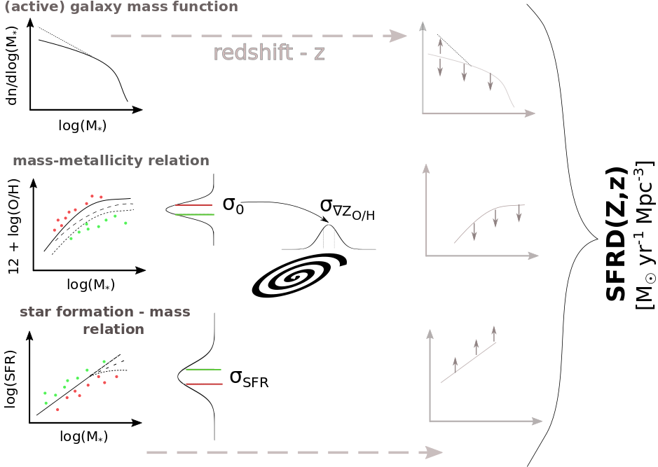
Figure 1: Schematic representation of our method. The observed stellar mass function of star forming galaxies gives the number density of objects of different masses. The mass $-$ metallicity relation allows us to assign metallicities to galaxies of different stellar masses. The star formation - mass relation allows us to specify the contribution of galaxies of different masses (metallicities) to the total star formation rate density at a certain redshift.
We vary the assumptions about those relations (low mass end slope of the GSMF, normalization and shape of the MZR, high mass end of the SFMR) to cover the range of possibilities present in the literature. We account for the intrinsic scatter present in the relations ($\sigma_{0}$, $\sigma_{SFR}$) and the observed anti-correlation between the SFR and metallicity. On top of that we introduce scatter in metallicity to account for the internal distribution of metallicities in the star forming gas within galaxies ($\sigma_{\nabla Z_{O/H}}$). All relations evolve with redshift.
Combining all relations we obtain the distribution of the cosmic star formation rate density over metallicities and redshifts SFRD(Z,z).

3.1 Galaxy stellar mass function

We use the published best-fit parameters to the Schechter (or double Schechter) function describing GSMF of star forming galaxies in different redshift bins at z$\lesssim$6. The studies used in the analysis are listed in Table 1. The last column of Table 1 gives the limits of the redshift bins in which the GSMF was estimated in each of those studies. We choose several values of redshift $z_{\rm avg}$ that overlap with the redshift bins in at least three of those studies . Those values are listed in the first column of Table 1.
To obtain the number density of star forming galaxies of a certain mass and at a certain redshift we:
(i) calculate the number density for that mass at $z_{\rm avg}$ redshifts as the average from the number densities calculated using the Schechter function fits referenced in Tab. 1
(ii) interpolate between the values found at different redshifts $z_{\rm avg}$
We treat the low and high mass part of the GSMF separately, calculating the number density of galaxies using the full Schechter fits as described above at $M_{\ast}>M_{\rm GSMF}$ and assuming that at lower masses the GSMF of star forming galaxies is described as a single power law with slope $\alpha_{\rm fix}$. We allow for two variations:

• $\alpha_{\rm fix}$=$-$1.45 at all redshifts

• $\alpha_{\rm fix}$=$\alpha_{\rm fix}(z)$ steepening with redshift according to the linear fit shown in Fig. 2 up to z=8 and fix $\alpha_{\rm fix}$=$-$2.14 at z$>$8 .

We assume that the mass separating the low and high mass part of the GSMF increases with redshift as log$\left(M_{\rm GSMF}/{\rm~{}M}_{\odot}\right)=7.8+0.4z$ up to $z$=5 and equals log$\left(M_{\rm GSMF}/{\rm~{}M}_{\odot}\right)$=9.8 at higher redshifts.
At $z<$0.05 we use the estimate obtained for $z$=0.05. To our knowledge there are no measurements of GSMF for the star forming population of galaxies at $z>$6. To extend our analysis to higher redshifts and constrain the GSMF evolution, we include the recent results obtained for the total sample of galaxies at $z\sim$7, $z\sim$8 and z$\sim$9 (Duncan et al., 2014; Grazian et al., 2015; Song et al., 2016; Bhatawdekar et al., 2019). This is justified as at such high redshifts the fraction of passive galaxies is expected to be very low (e.g. Muzzin et al., 2013; Henriques et al., 2015; Davidzon et al., 2017). At $z>$9 we assume that the normalization of the GSMF continues to mildly decrease at the rate found between z=8 and z=9. The resulting GSMF is shown in Fig. 3.

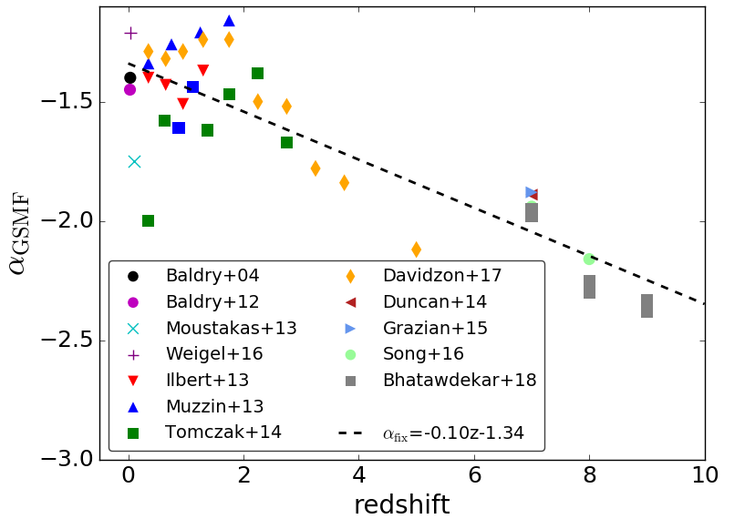
Figure 2: Low mass end slope ($\alpha_{\rm GSMF}$) values at different redshifts resulting from best (double) Schechter function fits to the galaxy stellar mass function of star forming galaxies ($z<6$) or GSMF of all galaxies ($z>$6) as found by different authors (see Tab. 1; the fixed $\alpha_{\rm GSMF}$ cases from Ilbert et al. (2013) and Muzzin et al. (2013) were excluded from the fit). The dashed line shows the linear fit used to describe the evolution of $\alpha_{\rm fix}(z)$ in those variations of our model in which we allow this slope to vary with redshift.

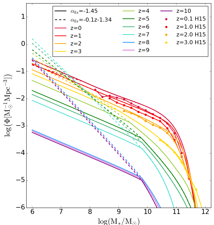
Figure 3: Galaxy stellar mass function of star forming galaxies used in our model, shown at different redshifts $z$. The solid lines show GSMF with the low mass end slope fixed to $\alpha_{\rm fix}$=$-$1.45, while the dashed lines show the case when the slope is allowed to evolve (steepen) with redshift. The observation-based GSMF of blue galaxies used by Henriques et al. (2015) to constrain their semi-analytic model is shown with the dot-connected lines at z=0.1, 1, 2 and 3 for comparison.

Table 1: The first column gives the redshift at which we average over the relations from studies listed in the second column in our model. The third column gives the IMF used in each study. The fourth column provides the slope of the low mass end of the star forming GSMF as fitted by the authors and the last one ($z_{bin}$) provides the redshift range of galaxies used by the authors to construct a GSMF of active galaxies. At $z$=0.95 we combine two redshift bins from Tomczak et al. (2014) and at $z$=3.5 two redshift bins from Davidzon et al. (2017), since those redshifts fall at the edge of their bins.
^a: using parameters fitted by Tomczak et al. (2014)
^b: the steeper slope from the fit to a double Schechter function
^c: the value was fixed during the fitting procedure
^d: GSMF describing the ‘total‘ sample of galaxies
^e: fits in parentheses include galaxies flagged by Bhatawdekar et al. (2019) as ‘point sources‘

z avg.	reference	IMF	$\alpha_{\rm GSMF}$	zbin
0.05	Baldry et al. (2004)	K01	$-$1.4b	0.01$-$0.08
	Baldry et al. (2012)	Ch03	$-$1.45	0.02$-$0.06
	Moustakas et al. (2013)a	Ch03	$-$1.75b	0.01$-$0.2
	Weigel et al. (2016)	K01	$-$1.21	0.02$-$0.06
0.35	Ilbert et al. (2013)	Ch03	$-$1.4b	0.2$-$0.5
	Muzzin et al. (2013)	K01	$-$1.34	0.2$-$0.5
	Tomczak et al. (2014)	Ch03	$-$2b	0.2$-$0.5
	Davidzon et al. (2017)	Ch03	$-$1.29b	0.2$-$0.5
0.65	Ilbert et al. (2013)	Ch03	$-$1.43b	0.5$-$0.8
	Muzzin et al. (2013)	K01	$-$1.26	0.5$-$1
	Tomczak et al. (2014)	Ch03	$-$1.58b	0.5$-$0.75
	Davidzon et al. (2017)	Ch03	$-$1.32b	0.5$-$0.8
0.95	Ilbert et al. (2013)	Ch03	$-$1.51b	0.8$-$1.1
	Tomczak et al. (2014)	Ch03	$-$1.61b	0.75$-$1
	Tomczak et al. (2014)	Ch03	$-$1.44b	1$-$1.25
	Davidzon et al. (2017)	Ch03	$-$1.29b	0.8$-$1.1
1.3	Ilbert et al. (2013)	Ch03	$-$1.37b	1.1$-$1.5
	Muzzin et al. (2013)	K01	$-$1.21	1$-$1.5
	Tomczak et al. (2014)	Ch03	$-$1.62b	1.25$-$1.5
	Davidzon et al. (2017)	Ch03	$-$1.24b	1.1$-$1.5
1.75	Ilbert et al. (2013)	Ch03	$-$1.6b,c	1.5$-$2
	Muzzin et al. (2013)	K01	$-$1.16	1.5$-$2
	Tomczak et al. (2014)	Ch03	$-$1.47b	1.5$-$2
	Davidzon et al. (2017)	Ch03	$-$1.24b	1.5$-$2
2.25	Ilbert et al. (2013)	Ch03	$-$1.6b,c	2$-$2.5
	Muzzin et al. (2013)	K01	$-$1.3c	2$-$2.5
	Tomczak et al. (2014)	Ch03	$-$1.38b	2$-$2.5
	Davidzon et al. (2017)	Ch03	$-$1.5b	2$-$2.5
2.75	Ilbert et al. (2013)	Ch03	$-$1.6b,c	2.5$-$3
	Muzzin et al. (2013)	K01	$-$1.3c	2.5$-$3
	Tomczak et al. (2014)	Ch03	$-$1.67b	2.5$-$3
	Davidzon et al. (2017)	Ch03	$-$1.52b	2.5$-$3
3.5	Ilbert et al. (2013)	Ch03	$-$1.6b,c	3$-$4
	Muzzin et al. (2013)	K01	$-$1.3c	3$-$4
	Davidzon et al. (2017)	Ch03	$-$1.78	3$-$3.5
	Davidzon et al. (2017)	Ch03	$-$1.84	3.5$-$4
5	Davidzon et al. (2017)	Ch03	$-$2.12	4$-$6
7	Duncan et al. (2014)d	Ch03	$-$1.89	6.5$-$7.5
	Grazian et al. (2015)d	Sal	$-$1.88	6.5$-$7.5
	Song et al. (2016)d	Sal	$-$1.94	6.5$-$7.5
	Bhatawdekar et al. (2019)d,e	Ch03	$-$1.98 ($-$1.95)	6.5$-$7.5
8	Song et al. (2016)d	Sal	$-$2.16	7.5$-$8.5
	Bhatawdekar et al. (2019)d,e	Ch03	$-$2.3 ($-$2.25)	7.5$-$8.5
9	Bhatawdekar et al. (2019)d,e	Ch03	$-$2.38 ($-$2.33)	8.5$-$9.5

3.2 Mass-(gas) metallicity relation

We start from the mass metallicity relation fitted by Maiolino et al. (2008) (in 3 redshift bins z$\sim$ 0.07, 0.7 and 2.2) and refined by Mannucci et al. (2009) (at z$\sim$3.5) We use a different parametrization of the MZR than in those two studies, given by eq. 3 and proposed by Moustakas et al. (2011).

$$\rm 12+log[O/H]=Z_{O/H\ asym}-log\left[1+\left(\frac{M_{\ast}}{M_{TO}}\right)^{-\gamma}\right]$$ (3)

This parametrization allows to avoid an artificial turn-off at the high mass part of the relation. The parameters are: $\gamma$ describing the low–mass end slope, $M_{\rm TO}$ – the mass at which the relation begins to turn/flatten and $Z_{O/H\ asym}$ – the asymptotic metallicity of the high-mass end. The relation given by Mannucci et al. (2009) was refitted in each of the redshift bins using this parametrization. We refer to this form of MZR as $M09$ throughout the paper. The gas metallicities in Mannucci et al. (2009) at 12+log[O/H]$>$8.35 dex were obtained with the Kewley & Dopita (2002) strong line calibration. We translate the base $M09$ relation at each redshift to three other calibrations (Tremonti et al. (2004) – $T04$, Kobulnicky & Kewley (2004) – $KK04$ and Pettini & Pagel (2004) O3N2 – $PP04$) applying the conversion method described in Kewley & Ellison (2008) at the high metallicity part (12+log[O/H]$>$8.35 dex) and fit the relation given by eq. 3 to the converted MZRs.

The fitted parameters are summarized in Table 2 .
We interpolate between the redshift bins to obtain the MZR at $0\leq\rm z\leq 3.5$ for each calibration. We assume that at higher redshifts the relation evolves in a mass independent fashion, i.e. only the normalization decreases. The rate of decrease in normalization (dZ_O/H/dz) at z$>$3.5 is assumed to be the same as the decrease in metallicity at $\rm M_{\ast}=10^{11}{\rm~{}M}_{\odot}$ between the two highest redshift bins (z=2.2 and z=3.5). Hence, for a given calibration the MZR at z$>$3.5 is given by:

$$\rm\left(12+log[O/H]\right)_{z>3.5}=\left(12+log[O/H]\right)_{z=3.5}+dZ_{O/H}/dz\times(z-3.5)$$ (4)

For a galaxy with mass $M_{*}$ at redshift $z$, we draw its average metallicity from the normal distribution centered at the metallicity taken from the MZR and with dispersion $\sigma_{0}$=0.1 dex at $M_{*}>10^{9.5}{\rm~{}M}_{\odot}$ and $\sigma_{0}$=–0.04 log(M${*}$/${\rm~{}M}_{\odot}$)+0.48 dex at higher masses. We add a normally distributed scatter around this value with $\sigma_{\nabla Z_{O/H}}$=0.14 dex to account for the distribution of metallicities at which the stars are forming within their host galaxies.

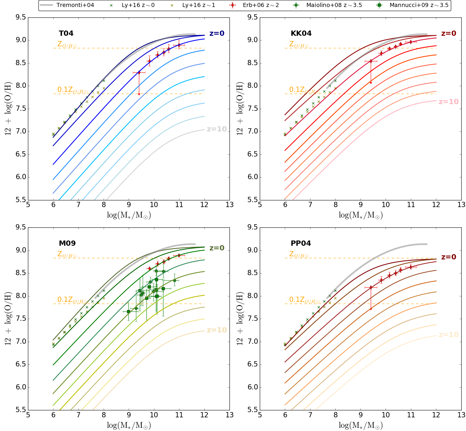
Figure 4: The four versions of the mass $-$ metallicity relation (MZR) used in this study. The relations were obtained using the results from Mannucci et al. (2009) (M09) and converting them to different metallicity calibrations (T04 $-$ Tremonti et al. (2004), KK04 $-$ Kobulnicky & Kewley (2004), PP04 $-$ Pettini & Pagel (2004) O3N2; see text). Each panel shows ten lines, corresponding to the MZR at different redshifts (z=0 $-$ top lines, z=10 $-$ bottom lines, $\Delta$z=1 spacing between the lines). The orange dashed horizontal lines mark the solar and 10% solar metallicity, assuming $Z_{O/H\odot}$=8.83 (Anders & Grevesse, 1989). For the reference, we plot the local MZR from Tremonti et al. (2004) at high stellar masses (thick gray line) and the MZR from Ly et al. (2016) at low stellar masses at z$\sim$0 and z$\sim$1 (dark and light green crosses respectively) in each panel. We also plot the data points from Erb et al. (2006) at z$\sim$2 (red points), converted to different metallicity calibrations where necessary. In the bottom left panel we additionally plot the data from Maiolino et al. (2008) and Mannucci et al. (2009) at z=3$-$4. We correct for different IMF where necessary.

Table 2: The parameters of the different versions of the mass $-$ metallicity relation used in this study. The first column gives the redshift, the second (fifth) column provides the low-mass end slope of the relation $\gamma$ , the third (sixth) column gives the logarithm of the turnover mass log$\left(\rm M_{TO}\right)$ and the fourth (seventh) column the asymptotic metallicity of the high mass end of the relation Z${}_{O/H\ asym}$ (see eq. 3). dZ_O/H/dz gives the rate of evolution of the MZR normalization at redshifts $>3.5$ (see eq. 4).

z	$\gamma$	log$\left(\rm M_{TO}\right)$	ZO/Hasym	$\gamma$	log$\left(\rm M_{TO}\right)$	ZO/Hasym
	T04; dZO/H/dz=$-$0.29 dex			M09; dZO/H/dz=$-$0.26 dex
0	0.66	9.39	9.12	0.63	9.25	9.08
0.7	0.61	9.86	9.15	0.57	9.72	9.11
2.2	0.62	10.59	9.07	0.59	10.46	9.04
3.5	0.62	10.67	8.70	0.60	10.54	8.72
	KK04; dZO/H/dz=$-$0.20 dex			PP04; dZO/H/dz=$-$0.24 dex
0	0.57	9.03	9.12	0.60	9.19	8.81
0.7	0.51	9.49	9.14	0.53	9.67	8.85
2.2	0.53	10.26	9.09	0.51	10.54	8.81
3.5	0.56	10.32	8.83	0.51	10.54	8.52

3.3 Star formation - mass relation

Following Boogaard et al. (2018), we describe the low mass part of the SFMR as a single slope power law with $a$=0.83 (see eq. 2). This slope does not evolve with redshift. We explore three variations of the SFMR shape at high masses:

• no flattening - we use the relation given by Boogaard et al. (2018) in the entire mass range (extrapolating beyond the mass range 7<log(M_∗)<10.5 covered in their study when necessary)

• moderate flattening - we use the relation given by Boogaard et al. (2018) at low masses and modify the slope at M${}_{\ast}\geq 10^{9.7}{\rm~{}M}_{\odot}$ according to the results obtained by Speagle et al. (2014) for M${}_{\ast}\geq 10^{9.7}{\rm~{}M}_{\odot}$ and 0<z<6. In this variation the slope of the high mass part of the SFMR is less steep than that of the low mass part and evolves with redshift, becoming steeper with increasing $z$. At z>6 we extrapolate the high mass-end slope evolution with time found by these authors.

• sharp flattening - we use the relation given by Boogaard et al. (2018) at low masses and combine it with the relation obtained by Tomczak et al. (2016) , which leads to flattening in SFMR at stellar masses above a certain turnover mass M${}_{\ast}\geq\rm M_{TO;\ SFMR}$. In this case SFR is almost constant with increasing M_∗ at M${}_{\ast}\geq\rm M_{TO;\ SFMR}$, as opposed to the ‘moderate flattening‘ variation, in which the slope changes but the SFR is still increasing with increasing mass. Tomczak et al. (2016) concluded that $M_{TO;\ SFMR}$ increases with redshift in the redshift range 0.5<z<4 covered in their study. At z<0.5 (z>3.28 ) we fix $M_{TO;\ SFMR}$ to the value that results from the relation fitted by these authors at z=0.5 (z=3.28).

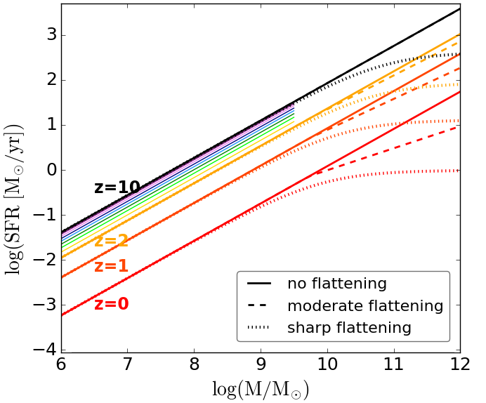
Figure 5: Star formation $-$ mass relation with three versions of the high-mass part shape: no flattening (solid), moderate flattening (Speagle et al., 2014) and sharp flattening (Tomczak et al., 2016) plotted at four example redshifts (z=0, z=1, z=2 and z=10, with the top lines corresponding to the highest redshift). Thin solid lines plotted at the low mass part of the relation at z$\geq$3 indicate the evolution of the normalization of SFMR at 10$>$z$\geq$3, with spacing of $\Delta z$=1 in redshift between them.

In all variations we keep the normalization given by Boogaard et al. (2018) (converted to Kroupa (2001) IMF) at low masses and z$\sim$0 and tie the high mass part of the relation to the low mass part accordingly. The normalization increases with redshift as $c\times\rm log(1+z)$ with $c$=2.8 at z$\leq$1.8 and $c$=1 at z$>$1.8 (see Fig. 5).
Similarly to the MZR, for any given stellar mass and redshift we assume that the SFR is normally distributed around the mean given by the SFMR with $\sigma_{\rm SFR}$=0.3 dex.

3.4 The model and its variations

Table 3 summarizes the default choice of parameters used in our calculations. The parameters that were varied are indicated in bold. We perform the calculations for 24 variations of the parameters of the model. Each variation is defined by the choice of MZR, SFMR flattening and $\alpha_{fix}$.

Table 3: The default choice of parameters used in our calculations. The parameters that were varied are emphasized in bold.

parameter	value/range	description
metallicity
$Z_{O/H}$	5.3 $-$ 9.7	12 + log(O/H) $-$ oxygen to hydrogen abundance ratio; binned, bin size = 0.022
$Z_{O/H\odot}$ ($Z_{\odot}$)	8.83 (0.017)	solar metallicity (Anders & Grevesse, 1989)
MZR	T04/M09/KK04/PP04	mass $-$ metallicity relation, varied: see Tab. 2 and Fig. 4
$\sigma_{0}$		scatter in the MZR (dispersion of the normal distribution):
	0.1 dex	at $\rm log(M_{*}/{\rm~{}M}_{\odot})>9.5$
	$-$0.04 $\rm log(M_{*}/{\rm~{}M}_{\odot})$+0.48 dex	at $\rm log(M_{*}/{\rm~{}M}_{\odot})\leq 9.5$
$\sigma_{\nabla Z_{O/H}}$	0.14 dex (but see appendix E.1)	dispersion of the normal distribution, $Z_{O/H}$ distribution within galaxies
star formation $-$ mass relation
SFMR flattening	none/moderate/sharp	the high mass end slope of the star formation $-$ mass relation; varied: see Fig. 5
$a$	0.83	slope of the SFMR at low masses (Boogaard et al., 2018)
$c$		redshift evolution coefficient of the SFMR (Sec. 3.3)
	2.8	$z<1.8$
	1	$z\geq$1.8
$\sigma_{SFR}$	0.3 dex	scatter in the SFMR (dispersion of the normal distribution)
galaxy stellar masses
log($M_{*}/{\rm~{}M}_{\odot}$)	6$-$12	logarithm of stellar mass of galaxies
Ngal	$10^{4}$	number of bins in stellar mass (equally spaced in logarithm)
Nsampl	50	number of galaxies sampled within each mass bin
$\boldsymbol{\alpha_{fix}}$	$-$1.45 or $-$0.1$\times\ z-$1.34	low mass end slope of the GSMF; varied (see Fig. 3 and Fig. 2)
other
IMF	K01; 0.1 $-$ 100 ${\rm~{}M}_{\odot}$	initial mass function (Kroupa, 2001)
$t$	464.4 $-$ 13465.7 Myr	time (age of the Universe), step size $\Delta t$= 100 Myr (if $\Delta z<$0.2) or calculated from $\Delta z$
$z$	0 $-$ 10	redshift, step size $\Delta z$=min( calculated from $\Delta$t or 0.2)

4 Results

One of the goals of this study is to find the observation-based distribution of the cosmic star formation rate density at different metallicities and redshift SFRD(Z,z). Given the currently unresolved observational issues, especially the unknown source of the differences between the metallicities measured using different calibrations and the shape of the high mass part of the SFMR (see sec 2), there is no simple, single answer to the question about the shape of the SFRD(Z,z). Hence, instead of indicating one ‘best‘ SFRD(Z,z) we first choose an example ‘moderate‘ variation of our model to discuss the general characteristics of the resulting distribution. We then discuss the differences between the variations allowed by the current observations and focus on the extreme cases that lead to the highest fraction of low/high metallicity star formation, which delineate the uncertainty of our result.

4.1 The distribution of the cosmic star formation rate at different metallicities and redshift: general picture

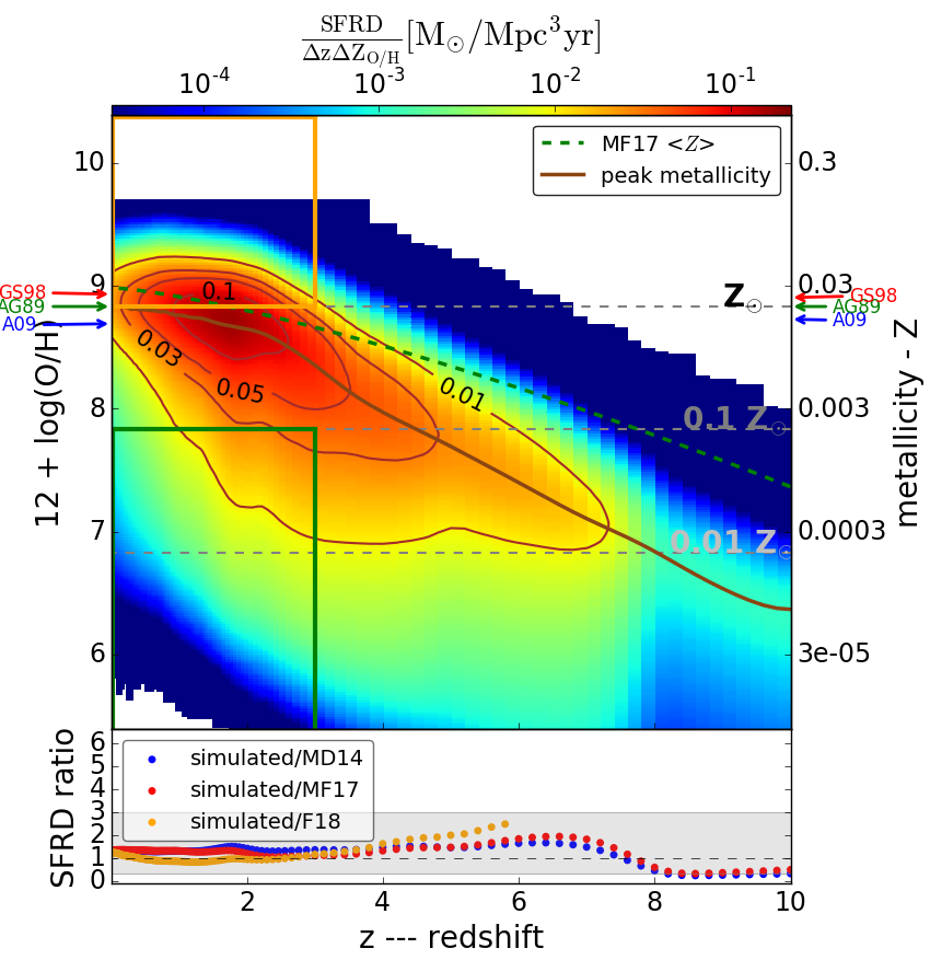
Figure 6: Upper panel: distribution of the star formation rate density (SFRD) at different metallicities and redshift ($z$) for the model described in Sec. 4.1. The right scale assumes solar metallicity from Anders & Grevesse (1989) (green arrows). The $Z_{O/H\odot}$ and ${\rm~{}Z}_{\odot}$ estimates by Asplund et al. (2009) (Grevesse & Sauval 1998) are shown with blue (red) arrows for the reference. The colour indicates the amount of SFRD at each metallicity and $z$, with most of the star formation happening in the red region of the $z$ $-$ metallicity space. The brown line indicates $Z$ corresponding to the peak of the distribution at each $z$ and several contours of the constant SFRD. The dashed green line shows the mass-averaged mean $Z$ estimate from Madau & Fragos (2017) (see Sec. 6.3). In Sec. 4.2.2 we compare the model variations by comparing the fraction of stellar mass formed above $Z_{O/H\odot}$ and below 10% $Z_{O/H\odot}$ since $z$=3 (i.e. within the orange and green rectangles). Bottom panel: the ratio of the total SFRD($z$) (summed over metallicities) calculated in our model and inferred from observations (blue $-$ MD14; Madau & Dickinson (2014), red $-$ MF17; Madau & Fragos (2017), orange $-$ F18; Fermi-LAT Collaboration et al. (2018)). A factor of three deviation from unity is indicated by the gray area.

Figure 6 shows distribution of the star formation rate density at different metallicities and redshifts calculated assuming a moderate flattening at the high mass end of SFMR, M09 mass metallicity relation and fixed low mass end slope of the galaxy stellar mass function $\alpha_{fix}$=$-$1.45. We use this variation as an example to point out the main characteristics of the SFRD(Z,z) that are common to all model variations:

• At low $z$ the star formation is concentrated at relatively high metallicities; the location of the peak (thick brown line in Fig. 6) depends primarily on the MZR

• The metallicity at which SFRD(z) peaks decreases towards higher $z$, reflecting the evolution of the MZR. The decrease rate increases around the redshift $\gtrsim$2 and depends on the MZR.

• The global peak of the distribution is reached at $z\sim$1.8, coinciding with the peak of the star formation history of the Universe, and at $Z$ that depends on the model variation (primarily MZR)

• The distribution is asymmetric with respect to the peak metallicity, showing the extended tail at low $Z$ (see also Fig. 14). The contribution from the tail to the total SFRD(z) at high $z$ is noticeably higher in the variations with $\alpha_{fix}$=$\alpha_{fix}(z)$ (see Fig. 7).

The bottom panel of Figure 6 shows the redshift evolution of the ratio of the total SFRD(z) in our simulations to the SFRD from observational studies by Madau & Dickinson (2014), Madau & Fragos (2017) an Fermi-LAT Collaboration et al. (2018). We note that the only way the total observed SFRD was used in our model is to set the redshift at which we change the rate of redshift evolution of the SFMR normalization . Thus, this comparison is still a valid test for our model. The total simulated SFRD shows a remarkable agreement with observations up to very high redshifts, staying within a factor of 2$-$3 from the observed SFRD up to $z\sim$8 for all variations that assume $\alpha_{fix}$=$-$1.45 (but not for the cases with $\alpha_{fix}$=$\alpha_{fix}(z)$, see Sec. 4.1.1).

Note that the model variations that differ in the assumptions about the SFMR and/or GSMF lead to different total SFRD(z) (which sets the normalization of the SFRD(Z,z)). In general, SFRD increases up to $z\sim 1.8$, decreases towards higher $z$ and declines sharply around $z\sim 8$. This evolution is a result of the interplay between the evolving SFMR and GSMF, mostly their normalizations. The shape of both relations also changes with redshift, but it has a secondary effect on the evolution of the total SFRD (except for the cases with $\alpha_{fix}$=$\alpha_{fix}(z)$ at $z\gtrsim 4$). At $z\sim$8 the normalization of the GSMF decreases abruptly (see fig. 3), which results in an apparent jump in the normalization in Figure 6.

4.1.1 The variations with $\alpha_{fix}$=$\alpha_{fix}(z)$

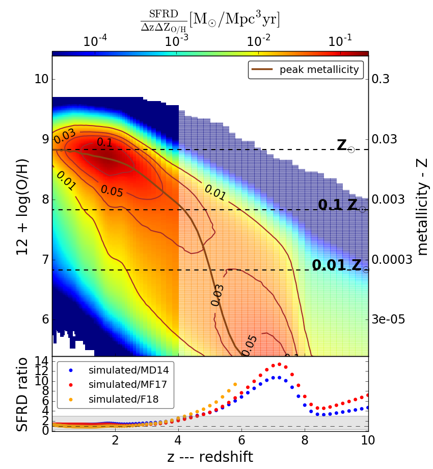
Figure 7: Same as Figure 6, but calculated for the variation in which the low mass end slope of the GSMF evolves with redshift $\alpha_{fix}$=$\alpha_{fix}(z)$. Note that at high redshifts z$\gtrsim$4 (shaded area) the SFRD(z) is significantly higher than estimated from observations (bottom panel; see Sec. 4.1.1 for the details). This is true for all variations with $\alpha_{fix}$=$\alpha_{fix}(z)$. Those variations were excluded from the analysis at z$\gtrsim$4. For further description see the caption of Fig. 6.

When the low mass end slope of the GSMF is allowed to evolve (steepen) with redshift according to the fit shown in Fig. 2, the resulting SFRD(Z,z) distribution starts to deviate significantly from the picture shown in Fig. 6 at $z\gtrsim 4$. The SFRD(Z,z) distribution calculated assuming the same relations as in the case shown in Fig. 6, but with evolving $\alpha_{fix}$=$\alpha_{fix}(z)$ is shown in Figure 7 (the other model variations with $\alpha_{fix}$=$\alpha_{fix}(z)$ show the same qualitative behavior).
The normalization of the SFMR continuously increases with redshift, which means that galaxies at all masses produce stars at higher rates. At the same time, the normalization of the GSMF decreases and the cut off mass shifts to smaller values, both reducing the number density of the most massive galaxies (with the highest SFR and $Z$ at a certain redshift). $\alpha_{fix}$ decreases (the slope steepens), increasing the number of low mass galaxies and the shape of the GSMF evolves almost into a single power-law (see fig. 3). This, together with continuously increasing SFR(M_∗) produces a plateau in the total SFRD(z) in our simulations at z$\sim$4-7 (see e.g. fig. 10, showing the core collapse supernovae rate, which is proportional to the total SFRD(z)). The low mass galaxies begin to dominate the total star formation budget and the peak of the SFRD(Z,z) shifts to very low metallicities (below 1% ${\rm~{}Z}_{\odot}$ at $z\sim$5).
Such plateau in SFRD(z) at z$\sim$4$-$7 is not found within the current observational studies (predicting a continuous decrease in the total SFRD(z) at these high redshifts) and hence the bottom panel of Fig. 7 shows that our simulations start to significantly overpredict the total SFRD at z$\sim$6.
Taking this into account, we consider the high redshift ($z\gtrsim 4$) predictions of the model variations with $\alpha_{fix}$=$\alpha_{fix}(z)$ unreliable and exclude them from further analysis, while still taking them into consideration at lower redshifts. We return to that discrepancy at high redshifts in Sec. 6.1.

4.2 The extreme cases

The main purpose of this study is to identify the model variations that lead to the most extreme pictures of the SFRD(Z,z) and hence delineate its uncertainty.
Different assumptions about the amount of star formation occurring at low metallicities can lead to significant differences e.g. in the obtained properties of the progenitors of merging double black holes and long gamma ray bursts and the inferred rates of transients connected to those objects. Keeping in mind the importance of metallicity, we interpret extremes as variations that lead to the smallest and the highest fraction of stellar mass forming at low/high metallicity.
The main differences in the SFRD(Z,z) distributions obtained for different model variations are the following:

• The location of the peak metallicity and the slope of the curve indicating the peak metallicity at each redshift

• The extent of the low metallicity tail and its contribution to the total SFRD(z)

• Normalization of the distribution / total SFRD(z)

Focusing on the fraction of stellar mass formed at low and high metallicity means that we set aside the differences in normalizations (but see Sec. 4.3).
The location of the peak metallicity and the rate of its decrease with $z$ are set primarily by the choice of the MZR – the relation with high, slowly decreasing normalization will maximize the fraction of stellar mass forming at high metallicity. The slope of the MZR affects the low metallicity tail of the SFRD(Z,z) - the flatter the relation, the smaller the difference in metallicity of stars forming in galaxies of different masses and the the low-Z tail is reduced.
Furthermore, the choice of the SFMR regulates the contribution of the most massive galaxies (forming stars at high metallicities) to the total SFRD(z). Hence, the SFMR with no flattening maximizes the high metallicity star formation, and the reverse is true for the SFMR with sharp flattening
Finally, the low mass end slope of the GSMF regulates the contribution of galaxies with the lowest masses. The steeper the slope, the more low mass galaxies (and hence more stars forming in the low metallicity tail of the distribution).
Thus, one can expect the extreme variations to be represented by the combination of $KK04$ MZR, SFMR with no flattening and $\alpha_{fix}$=$-$1.45 (the high metallicity extreme) and $PP04$ MZR, SFMR with sharp flattening (the low metallicity extreme).

4.2.1 SFRD(Z,z) for the extreme cases

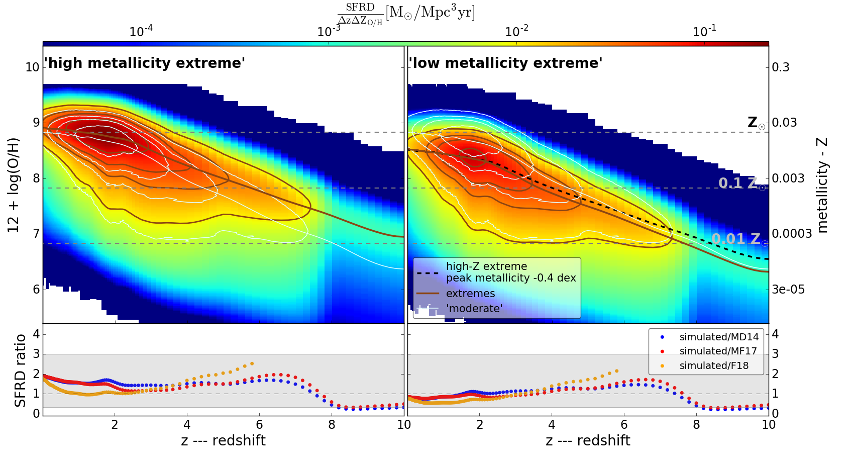
Figure 8: Upper panels: distribution of the star formation rate density (SFRD) at different metallicities and redshift ($z$). Left – the model variation that leads to the highest fraction of mass formed at high metallicities, right – the model variation that leads to the highest fraction of mass formed at low metallicities. Difference between the two extremes depicts the uncertainty of the SFRD(Z,z) based on the observational properties of star forming galaxies.
The thick brown line indicates the metallicity corresponding to the peak of the SFRD(z) and the contours of constant SFRD (with the same levels as in Fig. 6). We overplot the contours calculated for the moderate variation discussed in Sec. 4.1 and plotted in Fig. 6 (thin white line). The thick dashed black line in the right panel shows the peak metallicity from the left panel, downshifted by 0.4 dex to match the metallicities of both extremes at $z\sim 1.8$. Bottom panels: the ratio of the total SFRD(z) calculated in the two variations of our model and as inferred from observations. For further description see the caption of Fig. 6

The distributions of the star formation rate density across metallicities and redshifts for the extreme cases identified in Sec. 4.2 are shown in Figure 8. The difference between the two panels visually demonstrates the uncertainty of the SFRD(Z,z) due to unresolved questions in the determination of various characteristics of galaxies (absolute metallicity scale, high mass end of the SFMR and low mass end of the GSMF).

To facilitate the comparison, we overplot the constant SFRD contours and the line showing peak metallicity at each redshift for the moderate variation shown in Fig. 6. The left panel of Figure 8 shows the high metallicity extreme. The low metallicity extreme is shown in the right panel.
As shown in the right panel in Fig. 8, except for the $\sim$0.4 dex offset, the redshift evolution of the peak metallicity for both extremes is very similar. This stems from the fact that MZRs obtained for different metallicity calibrations have similar shape (i.e. are relatively flat) in the high mass part that contributes the most to the total star formation. At higher redshifts $z\gtrsim 2$ the peak metallicity lines for both cases start to deviate due to different rates at which the MZR normalization decreases for both relations (the PP04 MZR normalization decreases at a higher rate than KK04; see Table 2). The peak metallicity reaches our conventional low metallicity limit of 0.1${\rm~{}Z}_{\odot}$ at z=5.8 and z=3.6 for the high and low metallicity extreme respectively and never drops below 0.01${\rm~{}Z}_{\odot}$ in the former case.
Note that the low metallicity extreme has a lower SFRD(z) and leads to smaller total stellar mass than the moderate variation and the high metallicity extreme (see Sec. 4.3).

4.2.2 Quantifying the differences between the variations

In this section we aim to quantify the differences between the model variations discussed above, in particular to find the maximum difference between the fraction of stellar mass formed at low and high metallicity across the considered variations.
For presentation purposes we adopt the conventional limits of $Z<$0.1${\rm~{}Z}_{\odot}$ and $Z>{\rm~{}Z}_{\odot}$ to define the low and high metallicity respectively (assuming solar abundances according to Anders & Grevesse, 1989). We note that this particular choice does not affect our conclusions.
In our analysis we focus on three redshifts ranges: $z<0.5$ to which we refer as the ‘local Universe‘ and which can be probed with the current network of ground-based gravitational wave detectors, $z<3$ up to which redshift our model is still reasonably well backed up by the current observational results and which captures the great majority of the star formation history of the Universe and $z<10$ where we extend our calculations beyond redshifts directly probed in observational studies relying on extrapolations. Those redshifts correspond to $\sim$12.8 Gyr, $\sim$2.1 Gyr and $\sim$0.46 Gyr respectively in terms of the age of the Universe. The example distribution of stellar mass formed since $z$=3 across metallicities is shown in appendix C.1.

Figure 9 shows the fraction of stellar mass formed at low metallicities versus that formed at high metallicities since $z$=0.5, 3 and 10 for our model variations. It can be seen that, as expected, variations leading to the highest fraction of mass formed at low metallicities at the same time produce the lowest fraction of high metallicity stars (and vice versa) at all redshifts and the extreme cases introduced earlier in Sec. 4.2 can be easily identified (low-Z extreme $-$ brown circles; high-Z extreme $-$ red squares). Note that when the stellar mass formed since $z>1.5$ is considered, the fraction of stellar mass formed at low-Z is additionally increased if the low mass end slope of the GSMF is allowed to steepen with $z$ (compare brown circles with and without edge). The impact of different assumptions on the low-$Z$ mass fraction is further discussed in appendix C.2.

The difference between the fraction of the mass formed at low and high metallicity produced in the two extremes is quite significant. Those values (summarized in Table 4) range between $\sim$3%$-$15% and $\sim$4%$-$55% at $z\leq$0.5, $\sim$9%$-$27% and $\sim$1%$-$27% at $z\leq$3 and $\sim$17%$-$43% and $\sim$0.7%$-$19% at $z\leq$10 for the low and high metallicity fractions respectively.
For the example variation shown in Fig. 6 (with M09 MZR, moderate SFMR flattening and non-evolving $\alpha_{fix}$) the corresponding values are 6% and 38% at $z\leq$0.5, 15% and 15% at $z\leq$3, and 29% and 11% at $z\leq$10. We note that it does not fall exactly in between the low and high metallicity star formation extremes, but produces a higher fraction of mass at high metallicities with respect to a simple average. While it represents the ‘most moderate‘ case considered in this study (and hence we refer to it as the moderate variation), the results obtained for the T04 MZR (for the same assumptions about the SFMR and GSMF) are comparable. This highlights the question of degeneracies involved in our calculations. Similar results could be obtained using another MZR (resulting from a different metallicity calibration), or by combining it with different assumptions about the SFMR and/or GSMF that fall between the extreme cases considered in our work.

In nearly all cases, the summed fraction of stellar mass produced at low and high metallicity is smaller than 0.5. This means that in those variations most of the stellar mass forms outside the assumed low and high metallicity regimes (i.e. between 0.1${\rm~{}Z}_{\odot}$ and ${\rm~{}Z}_{\odot}$ or, equivalently, between $Z_{O/H}$=7.83 and $Z_{O/H}$=8.83) . We look in more detail at the location of the peak of the distribution - i.e. metallicity at which most of the stellar mass formed in different redshift ranges and model variations in appendix C.1.

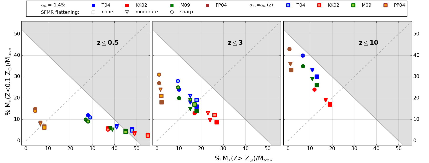
Figure 9: The fraction of mass formed in stars at low ($<0.1{\rm~{}Z}_{\odot}$) vs at high ($>{\rm~{}Z}_{\odot}$) metallicities since redshift z=0.5 (left), z=3 (middle) and z=10 (right) for different model variations. Different symbols distinguish the assumptions about the high mass part of the SFMR while the colours distinguish the assumptions about the MZR and low mass end slope of the GSMF. We exclude the variations with $\alpha_{fix}(z)$ at z$\gtrsim$4 (see Sec. 4.1.1). The results shown in Fig. 6 (7) correspond to the variation indicated with the dark (light) green triangle. The extreme cases discussed in Sec. 4.2.1 are indicated with the dark red square and brown/orange circle. The dashed diagonal line corresponds to equal percent of $M_{*}$ formed at low and high $Z$. Almost all points fall outside the gray shaded area, which means that more than 50% of $M_{*}$ formed at metallicities between 0.1 ${\rm~{}Z}_{\odot}$ and ${\rm~{}Z}_{\odot}$.

4.3 Total stellar mass vs the mass fraction

Table 4: Total stellar mass (column 3) formed since redshift $z_{i}$ (column 1) in different versions of the model and fraction of that mass formed at low (column 4) and high (column 5) metallicity. The second column specifies the shape of the high mass end of the SFMR. The lowest (highest) value given in the column 4 (5) corresponds to the KK04 MZR. The highest (lowest) value given in the column 4 (5) corresponds to the PP04 MZR. $z_{i}$=10 was not included for the $\alpha_{fix}$=$\alpha_{fix}(z)$ due to the reasons discussed in Sec. 4.1.1.

zi	SFMR flattening	$\frac{M_{tot\ast}(z\leq z_{i})}{{\rm~{}M}_{\odot}}$	$\frac{\rm M_{\ast}(Z<0.1{\rm~{}Z}_{\odot})}{\rm M_{tot\ast}}$	$\frac{\rm M_{\ast}(Z>{\rm~{}Z}_{\odot})}{\rm M_{tot\ast}}$
$\alpha_{fix}$=$-$1.45
0.5		5.1$\times 10^{18}$	0.03-0.07	0.08-0.55
3	none	5.4$\times 10^{20}$	0.09-0.18	0.02-0.27
10		7.6$\times 10^{20}$	0.17-0.33	0.01-0.19
0.5		2.3$\times 10^{18}$	0.06-0.15	0.04-0.37
3	sharp	3.6$\times 10^{20}$	0.13-0.27	0.01-0.17
10		5.4$\times 10^{20}$	0.24-0.43	0.01-0.12
0.5		4$\times 10^{18}$	0.04-0.09	0.07-0.49
3	moderate	4.8$\times 10^{20}$	0.10-0.21	0.02-0.24
10		6.9$\times 10^{20}$	0.19-0.36	0.01-0.17
$\alpha_{fix}$=$\alpha_{fix}(z)$
0.5		5.1$\times 10^{18}$	0.02-0.06	0.08-0.55
3	none	5.6$\times 10^{20}$	0.12-0.21	0.02-0.26
0.5		2.3$\times 10^{18}$	0.05-0.14	0.04-0.37
3	sharp	3.8$\times 10^{20}$	0.17-0.31	0.01-0.17
0.5		3.9$\times 10^{18}$	0.03-0.08	0.06-0.49
3	moderate	4.9$\times 10^{20}$	0.13-0.24	0.02-0.23

The different variations do not only lead to different fractions of stellar mass formed at high and low metallicity, but also produce different total stellar mass (see Table 4). Variations with no flattening in the SFMR lead the highest total $M_{*}$ because they produce more stars in the high-mass galaxies (with high SFR and $Z$).
This effect reduces the difference in the total mass formed at low metallicity and increases the difference in terms of the total mass formed at high metallicity between the variations with different assumptions about the SFMR.
Using the values given in Table 4, we find that the total mass formed at low metallicity across the model variations differs by less than a factor of 3 and is relatively well constrained within our study.
The corresponding values of the mass formed at high metallicity span a much wider range and the differences between the model variations reach up to a factor of $\sim$40.

5 Application of the model: core collapse supernovae rates

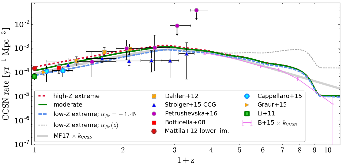
Figure 10: Core-collapse supernovae (CCSN) rate calculated using our model (short dashed red line $-$ high metallicity extreme; solid green line $-$ moderate; thick blue long dashed line $-$ low metallicity extreme; thin gray dashed line $-$ low metallicity extreme with $\alpha_{fix}$ evolving with redshift) compared with the observational estimates (Botticella et al., 2008; Li et al., 2011; Dahlen et al., 2012; Mattila et al., 2012; Cappellaro et al., 2015; Graur et al., 2015; Strolger et al., 2015; Petrushevska et al., 2016, see legend). In case of Strolger et al. (2015) we plot the CANDLES+CLASH+GOODS based estimate (Strolger+15 CCG) as given by the authors and include the ‘extinction limits‘ systematic uncertainty (see Tab. 3 and 4 therein). In case of the model results we assume that CCSN progenitors come from the initial mass range 8-25 ${\rm~{}M}_{\odot}$. For the reference, we also plot the SFRD(z) from Madau & Fragos (2017) (MF17, thick gray solid line) and the high redshift SFRD estimate by Bouwens et al. (2015) (B+15, magenta line; converted to our default Kroupa (2001) IMF) multiplied by the efficiency of formation of CCSN progenitors ($k_{CCSN}\sim 0.009\ {\rm~{}M}_{\odot}^{-1}$; assuming CCSN mass range 8$-$25 ${\rm~{}M}_{\odot}$ and Kroupa 2001 IMF).

Core-collapse supernovae (CCSN; i.e. Type II and Ib/c SNe) originate from short-lived massive stars and can serve as an independent tracer of the star formation (e.g. Madau & Dickinson, 2014). We can thus confront the predictions of our model with the volumetric CCSN rate estimates at different redshifts, assuming that the volumetric CCSN rate is proportional to the SFRD(z). However, one should keep in mind that there is a number of factors that make this comparison not straightforward and may cause deviations from the simple proportionality (see appendix D.1).
In Figure 10 we plot the observational CCSN rate estimates at different redshifts against the star formation rate density for the two extreme cases and the moderate variation of our model discussed in Sec. 4, multiplied by a constant factor $k_{CCSN}\sim 0.009\ {\rm~{}M}_{\odot}^{-1}$. This factor comes from a simple IMF-based scaling and corresponds to the efficiency of formation of CCSN progenitors assuming our default Kroupa (2001) IMF and CCSN forming form single stars with masses between 8$-$25 ${\rm~{}M}_{\odot}$ , which given the large scatter in the observations, provides a satisfying match to the data.

The knowledge of the distribution of the cosmic star formation over metallicities allows us to compare not only with the global volumetric CCSN rate discussed above, but also to perform a more detailed comparison with the CCSN rates measured as a function of metallicity. We calculate the specific CCSN rate as a function of metallicity (number of CCSN in a certain metallicity bin divided by the stellar mass in galaxies in that metallicity bin) and use the mass range for the CCSN progenitors estimated based on the comparison with the volumetric rates to get the normalization. Those rates can be confronted with the specific CCSN rates based on the Lick Observatory Supernova Search (LOSS) sample from Graur et al. (2017) . Figure 11 shows the specific rates at z$\lesssim$0.02, which roughly corresponds to the redshift range relevant for the LOSS SN sample. We show the results for the model variations using the T04 MZR, as this was the metallicity calibration used in Graur et al. (2017).
The metallicity measurements used in Graur et al. (2017) are based on the SDSS observations and correspond to the central metallicity within the CCSN host galaxy. The central metallicity is typically higher than the metallicity at the CCSN location (due to radial metallicity gradients, see Sec. 2.3.3). It is also higher than the metallicity probed by the MZR, which gives the ‘averaged‘ global value (and corresponds roughly to the metallicity that would be measured at the distance of one effective radius r_e). Therefore, an offset in metallicity between the data and the results from our model can be expected. To be conservative in our comparison, we extend the horizontal errorbars of the data shown in Figure 11 by 0.24 dex towards lower metallicity, assuming that the great majority of the observed CCSN explosion site metallicities would be contained within that range (see appendix D.2). This wide range, together with the uncertain translation of the amount of star formation to the number of core collapse supernovae (which affects the location of the model curves on the vertical axis) precludes us from drawing any strong conclusions from that comparison. In general, we find a reasonably good agreement of our model with the data. However, we note that the dotted curve in Fig. 11 which corresponds to the model variation with the sharp flattening in the high mass end of the SFMR, falls slightly outside the extended uncertainty regions of the data points. Hence, the model variations with a sharp flattening in the SFMR may underestimate the amount high metallicity star formation in the local Universe.

We note that the slope of the high metallicity part of the relation plotted in Fig. 11 depends on the combination of the scatter present in the MZR ($\sigma_{0}$) and on the width of the distribution of metallicities at which the stars form within galaxies ($\sigma_{\nabla O/H}$; see appendix D.3). The slope cannot be directly compared with the data from Graur et al. (2017), as they only provide the central metallicities of CCSN host galaxies, but could potentially be probed with similar observations that provide metallicity measurements at SN location.

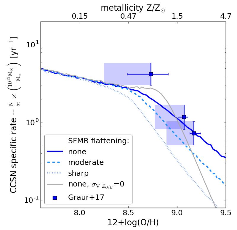
Figure 11: The specific CCSN rate as a function of metallicity for different model variations (SFMR with no flattening – thick solid line, moderate flattening – dashed line, sharp flattening – dotted line) and observations (Graur et al. (2017)¹⁸). The metallicity scale assumes the T04 calibration¹⁹. The thin solid line shows the case with no flattening and without taking into account the metallicity distribution within galaxies. The blue shading shows the additional uncertainty ($-$0.24 dex) due to the fact that the $Z_{O/H}$ in the observed sample was measured in the central region of the SN host galaxy and not at the SN location. Our model shows satisfying agreement with the data, although the variations with sharp flattening in SFMR may underestimate the local high-Z star formation.

6 Discussion

In this section we further comment on the reliability of our results at high redshifts and on the adopted extrapolations. We also discuss some of the simplifications present in our method. Finally, we place our results in the context of previous studies and perform a brief comparison with the predictions of cosmological simulations.

6.1 Reliability of our results at high redshifts

The current observational estimates of the GSMF used in our study reach to $z\sim 9$ and the rate of redshift evolution of the SFMR was also constrained at these high redshifts (e.g. Bhatawdekar et al., 2019). However, the shape and evolution of the gas-phase MZR is essentially unconstrained above z$\sim$3.5 with the current observations (see Sec. 2.3.1) and our results at higher redshifts need to be taken with a grain of salt.
The observational estimates of the total cosmic SFRD (reaching even up to $z\sim 10$ e.g. Bouwens et al., 2015) can serve as constraints to our model, allowing to validate the combined assumptions about the SFMR and GSMF. SFRD(z) recovered from our model shows a reasonable agreement with the observations up to z$\gtrsim$8 for all variations in which the low mass end slope of the GSMF for star forming galaxies does not evolve with redshift ($\alpha_{fix}=-1.45$).
However, there seems to be overall trend for $\alpha_{fix}$ to steepen with redshift (see Sec. 2.1 and Fig. 3). When we allow $\alpha_{fix}$ to evolve according to the fit presented in Fig. 3, the cosmic SFRD(z) starts to significantly deviate from the observational estimates around $z\gtrsim$4 (see Sec. 4.1.1). The cause of this discrepancy is not clear.
One of the assumptions which may be responsible for this problem is that the low-mass end slope of the SFMR ($a$=0.83) does not evolve with redshift. As discussed in Sec. 2.4.1, it is difficult to constrain the evolution of $a$ with the current observations. If the value of $a$ would increase with redshift, the amount of star formation occurring in low mass galaxies could be reduced and this would alleviate the tension with the cosmic SFRD. Such evolution has been reported by several authors (e.g. Whitaker et al., 2014; Pearson et al., 2018), while some other studies observe the reverse trend (e.g. Kurczynski et al., 2016; Bisigello et al., 2018). Another argument in favor of the steepening $a$ comes from the studies comparing the evolution of the stellar mass buildup resulting from the SFMR and as is observed from the evolution of the GSMF (e.g. Weinmann et al., 2011; Leja et al., 2015). The observationally inferred SFMR is known to lead to an overabundance of the low mass galaxies with respect to the GSMF even when the high merger rate (shifting some of the excess galaxies to higher masses) is assumed for those galaxies. Leja et al. (2015) show that $a\sim$1 at low masses (especially at the high redshift end of the redshift range considered in their study z$\lesssim$2 ) helps to improve the consistency (although does not entirely solve the problem).
The inconsistency found in our variations with $\alpha_{fix}$=$\alpha_{fix}(z)$ may also arise from the assumed extrapolations to low stellar masses. We extend the scaling relations and GSMF down to $M_{\ast}=10^{6}{\rm~{}M}_{\odot}$, which is much lower than the stellar mass that can be probed by any high-redshift survey. In principle, there is no guarantee that the slope of the GSMF and SFMR does not change at stellar masses below the range probed by the current observations or that such a turnover appears at high redshifts. In fact, recent studies by Bouwens et al. (2017) and Atek et al. (2018) investigating the galaxy luminosity function (LF) in the extremely faint regime with lensed galaxies find support for the presence of a flattening/turnover in the LF at $z\sim$6 and absolute UV luminosities $M_{UV}\gtrsim-15$ mag . The upper limit on the UV emissivity at z$\sim$5$-$6 found by Fermi-LAT Collaboration et al. (2018) also favors the presence of a turnover in the LF at $M_{UV}\gtrsim-14$ mag. However, the flattening/turnover at these low luminosities is not likely to solve the discrepancy observed in our model.
Finally, we note that systematic trends in the IMF (e.g. with metallicity/redshift), if present, could have a strong and non-straightforward effect on our results (see Sec. 2.6).

6.2 Comparison with the Illustris cosmological simulations

While the comparison with the predictions of cosmological simulations cannot settle the correctness of our results, it is certainly interesting to confront the two methods, especially in the regimes not covered by observations. Here we briefly compare our results with the predictions of the large-scale Illustris-1 cosmological hydrodynamical simulations (Vogelsberger et al., 2014) presented in Fig 1. in Bignone et al. (2017), leaving a more detailed comparison with the simulations for future studies. The comparison is shown in Fig. 12. The right panel reproduces Fig. 1 from Bignone et al. (2017) with additional curves corresponding to the results from our model. We show only three (out of six) lines presented in Fig. 1 in Bignone et al. (2017) to improve the readability of the plot. Those are the lines corresponding to the total SFRD (no cut in Bignone et al. 2017; green lines), the SFRD occurring below $Z$=0.0038 (0.3${\rm~{}Z}_{\odot}$ cut in Bignone et al. 2017 $-$ ${\rm~{}Z}_{\odot}=0.0127$ in their paper; brown lines) and the SFRD occurring below $Z$=0.0013 (0.1${\rm~{}Z}_{\odot}$ cut in Bignone et al. 2017; orange lines). None of the curves corresponds to super-solar metallicity (as Bignone et al. 2017 focus on long GRB host galaxies) and hence we cannot compare the distributions in that regime. The comparison reveals that the closest match between the Illustris-1 results and our model can be found for the low metallicity extreme variation (the ratio stays within a factor of 2.5 up to $z\sim$8). The ratio changes only slightly if a different SFMR flattening is used in combination with the PP04 MZR (e.g. no flattening in SFMR instead of the sharp flattening used in the low-Z extreme variation; compare solid and dashed lines in the middle panel on the left in Fig. 12). The best agreement is reached for the $Z$=0.0038 metallicity cut. The SFRD occurring below $Z$=0.0013 in this variation is underpredicted with respect to the Illustris-1 simulations at $z\lesssim$2 and overpredicted at $z\gtrsim$3, which suggests that the chemical evolution of the simulated universe is slower than in our case. In any case, at $z\sim$8 the SFRD from our model shows a steep decrease $-$ the consequence of the evolution of the GSMF $-$ not reflected in the results from simulations. The Illustris-1 simulations predict higher star formation rate density at $z\lesssim$2 than our model and also more low metallicity star formation up to $z\sim$5 and above z$\sim$8 for the moderate and high-Z extreme variations.
We note that the results of the comparison would likely change for the updated IllustrisTNG simulations (e.g. Pillepich et al., 2018; Torrey et al., 2019), as one of the primary differences with respect to Illustris-1 is connected to the mass-metallicity relation from the simulations (Torrey et al., 2019). Torrey et al. (2019) report the improved agreement with the observed MZR, e.g. the flattening of the relation at high masses, which was not reproduced in the previous version (Torrey et al., 2014) is now accounted for. Also, the slope of the simulated MZR has changed. The normalization of the MZR found in IllustrisTNG continuously decreases with redshift, with the average rate at $z>2$ of $\approx-0.064$ dex per $\Delta z$=1. We note that this rate is much lower than assumed in our model based on the observed evolution between $z$=2.2 and $z$=3.5 (see Sec. 2.3.1 and 3.2).

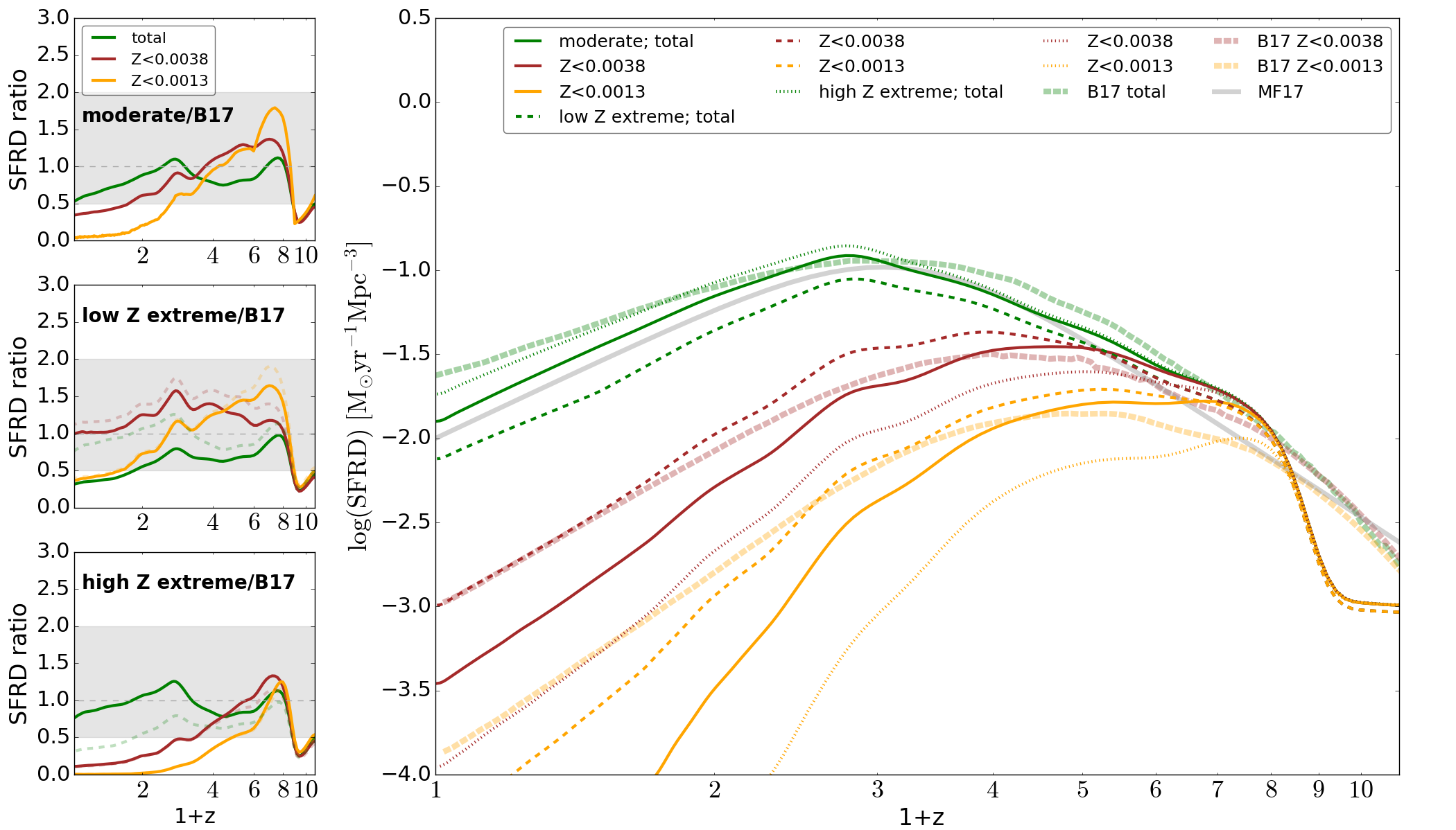
Figure 12: Comparison between the results from this study and the results from the Illustris-1 cosmological simulations shown in Bignone et al. (2017) (B17; see Fig. 1 therein). The right panel shows the cosmic star formation rate density; total (green lines) and below certain metallicity thresholds: Z$<$0.0038 (brown lines), Z$<$0.0013 (orange lines). Thick dashed lines correspond to the data from B17, the solid, thin dashed and dotted lines show the results obtained for the moderate, low Z extreme and high Z extreme variations respectively. The thick gray solid line shows the cosmic SFRD from Madau & Fragos (2017) (M17) for the reference.
The left panels show the ratio of the SFRD(z) from our model to that from B17 for different metallicity thresholds. Different panels correspond to different model variations. The gray band indicates a factor of 2 variation. The faint dashed lines show the effect of changing only the SFMR (SFMR with no flattening in the middle and sharp flattening in the bottom panel). The data from B17 has been converted to Kroupa (2001) IMF. Only the galaxies with stellar masses $M_{\ast}>10^{8}{\rm~{}M}_{\odot}$ were considered in the comparison, since this is the minimum $M_{\ast}$ used by B17.

6.3 Our results in the context of previous studies

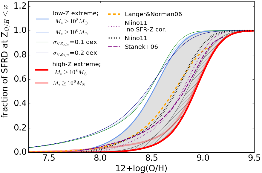
Figure 13: Cumulative fractions of total star formation at z$\sim$0 happening below a certain metallicity. The solid lines show the results from our study (thick $-$ high-Z extreme, thin $-$ low-Z extreme) using galaxies with $M_{*}\geq 10^{8}{\rm~{}M}_{\odot}$ (dark lines) or $M_{*}\geq 10^{6}{\rm~{}M}_{\odot}$ (faint lines). The gray area spans between the two extremes for the $M_{*}\geq 10^{8}{\rm~{}M}_{\odot}$ mass cut. The thin lines around the left-most extreme demonstrate the effect of varying the metallicity dispersion ($\sigma_{\nabla O/H}$) within galaxies between 0.1 dex (steeper curve) and 0.2 dex (flatter curve). The hatched region on the right demonstrates the effect of changes in the SFMR only (the right edge $-$ no flattening, the left edge $-$ sharp flattening in the SFMR).
We overplot the results from Stanek et al. (2006), Niino (2011) and based on the method from Langer & Norman (2006). Despite the different assumptions, those results fall between the range indicated by the extreme cases identified in our study.

Several other studies used empirical scaling relations for star forming galaxies to obtain the information about the distribution of the star formation (or the formation of transients related to massive stars) across different metallicities. Below we highlight the similarities and differences with respect to our method. The details of the different methods are summarized in Tab. 6 in appendix F. We note that none of those studies set finding the SFRD(Z,z) distribution as its main goal and only a very limited comparison of our results with the published material is possible.

Stanek et al. (2006) and Niino (2011) limited their analysis to low redshifts ($z\lesssim$0.3) and focused on application to long GRBs. Both studies take into account the intrinsic scatter in the SFMR and MZR. Stanek et al. (2006) does not take into account the correlation between the SFR and metallicity due to FMR, while Niino (2011) shows a variation in which they use the FMR from Mannucci et al. (2011) instead of combining the SFMR and MZR. Stanek et al. (2006) consider two variations of the high-mass end slope of the SFMR - relation with a downturn (also used by Niino 2011, see Fig. 1 therein) and relation with flattening (similar to our sharp flattening case). We note that such a downturn has not been observed in any of the subsequent studies of the SFMR. This assumption may underestimate the star formation happening at high metallicities.

Dominik et al. (2013) and Langer & Norman (2006) use a slightly different approach than presented in this study: they first obtain the metallicity distribution at each redshift (convolving MZR and GSMF) and scale it with SFRD(z) to obtain the SFRD(Z,z) . Those authors constructed the $SFRD(Z,z)$ that can be extended to high redshifts, albeit with various simplifications. One of them is that the adopted mass metallicity relation assumes no scatter so that there is a unique correspondence between mass and metallicity, and the redshift evolution only affects the normalization of the relation. Furthermore, both methods implicitly assume a constant specific star formation rate (i.e. $SFR(M_{\ast})\propto M_{\ast}$; this is similar to our ’no flattening’ case but with a different slope) at all redshifts. They do not account for the FMR.
Dominik et al. (2013) use MZR with the functional from Tremonti et al. (2004) and redshift-dependent normalization, adjusted to produce average metallicity of galaxies at $z=0$ of $Z$=0.03 or 0.016 in their high-end and low-end model respectively (see Fig. 2 therein). Langer & Norman (2006) use a non-evolving GSMF and assume that the MZR is a single power law (without the observed flattening at high $M_{*}$) and its normalization decreases with redshift (at $z\gtrsim$2 the decrease is much slower than in any variation considered in our study).
Note that the assumed lack of flattening in MZR (and possibly SFMR) does likely not affect the results of studies that use only the low-metallicity part of the distribution (as in some application to long GRB e.g. Langer & Norman 2006), but may be important for other applications (e.g. the model by Langer & Norman 2006 has been recently used by to calculate the merger rates of double compact objects in Barrett et al. 2018; Eldridge et al. 2019, this was also the application of the model by Dominik et al. 2013).

Another example of using scaling relations to infer the information about metallicity comes from Madau & Fragos (2017). However, the authors give only the mass-averaged mean gas-phase metallicity and not the entire distribution. They use the mass-metallicity relation from Zahid et al. (2014) and GSMF from several studies to estimate the mean at different redshifts, assuming that the relation given by Zahid et al. (2014) can be extrapolated to z$\sim$7. The resulting mass-averaged mean metallicity is overplotted in Fig. 6 showing our moderate variation. This mean is very close to the peak metallicity in the high metallicity extreme (note that the MZR assumed in Madau & Fragos (2017) is based on KK04 calibration, as in the high-Z extreme case) from our study at $z\lesssim$3 and is significantly higher at higher redshifts.

Using the results from Langer & Norman (2006), we construct the cumulative distribution of total star formation below a certain metallicity for their method and plot it in Fig. 13 together with the ones from Stanek et al. (2006) (Fig. 2 therein, thick solid line), Niino (2011) (Fig. 4 and 5 therein, solid lines) and resulting from our model. It can be seen that all the curves fall within the broad range defined by the extreme cases from our study (gray area). The hatched region shows how much the result would change only due to changes in the SFMR on the example of the high-Z extreme model variation. The width of this range is much smaller than the width of the gray area, which shows that it is mostly set by the differences in the MZR. The results from Niino (2011) were obtained for the same metallicity calibration as assumed in the high-Z extreme case. They reveal a noticeably greater offset towards low metallicities from the high-Z extreme curve than indicated by the hatched region, especially if the correlation between the SFR and $Z_{O/H}$ is accounted for (as in our model). This difference may be (partially) explained by the high-mass turnover in the SFMR used by Niino (2011), although as discussed earlier in this section, there are also other differences in the assumptions between our study and Niino (2011).
Based on the data shown in the bottom panel of Fig. 2 from Dominik et al. (2013), we conclude that their low-end model would fall well within the gray area shown in Fig. 13. However, the high-end model from Dominik et al. (2013) predicts hardly any $z\sim$0 star formation below $Z_{O/H}\sim$8.7 (see the middle panel in Fig. 2 therein) and therefore the cumulative distribution of the total star formation below certain $Z_{O/H}$ for that model would be shifted to noticeably higher metallicities with respect to our high-Z extreme shown in Fig. 13.

7 Conclusions

We combine empirical scaling relations for star forming galaxies over wide range of masses and redshifts and other observational properties of those galaxies to address the question of (i) how was the cosmic star formation rate density distributed over metallicities throughout the history of the Universe (SFRD(Z,z)) and (ii) how uncertain is that distribution given the currently unresolved problems concerning the observationally inferred scaling relations.
To evaluate the uncertainty of the SFRD(Z,z) obtained with our method, we use different versions of the scaling relations, covering the range of possibilities present in the literature. We use four different versions of the mass $-$ metallicity relations (based on different metallicity calibrations; with different normalizations, shapes and evolution with redshift), vary the assumptions about the high mass end of the star formation $-$ mass relation (assuming either a single power law, broken power law or sharp flattening at the high mass end) and about the low mass end of the galaxy stellar mass function (assuming a fixed low mass end slope or a slope that steepens with redshift). We take into account the scatter present in the relations, the observed correlation between the SFR and metallicity (the fundamental metallicity relation) and the distribution of gas metallicity within galaxies. We extend the analysis up to $z\sim$10, but we note that the MZR is not constrained by observations above $z\sim$3.5 and hence our results at higher redshifts rely on extrapolations. To quantify the differences between the variations of our model, we compare the fractions of stellar mass formed at low (below 10% solar) and high (above solar) metallicity at $z\leq$0.5, 3 and 10. Our main results can be summarized as follows:

• We identify two variations $-$ the low and high metallicity extremes $-$ that maximize the fraction of stellar mass formed at low and high metallicity respectively. Those extremes are reached by combining the $PP04$ MZR (based on the Pettini & Pagel 2004 O3N2 metallicity calibration) with the SFMR with sharp flattening at high masses in the low-Z extreme case and $KK04$ MZR (based on the Kobulnicky & Kewley 2004 metallicity calibration) with the SFMR with no flattening at high masses in the high-Z extreme. The fraction of mass formed in stars at low (high) metallicity since $z$=3 differs by $\sim$18% ($\sim$26%) between the two extremes. Those two variations also lead to different total stellar mass formed at each redshift (with the higher stellar mass formed in the high-Z extreme). This reduces the difference between the extremes if the stellar mass (instead of the fraction) formed at low metallicity is considered and increases the difference between the amount of stellar mass formed at high metallicity.

• We find that the variations with the low mass end slope of the GSMF that steepens with redshift significantly overpredict the total star formation rate density at $z\gtrsim$4 with respect to other observational estimates. The cause of this discrepancy is not clear. Those variations were not considered at $z\gtrsim$4.

• The differences between the MZRs obtained for different metallicity calibrations (in particular the differences in normalization) are the main cause of uncertainty in our results at $z\lesssim$4.

• We compare the results from our model with the local specific core-collapse supernovae (CCSN) rate as a function of metallicity from Graur et al. (2017). The uncertainties in the CCSN-location metallicity estimates, as well as in the translation of the total SFR to the number of CCSN do not allow us to draw any strong conclusions from that comparison. However, it might suggest that the variations with the sharp flattening at the high mass end of the SFMR underestimate the local high metallicity star formation. The other variations of our model show a reasonably good agreement with the data.

Our model is publicly available and can be used in studies focusing on the properties of populations of systems composed of stars and their remnants, stellar-evolution related transients and their likely environments. In particular, it can be applied to calculate the rates of those transients and to evaluate their uncertainty due to the assumed distribution of the cosmic star formation rate density across metallicities and redshifts. It can also serve for comparison for the cosmological simulations.

Appendix A Metallicity $-$ nomenclature and solar composition

The term ‘metallicity‘ has been used variously in the literature, depending on the object of interest and the method used. It is generally understood as a measure of the abundance of metals (elements heavier than helium) in a certain object or system and defined as a fraction of total baryonic mass contained in metals:

$$Z\equiv\frac{M_{metals}}{M_{baryons}}$$ (5)

although this definition is mostly applicable in theoretical studies. Observationally metallicity is often expressed in terms of the of the oxygen to hydrogen abundance ratio:

$$Z_{O/H}\equiv 12+\rm log\left(O/H\right)\equiv 12+log\left(n_{O}/n_{H}\right)$$ (6)

where $n_{i}$ stands for the number density of either oxygen or hydrogen. This definition is commonly used e.g. in interstellar medium studies, since oxygen is the most abundant heavy element and it is relatively easy to observe due to its strong optical lines. The common assumption is that the other elements scale linearly with the measured $Z_{O/H}$ maintaining the solar abundance ratios (so that the conversion between the two measures has the form: $log\left(Z/Z_{\odot}\right)=Z_{O/H}-Z_{O/H\odot}$, where $Z_{\odot}$ and $Z_{O/H\odot}$ stand for the solar metallicity in both measures).
However, the exact value of solar metallicity and solar composition is presently unknown. For instance, a widely used result obtained by Asplund et al. (2009) based on 3D modeling of the solar atmosphere gives $Z_{\odot}$=0.0134 and $Z_{O/H\odot}$=8.69. Such low values of metallicity made it difficult to recover the helioseismically inferred information about the solar interior, such as sound speed profile, the location of the convective zone boundary and surface helium abundance (e.g. Serenelli et al., 2009; Serenelli, 2016). In fact, the metallicity estimates based on helioseismology are systematically higher, with $Z_{O/H\odot}\sim$8.85 (e.g. Delahaye & Pinsonneault, 2006; Villante et al., 2014). Using the abundances found by Villante et al. (2014), the resulting $Z_{\odot}\approx$0.019. Similarly high values were obtained by the earlier solar atmosphere studies, e.g. Anders & Grevesse (1989) found $Z_{O/H\odot}$=8.83 and Grevesse & Sauval (1998) found $Z_{O/H\odot}$=8.93. Asplund et al. (2009) recalculated $Z_{\odot}$ from those studied using the updated He abundances from helioseismology and found $Z_{\odot}$=0.017 and $Z_{\odot}$=0.0201 respectively.

Appendix B Initial mass function - corrections

The choice of a particular IMF impacts the estimates of both stellar masses and star formation rates inferred from observations and as a result affects all of the galaxy scaling relations used in our model. The results obtained assuming a certain IMF can be translated to another IMF by shifting the mass and SFR estimates by a certain value (the change is in the same direction, but generally with different magnitude). To correct for differences between the IMFs used in various studies (either Salpeter (1955), Kroupa (2001) or Chabrier (2003)) we use the correction factors listed in table 5, unless explicitly stated otherwise. These include the mass conversions as given in Speagle et al. (2014) (see eq. 2 therein) and simple SFR correction calculated as the ratio of the total mass in both IMFs assuming the same number of massive stars ($>$10 ${\rm~{}M}_{\odot}$ $-$ stars that are responsible for the bulk of the measured UV light; e.g. Boogaard et al., 2018; Fermi-LAT Collaboration et al., 2018).

Table 5: conversion factors used in this study to correct for different IMFs used in various studies; Kroupa (2001): K01, Chabrier (2003): Ch03, Salpeter (1955): Sal.
Mass correction from IMF1 to IMF2: $\rm log\left(M_{IMF2}\right)=log\left(M_{IMF1}\right)+\Delta log(M)$
SFR correction from IMF1 to IMF2: $\rm SFR_{IMF2}=SFR_{IMF1}\times K_{IMF}$

conversion factor	K01 to Sal	K01 to Ch03
$\Delta$log(M)	+0.21 dex	$-$ 0.03 dex
$K_{IMF}$	1.5	0.94

Appendix C Metallicity of stars - differences between the variations

C.1 The metallicity at which the most of the stellar mass was formed

As discussed in Sec. 4.2.2, in almost all cases discussed in our study most of the stellar mass forms outside the assumed low and high metallicity regimes (i.e. between 0.1 ${\rm~{}Z}_{\odot}$ and ${\rm~{}Z}_{\odot}$). Here we look at the exact location of the peak of the distribution of mass formed in stars across metallicities for different redshift ranges and discuss its dependence on the assumptions about the MZR, SFMR and GSMF.
Figure 14 shows an example of such distribution. We note that for all the variations considered in our study such distributions can be described by a combination of a left-skewed normal distribution and a power-law tail at low $Z_{O/H}$. When higher redshifts are included, the peak of the skewed-normal part shifts towards lower metallicities and the distribution broadens on the low metallicity side while the tail builds up.

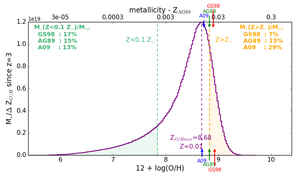
Figure 14: Distribution of the mass formed in stars since redshift z=3 at different metallicities (measured in oxygen to hydrogen abundance 12 + log(O/H) $-$ bottom scale, or as a metal mass fraction $-$ top scale) for the model assuming moderate flattening at the high mass end of SFMR, M09 mass metallicity relation and $\alpha_{fix}$=$-$1.45 (SFRD(Z,z) for that variation is shown in Fig. 6). The green tail of the distribution corresponds to the stars forming at $Z<0.1\ {\rm~{}Z}_{\odot}$, while the orange one at $Z>{\rm~{}Z}_{\odot}$. The purple line indicates the peak of the distribution. This variation of the model falls in between the extreme cases in terms of the fraction of low and high metallicity star formation. The fractions of mass formed in stars at $Z<0.1\ {\rm~{}Z}_{\odot}$ and $Z>{\rm~{}Z}_{\odot}$ for the discussed model are given in the top left and top right corner of the figure respectively, for the three commonly used solar metallicity estimates. In this paper we assume Anders & Grevesse (1989) solar metallicity (AG89; indicated with the green arrows) and the top scale was calculated from 12 + log(O/H) using the solar abundances found by these authors. The other two commonly adopted solar metallicity estimates are indicated with blue (A09; Asplund et al., 2009) and red (GS98; Grevesse & Sauval, 1998) arrows for the reference.

The peak metallicity for different model variations is shown in Fig. 15. It shows relatively little dependence on the assumed shape of the high mass part of the SFMR. This can be seen by comparing at the location of the symbols with the same colour and different shapes in Fig. 15. The difference is $\sim$0.1 dex. Comparing points plotted with the same symbol and colour but with and without edge in Fig. 15 we conclude that the effect of the low mass end slope of the GSMF is negligible. To investigate the effect of the assumed mass metallicity relation (MZRs obtained for different metallicity calibrations), we compare the locations of points plotted with the same symbol but with different colours. It can be seen that for the T04, KK04 and M09 MZRs the difference is within 0.1 dex. Those three relations have similar (high) normalizations at z$\sim$0. Additionally, both the M09 and T04 relations are relatively steep and evolve with redshift at a similar rate and hence the green and blue points corresponding to those relations can be found close to each other or they even overlap in Fig. 15. The KK04 MZR is flatter than those two relations (so that according to this MZR low mass galaxies have higher metallicities compared to M09 or T04) and shows a milder redshift evolution and its peak metallicity is the highest. The peak metallicity obtained for the PP04 MZR (with the low initial normalization) falls $\gtrsim$0.25 dex below the other three MZRs.

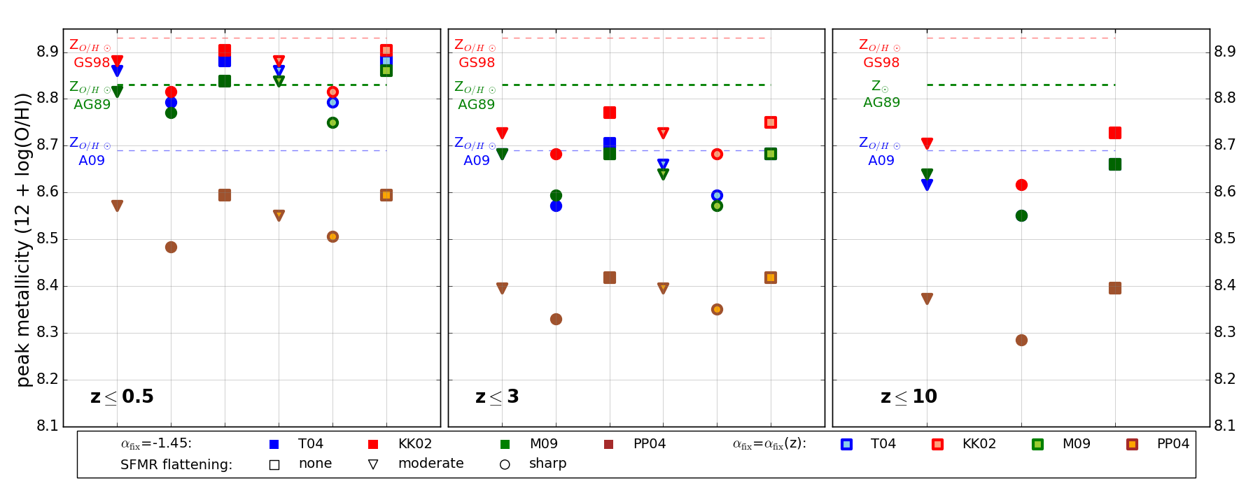
Figure 15: 12 + log(O/H) at the peak of the distribution of mass formed in stars at different metallicities (see Figure 14) since redshift z=0.5 (left), z=3 (middle) and z=10 (right) for different variations of the model. Different symbols correspond to the assumptions about the high mass part of the SFMR: squares $-$ no flattening, triangles $-$ moderate flattening, circles $-$ sharp flattening. Colours distinguish different assumptions about the MZR and low mass end slope of the GSMF. The dark colours correspond to $\alpha_{fix}$=$-$1.45, where the MZRs are: blue $-$ T04, red $-$ KK04, green $-$ M09, brown $-$ PP04; The symbols with contours and light colours correspond to $\alpha_{fix}=\alpha_{fix}(z)$ steepening with redshift, where the MZRs are light blue $-$ T04, light red $-$ KK04, light green $-$ M09, orange $-$ PP04. We exclude the variations with $\alpha_{fix}(z)$ at high redshifts z$\gtrsim$4 (see text). The solar oxygen abundance estimates from Anders & Grevesse (1989) (AG89; green), Asplund et al. (2009) (A09; blue) and (Grevesse & Sauval, 1998) (GS98; red) are indicated with the horizontal dashed lines for the reference.

C.2 Low metallicity mass fraction

The fraction of mass formed in stars at low metallicities since $z$=0.5, 3 and 10 for different variations of the model is shown in Fig. 16. The choice of the MZR (or metallicity calibration) has a decisive role in setting the fraction of the low metallicity star formation (compare the same symbols plotted with different colours). As expected, this fraction is the highest for PP04 (brown) and the lowest for the KK04 MZR (red) at all redshifts.
The second important factor is the flattening at the high mass end of the SFMR. For a given MZR (fixed colour in Fig. 16) the sharp flattening case (circles) leads to the highest fraction of mass formed at low metallicity and this fraction is the lowest if the SFMR is a single power-law (‘no flattening‘ case; squares).
The evolving low mass end slope of GSMF leads to a slight increase in the amount of mass formed at low $Z_{O/H}$ since $z$=3 with respect to the fixed slope case (as there are more low mass galaxies forming low metallicity stars). This variation is not considered at higher redshift for the reasons discussed in sec. 4.1.1.

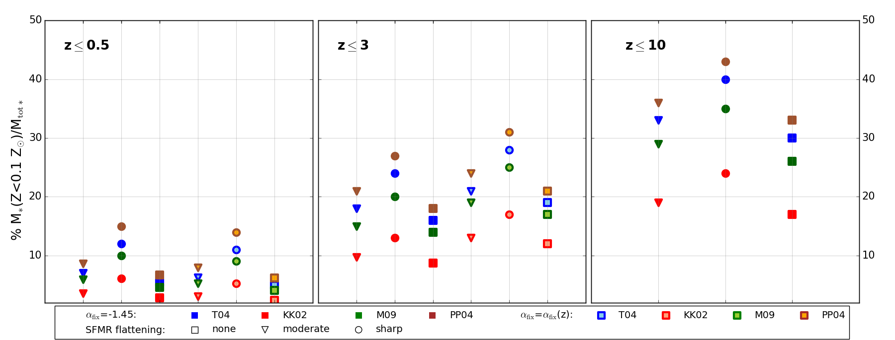
Figure 16: The fraction of mass formed in stars at low metallicities ($<0.1{\rm~{}Z}_{\odot}$; calculated assuming solar metallicity from Anders & Grevesse, 1989) since redshift z=0.5 (left), z=3 (middle) and z=10 (right) for different variations of the model. Different symbols correspond to the assumptions about the high mass part of the SFMR: squares $-$ no flattening, triangles $-$ moderate flattening, circles $-$ sharp flattening. Colours distinguish different assumptions about the MZR and low mass end slope of the GSMF. The dark colours correspond to $\alpha_{fix}$=$-$1.45, where the MZRs are: blue $-$ T04, red $-$ KK04, green $-$ M09, brown $-$ PP04; The symbols with contours and light colours correspond to $\alpha_{fix}=\alpha_{fix}(z)$ steepening with redshift, where the MZRs are light blue $-$ T04, light red $-$ KK04, light green $-$ M09, orange $-$ PP04. We exclude the variations with $\alpha_{fix}(z)$ at high redshifts z$\gtrsim$4 (see text).

Appendix D Comparison with core-collapse supernovae rates

D.1 Cosmic SFRD vs CCSN rate density

It is commonly assumed that the CCSN rate is proportional to the SFR and the constant of proportionality depends solely on the IMF and can be estimated as a number of stars that explode as CCSNe per unit mass (the efficiency of formation of CCSN progenitors; e.g. equation 16 in Madau & Dickinson, 2014). This calculation requires assuming a certain initial mass range for the progenitors of CCSNe. However, the exact limits of this mass range are not known (and the range itself may in fact consist of so-called islands of explodability, e.g. Sukhbold & Woosley, 2014; Pejcha & Thompson, 2015; Sukhbold et al., 2016). Furthermore, those limits depend on the stellar metallicity (e.g. Heger et al., 2003; Langer, 2012; Doherty et al., 2015) and hence likely change throughout the cosmic history. The expected CCSN progenitor mass range is further modified by binary interactions and stellar mergers (e.g. Eldridge et al., 2008; Zapartas et al., 2017). As argued by Sana et al. (2012), over 70% of the most massive stars are born in interacting binary systems and $\sim$20 $-$ 30% will experience a merger with their companion. Stellar interactions and mergers can act both to reduce the number of CCSN expected from a certain stellar population (e.g. by mergers of two CCSNe progenitors) and to increase that number (e.g. by mergers of the more common low mass stars that result in a CCSN progenitor). Zapartas et al. (2017) find that the overall effect of accounting for the binaries is to increase the number of the CCSN expected to form from a stellar population of the same mass (they find $\sim$14% increase, although the exact number is model dependent). Another complication added by binaries is the fact that for the same amount of star formation, stellar population containing binaries would lead to a higher UV luminosity than the one consisting only of single stars and therefore would lead to an overestimate in the SFR measured using the common UV-light based tracers (e.g. Xiao & Eldridge, 2015, the magnitude of this effect varies depending on the SFR tracer and metallicity of the stellar population). In other words, the actual number of stars born as CCSN progenitors would be smaller than what results from the inferred SFR, which would lead to an overestimate of the number of expected CCSN. The combined effect of the presence of binaries in the observed stellar population on the CCSN formation efficiency is not clear. The comparison is further complicated by the fact that the observational CCSN rate estimates are not always consistent with each other, which may be partially attributed to different methods used to correct for the number of CCSN missed due to obscuration by dust (e.g. Graur et al., 2015).

D.2 Central metallicity vs metallicity at the supernova location

Galbany et al. (2016) suggest that the true metallicity at the CCSN location should be contained within the range reaching metallicity 0.1 dex lower than the central value. However, the Marino et al. (2013) metallicity calibration used in Galbany et al. (2016) probes a relatively small metallicity range and as shown in Sánchez-Menguiano et al. (2016), leads to relatively flat metallicity gradient estimates. For instance, Sánchez-Menguiano et al. (2016) find the typical metallicity gradient of around $-$0.07 dex/r_e using the Marino et al. (2013) calibration, $-$0.11 dex/r_e with the PP04 calibration and $-$0.14 dex/r_e using the theoretical calibration from Dopita et al. (2013). Hence, based on the metallicity gradient studies and taking this into account the fact that CCSN are found to explode within 2 r_e from the centre, (with an average distance of around 1 r_e, e.g. Galbany et al., 2016), one can expect to find also larger offsets between the central and local metallicity than 0.1 dex proposed by Galbany et al. (2016) (especially when using one of the theoretical metallicity calibrations). Sanders et al. (2012) find a median offset between the nuclear and explosion site metallicity for their stripped envelope SN sample of $\sim$0.08 dex in the PP04 scale, although with a substantial scatter (see Fig. 12 therein). However, the galaxies considered in this study contain objects at higher redshift and with smaller angular sizes than those used in Graur et al. (2017). Hence, the nuclear metallicity in those galaxies was measured with a larger covering fraction (averaging information from a larger portion of the galaxy) and can be expected to be closer to the metallicity at the SN explosion site. Modjaz et al. (2011) compared the local metallicities of part of their sample of stripped envelope supernovae with the central metallicities obtained from the nuclear SDSS spectra using the PP04 metallicity scale and found the average difference of 0.13 dex and in the extreme cases reaching up to 0.24 dex.

D.3 Specific CCSN rate vs metallicity - dependence on the scatter in metallicity

The shape of the dependence of the specific CCSN rate on metallicity is a consequence of the scaling relations in star forming galaxies. The specific star formation rate (SFR/$M_{\ast}$) decreases with mass, so that there are fewer CCSN per stellar mass in more massive host galaxies. The mass - metallicity relation tells that with the increasing stellar mass (and hence decreasing specific SFR or specific CCSN rate) metallicity increases up to a certain $Z_{O/H}$ value, at which the MZR flattens, hence the slope of the specific CCSN rate $-$ metallicity relation steepens around the metallicity at which the MZR begins to flatten. The presence of the scatter around the MZR pushes a fraction of the star formation into higher and lower metallicity than what results from the MZR, but the anticorrelation between the SFR and metallicity (resulting from the fundamental metallicity relation) reduces that ‘smearing‘ effect of the scatter and acts to further steepen the high-metallicity slope. The gray solid line in Fig. 11 shows the specific CCSN rate $-$ metallicity relation when only the scatter in the MZR ($\sigma_{0}$) is taken into account. It can be seen that the high-metallicity slope of the gray curve is steeper than in the case of the blue solid curve, which corresponds to the same model variation, but taking into account the fact that the stars within galaxies can form with a range of metallicities ($\sigma_{\nabla O/H}$=0.14 dex). Hence, the assumed width of this distribution has a noticeable effect on the high metallicity end slope and on the location of the turnover in the specific CCSN rate $-$ metallicity dependence.
For instance, the power law slope of the high metallicity Z${}_{O/H}\gtrsim 8.5$ part of this relation is $\sim$ $-$1 for $\sigma_{\nabla O/H}$=0.14 dex, $\sim$ $-$1.4 for $\sigma_{\nabla O/H}$=0.1 dex and for $\sim$ $-$0.65 for $\sigma_{\nabla O/H}$=0.2 dex.

Appendix E Closer look at the secondary assumptions

E.1 The distribution of the star formation over metallicities within galaxies

As discussed in Sec. 2.3.3, there is a range of metallicities at which stars form within their host galaxies.
Our treatment of the distribution of metallicity of the star formation within galaxies is very simplified. We assume that it can be described as a normal distribution centered at the metallicity resulting from the MZR (taking into account the anticorrelation between the metallicity and the SFR) and with a dispersion $\sigma_{\nabla O/H}$=0.14 dex for all galaxies and redshifts and irrespective of the choice of the MZR (metallicity calibration).
However, the range of metallicities found in the HII regions (setting the width of the distribution), as well as the value of the characteristic metallicity gradient depend on the assumed metallicity calibration (e.g. Sánchez-Menguiano et al., 2016). The value of $\sigma_{\nabla O/H}$ that we use is based on the averaged results obtained using the Marino et al. (2013) and the Pettini & Pagel (2004) metallicity calibrations and could be higher if different (theoretical) metallicity calibrations were used.
On the other hand, the offsets between the metallicities measured at the location of the CCSN and the central metallicity of its host galaxies (which also indicate the range of metallicities at which the stars form within galaxies) reported in the studies using the empirical metallicity calibrations mentioned above are smaller than 2$\times\sigma_{\nabla O/H}$ (see appendix D.2 and references therein).
Furthermore, not all galaxies reveal a single slope negative metallicity gradient. (Carton et al., 2018) studied galaxies at intermediate redshifts and found a significant fraction of galaxies showing gradients that are consistent with being flat and several cases of positive gradients, which might suggest that the simple common negative metallicity gradient found in the galaxies in local Universe may not be relevant at higher redshifts.
Finally, the detailed studies of metallicity gradients within galaxies (on which we based our assumptions) are limited to the relatively local Universe. It is thus relevant to ask how much our results depend on this particular assumption.

E.1.1 The importance for our results

To asses the importance of the assumptions about the distribution of the star formation over metallicities within galaxies on our results, we vary the value of $\sigma_{\nabla O/H}$ in the range 0.1$-$0.2 dex. The effect on the results (summarized in Table 4) is minor: the difference in the total stellar mass formed and the fraction of the low metallicity star formation is negligible and the fraction of the high metallicity star formation differs by less than 3% between the calculations with $\sigma_{\nabla O/H}$=0.1 and 0.2 dex for all model variations. The distribution of mass formed in stars at different metallicities since a certain redshift (see Fig. 14) slightly broadens as $\sigma_{\nabla O/H}$ increases, however this broadening only affects the low metallicity (Z$<0.1{\rm~{}Z}_{\odot}$) tail of the distribution at high redshifts $z>$5. At the same time the peak metallicity shifts to lower values (by less than 0.03 dex for the distribution at z$<$0.5 and less than 0.09 dex at z$<$10 for all model variations), which reduces the impact of the broadening on the fraction of the high metallicity star formation. However, as discussed in Sec. 5, changing $\sigma_{\nabla O/H}$ noticeably affects the slope of the high metallicity end of the specific CCSN rate $-$ metallicity relation (see Fig. 11 and Sec. D.3).

E.2 Contribution from passive galaxies

In this study we use the scaling relations and galaxy mass functions obtained for star forming galaxies. However, various criteria to select those galaxies are used in the literature and a fraction of galaxies classified as passive may still have some residual star formation. The fraction of passive galaxies increases towards lower redshifts (e.g. Muzzin et al., 2013; Davidzon et al., 2017) and hence their contribution to the global star formation budget can be expected to be the highest in the local Universe. Renzini & Peng (2015) use the SDSS DR7 release data to study the star formation $-$ mass relation of the local galaxies without imposing any cuts on the star formation within galaxies in their sample, i.e. including quenched galaxies. They find that a low level of star formation is still present within the passive population (although they note that in many cases the measured SFR may be an upper limit) and show that while the majority of mass in the local Universe reside in those galaxies, they do not contribute significantly to the ongoing star formation.

E.2.1 Importance for our results

To obtain a rough estimate of the upper limit on the local star formation rate density contributed by passive galaxies, we construct the ‘upper limit star formation $-$ mass relation‘ for passive galaxies by fitting a line connecting the two low SFR peaks in the SFR $-$ stellar mass plane shown in Fig. 4 in Renzini & Peng (2015). Combining it with the local galaxy stellar mass function for the passive (red) population of galaxies from Baldry et al. (2012) and integrating over the stellar masses between $10^{8}-10^{12}{\rm~{}M}_{\odot}$, we find that the contribution of passive galaxies to the local SFRD is more than a factor of 80 smaller than the SFRD obtained for the star forming galaxies in that mass range in the moderate variation of our model. Most of this residual star formation occurs in massive galaxies and hence adds to the high metallicity tail of the SFRD(Z,z) distribution. Assuming that all the star formation from passive galaxies adds to the star formation at Z$>{\rm~{}Z}_{\odot}$ and their contribution to the global SFRD is at the level corresponding to the estimated upper limit, the fraction of mass formed in stars at high metallicity at $z<0.5$ in the moderate variation of our model would increase by $\lesssim$1%. Taking into account the fact that the fraction of passive galaxies decreases with redshift, only some of them show some residual star formation and the above estimate used the upper limit on the level of that residual star formation rate, we conclude that the omitted star formation in passive galaxies has negligible effect on our results.

Appendix F SFRD(Z,z) from scaling relations - other studies

Table 6 summarizes the assumptions made by several different authors using empirical (or mixed empirical and theoretical/simulated) scaling relations to infer SFRD(Z,z).

Table 6: Summary of the assumptions made by different authors using empirical (or mixed empirical and theoretical/simulated e.g. Dominik et al. 2013, Neijssel et al. 2019) scaling relations to infer SFRD(Z,z). In the row ’method’ we indicate whether the authors combine SFMR, MZR & GSMF (as in our study) or convolve MZR & GSMF to obtain metallicity distribution (as a function of $z$) and obtain the scaling using SFRD(z).
’+’: included as a variation
ⁱ: Dominik et al. (2013) use MZR with the functional from Tremonti et al. (2004) and redshift-dependent normalization. The normalization is calculated based on the results from Pei et al. (1999) and Young & Fryer (2007) and subsequently adjusted to produce average metallicity of galaxies at z = 0 of 1.5 ${\rm~{}Z}_{\odot}$ or 0.8 ${\rm~{}Z}_{\odot}$ in their high-end and low-end model respectively (see Fig. 2 therein, note that ${\rm~{}Z}_{\odot}$=0.02 in Dominik et al. 2013).
ⁱⁱ: see Fig. 1 in Niino (2011)
ⁱⁱⁱ: in their fiducial model; the distribution of metallicity at each redshift is described as a log-normal distribution with $\sigma$=0.39 dex
^iv: Furlong et al. (2015) - fit to $z$ evolution (cosmological simulations); Panter et al. (2004) - non-evolving

study:	Stanek et al. (2006)	Niino (2011)	Langer & Norman (2006)	Dominik et al. (2013)	Neijssel et al. (2019)
method:	SFMR, MZR & GSMF	SFMR, MZR & GSMF	SFRD(z), MZR & GSMF	SFRD(z), MZR & GSMF	SFRD(z), MZR & GSMF
$z$	$\lesssim$0.25	$\lesssim$ 0.3	$\lesssim$10	$\lesssim$10	$\lesssim$6
log($M_{*}/{\rm~{}M}_{\odot}$)	$>$7.4	$>$8	-	$>$7	-
MZR					+Savaglio et al. (2005)
	T04	KK04	single power law	modified T04i	+Ma et al. (2016)
					+Langer & Norman (2006)
MZR(z)	-	-	normalization	decreasing	normalization
	-	-	-0.15 dex per $\Delta z$=1	normalizationi	-0.23 dex per $\Delta z$=1iii
$\sigma_{\rm MZR}$	0.1 dex	0.1 dex	-	-	- / 0.39 dexiii
GSMF	Bell et al. (2003)	Bell et al. (2003)	Panter et al. (2004)	Fontana et al. (2006)	+Panter et al. (2004)
				(fit to $z$ evolution)	+Furlong et al. (2015)
	non-evolving	non-evolving	non-evolving	non-evolving at $z>$4	variousiv
SFMR	Brinchmann et al. (2004)	Brinchmann et al. (2004)	$\sim$const. specific SFR	$\sim$const. specific SFR	$\sim$const. specific SFR
	(downturn at high M∗)ii	(downturn at high M∗)ii	SFR(M∗)$\propto$M∗	SFR(M∗)$\propto$M∗	SFR(M∗)$\propto$M∗
	+: sharp flattening
$\sigma_{SFR}$	0.3 dex	0.3 dex	-	-	-
FMR	-	+: Mannucci et al. (2011)	-	-	-
$\sigma_{\nabla Z_{O/H}}$	-	+0.1/0.3/0.5 dex	-	-	-

References

- Anders & Grevesse (1989) Anders E., Grevesse N., 1989, Geochimica Cosmochimica Acta, 53, 197
- Andrews & Martini (2013) Andrews B. H., Martini P., 2013, ApJ, 765, 140
- Asplund et al. (2009) Asplund M., Grevesse N., Sauval A. J., Scott P., 2009, ARA&A, 47, 481
- Atek et al. (2018) Atek H., Richard J., Kneib J.-P., Schaerer D., 2018, MNRAS, 479, 5184
- Baldry et al. (2004) Baldry I. K., Glazebrook K., Brinkmann J., Ivezić Ž., Lupton R. H., Nichol R. C., Szalay A. S., 2004, ApJ, 600, 681
- Baldry et al. (2012) Baldry I. K., et al., 2012, MNRAS, 421, 621
- Barber et al. (2018) Barber C., Crain R. A., Schaye J., 2018, MNRAS, 479, 5448
- Barber et al. (2019) Barber C., Schaye J., Crain R. A., 2019, MNRAS, 483, 985
- Barrett et al. (2018) Barrett J. W., Gaebel S. M., Neijssel C. J., Vigna-Gómez A., Stevenson S., Berry C. P. L., Farr W. M., Mandel I., 2018, MNRAS, 477, 4685
- Bastian et al. (2010) Bastian N., Covey K. R., Meyer M. R., 2010, ARA&A, 48, 339
- Belczynski et al. (2010) Belczynski K., Dominik M., Bulik T., O’Shaughnessy R., Fryer C., Holz D. E., 2010, ApJ, 715, L138
- Belczynski et al. (2016) Belczynski K., Holz D. E., Bulik T., O’Shaughnessy R., 2016, Nature, 534, 512
- Bell et al. (2003) Bell E. F., McIntosh D. H., Katz N., Weinberg M. D., 2003, ApJS, 149, 289
- Bhatawdekar et al. (2019) Bhatawdekar R., Conselice C. J., Margalef-Bentabol B., Duncan K., 2019, MNRAS, 486, 3805
- Bignone et al. (2017) Bignone L. A., Tissera P. B., Pellizza L. J., 2017, MNRAS, 469, 4921
- Bisigello et al. (2018) Bisigello L., Caputi K. I., Grogin N., Koekemoer A., 2018, A&A, 609, A82
- Boogaard et al. (2018) Boogaard L. A., et al., 2018, A&A, 619, A27
- Botticella et al. (2008) Botticella M. T., et al., 2008, A&A, 479, 49
- Bouwens et al. (2015) Bouwens R. J., et al., 2015, ApJ, 803, 34
- Bouwens et al. (2017) Bouwens R. J., Oesch P. A., Illingworth G. D., Ellis R. S., Stefanon M., 2017, ApJ, 843, 129
- Bresolin (2007) Bresolin F., 2007, ApJ, 656, 186
- Bresolin et al. (2016) Bresolin F., Kudritzki R.-P., Urbaneja M. A., Gieren W., Ho I.-T., Pietrzyński G., 2016, ApJ, 830, 64
- Brinchmann et al. (2004) Brinchmann J., Charlot S., White S. D. M., Tremonti C., Kauffmann G., Heckman T., Brinkmann J., 2004, MNRAS, 351, 1151
- Brinchmann et al. (2008) Brinchmann J., Pettini M., Charlot S., 2008, MNRAS, 385, 769
- Cappellaro et al. (2015) Cappellaro E., et al., 2015, A&A, 584, A62
- Carton et al. (2018) Carton D., et al., 2018, MNRAS, 478, 4293
- Chabrier (2003) Chabrier G., 2003, PASP, 115, 763
- Chruslinska et al. (2019) Chruslinska M., Nelemans G., Belczynski K., 2019, MNRAS, 482, 5012
- Conselice et al. (2016) Conselice C. J., Wilkinson A., Duncan K., Mortlock A., 2016, ApJ, 830, 83
- Dahlen et al. (2012) Dahlen T., Strolger L.-G., Riess A. G., Mattila S., Kankare E., Mobasher B., 2012, ApJ, 757, 70
- Davidzon et al. (2017) Davidzon I., et al., 2017, A&A, 605, A70
- Davies et al. (2015) Davies B., et al., 2015, The Messenger, 161, 32
- Davies et al. (2017) Davies B., et al., 2017, ApJ, 847, 112
- Delahaye & Pinsonneault (2006) Delahaye F., Pinsonneault M. H., 2006, ApJ, 649, 529
- Denicoló et al. (2002) Denicoló G., Terlevich R., Terlevich E., 2002, MNRAS, 330, 69
- Doherty et al. (2015) Doherty C. L., Gil-Pons P., Siess L., Lattanzio J. C., Lau H. H. B., 2015, MNRAS, 446, 2599
- Dominik et al. (2013) Dominik M., Belczynski K., Fryer C., Holz D. E., Berti E., Bulik T., Mandel I., O’Shaughnessy R., 2013, ApJ, 779, 72
- Dopita et al. (2013) Dopita M. A., Sutherland R. S., Nicholls D. C., Kewley L. J., Vogt F. P. A., 2013, ApJS, 208, 10
- Duncan et al. (2014) Duncan K., et al., 2014, MNRAS, 444, 2960
- Eldridge & Stanway (2016) Eldridge J. J., Stanway E. R., 2016, MNRAS, 462, 3302
- Eldridge et al. (2008) Eldridge J. J., Izzard R. G., Tout C. A., 2008, MNRAS, 384, 1109
- Eldridge et al. (2019) Eldridge J. J., Stanway E. R., Tang P. N., 2019, MNRAS, 482, 870
- Ellison et al. (2008) Ellison S. L., Patton D. R., Simard L., McConnachie A. W., 2008, ApJ, 672, L107
- Erb et al. (2006) Erb D. K., Shapley A. E., Pettini M., Steidel C. C., Reddy N. A., Adelberger K. L., 2006, ApJ, 644, 813
- Esteban et al. (2002) Esteban C., Peimbert M., Torres-Peimbert S., Rodríguez M., 2002, ApJ, 581, 241
- Faisst et al. (2016) Faisst A. L., et al., 2016, ApJ, 822, 29
- Fermi-LAT Collaboration et al. (2018) Fermi-LAT Collaboration et al., 2018, Science, 362, 1031
- Fontana et al. (2006) Fontana A., et al., 2006, A&A, 459, 745
- Fryer & Kalogera (2001) Fryer C. L., Kalogera V., 2001, ApJ, 554, 548
- Fryer & Kusenko (2006) Fryer C. L., Kusenko A., 2006, ApJS, 163, 335
- Fryer et al. (2012) Fryer C. L., Belczynski K., Wiktorowicz G., Dominik M., Kalogera V., Holz D. E., 2012, ApJ, 749, 91
- Furlong et al. (2015) Furlong M., et al., 2015, MNRAS, 450, 4486
- Galbany et al. (2016) Galbany L., et al., 2016, A&A, 591, A48
- Gazak et al. (2014) Gazak J. Z., et al., 2014, ApJ, 787, 142
- Giacobbo et al. (2018) Giacobbo N., Mapelli M., Spera M., 2018, MNRAS, 474, 2959
- González et al. (2014) González V., Bouwens R., Illingworth G., Labbé I., Oesch P., Franx M., Magee D., 2014, ApJ, 781, 34
- Graur et al. (2015) Graur O., Bianco F. B., Modjaz M., 2015, MNRAS, 450, 905
- Graur et al. (2017) Graur O., Bianco F. B., Huang S., Modjaz M., Shivvers I., Filippenko A. V., Li W., Eldridge J. J., 2017, ApJ, 837, 120
- Grazian et al. (2015) Grazian A., et al., 2015, A&A, 575, A96
- Grevesse & Sauval (1998) Grevesse N., Sauval A. J., 1998, Space Sci. Rev., 85, 161
- Hashimoto et al. (2018) Hashimoto T., Chaudhary R., Ohta K., Goto T., Hammer F., Kong A. K. H., Nomoto K., Mao J., 2018, ApJ, 863, 95
- Heger et al. (2003) Heger A., Fryer C. L., Woosley S. E., Langer N., Hartmann D. H., 2003, ApJ, 591, 288
- Henriques et al. (2015) Henriques B. M. B., White S. D. M., Thomas P. A., Angulo R., Guo Q., Lemson G., Springel V., Overzier R., 2015, MNRAS, 451, 2663
- Hernandez et al. (2017) Hernandez S., Larsen S., Trager S., Groot P., Kaper L., 2017, A&A, 603, A119
- Hernandez et al. (2018) Hernandez S., Larsen S., Trager S., Kaper L., Groot P., 2018, MNRAS, 473, 826
- Hopkins (2018) Hopkins A. M., 2018, Publ. Astron. Soc. Australia, 35, 39
- Ilbert et al. (2013) Ilbert O., et al., 2013, A&A, 556, A55
- Ilbert et al. (2015) Ilbert O., et al., 2015, A&A, 579, A2
- Izotov et al. (2006) Izotov Y. I., Stasińska G., Meynet G., Guseva N. G., Thuan T. X., 2006, A&A, 448, 955
- Jeřábková et al. (2018) Jeřábková T., Hasani Zonoozi A., Kroupa P., Beccari G., Yan Z., Vazdekis A., Zhang Z. Y., 2018, A&A, 620, A39
- Johnston et al. (2015) Johnston R., Vaccari M., Jarvis M., Smith M., Giovannoli E., Häußler B., Prescott M., 2015, MNRAS, 453, 2540
- Karim et al. (2011) Karim A., et al., 2011, ApJ, 730, 61
- Kennicutt & Evans (2012) Kennicutt R. C., Evans N. J., 2012, ARA&A, 50, 531
- Kewley & Dopita (2002) Kewley L. J., Dopita M. A., 2002, ApJS, 142, 35
- Kewley & Ellison (2008) Kewley L. J., Ellison S. L., 2008, ApJ, 681, 1183
- Kewley et al. (2015) Kewley L. J., Zahid H. J., Geller M. J., Dopita M. A., Hwang H. S., Fabricant D., 2015, ApJ, 812, L20
- Klencki et al. (2018) Klencki J., Moe M., Gladysz W., Chruslinska M., Holz D. E., Belczynski K., 2018, A&A, 619, A77
- Kobulnicky & Kewley (2004) Kobulnicky H. A., Kewley L. J., 2004, ApJ, 617, 240
- Kroupa (2001) Kroupa P., 2001, MNRAS, 322, 231
- Kroupa et al. (2013) Kroupa P., Weidner C., Pflamm-Altenburg J., Thies I., Dabringhausen J., Marks M., Maschberger T., 2013, The Stellar and Sub-Stellar Initial Mass Function of Simple and Composite Populations. p. 115, doi:10.1007/978-94-007-5612-0_4
- Kudritzki et al. (2012) Kudritzki R.-P., Urbaneja M. A., Gazak Z., Bresolin F., Przybilla N., Gieren W., Pietrzyński G., 2012, ApJ, 747, 15
- Kudritzki et al. (2013) Kudritzki R.-P., Urbaneja M. A., Gazak Z., Macri L., Hosek Jr. M. W., Bresolin F., Przybilla N., 2013, ApJ, 779, L20
- Kudritzki et al. (2016) Kudritzki R. P., Castro N., Urbaneja M. A., Ho I.-T., Bresolin F., Gieren W., Pietrzyński G., Przybilla N., 2016, ApJ, 829, 70
- Kurczynski et al. (2016) Kurczynski P., et al., 2016, ApJ, 820, L1
- La Barbera et al. (2016) La Barbera F., Vazdekis A., Ferreras I., Pasquali A., Cappellari M., Martín-Navarro I., Schönebeck F., Falcón-Barroso J., 2016, MNRAS, 457, 1468
- Lamberts et al. (2016) Lamberts A., Garrison-Kimmel S., Clausen D. R., Hopkins P. F., 2016, MNRAS, 463, L31
- Langer (2012) Langer N., 2012, ARA&A, 50, 107
- Langer & Norman (2006) Langer N., Norman C. A., 2006, ApJ, 638, L63
- Lara-López et al. (2013) Lara-López M. A., et al., 2013, MNRAS, 434, 451
- Lardo et al. (2015) Lardo C., Davies B., Kudritzki R.-P., Gazak J. Z., Evans C. J., Patrick L. R., Bergemann M., Plez B., 2015, ApJ, 812, 160
- Laskar et al. (2011) Laskar T., Berger E., Chary R.-R., 2011, ApJ, 739, 1
- Lee et al. (2015) Lee N., et al., 2015, ApJ, 801, 80
- Leja et al. (2015) Leja J., van Dokkum P. G., Franx M., Whitaker K. E., 2015, ApJ, 798, 115
- Lequeux et al. (1979) Lequeux J., Peimbert M., Rayo J. F., Serrano A., Torres-Peimbert S., 1979, A&A, 80, 155
- Li et al. (2011) Li W., Chornock R., Leaman J., Filippenko A. V., Poznanski D., Wang X., Ganeshalingam M., Mannucci F., 2011, MNRAS, 412, 1473
- Ly et al. (2016) Ly C., Malkan M. A., Rigby J. R., Nagao T., 2016, ApJ, 828, 67
- Ma et al. (2016) Ma X., Hopkins P. F., Faucher-Giguère C.-A., Zolman N., Muratov A. L., Kereš D., Quataert E., 2016, MNRAS, 456, 2140
- Madau & Dickinson (2014) Madau P., Dickinson M., 2014, ARA&A, 52, 415
- Madau & Fragos (2017) Madau P., Fragos T., 2017, ApJ, 840, 39
- Maiolino & Mannucci (2019) Maiolino R., Mannucci F., 2019, A&ARv, 27, 3
- Maiolino et al. (2008) Maiolino R., et al., 2008, A&A, 488, 463
- Mannucci et al. (2009) Mannucci F., et al., 2009, MNRAS, 398, 1915
- Mannucci et al. (2010) Mannucci F., Cresci G., Maiolino R., Marconi A., Gnerucci A., 2010, MNRAS, 408, 2115
- Mannucci et al. (2011) Mannucci F., Salvaterra R., Campisi M. A., 2011, MNRAS, 414, 1263
- Mapelli et al. (2017) Mapelli M., Giacobbo N., Ripamonti E., Spera M., 2017, MNRAS, 472, 2422
- Marchesini et al. (2009) Marchesini D., van Dokkum P. G., Förster Schreiber N. M., Franx M., Labbé I., Wuyts S., 2009, ApJ, 701, 1765
- Marino et al. (2013) Marino R. A., et al., 2013, A&A, 559, A114
- Martín-Navarro et al. (2015) Martín-Navarro I., La Barbera F., Vazdekis A., Falcón-Barroso J., Ferreras I., 2015, MNRAS, 447, 1033
- Matthee & Schaye (2018) Matthee J., Schaye J., 2018, MNRAS, 479, L34
- Matthee & Schaye (2019) Matthee J., Schaye J., 2019, MNRAS,
- Mattila et al. (2012) Mattila S., et al., 2012, ApJ, 756, 111
- McGaugh (1991) McGaugh S. S., 1991, ApJ, 380, 140
- Modjaz et al. (2011) Modjaz M., Kewley L., Bloom J. S., Filippenko A. V., Perley D., Silverman J. M., 2011, ApJ, 731, L4
- Moustakas et al. (2011) Moustakas J., et al., 2011, ArXiv,
- Moustakas et al. (2013) Moustakas J., et al., 2013, ApJ, 767, 50
- Muzzin et al. (2013) Muzzin A., et al., 2013, ApJ, 777, 18
- Neijssel et al. (2019) Neijssel C. J., et al., 2019, arXiv e-prints, p. arXiv:1906.08136
- Niino (2011) Niino Y., 2011, MNRAS, 417, 567
- Offner et al. (2014) Offner S. S. R., Clark P. C., Hennebelle P., Bastian N., Bate M. R., Hopkins P. F., Moraux E., Whitworth A. P., 2014, in Beuther H., Klessen R. S., Dullemond C. P., Henning T., eds, Protostars and Planets VI. p. 53 (arXiv:1312.5326), doi:10.2458/azu_uapress_9780816531240-ch003
- Oldham & Auger (2018) Oldham L., Auger M., 2018, MNRAS, 474, 4169
- Palmerio et al. (2019) Palmerio J. T., et al., 2019, A&A, 623, A26
- Panter et al. (2004) Panter B., Heavens A. F., Jimenez R., 2004, MNRAS, 355, 764
- Patrício et al. (2018) Patrício V., Christensen L., Rhodin H., Cañameras R., Lara-López M. A., 2018, MNRAS,
- Pauldrach et al. (1986) Pauldrach A., Puls J., Kudritzki R. P., 1986, A&A, 164, 86
- Pearson et al. (2018) Pearson W. J., et al., 2018, A&A, 615, A146
- Pejcha & Thompson (2015) Pejcha O., Thompson T. A., 2015, ApJ, 801, 90
- Petrushevska et al. (2016) Petrushevska T., et al., 2016, A&A, 594, A54
- Pettini & Pagel (2004) Pettini M., Pagel B. E. J., 2004, MNRAS, 348, L59
- Pillepich et al. (2018) Pillepich A., et al., 2018, MNRAS, 475, 648
- Pilyugin & Thuan (2005) Pilyugin L. S., Thuan T. X., 2005, ApJ, 631, 231
- Renzini & Peng (2015) Renzini A., Peng Y.-j., 2015, ApJ, 801, L29
- Rix et al. (2004) Rix S. A., Pettini M., Leitherer C., Bresolin F., Kudritzki R.-P., Steidel C. C., 2004, ApJ, 615, 98
- Salim et al. (2007) Salim S., et al., 2007, ApJS, 173, 267
- Salim et al. (2014) Salim S., Lee J. C., Ly C., Brinchmann J., Davé R., Dickinson M., Salzer J. J., Charlot S., 2014, ApJ, 797, 126
- Salpeter (1955) Salpeter E. E., 1955, ApJ, 121, 161
- Sana et al. (2012) Sana H., et al., 2012, Science, 337, 444
- Sánchez-Menguiano et al. (2016) Sánchez-Menguiano L., et al., 2016, A&A, 587, A70
- Sánchez-Menguiano et al. (2017) Sánchez-Menguiano L., et al., 2017, A&A, 603, A113
- Sánchez et al. (2014) Sánchez S. F., et al., 2014, A&A, 563, A49
- Sanders et al. (2012) Sanders N. E., et al., 2012, ApJ, 758, 132
- Santini et al. (2017) Santini P., et al., 2017, ApJ, 847, 76
- Savaglio et al. (2005) Savaglio S., et al., 2005, ApJ, 635, 260
- Schechter (1976) Schechter P., 1976, ApJ, 203, 297
- Schneider et al. (2017) Schneider R., Graziani L., Marassi S., Spera M., Mapelli M., Alparone M., Bennassuti M. d., 2017, MNRAS, 471, L105
- Schneider et al. (2018) Schneider F. R. N., et al., 2018, A&A, 618, A73
- Schreiber et al. (2015) Schreiber C., et al., 2015, A&A, 575, A74
- Serenelli (2016) Serenelli A., 2016, European Physical Journal A, 52, 78
- Serenelli et al. (2009) Serenelli A. M., Basu S., Ferguson J. W., Asplund M., 2009, ApJ, 705, L123
- Smith (2014) Smith R. J., 2014, MNRAS, 443, L69
- Smith et al. (2015) Smith R. J., Lucey J. R., Conroy C., 2015, MNRAS, 449, 3441
- Song et al. (2016) Song M., et al., 2016, ApJ, 825, 5
- Speagle et al. (2014) Speagle J. S., Steinhardt C. L., Capak P. L., Silverman J. D., 2014, ApJS, 214, 15
- Stanek et al. (2006) Stanek K. Z., et al., 2006, Acta Astron., 56, 333
- Stasińska (2005) Stasińska G., 2005, A&A, 434, 507
- Stefanon et al. (2015) Stefanon M., et al., 2015, ApJ, 803, 11
- Steidel et al. (2016) Steidel C. C., Strom A. L., Pettini M., Rudie G. C., Reddy N. A., Trainor R. F., 2016, ApJ, 826, 159
- Stevenson et al. (2017) Stevenson S., Vigna-Gómez A., Mandel I., Barrett J. W., Neijssel C. J., Perkins D., de Mink S. E., 2017, Nature Communications, 8, 14906
- Strolger et al. (2015) Strolger L.-G., et al., 2015, ApJ, 813, 93
- Sukhbold & Woosley (2014) Sukhbold T., Woosley S. E., 2014, ApJ, 783, 10
- Sukhbold et al. (2016) Sukhbold T., Ertl T., Woosley S. E., Brown J. M., Janka H. T., 2016, ApJ, 821, 38
- Tasca et al. (2015) Tasca L. A. M., et al., 2015, A&A, 581, A54
- Tolstoy et al. (2009) Tolstoy E., Hill V., Tosi M., 2009, ARA&A, 47, 371
- Tomczak et al. (2014) Tomczak A. R., et al., 2014, ApJ, 783, 85
- Tomczak et al. (2016) Tomczak A. R., et al., 2016, ApJ, 817, 118
- Torrey et al. (2014) Torrey P., Vogelsberger M., Genel S., Sijacki D., Springel V., Hernquist L., 2014, MNRAS, 438, 1985
- Torrey et al. (2019) Torrey P., et al., 2019, MNRAS, 484, 5587
- Tremonti et al. (2004) Tremonti C. A., et al., 2004, ApJ, 613, 898
- Villante et al. (2014) Villante F. L., Serenelli A. M., Delahaye F., Pinsonneault M. H., 2014, ApJ, 787, 13
- Vink (2011) Vink J. S., 2011, Ap&SS, 336, 163
- Vink & de Koter (2005) Vink J. S., de Koter A., 2005, A&A, 442, 587
- Vink et al. (2001) Vink J. S., de Koter A., Lamers H. J. G. L. M., 2001, A&A, 369, 574
- Vogelsberger et al. (2014) Vogelsberger M., et al., 2014, MNRAS, 444, 1518
- Weidner et al. (2013) Weidner C., Kroupa P., Pflamm-Altenburg J., Vazdekis A., 2013, MNRAS, 436, 3309
- Weigel et al. (2016) Weigel A. K., Schawinski K., Bruderer C., 2016, MNRAS, 459, 2150
- Weinmann et al. (2011) Weinmann S. M., Neistein E., Dekel A., 2011, MNRAS, 417, 2737
- Wheeler et al. (1989) Wheeler J. C., Sneden C., Truran Jr. J. W., 1989, ARA&A, 27, 279
- Whitaker et al. (2012) Whitaker K. E., van Dokkum P. G., Brammer G., Franx M., 2012, The Astrophysical Journal Letters, 754, L29
- Whitaker et al. (2014) Whitaker K. E., et al., 2014, ApJ, 795, 104
- Wolfe et al. (1986) Wolfe A. M., Turnshek D. A., Smith H. E., Cohen R. D., 1986, ApJS, 61, 249
- Woosley & Heger (2006) Woosley S. E., Heger A., 2006, ApJ, 637, 914
- Xiao & Eldridge (2015) Xiao L., Eldridge J. J., 2015, MNRAS, 452, 2597
- Yabe et al. (2015) Yabe K., et al., 2015, PASJ, 67, 102
- Yan et al. (2017) Yan Z., Jerabkova T., Kroupa P., 2017, A&A, 607, A126
- Zahid et al. (2013) Zahid H. J., Geller M. J., Kewley L. J., Hwang H. S., Fabricant D. G., Kurtz M. J., 2013, ApJ, 771, L19
- Zahid et al. (2014) Zahid H. J., et al., 2014, ApJ, 792, 75
- Zapartas et al. (2017) Zapartas E., et al., 2017, A&A, 601, A29
- Zhang & Zhao (2005) Zhang H. W., Zhao G., 2005, MNRAS, 364, 712
- Zhang et al. (2018) Zhang Z.-Y., Romano D., Ivison R. J., Papadopoulos P. P., Matteucci F., 2018, Nature, 558, 260