MDS coding is better than replication for job completion times

Abstract

In a multi-server system, how can one get better performance than random assignment of jobs to servers if queue-states cannot be queried by the dispatcher? A replication strategy has recently been proposed where $d$ copies of each arriving job are sent to servers chosen at random. The job’s completion time is the first time that the service of any of its copies is complete. On completion, redundant copies of the job are removed from other queues so as not to overburden the system.

For digital jobs, where the objects to be served can be algebraically manipulated, and for servers whose output is a linear function of their input, here we consider an alternate strategy: Maximum Distance Separable (MDS) codes. For every batch of $n$ digital jobs that arrive, $n+m$ linear combinations are created over the reals or a large finite field, and each coded job is sent to a random server. The batch completion time is the first time that any $n$ of the $n+m$ coded jobs are served, as the evaluation of $n$ original jobs can be recovered by Gaussian elimination. If redundant jobs can be removed from queues on batch completion, we establish that in order to get the improved response-time performance of sending $d$ copies of each of $n$ jobs via the replication strategy, with the MDS methodology it suffices to send $n+d$ jobs. That is, while replication is multiplicative, MDS is linear.

1 Introduction

It is well known that if a job arrives to a system with many servers, its delay is minimized by joining the queue with the least waiting time. If there are large numbers of servers, the state of each of their queues may not be accessible at each job’s arrival time. The celebrated power-of-$d$ choices result (see [1], [14], [23]) establishes that by sampling a relatively small number of queues at random and joining the shortest of those, performance is asymptotically much better than in the case of random assignment. Many other load-balancing schemes have been proposed and investigated, see [22] for a current survey.

An interesting variant of this system has recently been introduced where the waiting times at any of the queues may not be available to an arriving job, see [20, 4, 3] and references therein. In that setting, as opposed to sampling $d$ queues and joining the shortest waiting time, instead a replication-d strategy is proposed: for each job that arrives, a copy of it is placed in $d$ distinct queues whose lengths and waiting times are unknown. The job’s work is complete when the first of its replicas exits service, and the remaining $d-1$ duplicate jobs are then removed from the system. For a heuristic illustration of the performance gain that is obtained from this strategy, assume that a system is in stationarity where any job sent to any server experiences a sojourn time, say $W$, comprised of the waiting time in the queue and the service time once it reaches the server, with distribution $P(W\leq t)=F_{W}(t)$. Assuming queues are independent and identically distributed, a single job arrives and is subject to replication-d. With $R$ denoting the job’s completition time, its distribution is given by the minimum of $d$ independent sojourn times

$$P(R^{1,d}>t)=P(\min(W_{1},\ldots,W_{d})>t)=(1-F_{W}(t))^{d}.$$

With the system in stationarity and a batch of $n$ jobs arriving where each job is subject to replication-d, the tail of the batch completion time distribution is governed by last job completion time in the batch and satisfies

$$P(R^{n,d}>t)=P(\max(R^{1,d}_{1},\ldots,R^{1,d}_{n})>t)=1-\left(1-(1-F_{W}(t))^{d}\right)^{n}\sim n(1-F_{W}(t))^{d},$$ (1)

for large $t$. Thus, through the use of the replication-d strategy, the tail of the completion time distribution of the batch of $n$ jobs is exponentially curtailed from approximately $n(1-F_{W}(t))$. That tail reduction is significant, and greatly reduces the straggler problem where the system is held up waiting for one job to be served before it can proceed to the next task.

In the present paper we consider the performance of an alternative approach that is available when the jobs to be served can be subject to algebraic manipulation and the output of the servers is a linear function of their input. This is the case, for example, if the jobs consist of digital packets that are traversing a network where the output of a server is its input and for large matrix multiplication tasks for Machine Learning. In the network setting, the replication-d strategy is similar in spirit to repetition coding [18], which is known to be sub-optimal, and instead we consider a MDS (Maximum Distance Separable) approach. The benefits of MDS codes for making communications robust in networks subject to packet erasures are well-established. For information retrevial from a multi-server storage system, the improvements in response time that is attainable through the use of coding have been studied [8, 19, 9, 12, 11]. Both replication and MDS coding have also been proposed recently to resolve the stragglers problem in distributed gradient descent for Machine Learning [20, 10, 21, 2, 5, 13, 16, 15]. To the best of our knowledge, however, this is one of the first times its utility in reducing queueing delay in a feed-forward system has been shown.

Consider a batch arrival of $n$ jobs, $J_{1},\ldots,J_{n}$, each of which consists of data of fixed size whose symbols take values in the reals or a large Galois field. The principle of the MDS coding approach is that rather than send duplicate jobs, one instead creates $n+m$ linear combinations of the form

$$K_{j}=A^{(j)}_{1}J_{1}+\cdots+A^{(j)}_{n}J_{n},\qquad j\in\{1,\ldots,n+m\},$$

where the $A^{(j)}_{i}$ are chosen in the reals or a finite fields. The principle behind MDS codes is to consider each coded job, $K_{j}$, as a random linear equation such that the reciept of any linear function of any $n$ of the $n+m$ linear combinations allows recovery of the processing of the original $n$ jobs by Gaussian elimination. Reed-Solomon codes, for example, [17] are MDS codes. More generally, a Random Linear Code, where the coefficients are chosen uniformly at random, is an MDS code with high probability for a sufficiently large field size, e.g. [7].

When MDS is employed, the completion time of a batch is equal to the job completion time of any $n$ out of the $n+m$ coded jobs. To heuristically understand the gain that can be obtained by MDS, again assume that the system is in stationarity with each queue independently having a sojourn time distribution $F_{W}$. A batch of $n$ jobs arrives and are coded into $n+m$ MDS jobs. Their completition time has the same distribution as $n$-th order statistics of $n+m$ random variables with distribution $F_{W}$, whose complementary distribution is known to be given by

$$P(C^{n,m}>t) =(n+m){{n+m-1}\choose{n-1}}\sum_{k=0}^{n-1}{{n-1}\choose{k}}(-1)^{k}\frac{1}{m+k+1}\left(1-F_{W}(t)\right)^{m+k+1}.$$

As $t\to\infty$, the tail is equivalent to its leading term

$$(n+m){{n+m-1}\choose{n-1}}\frac{1}{m+1}\left(1-F_{W}(t)\right)^{m+1}.$$ (2)

Thus the tail of the response time with the MDS strategy is smaller than the tail of the response time achieved by replication-d in (1) so long as $m\geq d$. This non-rigorous sketch illustrates the main message of this paper: where $nd$ copies of jobs are used for replication-d, for digital data subject to linear processing, MDS can provide better tail response times with only $n+d$ copies.

We present the precise model considered in the paper in Section 2. In Section 3 we consider the case where $k$, the number of servers, tends to infinity. Under the mean-field assumption used in the replication-$d$ literature, we demonstrate that as long as $m\geq d$ the tail distribution of batch completion times of jobs in stationarity is strictly smaller in the case of MDS when compared with replication-$d$, making the above heuristic arguments rigorous.

2 A more precise model

In the rest of the paper we shall assume that there are $k$ servers, each with an infinite-buffer queue to store outstanding jobs. Each arrival is a batch of $n$ jobs that appears according to a Poisson process of intensity $\lambda k/n$, so that, on average, there are $\lambda k$ jobs arriving per unit of time. For digital data as in communication networks, the batch arrival assumption is not restrictive as individual jobs can be sub-divided. Batch arrivals are also appropriate to represent the parallelisation of MapReduce computations and more general parallel-processing computer systems (see, e.g., [24]).

We assume each version of any job takes an exponential time with rate $1$ to complete on any server, taken independently of everything else, including other copies of the same job, and each server’s output is a linear function of its input.

Another key question is how, once one copy of a job has been processed to completion, its remaining copies are treated. In some circumstances, such as the queueing of data jobs in a communications network, it is not practical to remove copied jobs and they must be served. In other instances, such as for parallelisation of MapReduce computations, it would be possible to remove waiting tasks from queues and cease the service of copies being processed. This latter setting, considered in [3] and references therein, provides a model of greater mathematical interest, and we focus on it in this paper.

3 MDS vs replication-d with redundant removals

The tails of batch completition times are challenging to analyse, but one can examine the behaviour in the limit as the number of queues, $k$, becomes large.

In the system with replication, the job completition time distribution is derived in [3, Section 5]) under an assumption on asymptotic independence of queues (Assumption 1, given below). It is straightforward to adapt that derivation to the case of batch arrivals considered here. The tail of the completion time of any one of the $n$ jobs is given by

$$P(R^{1,d}>t)=\left(\frac{1}{\lambda+(1-\lambda)e^{t(d-1)}}\right)^{d/(d-1)}.$$

The completion time for $n$ jobs in a batch is then the maximum of $n$ independent random variables with this distribution, and a batch’s response time then has the tail given by

$$P(R^{n,d}>t)=1-\left(1-\left(\frac{1}{\lambda+(1-\lambda)e^{t(d-1)}}\right)^{d/(d-1)}\right)^{n}.$$ (3)

Following [3], we adopt Assumption 1 on the asymptotic independence of the queues for our analysis of the MDS strategy, and refer to that article for a discussion of it.

Assumption 1.

Let $T_{i}$ denote the completition time of a job, not subject to removal, at queue $i$ out of a total of $k$. For $k$ sufficiently large, the random variables $(T_{i_{1}},\ldots T_{i_{n+m}})$ are independent for any distinct $i_{1},\ldots,i_{n+m}$.

We prove the following along the lines of the proof introduced in [3, Section 5]. We note that a differential equation on the completion times may also be obtained from the result of [6, Theorem 5.2] where much more general workload-based policies are considered (using derivations similar to those in Section 6.1 therein). We however present below a simple derivation of (4), using only straightforward queueing arguments.

Theorem 2.

For every batch arrival of $n$ jobs, $n+m$ coded jobs are sent to $n+m$ queues chosen uniformly at random without replacement. As soon as any $n$ coded jobs are completed, the remaining $m$ jobs are removed from the system, including those currently in service. Let $V$ be the random waiting time of a single (virtual) job that is subject to neither coding or removal, which is needed to determine the batch waiting time. Under Assumption 1, its waiting time satisfies the following differential equation

$$\frac{dP(V>t)}{dt}=-P(V>t)$$ (4)

$$+\alpha(n+m-1){{n+m-2}\choose{n-1}}\sum_{i=0}^{n-1}{{n-1}\choose{i}}(-1)^{i}\frac{1}{(m+i)(m+i+1)}(P(V>t))^{m+i+1},$$

where $\alpha=\lambda(m+n)/n$. For large waiting times, the tail of its distribution satisfies

$$\limsup_{t\to\infty}e^{t}P(V>t)<\infty.$$

Let $C^{n,m}$ denote the random MDS batch completion time. Its distribution satisfies

$${\mathbb{P}}(C^{n,m}>t)=(n+m){{n+m-1}\choose{n-1}}\sum_{i=0}^{n-1}{{n-1}\choose{i}}(-1)^{i}\frac{1}{m+i+1}\left(P(V>t)\right)^{m+i+1},$$ (5)

and its tail satisfies

$$\lim\sup_{t\to\infty}e^{(m+1)t}P(C^{n,m}>t)<\infty.$$ (6)

We note that this result encompasses the replication-d strategy by setting $n=1$ and $m=d-1$, and that in that setting (4) is exactly the differential equation obtained in [3] (see the displayed equation just after (24) therein). These results confirm the heuristic analysis in the introduction that the tail of the batch completition time distribution for replication in equation (3) is slower than when MDS is used, equation (6), so long as $m\geq d$. Thus with only $n+d$ coded jobs, one can achieve better tail performance than sending $nd$ jobs under the replication strategy.

In the case of replication, a closed form for the batch completition time distribution is available, but that is not the case for MDS as the differential equation (4) describing the virtual waiting time distribution of a non-coded job cannot be solved in closed form in general. It can, however, be readily solved numerically and inserted into equation (5) to evaluate the batch completition time distribution for MDS.

An example comparison is presented in Fig. 1 where batches consist of $n=3$ jobs and the replication strategy places $d=3$ copies of each into the system. For MDS, we consider a range of values for $m$ from $2$ to $6$. The figure recapitulates the conclusion that MDS with $m\geq d$ leads to significant gains in completition time tail for larger values of $t$. Note that for $m=d=3$, the batch completition time of MDS is not stochastically dominated by that of replication and that short delays are more likely with MDS, and it is only in the tail that MDS outperforms replication. For values of $m\geq 4$, however, the MDS batch completition time distribution is better for all times.

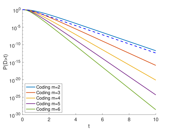
Figure 1: Complementary batch completition time distribution for a batch of $n=3$ jobs. The dashed line corresponds to replication with $d=3$ giving $nd$ replicated jobs, while the solid lines correspond to MDS with $n+m$ coded jobs.

Proof of Theorem 2. Equation (5) is a direct application of known results on order-statistics distributions. We now prove (4). Following derivations in [3, Section 5], denote by $T_{i}$ the non-redundant response time for a tagged job in queue $i$. Then

$$T_{i}=W_{i}+E_{i},$$

where $W_{i}$ is the workload (real workload, i.e. time to empty the queue if there were no more arrivals) and $E_{i}$ is an Exponential$(1)$ random variable (service requirement). Let us denote by $F_{T}$ and $F_{W}$ the distribution functions of $T$ and $W$, respectively. Let us also denote their tails by ${\overline{F}_{T}}$ and ${\overline{F}_{W}}$. Then we can write

$${\overline{F}_{T}}(t)=e^{-t}+\int_{0}^{t}e^{-y}{\overline{F}_{W}}(t-y)dy=e^{-t}+\int_{0}^{t}e^{-(t-y)}{\overline{F}_{W}}(y)dy=e^{-t}+e^{-t}\int_{0}^{t}e^{y}{\overline{F}_{W}}(y)dy,$$

differentiating which we get

$${\overline{F}_{T}}^{\prime}(t)={\overline{F}_{W}}(t)-{\overline{F}_{T}}(t).$$ (7)

Let us now write an expression for ${\overline{F}_{W}}(t)$. We can look at the previous arrival (which in the case of MDS happens an Exponential$(\lambda(m+n)/n)$ time earlier than the tagged arrival. For simplicity denote $\alpha=\lambda m/n$. Condition first on the previous arrival having been $y$ time before the tagged arrival. Then $W>t$ in one of two cases: either the previous arrival sees workload larger than $t+y$, or the previous arrival sees workload smaller than $t+y$, its own (non-redundant) time in queue $i$ is larger than $t+y$ and by the time $t+y$ no more than $n-1$ of the other $n+m-1$ copies left other queues (or, in other words, $n$th order statistic of $n+m-1$ random variables exceeds $t+y$);

Integrating over all values of $y$, we obtain:

$${\overline{F}_{W}}(t)=\int_{0}^{\infty}\alpha e^{-\alpha y}dy\biggl{(}{\overline{F}_{W}}(t+y)$$

$$+({\overline{F}_{T}}(t+y)-{\overline{F}_{W}}(t+y))(n+m-1){{n+m-2}\choose{n-1}}\sum_{i=0}^{n-1}{{n-1}\choose{i}}(-1)^{i}\frac{1}{m+i}({\overline{F}_{T}}(t+y))^{m+i}$$

$$=e^{\alpha t}\int_{t}^{\infty}\alpha e^{-\alpha z}dz\biggl{(}{\overline{F}_{W}}(z)$$

$$+({\overline{F}_{T}}(z)-{\overline{F}_{W}}(z))(n+m-1){{n+m-2}\choose{n-1}}\sum_{i=0}^{n-1}{{n-1}\choose{i}}(-1)^{i}\frac{1}{m+i}({\overline{F}_{T}}(z))^{m+i}\biggr{)},$$

where we used known results for the tail distribution of $n$th order statistic of $n+m-1$ random variables. Differentiating the above relation, we get

$${\overline{F}_{W}}^{\prime}(t) =\alpha{\overline{F}_{W}}(t)-\alpha\biggl{(}{\overline{F}_{W}}(t)$$

$$+(n+m-1){{n+m-2}\choose{n-1}}({\overline{F}_{T}}(t)-{\overline{F}_{W}}(t))\sum_{i=0}^{n-1}{{n-1}\choose{i}}(-1)^{i}\frac{1}{m+i}({\overline{F}_{T}}(t))^{m+i}\biggr{)}$$

$$=\alpha(n+m-1){{n+m-2}\choose{n-1}}{\overline{F}_{T}}^{\prime}(t)\sum_{i=0}^{n-1}{{n-1}\choose{i}}(-1)^{i}\frac{1}{m+i}({\overline{F}_{T}}(t))^{m+i},$$

where in the last equality we used (7). The above can be integrated and plugged into (7) to obtain

$${\overline{F}_{T}}^{\prime}(t)=-{\overline{F}_{T}}(t)+\alpha(n+m-1){{n+m-2}\choose{n-1}}\sum_{i=0}^{n-1}{{n-1}\choose{i}}(-1)^{i}\frac{1}{(m+i)(m+i+1)}({\overline{F}_{T}}(t))^{m+i+1}.$$

This proves (4). Recall that $m-n\geq 1$. Since ${\overline{F}_{T}}(x)\to 0$ as $x\to\infty$, there exists $X$ such that

$${\overline{F}_{T}}^{\prime}(x)\leq-{\overline{F}_{T}}(x)+A({\overline{F}_{T}}(x))^{2},$$

for all $x\geq X$, with some constant $A>0$. Denote by $g(x)=1/{\overline{F}_{T}}(x)$. Then

$$g^{\prime}(x)=-\frac{{\overline{F}_{T}}(x)}{({\overline{F}_{T}}(x))^{2}}\geq-\frac{-{\overline{F}_{T}}(x)+A({\overline{F}_{T}}(x))^{2}}{({\overline{F}_{T}}(x))^{2}}=g(x)-A$$

for all $x\geq X$. Since $g(x)\to\infty$ as $x\to\infty$, we can also assume that $g(x)\geq A$ for all $x\geq X$. Then the above implies that

$$\frac{g^{\prime}(x)}{g(x)-A}\geq 1$$

for all $x\geq X$. Integrating the above inequality from $X$ to $x$ implies

$$\log\left(\frac{g(x)-A}{g(X)-A}\right)\geq x-X,$$

and hence $g(x)\geq A+(g(X)-A)e^{x-X}\geq Be^{x}$, with a constant $B$. This of course implies (6), and the proof is complete. ∎

References

- [1] Y. Azar, A. Z. Broder, A. R. Karlin, and E. Upfal. Balanced allocations. SIAM journal on computing, 29(1):180–200, 1999.
- [2] L. Chen, H. Wang, Z. Charles, and D. Papailiopoulos. Draco: Byzantine-resilient distributed training via redundant gradients. Proceedings of Machine Learning Research, 80:903–912, 2018.
- [3] K. Gardner, M. Harchol-Balter, A. Scheller-Wolf, M. Velednitsky, and S. Zbarsky. Redundancy-d: The power of d choices for redundancy. Operations Research, 65(4):1078–1094, 2017.
- [4] K. Gardner, S. Zbarsky, S. Doroudi, M. Harchol-Balter, and E. Hyytia. Reducing latency via redundant requests: Exact analysis. ACM SIGMETRICS Performance Evaluation Review, 43(1):347–360, 2015.
- [5] W. Halbawi, N. Azizan, F. Salehi, and B. Hassibi. Improving distributed gradient descent using Reed-Solomon codes. In IEEE International Symposium on Information Theory, pages 2027–2031, 2018.
- [6] T. Hellemans, T. Bodas, and B. Van Houdt. Performance analysis of workload dependent load balancing policies. Proceedings of the ACM on Measurement and Analysis of Computing Systems, 3(2):35, 2019.
- [7] T. Ho, M. Médard, R. Koetter, D. R. Karger, M. Effros, J. Shi, and B. Leong. A random linear network coding approach to multicast. IEEE Transactions on Information Theory, 52(10):4413–4430, 2006.
- [8] L. Huang, S. Pawar, H. Zhang, and K. Ramchandran. Codes can reduce queueing delay in data centers. In IEEE International Symposium on Information Theory, pages 2766–2770, 2012.
- [9] G. Joshi, Y. Liu, and E. Soljanin. On the delay-storage trade-off in content download from coded distributed storage systems. IEEE Journal on Selected Areas in Communications, 32(5):989–997, 2014.
- [10] K. Lee, M. Lam, R. Pedarsani, D. Papailiopoulos, and K. Ramchandran. Speeding up distributed machine learning using codes. IEEE Transactions on Information Theory, 64(3):1514–1529, 2017.
- [11] K. Lee, N. B. Shah, L. Huang, and K. Ramchandran. The MDS queue: Analysing the latency performance of erasure codes. IEEE Transactions on Information Theory, 63(5):2822–2842, 2017.
- [12] B. Li, A. Ramamoorthy, and R. Srikant. Mean-field-analysis of coding versus replication in cloud storage systems. In IEEE International Conference on Computer Communications, pages 1–9. IEEE, 2016.
- [13] R. K. Maity, A. S. Rawat, and A. Mazumdar. Robust gradient descent via moment encoding with LDPC codes. In SysML Conference, 2019.
- [14] M. Mitzenmacher. The power of two choices in randomized load balancing. IEEE Transactions on Parallel and Distributed Systems, 12(10):1094–1104, 2001.
- [15] E. Ozfatura, D. Gunduz, and S. Ulukus. Gradient coding with clustering and multi-message communication. In IEEE Data Science Workshop, 2019.
- [16] E. Ozfaturay, D. Gunduz, and S. Ulukus. Speeding up distributed gradient descent by utilizing non-persistent stragglers. In IEEE International Symposium on Information Theory, 2019.
- [17] I. S. Reed and G. Solomon. Polynomial codes over certain finite fields. Journal of the society for industrial and applied mathematics, 8(2):300–304, 1960.
- [18] R. Roth. Introduction to coding theory. Cambridge University Press, 2006.
- [19] N. B. Shah, K. Lee, and K. Ramchandran. The mds queue: Analysing the latency performance of erasure codes. In 2014 IEEE International Symposium on Information Theory, pages 861–865. IEEE, 2014.
- [20] N. B. Shah, K. Lee, and K. Ramchandran. When do redundant requests reduce latency? IEEE Transactions on Communications, 64(2):715–722, 2015.
- [21] R. Tandon, Q. Lei, A. G. Dimakis, and N. Karampatziakis. Gradient coding: Avoiding stragglers in distributed learning. In International Conference on Machine Learning, pages 3368–3376, 2017.
- [22] M. van der Boor, S. C. Borst, J. S. van Leeuwaarden, and D. Mukherjee. Scalable load balancing in networked systems: A survey of recent advances. arXiv preprint arXiv:1806.05444, 2018.
- [23] N. D. Vvedenskaya, R. L. Dobrushin, and F. I. Karpelevich. Queueing system with selection of the shortest of two queues: An asymptotic approach. Problemy Peredachi Informatsii, 32(1):20–34, 1996.
- [24] L. Ying, R. Srikant, and X. Kang. The power of slightly more than one sample in randomized load balancing. Mathematics of Operations Research, 42(3):692–722, 2017.