Computational Phenotype Discovery
via Probabilistic Independence

Abstract.

Computational Phenotype Discovery research has taken various pragmatic approaches to disentangling phenotypes from the episodic observations in Electronic Health Records. In this work, we use transformation into continuous, longitudinal curves to abstract away the sparse irregularity of the data, and we introduce probabilistic independence as a guiding principle for disentangling phenotypes into patterns that may more closely match true pathophysiologic mechanisms. We use the identification of liver disease patterns that presage development of Hepatocellular Carcinoma as a proof-of-concept demonstration.

1. Introduction

There is growing evidence that insufficiently precise clinical diagnoses are responsible for a large fraction of current treatment failures (Anderson, 2008; Ringman et al., 2014; Gutmann, 2014; Tuomi et al., 2014). The goal of Computational Phenotype Discovery is to create a more precise set of patterns (or phenotypes) of clinically observable variables that better represent latent pathophysiologic mechanisms, and lead to more precise treatment decisions (Lasko et al., 2013).

Electronic Health Records (EHRs) are a popular substrate for phenotype discovery research, although the sparse, irregular, and asynchronous nature of the observations they contain is a well-known barrier to secondary use (Lasko et al., 2013; Lasko, 2013; Zhou et al., 2014; Ghassemi et al., 2015).

A useful mental model is to consider the observations in a patient’s record to have been placed there by noisy episodic processes run within each of the patient’s medical conditions. But because those conditions share a common vocabulary of observations, there is no obvious correspondence between the observed data and the unobserved conditions. The problem of disentangling the true latent processes from the sparse and irregularly observed data is the phenotype discovery problem.

This problem maps well to unsupervised feature learning, and several approaches have been taken to date. Some overcome sparsity and irregularity by aggregating counts of events within defined time windows, producing one learning instance per window. One line of research in this direction unraveled latent factors with Nonnegative Matrix Factorization (Ho et al., 2014). Another produced coarse phenotypes (on the granularity of ’Cardiovascular Disease’, or ’Lung Disease’) by decomposing the count matrix into a phenotype matrix and a densified temporal expression matrix, using constraints of smoothness, sparsity, and nonnegativity (Zhou et al., 2014). A more ambitious effort used stacked denoising autoencoders to decompose counts vectors for $700,000$ patients using a large set of counted events into a set of $500$ phenotypes (Miotto et al., 2016).

Other researchers have used dense time-series data from an Intensive Care Unit to avoid the episodic data problem. One group used denoising autoencoders as the decomposition method (Kale et al., 2015), and another cast the problem as a supervised multi-label problem, where clinical patterns were learned to predict the assignment of a particular billing code (Che et al., 2015).

In this work we make two contributions. First, we overcome the episodic data problem by transforming each sequence of repeated observations into a continuous longitudinal curve. We demonstrate this transformation on the two most common data types in an EHR. Second, we observe that while various methods have been used to disentangle the latent phenotypes from the original basis of observations, those methods appear to have been chosen from a pragmatic rather than a principled perspective. We propose using probabilistic independence as a principled choice for that disentanglement because it is more likely to illuminate actual disease mechanisms.

2. Methods

2.1. Data

All data for this project was extracted from the de-identified mirror of Vanderbilt’s Electronic Health Record, which contains administrative data, billing codes, medication exposures, laboratory test results, and narrative text for over 2 million patients, reaching back nearly 30 years (Roden et al., 2008). We obtained IRB approval to use the data in this research.

From this source, we extracted all ICD-9 billing codes and all results from the $500$ most common laboratory tests for all included records. We focused on patients with liver disease, although we expected phenotypes from the full range of conditions to appear among those patients. Inclusion criteria for a patient record were the presence of any lab result indicating at least mild liver disease (AST ¿ 40, ALT ¿ 55, or Alk Phos ¿ 150) or the presence of at least one ICD-9 billing code indicating Nonalcoholic Fatty Liver Disease (571.8, 571.9, or 571.5). This retrieved $259,000$ records, from which $30,000$ were sampled at random for tractability. The ICD-9 codes were grouped into $1,814$ Phecodes, for a total instance dimension of $2,314$ variables.

2.2. Longitudinal Curves

Previous work dealt with the episodic nature of medical data by aggregating that data into observation windows, with the instance vector containing the count of each variable’s event within that window. That approach has an inherent trade-off between statistical accuracy and window size. In contrast, we converted each observation sequence into a continuous longitudinal curve, for which any point on that curve estimates the instantaneous value for a given measure of a given variable at that point. The set of inferred curves can then be sampled at any desired point, giving dense cross sections to use for downstream learning. The semantics of each curve differ with the type of data it represents.

Longitudinal curves for ICD-9 codes represent the intensity function for a nonhomogeneous Gamma process over code-arrival events, and can be interpreted as the instantaneous event density in time (Lasko, 2014). This is a powerful representation that can account for burstiness, regularity, or randomness of event timing, and can provide uncertainty distributions for the inferred curves. Inferring a full model is computationally intensive, however, so for this work we used an approximate method that produces a similar intensity curve, but several orders of magnitude faster.

Longitudinal curves for laboratory test results represent a distribution of latent functions that could have produced the observed results. These were originally computed using nonstationary Gaussian process regression (Lasko, 2015). However, this inference is also computationally intensive, so we approximated it using a smooth interpolation algorithm that provides a similar mean curve, but without an uncertainty distribution, which is not necessary for this work.

Other data types could be similarly represented by continuous curves, but these two are the canonical types covering most of the structured data in a patient record: event data with times and variable labels but no values, and measurement data with times, variable labels, and measured values.

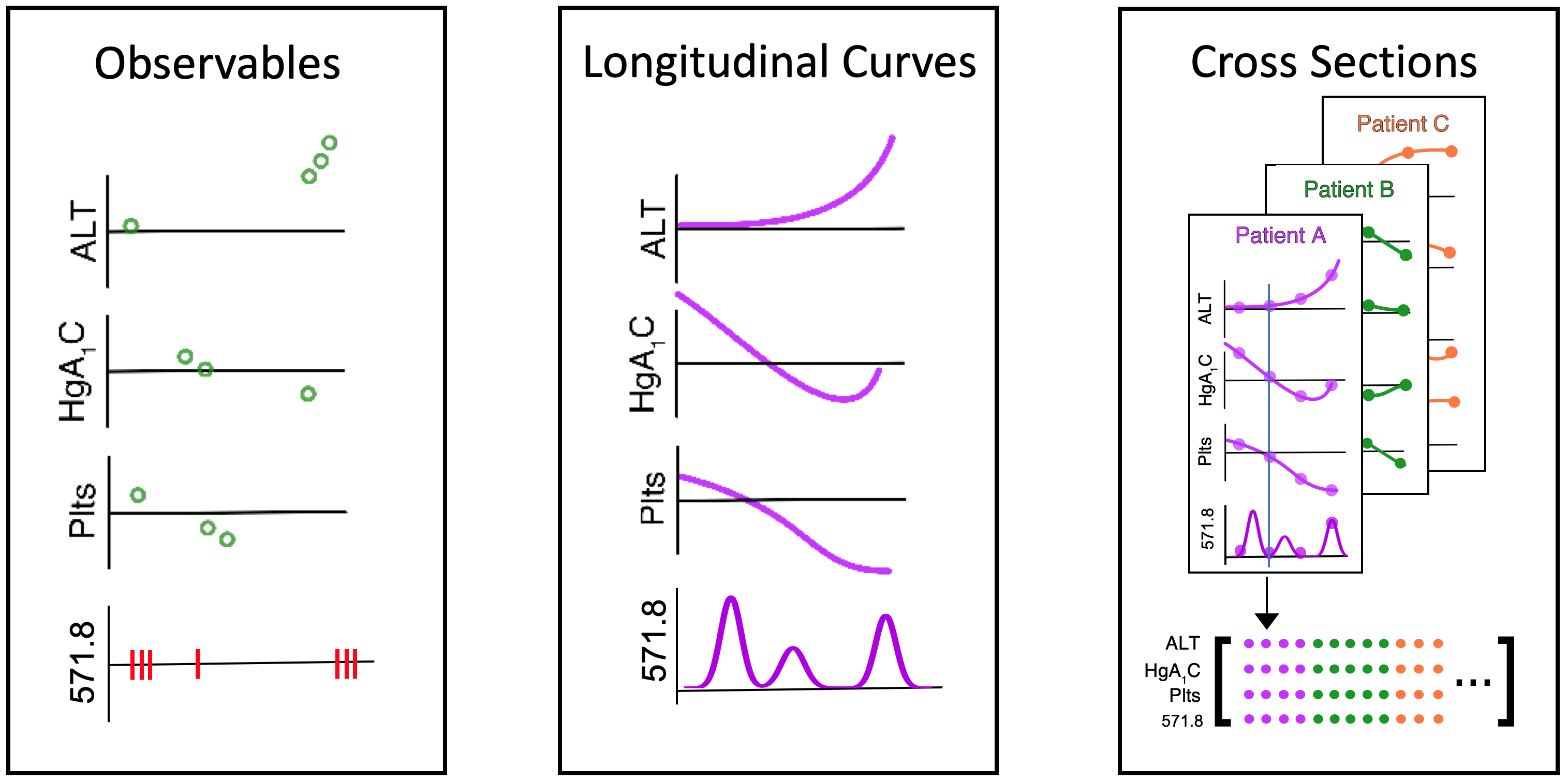
Figure 1. Preprocessing steps to produce the input dataset. Episodic data observations (left) are converted into continuous longitudinal curves (middle), which are then sampled at random points to produce cross sections (right), which form the dense data matrix (bottom right).

[¡short description¿]¡long description¿

2.3. Independence

Our second contribution is the use of probabilistic independence as a principled means for disentangling clinical phenotypes. Our underlying hypothesis is that distinct pathophysiologic processes operate independently from each other, and as such would leave probabilistically independent phenotypic fingerprints in the record.

Independence has previously been proposed as a principle for disentangling factors of variation in deep architectures (Chen et al., 2018; Li et al., 2019), but to our knowledge it has not been described as a guiding principle for phenotype discovery. We anticipate that deep architectures using this principle will eventually become the dominant approach to phenotype discovery, but we do not use them in this work, because if nothing else, the discovered phenotypes would be difficult to unambiguously visualize and evaluate.

We chose Independent Components Analysis (ICA) (Hyvarinen et al., 2001) as an approach that isolates the principle of independence for disentangling phenotypes and provides a linear decomposition that is easy to directly visualize. ICA also makes the assumption that phenotype compositions are constant in time (although the level expressed by a given patient may change with time). This is a useful simplification but not required by the domain problem.

One instance of prior work does use ICA in passing as an un-optimized baseline comparison, but does not directly evaluate the phenotypes produced (Miotto et al., 2016).

2.4. Experiment Details

Records were extracted from the data source as described, and curves were computed for each of the $n=2,314$ variables for each patient, for the duration of each record. ICD-9 codes that did not occur in the record produced a constant curve of zero intensity. Lab results that did not occur in the record were filled a constant curve with the population median value. Cross sections of each record’s curve sets were then sampled at specific points in time chosen uniformly at random at an average density of $1$ sample per year, giving $m=180,369$ total instances (Fig. 1).

This dataset $X\in\mathbb{R}^{n\times m}$ was then decomposed by ICA into $X=AS$, where the phenotypic patterns of interest appeared in the columns of $A$, and the patient-specific expression levels appeared in the rows of $S$. We arbitrarily set the dimension of the phenotype space (the rank of $A$ and $S$) to $500$.

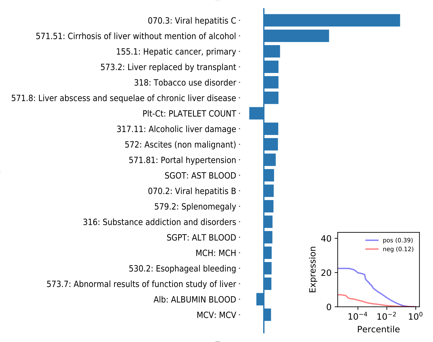
(a) Late Hepatitis C

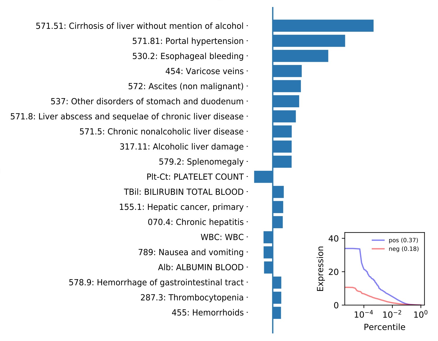
(b) Early Nonalcoholic Cirrhosis

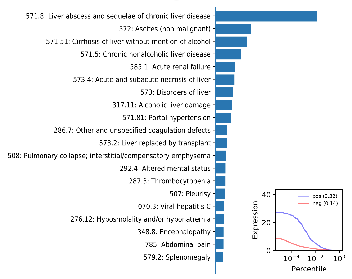
(c) Late Nonalcoholic Cirrhosis

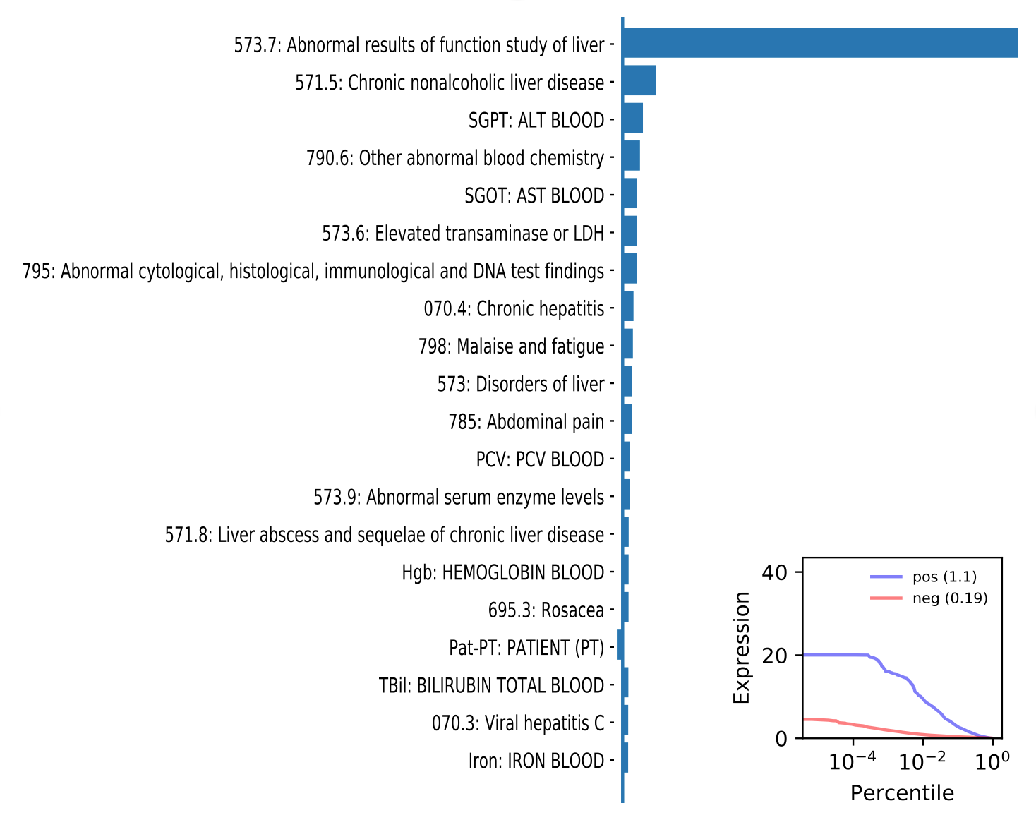
(d) Mild Non-alcoholic Steatohepatitis

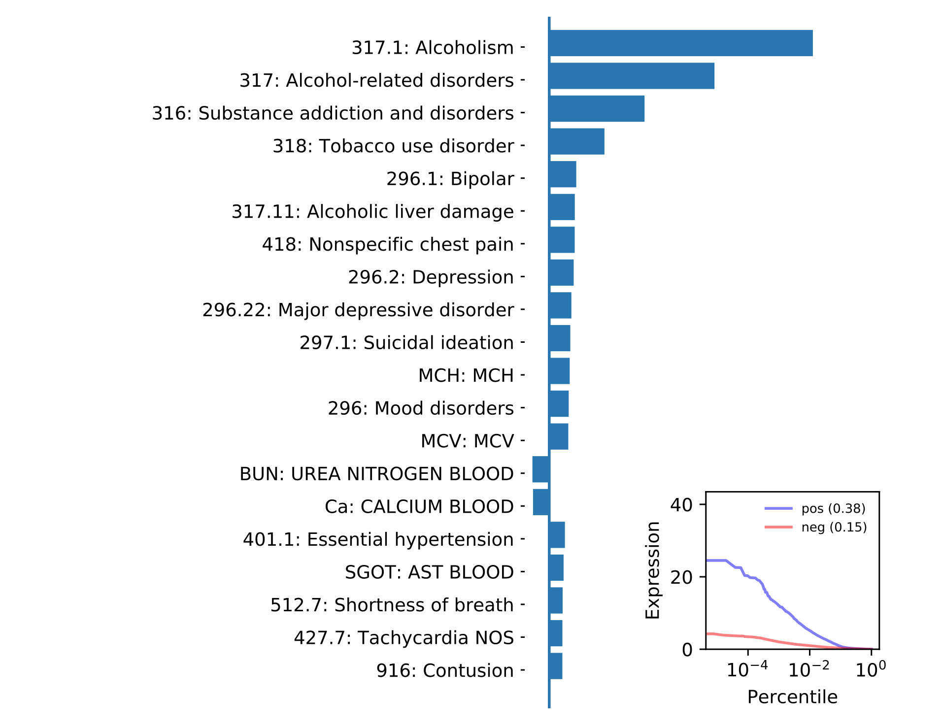
(e) Alcohol Dependence

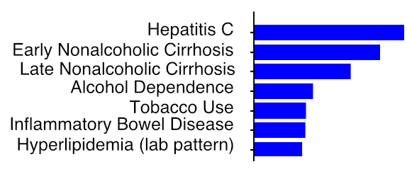
(f) HCC Precursors

Figure 2. Data-driven phenotypes include surprisingly detailed distinctions between early and late disease (a through e), and identify patterns that presage Hepatocellular Carcinoma (HCC) by 10 years (f). The disease name in each caption was assigned by an expert, not by the algorithm.

[¡short description¿]¡long description¿

2.5. Evaluation

The resulting phenotypes were evaluated in two ways: first, using clinical face validity as judged by a domain expert, and second, by using them to investigate conditions that presage the diagnosis of Hepatocellular Carcinoma (HCC, a type of liver cancer).

The HCC investigation was formulated as a learning problem that predicts the presence of an HCC billing code in the record exactly $10$ years from the time of the cross section, given that there is no such code before then. This is different from (and harder than) the usual risk prediction problem, where the goal would be to predict whether the event will occur any time over the next $10$ years.

Our formulation allows us to examine the cancer disease process in terms of our phenotypes a decade before its diagnosis. The salient piece of the results (given adequate prediction accuracy) is an examination of the phenotypes that are important to the prediction, and a judgment of whether they align with what is known about the pathophysiology of HCC, and whether the results suggest anything new about the disease.

We constructed negative instances from all records at least $10$ years long that did not have an HCC diagnosis code ($155.0$, $155.1$, or $155.2$), and positive instances from all those with at least $10$ years before the earliest HCC code. Records with fewer than $10$ pieces of data distributed among all ICD codes and lab values were excluded. This produced $l=40,398$ instances, of which $197$ were positive. We formed the raw data matrix $X\in\mathbb{R}^{n\times l}$ as above, and then projected it into phenotype space using $S=A^{-1}X$. A random forest was trained on the phenotype expression matrix $S$ to predict the disease label.

3. Results

The subjective evaluation of phenotype face validity was promising. About $80-90\%$ of the discovered phenotypes were clearly recognizable as a specific disease pattern. Among these were several phenotypes of mild to severe liver disease at a surprisingly high level of differentiation (Fig. 2(f)), such as very mild disease with only slight changes in liver enzymes (panel d), early vs. late nonalcoholic cirrhosis patterns (panels b and c), late-stage Hepatitis C (panel a), and alcohol dependence (panel e). Of the non-recognizable phenotypes (not shown, for space) many described complex laboratory result patterns with some underlying theme, but which did not immediately suggest an obvious disease. We interpret these phenotypes as a positive result, because they suggest laboratory patterns that may correspond to specific disease mechanisms, but which have not yet been recognized, so there are no billing codes for them.

The prediction model produced an adequate $0.76$ AUC, within the range of historical results on the harder risk prediction problem. The phenotype forerunners of HCC, identified using the feature importance measure, are also very satisfying. The conditions in our list are known to eventually produce the tumor-generating environment needed for HCC, and their order here matches known risk factors in the US (Ma et al., 2016). They also match exactly, and in order, the top causes of liver transplant, which is the definitive treatment of HCC (Wong et al., 2015). The next three phenotypes suggest interesting mechanisms that reflect known or suspected risk factors (Ma et al., 2016; Koh et al., 2011; Rojas-Feria et al., 2013; Ioannou, 2016).

4. Discussion

This work introduces the use of independence for disentangling latent phenotypes from EHR data, and it demonstrates the transformation of episodic clinical data into continuous longitudinal curves to overcome well-known hurdles to learning from that data.

Our approach learned $500$ different clinical patterns of billing codes and laboratory values. These patterns provide a surprisingly granular set of phenotypes that match clinical intuition, describing some conditions at multiple stages, including subtle patterns of mild disease as well as obvious patterns of severe disease. It is straightforward to extend the input data to include other data types such as medications, demographics, and concepts in the text.

A predictive model used the learned phenotypes to identify a small set of conditions that presage liver cancer by $10$ years, recovering known precursors of that disease and strengthening previous suggestions about additional risk factors. These findings suggest (but do not prove) a reasonable correspondence to pathophysiologic mechanisms.

The number of phenotypes and the size of the input dataset are limited by available memory under ICA decomposition, but are expandable by orders of magnitude using deep architectures with suitable constraints to provide independence. Deep architectures would also provide nonlinear decompositions, but they would be more challenging to visualize and evaluate.

The best way of meaningfully evaluating the match between a set of data-driven phenotypes and true pathophysiologic processes is currently an open question. Previous work has commonly evaluated a set of phenotypes by their performance in a clinical prediction model. We reject that approach because it doesn’t measure the most important property, which is how faithfully the phenotypes represent actual disease mechanisms. Deep prediction model performance is a particularly deceptive measure, because deep models are capable of making excellent predictions from many different input representations, so long as those representations somehow include sufficient information for the prediction.

In light of that open question, we evaluated our phenotypes using subjective methods that try to assess how well the learned phenotypes correspond to what is known about an a-priori selected disease process, and whether they point us in interesting clinical research directions. On both of these questions, our learned phenotypes were quite promising.

References

- (1)
- Anderson (2008) Gary P. Anderson. 2008. Endotyping asthma: new insights into key pathogenic mechanisms in a complex, heterogeneous disease. Lancet 372, 9643 (Sep 2008), 1107–1119.
- Che et al. (2015) Zhengpoing Che, David Kale, Wenzhe Li, Mohammad Taha Bahadori, and Yan Liu. 2015. Deep Computational Phenotyping. In Proceedings of the 21th ACM SIGKDD International Conference on Knowledge Discovery and Data Mining (KDD’15).
- Chen et al. (2018) Tian Qi Chen, Xuechen Li, Roger B Grosse, and David K Duvenaud. 2018. Isolating sources of disentanglement in variational autoencoders. In NIPS 2018. 2610–2620.
- Ghassemi et al. (2015) Marzyeh Ghassemi, Marco A F Pimentel, Tristan Naumann, Thomas Brennan, David A Clifton, Peter Szolovits, and Mengling Feng. 2015. A Multivariate Timeseries Modeling Approach to Severity of Illness Assessment and Forecasting in ICU with Sparse, Heterogeneous Clinical Data. AAAI 2015 2015 (Jan. 2015), 446–453.
- Gutmann (2014) David H. Gutmann. 2014. Eliminating barriers to personalized medicine: Learning from neurofibromatosis type 1. Neurology (Jun 2014).
- Ho et al. (2014) Joyce C. Ho, Joydeep Ghosh, and Jimeng Sun. 2014. Marble: High-throughput Phenotyping from Electronic Health Records via Sparse Nonnegative Tensor Factorization. In KDD 2014 (KDD ’14). ACM, New York, NY, USA, 115–124.
- Hyvarinen et al. (2001) Aapo Hyvarinen, Juha Karhunen, and Erkki Oja. 2001. Independent Component Analysis. Wiley, New York.
- Ioannou (2016) George N Ioannou. 2016. The Role of Cholesterol in the Pathogenesis of NASH. Trends Endocrinol Metab 27 (Feb. 2016), 84–95. Issue 2.
- Kale et al. (2015) David C. Kale, Zhengping Che, Mohammad Taha Bahadori, Wenzhe Li, Yan Liu, and Randall Wetzel. 2015. Causal Phenotype Discovery via Deep Networks. In Proceedings AMIA Symposium 2015.
- Koh et al. (2011) W-P Koh, K Robien, R Wang, S Govindarajan, J-M Yuan, and M C Yu. 2011. Smoking as an independent risk factor for hepatocellular carcinoma: the Singapore Chinese Health Study. Br J Cancer 105 (Oct. 2011), 1430–1435. Issue 9.
- Lasko (2013) Thomas A Lasko. 2013. Inferring the Latent Intensity of Clinical Events Using Modulated Renewal Processes. In NIPS 2013 Workshop on Machine Learning for Clinical Data Analysis and Healthcare.
- Lasko (2014) Thomas A. Lasko. 2014. Efficient Inference of Gaussian Process Modulated Renewal Processes with Application to Medical Event Data. In Proceedings of the Thirtieth Conference on Uncertainty in Artificial Intelligence (UAI). arXiv:1402.4732
- Lasko (2015) Thomas A Lasko. 2015. Nonstationary Gaussian Process Regression for Evaluating Clinical Laboratory Test Sampling Strategies. AAAI 2015 (Jan 2015), 1777–1783.
- Lasko et al. (2013) Thomas A. Lasko, Joshua C. Denny, and Mia A. Levy. 2013. Computational Phenotype Discovery Using Unsupervised Feature Learning over Noisy, Sparse, and Irregular Clinical Data. PLoS One 8, 6 (2013), e66341.
- Li et al. (2019) Yang Li, Quan Pan, Suhang Wang, Haiyun Peng, Tao Yang, and Erik Cambria. 2019. Disentangled variational auto-encoder for semi-supervised learning. Information Sciences 482 (2019), 73–85.
- Ma et al. (2016) Xiao Ma, Yang Yang, Hong Tu, Jing Gao, Yu-Ting Tan, Jia-Li Zheng, Freddie Bray, and Yong-Bing Xiang. 2016. Risk prediction models for hepatocellular carcinoma in different populations. Chin J Cancer Res 28 (April 2016), 150–160. Issue 2.
- Miotto et al. (2016) Riccardo Miotto, Li Li, Brian A. Kidd, and Joel T. Dudley. 2016. Deep Patient: An Unsupervised Representation to Predict the Future of Patients from the Electronic Health Records. Sci Rep 6 (2016), 26094.
- Ringman et al. (2014) JohnM. Ringman, Alison Goate, ColinL. Masters, NigelJ. Cairns, Adrian Danek, Neill Graff-Radford, Bernardino Ghetti, and JohnC. Morris. 2014. Genetic Heterogeneity in Alzheimer Disease and Implications for Treatment Strategies. Curr Neurol Neurosci Rep 14, 11, Article 499 (2014).
- Roden et al. (2008) D. M. Roden, J. M. Pulley, M. A. Basford, G. R. Bernard, E. W. Clayton, J. R. Balser, and D. R. Masys. 2008. Development of a large-scale de-identified DNA biobank to enable personalized medicine. Clin Pharmacol Ther 84, 3 (Sep 2008), 362–369.
- Rojas-Feria et al. (2013) María Rojas-Feria, Manuel Castro, Emilio Suárez, Javier Ampuero, and Manuel Romero-Gómez. 2013. Hepatobiliary manifestations in inflammatory bowel disease: the gut, the drugs and the liver. World J Gastroenterol 19 (Nov. 2013), 7327–7340. Issue 42.
- Tuomi et al. (2014) Tiinamaija Tuomi, Nicola Santoro, Sonia Caprio, Mengyin Cai, Jianping Weng, and Leif Groop. 2014. The many faces of diabetes: a disease with increasing heterogeneity. Lancet 383, 9922 (2014), 1084–1094.
- Wong et al. (2015) Robert J Wong, Maria Aguilar, Ramsey Cheung, Ryan B Perumpail, Stephen A Harrison, Zobair M Younossi, and Aijaz Ahmed. 2015. Nonalcoholic steatohepatitis is the second leading etiology of liver disease among adults awaiting liver transplantation in the United States. Gastroenterology 148 (March 2015), 547–555. Issue 3.
- Zhou et al. (2014) Jiayu Zhou, Fei Wang, Jianying Hu, and Jieping Ye. 2014. From Micro to Macro: Data Driven Phenotyping by Densification of Longitudinal Electronic Medical Records. In KDD 2014 (KDD ’14). ACM, New York, NY, USA, 135–144.