Generalized Aubry-André-Harper model with modulated hopping and $p$-wave pairing

Abstract

We study an extended Aubry-André-Harper model with simultaneous modulation of hopping, on-site potential, and $p$-wave superconducting pairing. For the case of commensurate modulation of $\beta=1/2$ it is shown that the model hosts four different types of topological states: adiabatic cycles can be defined which pump particles, two types of Majorana fermions, or Cooper pairs. In the incommensurate case we calculate the phase diagram of the model in several regions. We characterize the phases by calculating the mean inverse participation ratio and perform multi-fractal analysis. In addition, we characterize whether the phases found are topologically trivial or not. We find an interesting critical extended phase when incommensurate hopping modulation is present. The rise between the inverse participation ratio in regions separating localized and extended states is gradual, rather than sharp. When, in addition, the on-site potential modulation is incommensurate, we find several sharp rises and falls in the inverse participation ratio. In these two cases all different phases exhibit topological edge states. For the commensurate case we calculate the evolution of the Hofstadter butterfly and the band Chern numbers upon variation of the pairing parameter for zero and finite on-site potential. For zero on-site potential the butterflies are triangular-like near zero pairing, when gap-closure occurs, they are square-like, and hexagonal-like for larger pairing, but with the Chern numbers switched compared to the triangular case. For the finite case gaps at quarter and three-quarters filling close and lead to a switch in Chern numbers.

I Introduction

The physics of Anderson delocalization-localization (or metal-insulator) transition in disordered fermionic systems is a problem of long-standing interest in condensed matter physics Anderson58 ; Evers08 ; Abrahams2010 . In one dimension uncorrelated random potentials lead to complete localization of all eigenfunctions Shima04 ; Izrailev12 , while mobility edges and the delocalization-localization transition will typically appear in 3D disordered systems. However, mobility edges may occur in some 1D systems Biddle11 ; Zhang15arXiv ; Wang17 , if the disorder distribution is deterministic, rather than uncorrelated. The paradigm of this class of quasi-periodic systems, incommensurate lattices (the superposition of two periodic lattices with incommensurate periods) is the Aubry-André model AA80 , or its two-dimensional analog, the Harper Harper55 model. The delocalization-localization transition due to the disordered on-site potential can appear in the Aubry-André model when the lattice is incommensurate, arising from the self-duality of this model Aulbach04 .

The model was explored AA-Top1 ; AA-Top2 ; AA-Top3 from a topological perspective. In the Aubry-André model with $p$-wave superconducting (SC) pairing the connection between the Su–Schrieffer–Heeger-like Su79 and the Kitaev-like Wakatsuki14 ; Kitaev01 topological phases was investigated Zeng16 . Other studies Thouless88 ; Sarma88 ; Sarma10 ; Liu18 focused on localization effects. In addition, commensurate and incommensurate modulations may appear in on-site and hopping terms, the interplay between the two was studied in Ref.  Cestari16, . When hopping modulations are incommensurate, Liu15 the system will go through Anderson-like localization, but no mobility edge is found. For commensurate hopping modulations topological zero-energy edge modes are found Liu15 ; Ganeshan13 . In Ref.  Cestari16, the incommensurate and commensurate off-diagonal modulations were combined resulting in the conclusion that the states depend on the phase between the two. Experimentally the model was realized in ultracold atoms in optical lattices Chabe ; Roati08 and in photonic crystals Negro03 ; Lahini09 . A recent experiment Kraus12 , realized the topological edge state.

In this paper, we study a generalized AAH model with modulated on-site potential, hopping, and $p$-wave pairing. For the bi-partite case ($\beta=1/2$) we show that four different topological excitations are possible. The same model, but without modulation of the $p$-wave pairing was studied by Zeng et al. Zeng16 and Liu et al. Liu18 . They studied both the commensurate and incommensurate cases. They mapped the phase diagram of the model, studied localization by investigating the mean inverse participation ratio (MIPR), and did multi-fractal analysis in the incommensurate case and showed the existence of topological edge states in the commensurate case. We also do these calculations for the model with modulated $p$-wave pairing. The MIPR studies of the critical extended phases give an interesting result. When incommensurate hopping modulation is turned on we see a “smeared mobility edge” phase, in which the rise in the MIPR between the localized and extended regions is gradual, rather than sharp. (Fig. 7). Other GAAHs all show a sharp jump Sarma10 ; Liu15 in mobility edge phases. When, in addition, incommensurate on-site potential modulation is turned on, the rise in MIPR between localized and extended regions are sharp again, but there are more than one such jumps in MIPR. In these last two incommensurate studies topological edge states exist in all phases. Also, for the commensurate lattice, we investigate the Chern numbers of the main gaps during the change of the modulated $p$-wave SC pairing strength. We find that values of the Chern numbers are changing with and without on-site potential when we tune the modulated $p$-wave SC pairing strength. The modulated $p$-wave pairing strength changes, the energy spectrum alters from the triangular-lattice like Hofstadter butterfly to one which is square-lattice like.

Our paper is organized as follows: In the next section (Sec. II), the generalized version of the GAAH model that includes nearest-neighbor and next-nearest-neighbor $p$-wave SC pairing is defined on the infinite lattice. In Sec. III, we extend the 1D model to an “ancestor” 2D $p$-wave SC model. In Sec. IV, we check topological properties of the pure commensurate lattice for the $\beta={1/2}$. In Sec. V, we consider the incommensurate modulations case for $\beta$, where we will discuss the metal-insulator transition, and especially the influences of the modulated $p$-wave SC pairing strength on this transition. In Sec. VI, for pure commensurate lattice, the corresponding Hofstadter butterflies are discussed in detail. We conclude the paper in Sec. VII.

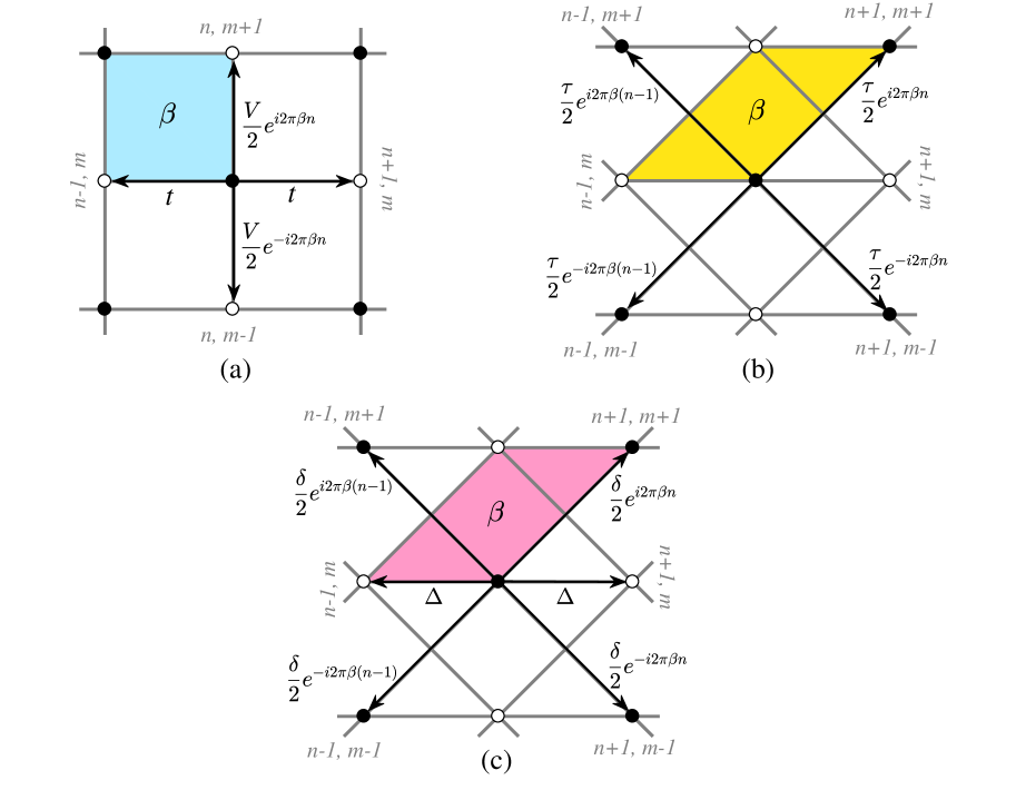
Figure 1: Graphical presentations of extended 1d GAAH with nearest and next-nearest hopping (SC pairing) and on-site potential to a 2D Hamiltonian. In the presence of a perpendicular magnetic field with $\beta$ flux quanta per unit cell, the electrons hop on a rectangular lattice. (a) This is the 2D “ancestor” of the diagonal GAAH model which the hopping is to nearest neighbors, (b) This is the 2D “ancestor” of the off-diagonal GAAH model which the hopping is to next-nearest neighbors, and (c) This is the 2D “ancestor” of the SC pairing of GAAH model which the hopping is to nearest and next nearest neighbors. Each rectangular plaquettes shown in different colors are pierced by $\beta$ flux quanta.

II The Model

The generalized one-dimensional Aubry-André-Harper model with $p$-wave SC pairing which we study here is described by the following Hamiltonian

$$\begin{split}\hat{{H}}&=-\sum_{j}\left[(t+\tau_{j})c_{j}^{\dagger}c_{j+1}+\mbox{H.c.})\right]\\ &\;\;\;\;+\sum_{j}(\Delta+\delta_{j})c_{j}^{\dagger}c_{j+1}^{\dagger}+\mbox{H.c.})+\sum_{j}V_{j}\hat{n}_{j}\end{split}$$ (1)

where

$$\begin{cases}\tau_{j}=\tau\cos(2\pi\beta j+\phi_{\tau}),\\ \delta_{j}=\delta\cos(2\pi\gamma j+\phi_{\delta}),\\ V_{j}=V\cos(2\pi\beta j+\phi_{V}).\end{cases}$$ (2)

Here $\tau_{j}$ is commensurate (incommensurate) hopping modulations with periodicity $1/\beta$ and phase factor $\phi_{\tau}$, and $V_{j}$ is the diagonal Aubry-André potential with periodicity $1/\beta$ and phase factor $\phi_{V}$, respectively. The corresponding hopping modulation amplitude is set by $\tau$, and $V$ is the on-site potential strength. $\hat{n}_{j}=c_{j}^{\dagger}c_{j}$ are number operators, $c_{j}^{\dagger}$($c_{j}$) are creation (annihilation operators) at position $j$ on the lattice, and $t$ is the hopping (or tunneling) amplitudes to the nearest neighbors and set to be the unit of the energy ($t=1$). Also, $\delta_{j}$ is a SC modulation with periodicity $1/\beta$ and phase factor $\phi_{\delta}$. Here $\delta$ and $\Delta$ are the strengths of SC pairing gap taken to be real.

In the limit $\Delta=\delta=0$, this model reduces to the generalized Aubry-André-Harper model introduced by Ganeshan et al. (Ganeshan13, ). If $\delta=0$ and $\phi_{\tau}=\phi_{V}$, this model reduces to the GAAH model with $p$-wave SC pairing introduced in Ref. Zeng16 and studied in Ref.  Liu18 . If we set $\tau=\delta=0$ the model exhibits an Anderson localization transition when $V>2(t+\Delta)$ Cai13 . On the other hand, if $\Delta$, and $\delta$ are zero, but $\tau$ and $V$ are finite, and when the relation between the hopping modulation and on-site phases are fixed, for example, $\phi_{V}=\phi_{\tau}+\beta\pi$, the GAA model can be formally derived from an ancestor 2D quantum Hall system on a lattice (Hofstadter model) with diagonal (next-nearest-neighbor) hopping terms Hiramoto89 ; Han94 ; Kraus12 . Here we keep our notations general with $\phi_{\tau}=\phi_{\delta}=k_{y}$ and $\phi_{V}=k_{y}+\varphi$ as independent variables. The off-diagonal modulation has an additional phase $\varphi$.

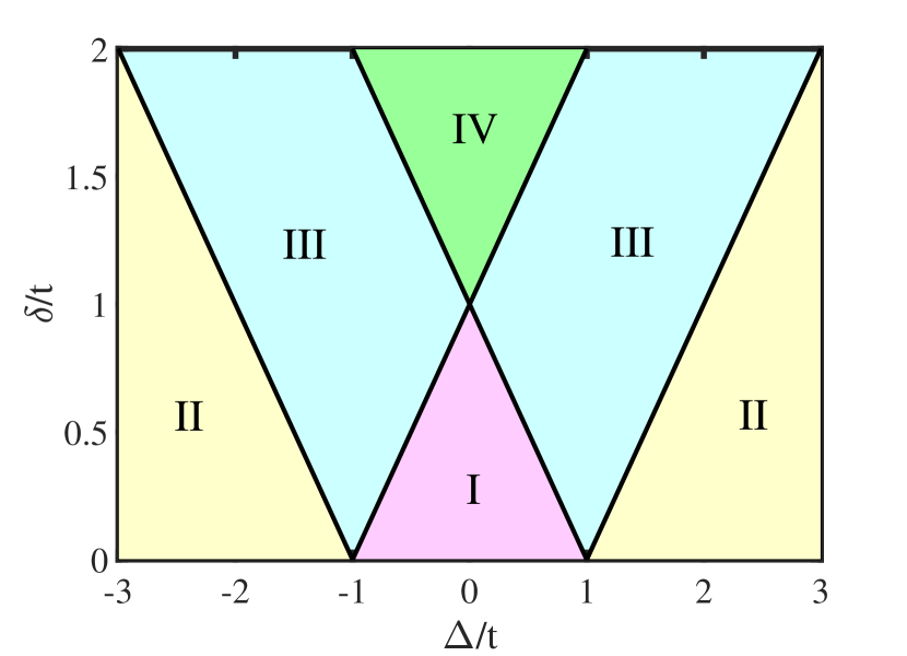
Figure 2: Phase diagram of the off-diagonal GAAH model as a function of the $p$-wave incommensurate modulation amplitude $\delta$ and the $p$-wave pairing strength $\Delta$. The hopping incommensurate modulation amplitude is set to $\tau=0$ and the phase in the incommensurate modulation is set to $k_{y}=\pi/2$ and $\varphi=\beta\pi$. The phases are (I and II) extended phases, (III) topological critical phase, and (IV) non-topological critical phase.

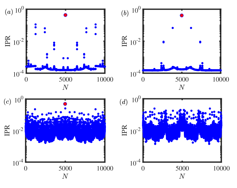
Figure 3: (Color online) The distribution of IPRs over all the eigenstates for (a) and (b) extended phases, (c) topological critical phase, and (d) non-topological critical phase of Fig. 2.

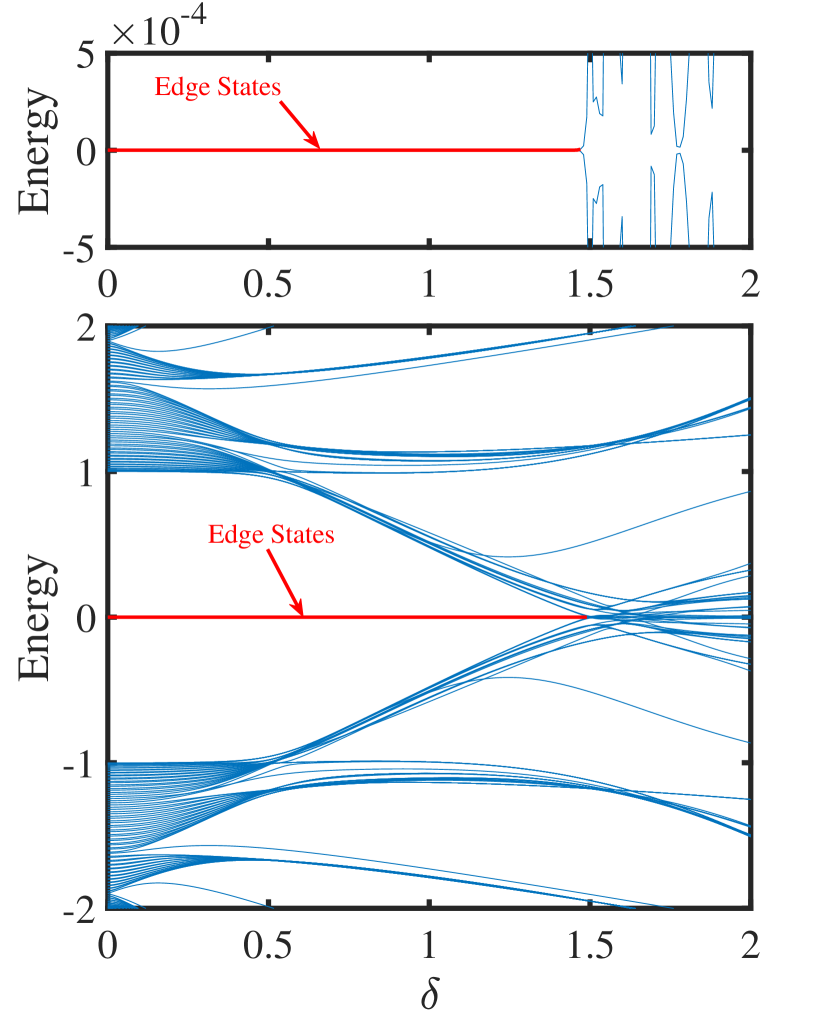
Figure 4: The energy spectrum of the off-diagonal GAAH model with $p$-wave pairing plotted as a function of $\delta$ under OBCs with $L=100$ lattice sites. The model parameters are $\tau=0$, $V=0$, and $\Delta=0.5$. Inside the regions I and II (see figure 2) there are edge states.

III The 2D analog of the generalized Aubry-André model with $p$-wave superconductivity

The Hamiltonian of the 1D GAAH model with $p$-wave superfluid pairing we consider in this paper can be made to correspond to a 2D $p$-wave SC model. For any given $k_{y}$, the GAAH model of Eq. (1) can be viewed as the $k_{y}$th Fourier component of a general 2D Hamiltonian. On the other hand, $k_{y}$ is the second degree of freedom, hence, we define the operator $c_{n,k_{y}}$ that satisfies the following commutation relation

$$\{c_{n,k_{y}},c^{\dagger}_{\acute{n},\acute{k_{y}}}\}=\delta_{n,\acute{n}}\delta_{k_{y},\acute{k_{y}}}$$ (3)

Therefore the 2D Hamiltonian can be expressed in terms of $\hat{H}$ as

$$\hat{\mathcal{H}}=\frac{1}{2\pi}\int_{0}^{2\pi}\hat{H}(k_{y})\;dk_{y}$$ (4)

where in the Hamiltonian of Eq. (1), we replaced the operators $c_{n}$ with $c_{n,k_{y}}$. The corresponding Hamiltonian can be written as

$$\begin{split}\hat{H}(k_{y})&=-\sum_{n}\left[(t+\tau_{n})c_{n,k_{y}}^{\dagger}c_{n+1,k_{y}}+\mbox{H.c.}\right]\\ &\;\;\;\;+\sum_{n}\left[(\Delta+\delta_{n})c_{n,k_{y}}^{\dagger}c_{n+1,-k_{y}}^{\dagger}+\mbox{H.c.})\right]\\ &\;\;\;\;+\sum_{n}V_{n}c_{n,k_{y}}^{\dagger}c_{n,k_{y}}\end{split}$$ (5)

Fourier transforming only in the $y$-direction

$$c_{n,k_{y}}=\sum_{m}e^{-ik_{y}m}c_{n,m}$$ (6)

allows us to easily calculate the 2D Hamiltonian as

$$\begin{split}\hat{\mathcal{H}}&=\sum_{n,m}-\left\{tc_{n,m}^{\dagger}c_{n+1,m}\right.\\ &-\left[\frac{\tau}{2}\left((e^{i2\pi\beta n}c_{n,m}^{\dagger}c_{n+1,m+1}+e^{-i2\pi\beta n}c_{n,m}^{\dagger}c_{n+1,m-1}\right)\right]\\ &+\left[\frac{\delta}{2}\left(e^{i2\pi\beta n}c_{n,m}^{\dagger}c^{\dagger}_{n+1,m+1}+e^{-i2\pi\beta n}c_{n,m}^{\dagger}c^{\dagger}_{n+1,m-1}\right)\right.\\ &\left.+\Delta c_{n,m}c_{n+1,m}\right]+\frac{V}{2}e^{i(2\pi\beta n+\varphi)}c_{n,m}^{\dagger}c_{n,m+1}\left.+\mbox{H.c.}\right\}.\end{split}$$ (7)

When $\varphi=0$, the 2D system has isotropic next-nearest-neighbor hoppings and the corresponding 1D Hamiltonian has the same phase $k_{y}$ in the off-diagonal and diagonal modulations. This Hamiltonian describes a 2D lattice in the presence of a uniform perpendicular magnetic field with $\beta$ flux quanta per unit cell as shown in Fig. 1.

IV Commensurate modulation, the case of $\beta=\frac{1}{2}$

Setting $\beta=\frac{1}{2}$ in Eq. (1), and all three phases to zero, the lattice becomes bi-partite. Introducing the notation $c_{i}$ and $d_{i}$ for the two sublattices, Fourier transforming using the Nambu basis ${c_{k}^{\dagger},d_{k}^{\dagger},c_{-k},d_{-k}}$, the Hamiltonian becomes

$$\hat{{H}}=-2t\cos(k)\sigma_{z}\otimes\sigma_{x}-2\tau\sin(k)\sigma_{z}\otimes\sigma_{y}\hskip 7.22743pt$$ (8)

$$+V\sigma_{z}\otimes\sigma_{z}-2\Delta\sin(k)\sigma_{y}\otimes\sigma_{x}+2\delta\cos(k)\sigma_{y}\otimes\sigma_{y}.$$

Note that the first three terms correspond to $\sigma_{z}\otimes\hat{{H}}_{RM}$, where $\hat{{H}}_{RM}$ is the Rice-Mele Hamiltonian. It follows that if we set $\Delta=\delta=V=0$ the model consists of two independent SSH models (which are topological), and it is possible to define an adiabatic process in which charge is pumped across the unit cell (the topological edge states support charges localized at the edges of the system). In a similar vein, keeping $V=0$, it is possible to pair the two $\cos(k)$ with the two $\sin(k)$ terms in four ways. Keeping the other parameters zero leads to other possible topological states, or possible adiabatic pumping processes. Of the remaining three, two are Majorana fermions, and the fourth one a Cooper pair. For example, we can take $\tau=\delta=0$ resulting in

$$\hat{{H}}=[-2t\cos(k)\sigma_{z}-2\Delta\sin(k)\sigma_{y}]\otimes\sigma_{x},$$ (9)

in other words, a $2\times 2$ Hamiltonian of the SSH form, but the adiabatic pumping in this case would not correspond to a charge pump, because different members of the Nambu bases are coupled by the matrix elements. For each of the four cases it is possible to construct the time-reversal, particle-hole symmetry operators, as well as the chiral symmetry operators using the “left” or the “right” part of the direct product and multiplying with an identity operator from the other side. They all fall in the BDI symmetry class Altland97 .

V Incommensurate modulation

When $\beta$ is irrational, the lattice is incommensurate. We choose $\beta=(\sqrt{5}-1)/2$, the golden ratio, but all the conclusions can also be generalized to other incommensurate situations. In this paper, for incommensurate modulation case, we shall study the interplay of the SC modulation pairing $\delta$ with the incommensurate hopping amplitude and potential, respectively, and then we determine the phase diagram of the model. The Hamiltonian can be diagonalized by the Bogoliubov–de Gennes (BdG) transformation Lieb61 ; Gennes66

$$\eta_{n}^{\dagger}=\sum_{j=1}^{L}[u_{n,j}c_{j}^{\dagger}+\nu_{n,j}c_{j}]$$ (10)

where $n=1,\ldots L$, is the energy band index and $u_{n,j}$ and $\nu_{n,j}$ denote the two wavefunction components at the site $j$ assumed to be real. On this basis the wave function of the Hamiltonian becomes

$$|\Psi_{n}\rangle=\eta_{n}^{\dagger}|0\rangle=\sum_{j=1}^{L}[u_{n,j}c_{j}^{\dagger}+\nu_{n,j}c_{j}]|0\rangle$$ (11)

Then the Hamiltonian in Eq. (1) can be diagonalized in terms of the operators $\eta_{n}$ and $\eta_{n}^{\dagger}$ as

$$\hat{H}=\sum_{n=1}^{L}\varepsilon_{n}(\eta_{n}^{\dagger}\eta_{n}-\frac{1}{2})$$ (12)

with $\varepsilon_{n}$ being the spectrum of the quasiparticles. The Schrödinger equation $H|\Psi_{n}\rangle=\varepsilon_{n}|\Psi_{n}\rangle$, can be written as

$$\begin{cases}-(t+\tau_{j-1})u_{n,j-1}+(\Delta+\delta_{j-1})\nu_{n,j-1}+V_{j}u_{n,j}-(t+\tau_{j})u_{n,j+1}-(\Delta+\delta_{j})\nu_{n,j+1}&=\varepsilon_{n}u_{n,j}\\ \;\;\;(t+\tau_{j-1})\nu_{n,j-1}-(\Delta+\delta_{j-1})u_{n,j-1}-V_{j}\nu_{n,j}+(t+\tau_{j})\nu_{n,j+1}+(\Delta+\delta_{j})u_{n,j+1}&=\varepsilon_{n}\nu_{n,j}.\end{cases}$$ (13)

Representing the wave function as

$$|\Psi_{n}\rangle=[u_{n,1},\nu_{n,1},u_{n,2},\nu_{n,2},\cdots,u_{n,L},\nu_{n,L}]^{T},$$ (14)

the Hamiltonian $H$ can be written as a $2L\times 2L$ matrix,

$$H_{n}=\begin{pmatrix}A_{1}&B&0&\cdots&\cdots&\cdots&C\\ B^{\dagger}&A_{2}&B&0&\cdots&\cdots&0\\ 0&B^{\dagger}&A_{3}&B&\cdots&\cdots&0\\ \vdots&\ddots&\ddots&\ddots&\ddots&\ddots&\vdots\\ 0&\cdots&0&B^{\dagger}&A_{L-2}&B&0\\ 0&\cdots&\cdots&0&B^{\dagger}&A_{L-1}&B\\ C^{\dagger}&\cdots&\cdots&\cdots&0&B^{\dagger}&A_{L}\end{pmatrix}$$ (15)

where

$$A_{j}=\begin{pmatrix}V_{j}&0\\ 0&-V_{j}\end{pmatrix},$$ (16)

$$B=\begin{pmatrix}-(t+\tau_{j})&-(\Delta+\delta_{j})\\ \Delta+\delta_{j}&t+\tau_{j}\end{pmatrix},$$ (17)

and

$$C=\begin{pmatrix}-(t+\tau_{j+1})&\Delta+\delta_{j+1}\\ -(\Delta+\delta_{j+1})&t+\tau_{j+1}\end{pmatrix},$$ (18)

for the lattice with periodic boundary conditions, or

$$C=\begin{pmatrix}0&0\\ 0&0\end{pmatrix},$$ (19)

for the lattice with open boundary conditions. Here we consider, a chain of length $L$ with periodic boundary conditions. The irrational $\beta$ can be approximated by a sequence of rational numbers Wang16 (see Eq. (21)). In our model we may expect the usual Aulbach04 delocalization transition that occurs in the original AA model in the incommensurate case. To show this, we calculate the mean inverse participation ratio (MIPR) which for a given normalized wave function ($\sum_{j=1}^{N}(u_{n,j}^{2}+\nu_{n,j}^{2})=1$) defined as Thouless72 ; Kohmoto83

$$\textmd{MIPR}=\frac{1}{2N}\sum_{n=1}^{2N}\sum_{j=1}^{N}(u_{n,j}^{4}+\nu_{n,j}^{4})$$ (20)

where $n$ is the index of energy levels and $u_{n,j}$ and $\nu_{n,j}$ are the solution to the BdG equations. It is well known that for an extended state, MIPR$\rightarrow\frac{1}{L}$ and the MIPR tends to zero in the thermodynamic limit (for large $L$), however, MIPR tends to a finite value for a localized state even in the thermodynamic limit. In the following, we will calculate the MIPR for different configurations of our GAAH model with $p$-wave pairing for generic and off-diagonal cases to characterize the phase boundaries separating localized, critical, and extended phases.

Next, in order to clarify the nature of different phases in our model, we perform multifractal analysis Hiramoto89 of the eigenfunctions, a technique which was applied to study the quasiperiodic chain with $p$-wave pairing Liu18 and also the original Aubry-André model Hiramoto89 ; Kohmoto08 . From the above assumption regarding the irrational value of $\beta$, the golden ratio can be approached by the Fibonacci numbers via the relation

$$\beta=\lim\limits_{m\rightarrow\infty}\frac{F_{m-1}}{F_{m}},$$ (21)

where $F_{m}$ is the $m$-th Fibonacci number. We choose the chain $L=F_{m}$. It is recursively defined by the relation $F_{m+1}=F_{m}+F_{m-1}$, with $F_{0}=F_{1}=1$. The probability measure can be defined from a wave function of Eq. (11) as

$$p_{n,j}=u_{n,j}^{2}+\nu_{n,j}^{2},$$ (22)

which is normalized ($\sum_{j=1}^{F_{m}}p_{n,j}=1$). The scaling index $\gamma_{n,j}$ for $p_{n,j}$ is defined by

$$p_{n,j}\sim F_{m}^{-\gamma_{n,j}},$$ (23)

In the scaling limit $m\rightarrow\infty$, according to the multifractal theorem Kohmoto08 , the number of sites, which have a scaling index between $\gamma$ and $\gamma+d\gamma$ is proportional to $F_{m}^{f(\gamma)}$. To distinguish the extended, critical, and localized wave functions, only a part of $f(\gamma)$ is required. For the extended wave functions, the maximum probability measure scales as $\textbf{max}[p_{n,j}]\sim F_{m}^{-1}$; thus, we have $\gamma_{\text{min}}=1$. For a localized wave function, $p_{n,j}$ is finite ($\gamma=0$, $[f(0)=0]$) at some sites but on other sites it is exponentially small ($\gamma=\infty$, $[f(\infty)=1]$); thus, we have $\textbf{max}[p_{n,j}]\sim F_{m}^{0}$, or $\gamma_{\text{min}}=0$. On the other hand, for the critical wavefunctions, on a finite interval $[\gamma_{\text{min}},\gamma_{\text{max}}]$, $f(\gamma)$ is a smooth function with $0<\gamma_{\text{min}}<1$. Therefore, for distinguishing the extended, critical, and localized wave functions, we need to calculate $\gamma_{min}$ which is defined as $\textbf{max}[p_{n,j}]\sim F_{m}^{-\gamma_{min}}$. Namely,

$$\begin{cases}\gamma_{\text{min}}=1,\quad\text{for an extended wave function},\\ \gamma_{\text{min}}\neq 0,1,\quad\text{for a critical wave function},\\ \gamma_{\text{min}}=0,\quad\text{for a localized wave function.}\end{cases}$$ (24)

Note that here in our calculation, we plotted the average of $\gamma_{min}$ over all the eigenstates ($\overline{\gamma}_{min}$), which can be written as

$$\overline{\gamma}_{min}=\frac{1}{2F_{m}}\sum_{n=1}^{2F_{m}}\gamma_{min}^{n}.$$ (25)

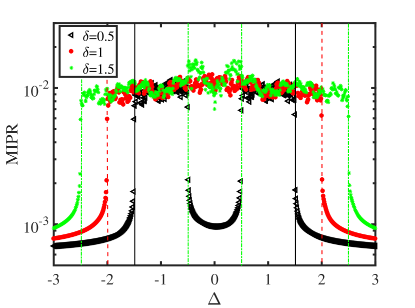
Figure 5: MIPR as a function of $p$-wave superfluid pairing $\Delta$ for the indicated values of modulation amplitude $\delta$. The dashed lines, dot-dashed lines, and solid lines demonstrate the abrupt changes of the MIPR at phase boundaries.

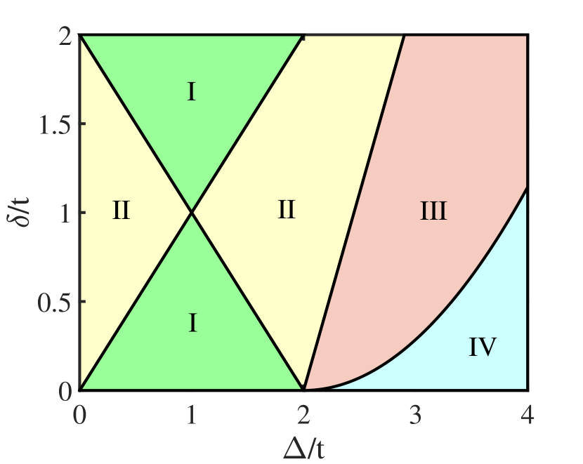
Figure 6: Phase diagram of the off-diagonal GAAH model with the $p$-wave incommensurate modulation amplitude $0<\delta\leq 2$ and the $p$-wave pairing strength $0\leq\Delta\leq 4$. The hopping incommensurate modulation amplitude is set to $\tau=1$ and the phase in the incommensurate modulation is set to $k_{y}=\pi/2$ and $\varphi=\beta\pi$. The phases are (I) localized phase, (II) critical localized phase, (III) critical extended phase, and (IV) extended phase.

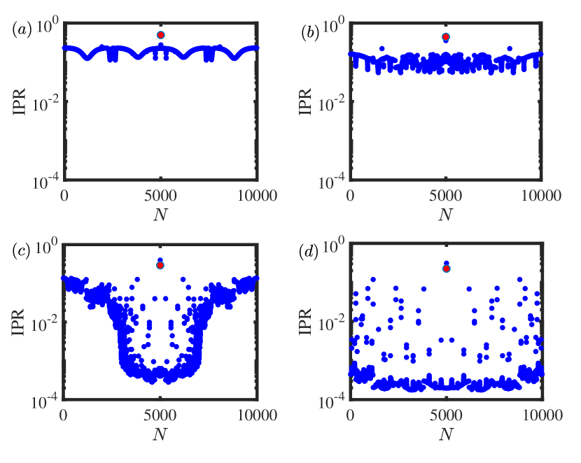
Figure 7: The distribution of IPRs over all the eigenstates for region (a) I (localized phase), (b) II (critical localized phase), (c) III (critical extended phase), and (d) IV (extended phase) of figure 6.

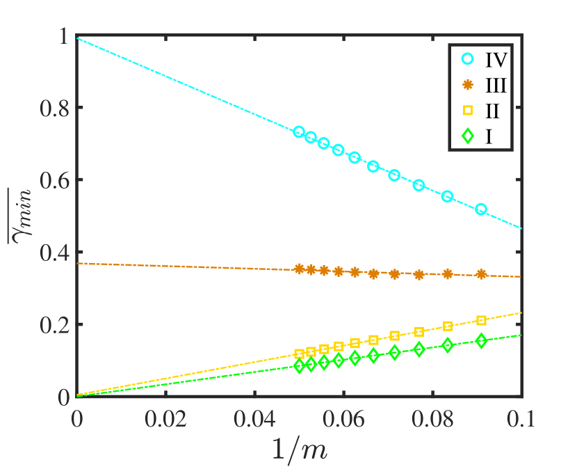
Figure 8: $\overline{\gamma_{min}}$ as function of $1/m$ for region I (localized phase), II (critical localized phase), III (critical extended phase), and IV (extended phase) of figure 6.

V.1 Off-diagonal GAAH model with $p$-wave pairing

The case $V=0$ corresponds to the off-diagonal GAAH model with $p$-wave pairing. We calculate the phase diagram as a function of the modulation strength of incommensurate $p$-wave pairing ($\delta$) and the modulation strength of incommensurate hopping ($\tau$), focusing mostly on the case $k_{y}=\pi/2$. We choose $\varphi=\beta\pi$. This off-diagonal GAAH model in the limit $\Delta=0$ and $\delta=0$ exhibits nontrivial zero-energy edge modes Ganeshan13 ; Cestari16 and in a large parameter space preserves the critical states Liu15 . We find that the topological properties and localization of this system are profoundly affected by a finite $\delta$. The main new feature compared to Ref. Liu15, is various phases with mobility edges. The phase diagram based on the MIPR of the off-diagonal GAAH model with $p$-wave pairing (without hopping modulations and site-diagonal potential), is shown in Fig. 2. The extended phase (regions I and II), the mobility-edge phase (region III) and critical phase (region IV) are separated by the black solid lines. Regions I, II, and III host two zero-energy modes as a result of nontrivial topology which only appear for open boundary conditions. In Fig. 3, we show the distribution of the inverse participation ratio (IPR) for different eigenstates. In region I (Fig. 3(a)), II (Fig. 3(b)) and III (Fig. 3(c)), respectively, we find the zero-energy topological edge modes (large red dots) indicating the topologically nontrivial phase. For almost all eigenstates, the IPR distribution has the same characteristics (around $10^{-4}$) in regions I and II, which shows that all the eigenstates are extended. In regions III and IV, the value of IPR is around $10^{-2}$ which is two orders of magnitude larger than in the extended phase. These dispersed distributions suggests that these regions (III and IV) are critical phases. These results confirm that regions I, II, and III are in the nontrivial-topological phases, while the region IV is trivial phase. Also, as shown in Fig. 4, region IV is topologically trivial and the edge modes (indicated in red color in the figure), in the regions I and III are found to be very robust. For comparison, in Ref. Cestari16 the robustness of edge states against modulated on-site potential was studied, and there a critical potential strength was found beyond which the edge states ceased to exist. Here, the edge states in occur in the case of off-diagonal disorder when $\tau=0$ and in principle survive after the model undergoes Anderson-like localization.

The evolution of the MIPR on a logarithmic scale at three values of $\delta=0.5$, $1$, and $1.5$ is shown in Fig. 5. We find that the MIPR changes abruptly from one phase to another as a function of $\Delta$ and $\delta$. There are four turning points and the change of MIPR at these points becomes sharper with increasing system size $L$ (results not shown). Thus, in the thermodynamic limit $L\rightarrow\infty$, a discontinuity at the turning points signals the phase transitions among the mobility-edge, the extended, and the critical phases.

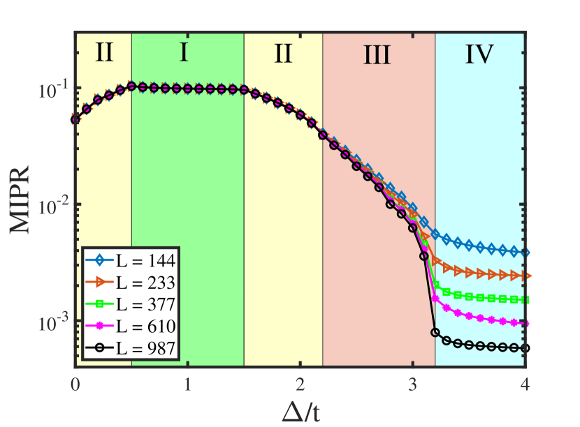
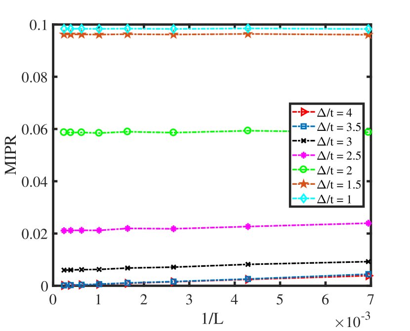
Figure 9: Upper panel: MIPR (log-scale) as a function of $p$-wave superfluid pairing $\Delta/t$ for different chain lengths $L$ for $\tau=1$ and $\delta=0.5$. Bottom panel: MIPR with the inverse system size $1/L$. For the extended phase, MIPR tends to zero as $L$ increases.

We have also considered the dependence of the phase diagram on nonzero $\tau$. By calculating the MIPR, we find that the localization properties of this model are significantly affected by turning on the off-diagonal hopping modulation of $\tau$. For $\tau=1$, the results are summarized in the phase diagram shown in Fig. 6. There are four distinct phases, localized phase (I), critical localized phase (II), critical extended phase (III), and extended phase (IV), separated by solid black lines. In Fig. 7, we show examples of the distribution of IPR over different eigenstates for localized phase (I), critical localized phase (II), critical extended phase (III), and extended phase (IV) of Fig. 6. Topological edge states are found in all phases. An interesting situation is depicted in Fig. 7 (c): the MIPR indicates the simultaneous presence of localized and extended states, as in a mobility edge phase, but here the boundary is smeared between the two. As the eigenenergy increases in Fig. 7(c), the IPR smoothly changes from a typical value for the localized stets around $10^{-1}$ to a typical value for the extended states $10^{-4}$. The smooth changes of the IPR suggest that there exist the semi-mobility edge in the energy spectrum. Also, for these selected phases in Fig. 8, we plotted $\overline{\gamma}_{min}$ as a function of $1/m$. For the localized phase, $\overline{\gamma}_{min}$ extrapolates to $0$ and but critical localized phase, $\overline{\gamma}_{min}$ vanish to zero. Furthermore, for critical extended phase $\overline{\gamma}_{min}$ extrapolates to $0.38$, but for extended phase $\overline{\gamma}_{min}$ extrapolates to $1$. These results also confirm our phase diagram in Fig. 6.

Fig. 9 shows the MIPR of the model as a function of $\Delta$ with $\tau=1$ and $\delta=0.5$ for different system sizes. We have checked that with increasing $L$, the system is in the localized region (I) for $\delta-\tau+1<\Delta<\tau-\delta+1$. Also, for the extended phase (III) the MIPR is finite and depend on the system size ($L$). In this phase, the MIPR satisfies the finite size scaling (FSS) form, $\textmd{MIPR}=bL^{-\eta}$. At the $\Delta/t=3.5$, $\eta=0.63$. For this phase, with the increase of $L$, MIPR tends to zero. The MIPR among localized, critically localized, critical extended, and extended phases satisfies

$$\textmd{MIPR}_{E}<\textmd{MIPR}_{CE}<\textmd{MIPR}_{CL}<\textmd{MIPR}_{L}$$ (26)

We verified this expression by checking the FSS in the whole phase diagram (results not shown).

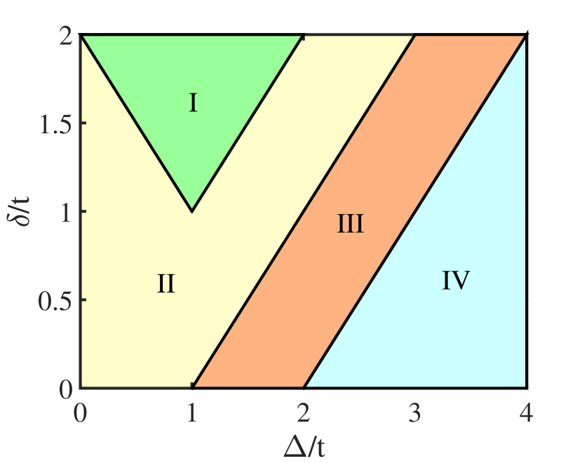
Figure 10: Phase diagram of the generic GAAH model with the $p$-wave incommensurate modulation amplitude $0<\delta\leq 2$ and the $p$-wave pairing strength $0\leq\Delta\leq 4$. The hopping incommensurate modulation amplitude is set to $\tau=1$, the on-site potential incommensurate modulation amplitude is set to $V/t=1$, and the phase in the incommensurate modulation is set to $k_{y}=\pi/2$ and $\varphi=\beta\pi$. The phases are (I) localized phase, (II) critical localized phase, (III) critical extended phases, (IV) extended phases.

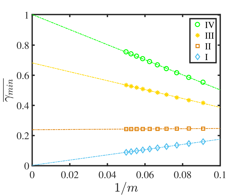
Figure 11: $\overline{\gamma_{min}}$ as function of $1/m$ for region I (localized phase), II (critical localized phase), III (critical extended phase), and IV (extended phase) of figure 10.

Figure 12: The distribution of IPRs over all the eigenstates for (a) region I (localized phase), (b) II (critical localized phase), (c) III (critical extended phase), and (d) IV (extended phase) of figure 10.

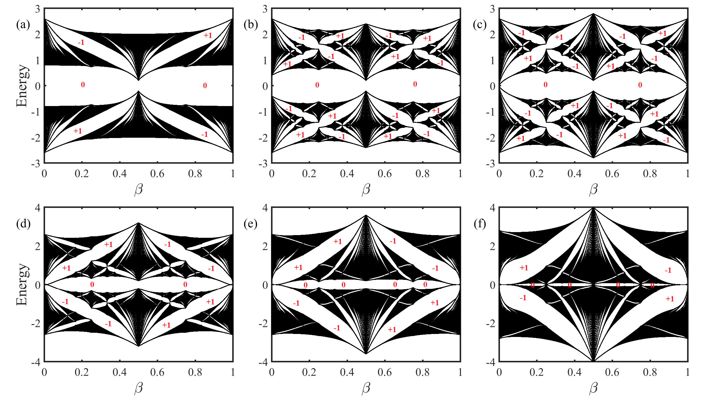
Figure 13: Hofstadter butterfly: energy spectrum as a function of magnetic flux per plaquette $\beta$ in Aubry-André lattice with $V=0$, $\tau=0.3$, $\Delta=0.4$, and (a) $\delta=0$, (b) $\delta=0.2$, (c) $\delta=0.4$, (d) $\delta=0.6$, (e) $\delta=0.8$, (f) $\delta=1$.

V.2 Generic GAAH model with $p$-wave pairing

We also investigate the generic $p$-wave pairing GAAH model with modulated on-site potentials, modulated off-diagonal hopping terms and modulated $p$-wave pairing terms. In this section, we explore the influence of the modulated on-site potential on the phase transition. It is clear that varying $V$ changes the phase diagram. So due to the modulation in the $p$-wave pairing term, we find that the system has a stronger tendency to become extended as a function of $\Delta/t$ when the disordered on-site potential ($V$) is varied. In Fig. 10, the phase diagram of the generic GAAH model for the case $V/t=1$ is shown. The phase boundary separating the localized phase, critical localized phase, critical extended phases, and extended phases vary rapidly with the SC pairing. We also performed a FSS analysis for this phase diagram (results not shown). When $V/t=1$, it is clear that for $\delta/t<1$, the localized phase disappears and the critical localized phase increases sharply. We also focus on the distribution of IPR with different eigenstates and multifractal analysis Hiramoto89 for this case. Example of determining $\overline{\gamma}_{min}$ as a function of $1/m$ in phases I, II, III, and IV of Fig. 10 is shown in Fig. 11. For this phase diagram, $\overline{\gamma}_{min}$ extrapolates to $0$ if we are in I-phase (in this case, the multifractal analysis of the wave function shows that all wave functions are in localized states) and to $1$ if are in IV-phase (in this case, the multifractal analysis of wave function shows that all of the wave functions are in extended state). The distribution of IPR in the eigenstates, shown in Fig. 12, indicates that almost all the eigenstates IPR are close to each other in phase I (being around $10^{-1}$) and phase IV (being around $10^{-4}$). For phases II and III, the multifractal analysis of wave function is shown in Fig. 11 (b) and Fig. 11 (c). For the critical localized phase (II), $\overline{\gamma}_{min}$ extrapolates to $0.245$ and for the critical extended phase (III,) $\overline{\gamma}_{min}$ extrapolates to $0.685$. Again, as in Fig. 8, all phases exhibit topological edge modes. As the eigenenergy increases in Fig. 12(b) for the critical localized state, the IPR suddenly jumps from a typical value for the localized states around $10^{-1}$ to a typical value for the extended states $10^{-4}$, but for the critical extended state this happens twice (see Fig. 12(c)). Models of which we are aware Sarma10 ; Liu15 show one mobility edge jump. Recall that in Fig. 8 it was also the critical extended state which showed unusual behavior, the smeared mobility edge.

In summary we find that due to the modulation in the SC pairing the incommensurate generic GAAH model with $p$-wave pairing delocalizes easier when varying the disordered on-site potential, when $\delta<V$. We find that the topological properties of the generic GAAH model with $p$-wave pairing are significantly affected by turning on the modulated on-site potential and modulated $p$-wave SC pairing.

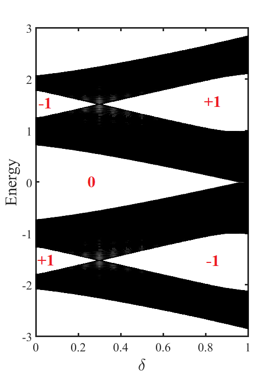
Figure 14: The evolution of the energy bands for $\beta=0.25$, $V=0$, $\tau=0.3$, and $\Delta=0.4$ as function of $\delta$ shown in Fig. (13). Gaps are labeled with their Chern numbers.

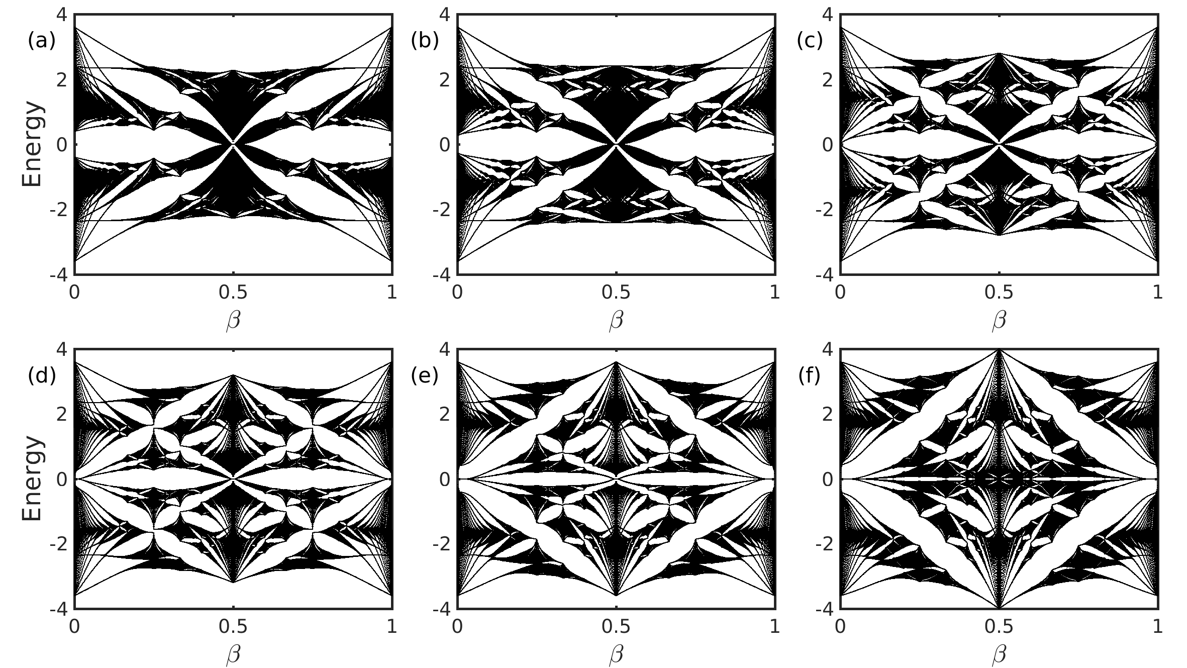
Figure 15: Hofstadter butterfly: energy spectrum as a function of magnetic flux per plaquette $\beta$ in Aubry-André lattice with $V=1$, $\tau=0.3$, $\Delta=0.4$, and (a) $\delta=0$, (b) $\delta=0.2$, (c) $\delta=0.4$, (d) $\delta=0.6$, (e) $\delta=0.8$, (f) $\delta=1$.

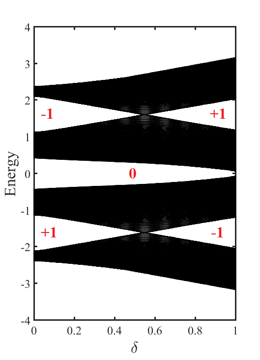
Figure 16: The evolution of the energy bands for $\beta=0.25$, $V=1$, $\tau=0.3$, and $\Delta=0.4$ as function of $\delta$ shown in Fig. (15). Gaps are labeled with their Chern numbers.

VI Commensurate modulation

When $\beta$ is rational, the lattice is commensurate. It is known that in the commensurate case Zeng16 , the system will not undergo a localization-delocalization transition as in the incommensurate case. When $\beta=1/2$, both Kitaev-like and Su-Schrieffer-Heeger-like (SSH-like) models are included in this GAAH model with $p$-wave SC pairing for commensurate modulations. The Hamiltonian of Eq. (1) is reduced to the SSH model for $V=\Delta=\delta=0$ and to the Kitaev model for $\tau=\delta=0$. In order to determine the different phase boundaries and characterize the topological phases, we need to calculate the effect of modulated SC pairing on the topological properties of the system. In the following, we characterize the topological nature of the modulated SC pairing by calculating the evolution of Chern numbers Avron83 for the major gaps of the spectrum.

VI.1 Chern numbers

Figure 17: The evolution of the energy bands for $\beta=0.25$, $V=1$, $\tau=0.3$, and $\Delta=0.4$ as function of $\delta$ shown in Fig. (15). Gaps are labeled with their Chern numbers.

Chern numbers can be calculated from the density with respect to changes in the magnetic field using the Středa formula Streda82 ; Umucallar08 . In lattice systems, the Chern number can be written as

$$C=\frac{\partial\bar{n}(\beta)}{\partial\beta}$$ (27)

where $\bar{n}$ is the number of levels below the Fermi level. This formula is valid when the chemical potential lies in a gap Streda82 . Formally, the evaluation of the Chern numbers can be calculated by $k$-space integration of the Berry curvature over the Brillouin zone. In Fig. 13 we present the Hofstadter butterfly for the case $V/t=0$, $\lambda=0.3$, $\Delta=0.4$ and various values of $\delta$. The spectrum for $\delta=0$ is clearly formed by two triangular-lattice Hofstadter butterflies separated by a large gap. The Hofstadter butterfly separation is controlled by the SC parameter, $\delta$ (see Fig. 13). As illustrated in this figure, by changing $\delta$, the upper (lower) butterfly approaches the square regime and then the honeycomb regime, which has different topology (in other words at the $\beta=0.2$ for upper lattice the Chern number changes from $-1$ to $1$). Also, we see that as $\delta$ is increased, the gaps at zero-energy are sufficiently small and have not completely closed so that the overall the butterfly shape is maintained. It is possible to understand this surprising result by considering the evolution of the energy bands at the points at which the main gap closes and reopens. For $V/t=0$, $\lambda=0.3$, $\Delta=0.4$, and $\beta=0.25$, these evolutions are demonstrated in Fig. 14. When the energy gap closes and reopens through this evolution, Chern numbers will change. For this case, we find two different regions corresponding to different Chern numbers, $\pm 1$. An important observation is that the Chern number is sensitively to the $\delta$ parameter. As can be seen in Fig. 14, the whole area is covered by the triangular lattice, while the square lattice is confined to the point at gap closure, $\delta=0.3$.

For the second case we consider $V\neq 0$, when the system has sublattice asymmetry. In this case, we can see that when $V\neq 0$, the evolution of the energy spectrum between the triangular lattice and the square lattice remain unchanged (see Fig. 15). More interestingly, in this case, parts of the energy modes in the topologically nontrivial regime split into two energy modes which can be taken as two 1D Majorana chains coupled by the on-site potential. As an example in Fig. 17, we display the evolution of bands from the triangular to the square and then triangular with different topology. As is shown in this figure, when $V$ becomes nonzero and gets stronger, the critical value of the phase transition $\delta_{c}$ is increased.

VII CONCLUSION

In this paper, we studied a GAAH model with modulated $p$-wave SC-pairing, both in the commensurate and incommensurate cases. We mapped derived the 2D magnetic analog of the model, have shown that in the bipartite commensurate case four different topological excitations are possible, mapped the phase diagram of the model via studying the localization characteristics, and studied the evolution of its Hofstadter butterflies. The phase diagram is remarkably rich, exhibiting localized, extended, and critical phases, as well as topological edge states, which can occur in extended or critical cases. Several new phases were revealed, unique to the model with modulated $p$-wave pairing: in the critical extended phase when incommensurate $p$-wave pairing and hopping is turned on, the change change in inverse participation ratios separating extended and localized regions is smeared, rather than sharp, as it happens Liu18 in the extended GAAH model without $p$-wave pairing modulation. When, in addition, the on-site potential is modulated the jumps between extended and localized regions are again sharp, but increase in number. For the commensurate case the modulated SC amplitude results in Hofstadter butterfly plots showing a transition from the rectangular to the square lattice as the parameter $\delta$ varies.

References

- (1) P.W. Anderson, Phys. Rev. 109 1492 (1958).
- (2) F. Evers, A.D. Mirlin, Rev. Mod. Phys. 80 1355 (2008).
- (3) E. Abrahams (Ed.), 50 Years of Anderson Localization, World Scientific, Singapore, 2010.
- (4) H. Shima, T. Nomura and T. Nakayama, Phys. Rev. B 70 075116 (2004).
- (5) F.M. Izrailev , A. A. Krokhin and N. M. Makarov, Phys. Rep. 512 125 (2012).
- (6) J. Biddle, D.J. Priour Jr., B. Wang, and S. Das Sarma, Phys. Rev. B 83 075105 (2011).
- (7) Y. Zhang, D. Bulmsh, A.V. Maharaj, C.-M. Jian, S.A. Kivelson, arXiv:1504.05205 (2015)
- (8) Y. Wang, G. Xianlong, and S. Chen, Eur. Phys. J. B 90 215 (2017).
- (9) S. Aubry and G. André, Ann. Israel Phys. Soc. 3 133 (1980).
- (10) P. G. Harper, Proc. Phys. Soc. A 68 874 (1955).
- (11) C. Aulbach, A. Wobst, G-L. Ingold, P. Hänggi and I. Varga, New J. Phys., 6 70 (2004).
- (12) Y. E. Kraus, Y. Lahini, Z. Ringel, M. Verbin, and O. Zilberberg, Phys. Rev. Lett. 109, 106402 (2012).
- (13) L.-J. Lang, X. Cai, and S. Chen, Phys. Rev. Lett. 108, 220401 (2012).
- (14) Y. E. Kraus and O. Zilberberg, Phys. Rev. Lett. 109, 116404 (2012).
- (15) Q. B. Zeng , S. Chen and R. Lü, Phys. Rev. B 94 125408 (2016).
- (16) W.P. Su, J. R. Schrieffer, and A. J. Heeger, Phys. Rev. Lett. 42 1698 (1979).
- (17) R. Wakatsuki, M. Ezawa, Y. Tanaka, and N. Nagaosa, Phys. Rev. B 90 014505 (2014).
- (18) A. Y. Kitaev, Phys.-Usp. 44 131 (2001).
- (19) D. J. Thouless, Phys. Rev. Lett. 61, 2141 (1988).
- (20) S. Das Sarma, S. He, and X. C. Xie, Phys. Rev. Lett. 61, 2144 (1988).
- (21) J. Biddle and S. Das Sarma, Phys. Rev. Lett. 104, 070601 (2010).
- (22) T. Liu, P. Wang, S. Chen, and G. Xianlong, J. Phys. B: At. Mol. Opt. Phys. 51 025301 (2018).
- (23) A. Altland, M. R. Zirnbauer, Phys. Rev. B 55 1142 (1997).
- (24) J.C.C. Cestari, A. Foerster and M. A. Gusmão, Phys. Rev. B 93, 205441 (2016).
- (25) F. Liu, S. Ghosh, and Y. D. Chong, Phys. Rev. B 91, 014108 (2015).
- (26) S. Ganeshan, K. Sun, and S. Das Sarma, Phys. Rev. Lett. 110, 180403 (2013).
- (27) G. Roati, C. D’Errico, L. Fallani, M. Fattori, C. Fort, M. Zaccanti, G. Modugno, M. Modugno, and M. Inguscio, Nature (London) 453, 895 (2008).
- (28) J. Chabé, G. Lemarié, B. Grémaud, D. Delande, P. Szriftgiser, and J. C. Garreau, Phys. Rev. Lett. 101, 255702 (2008).
- (29) L. Dal Negro, C. J. Oton, Z. Gaburro, L. Pavesi, P. Johnson, A. Lagendijk, R. Righini, M. Colocci, and D. S. Wiersma, Phys. Rev. Lett. 90, 055501 (2003).
- (30) Y. Lahini, R. Pugatch, F. Pozzi, M. Sorel, R. Morandotti, N. Davidson, and Y. Silberberg, Phys. Rev. Lett. 103, 013901 (2009).
- (31) D. R. Hofstadter, Phys. Rev. B 14, 2239 (1976).
- (32) Y. E. Kraus, Y. Lahini, Z. Ringel, M. Verbin, and O. Zilberberg, Phys. Rev. Lett. 109, 106402 (2012).
- (33) E. Lieb, T. Schultz, and D. Mattis, Ann. Phys. (N.Y.) 16, 407 (1961).
- (34) X. Cai, L.-J. Lang, S. Chen, and Y. Wang, Phys. Rev. Lett. 110, 176403 (2013).
- (35) H. Hiramoto and M. Kohmoto, Phys. Rev. B 40, 8225 (1989).
- (36) J. H. Han, D. J. Thouless, H. Hiramoto, and M. Kohmoto, Phys. Rev. B 50, 11365 (1994).
- (37) P. G. de Gennes, Superconductivity of Metals and Alloys (Benjamin, New York, 1966).
- (38) M. Kohmoto and D. Tobe, Phys. Rev. B 77, 134204 (2008).
- (39) J. Wang, X.-J. Liu, G. Xianlong, and H. Hu, Phys. Rev. B 93, 104504 (2016).
- (40) D. J. Thouless, J. Phys. C: Solid State Phys. 5, 77 (1972).
- (41) M. Kohmoto, Phys. Rev. Lett. 51, 1198(1983).
- (42) J. E. Avron, R. Seiler, and B. Simon, Phys. Rev. Lett. 51, 51 (1983).
- (43) P. Středa, J. Phys. C 15, L717 (1982).
- (44) R. O. Umucalilar, H. Zhai, and M. Ö. Oktel, Phys. Rev. Lett. 100, 070402 (2008).