Progressive Perception-Oriented Network
for Single Image Super-Resolution

Abstract

Recently, it has been demonstrated that deep neural networks can significantly improve the performance of single image super-resolution (SISR). Numerous studies have concentrated on raising the quantitative quality of super-resolved (SR) images. However, these methods that target PSNR maximization usually produce blurred images at large upscaling factor. The introduction of generative adversarial networks (GANs) can mitigate this issue and show impressive results with synthetic high-frequency textures. Nevertheless, these GAN-based approaches always have a tendency to add fake textures and even artifacts to make the SR image of visually higher-resolution. In this paper, we propose a novel perceptual image super-resolution method that progressively generates visually high-quality results by constructing a stage-wise network. Specifically, the first phase concentrates on minimizing pixel-wise error, and the second stage utilizes the features extracted by the previous stage to pursue results with better structural retention. The final stage employs fine structure features distilled by the second phase to produce more realistic results. In this way, we can maintain the pixel, and structural level information in the perceptual image as much as possible. It is useful to note that the proposed method can build three types of images in a feed-forward process. Also, we explore a new generator that adopts multi-scale hierarchical features fusion. Extensive experiments on benchmark datasets show that our approach is superior to the state-of-the-art methods. Code is available at https://github.com/Zheng222/PPON.

1 Introduction

Due to the emergence of deep learning for other fields of computer vision studies, the introduction of convolutional neural networks (CNNs) has dramatically advanced SR’s performance. For instance, the pioneering work of the super-resolution convolution neural network (SRCNN) proposed by Dong et al.  [1, 2] employed three convolutional layers to approximate the nonlinear mapping function from interpolated LR image to HR image and outperformed most conventional SR methods [3, 4]. Various works [5, 6, 7, 8, 9, 10, 11, 12, 13, 14, 15, 16] that explore network architecture designs and training strategies have continuously improved SR performance in terms of quantitative quality such as peak signal-to-noise ratio (PSNR), root mean squared error (RMSE), and structural similarity (SSIM) [17]. However, these PSNR-oriented approaches still suffer from blurry results at large upscaling factors, e.g., $4\times$, particularly concerning the restoration of delicate texture details in the original HR image, distorted in the LR image.

In recent years, several perceptual-related methods have been exploited to boost visual quality under large upscaling factors [18, 19, 20, 21, 22]. Specifically, the perceptual loss is proposed by Johnson et al.  [18], which is a loss function that measures differences of the intermediate features of VGG19 [23] when taking the ground-truth and generated images as inputs. Legig et al.  [19] extend this idea by adding an adversarial loss [24] and Sajjadi et al.  [20] combine perceptual, adversarial and texture synthesis losses to produce sharper images with realistic textures. Wang et al.  [25] incorporate semantic segmentation maps into a CNN-based SR network to generate realistic and visually pleasing textures. Although these methods can produce sharper images, they typically contain artifacts that are readily observed.

Moreover, these approaches tend to improve visual quality without considering the substantial degradation of quantitative quality. Since the primary objective of the super-resolution task is to make the enlarged images resemble the ground-truth HR images as much as possible, it is necessary to maintain nature while guaranteeing the basic structural features that is related to pixel-to-pixel losses e.g., mean squared error (MSE), mean absolute error (MAE). At present, the most common way is to pre-train a PSNR-oriented model and then fine-tune this pre-trained model, in company with a discriminator network and perceptual loss. Even though this strategy helps increase the stability of the training process, it still requires updating all parameters of the generator, which means an increase in training time.

In this paper, we propose a novel super-resolution method via the progressive perception-oriented network (PPON), which gradually generates images with pleasing visual quality. More specifically, inspired by [26], we propose a hierarchical feature fusion block (HFFB) as the basic block (shown in Figure 3(a)), which utilizes multiple dilated convolutions with different rates to exploit abundant multi-scale information. In order to ease the training of very deep networks, we assemble our basic blocks by using residual-in-residual fashion [16, 22] named residual-in-residual fusion block (RRFB) as illustrated in Figure 3(b). Our method adopts three reconstruction modules: a content reconstruction module (CRM), a structure reconstruction module (SRM), and a photo-realism reconstruction module (PRM). The CRM as showed in Figure 1 mainly restores global information and minimizes pixel-by-pixel errors as previous PSNR-oriented approaches. The purpose of SRM is to maintain favorable structural information based on CRM’s result using structural loss. Analogously, PRM estimates the residual between the real image and the output of SRM with adversarial and perceptual losses. The diagrammatic sketch of this procedure is given in Figure 2. Since the input of the perceptual features extraction module (PFEM) contains fruitful structure-related features and the generated perceptual image is built on the result of SRM, our PPON can synthesize a visually pleasing image that provides not only high-frequency components but also structural elements.

To achieve rapid training, we develop a step-by-step training mode, i.e., our basic model (illustrated in Figure 1) is trained first, then we freeze its parameters and train the sequential SFEM and SRM, and so on. The advantage is that when we train perception-related modules (PFEM and PRM), very few parameters need to be updated. It differs from previous algorithms that they require to optimize all parameters to produce photo-realistic results. Thus, it will reduce training time.

Overall, our contributions can be summarized as follows.

• We develop a progressive photo-realism reconstruction approach, which can synthesize images with high fidelity (PSNR) and compelling visual effects. Specifically, we develop three reconstruction modules for completing multiple tasks, i.e., the content, structure, and perception reconstructions of an image. More broadly, we can also generate three images with different types in a feed-forward process, which is instructive to satisfy various task’s requirements.

• We design an effective training strategy according to the characteristic of our proposed progressive perception-oriented network (PPON), which is to fix the parameters of the previous training phase and utilize the features produced by this trained model to update a few parameters at the current stage. In this way, the training of the perception-oriented model is robust and fast.

• We also propose the basic model RFN mostly constructed by cascading residual-in-residual fusion blocks (RRFBs), which achieves state-of-the-art performance in terms of PSNR.

The rest of this paper is organized as follows. Section 2 provides a brief review of related SISR methods. Section 3 describes the proposed approach and loss functions in detail. In Section 4, we explain the experiments conducted for this work, experimental comparisons with other state-of-the-art methods, and model analysis. In Section 5, we conclude the study.

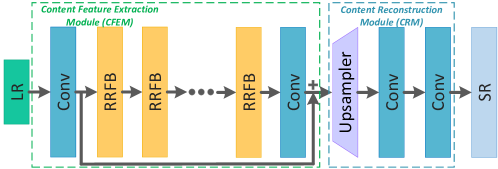
Figure 1: The network architecture of our basic PSNR-oriented model (Residual Fusion Network, namely RFN). We use 24 RRFBs for our experiments.

Figure 2: The architecture of our progressive perception-oriented network (PPON). CFEM indicates content feature extraction module in Figure 1. CRM, SRM, and PRM represent content reconstruction module, structural reconstruction module, and photo-realism reconstruction module, respectively. SFEM denotes structural features extraction module and PFEM describes the perceptual features extraction part. In addition, $\oplus$ is the element-wise summation operator.

(a) Hierarchical Feature Fusion Block (HFFB)

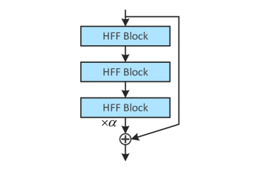
(b) Residual-in-Residual Fusion Block (RRFB)

Figure 3: The basic blocks are proposed in this work. (a) We employ 8 dilated convolutions. Each of them has 32 output channels for reducing block parameters. (b) RRFB is used in our primary and perception-oriented models and $\alpha$ is the residual scaling parameter [11, 22].

2 Related Work

In this section, we focus on deep neural network approaches to solve the SR problem.

2.1 Deep learning-based super-resolution

The pioneering work was done by Dong et al.  [1, 2], who proposed SRCNN for the SISR task, which outperformed conventional algorithms. To further improve the accuracy, Kim et al. proposed two deep networks, i.e., VDSR [6], and DRCN [7], which apply global residual learning and recursive layer respectively to the SR problem. Tai et al.  [9] developed a deep recursive residual network (DRRN) to reduce the model size of the very deep network by using a parameter sharing mechanism. Another work designed by the authors is a very deep end-to-end persistent memory network (MemNet) [12] for image restoration task, which tackles the long-term dependency problem in the previous CNN architectures. The methods mentioned above need to take the interpolated LR images as inputs. It inevitably increases the computational complexity and often results in visible reconstruction artifacts [10].

To speed up the execution time of deep learning-based SR approaches, Shi et al.  [8] proposed an efficient sub-pixel convolutional neural network (ESPCN), which extracts features in the LR space and magnifies the spatial resolution at the end of the network by conducting an efficient sub-pixel convolution layer. Afterward, Dong et al.  [5] developed a fast SRCNN (FSRCNN), which employs the transposed convolution to upscale and aggregate the LR space features. However, these two methods fail to learn complicated mapping due to the limitation of the model capacity. EDSR [11], the winner solution of NTIRE2017 [27], was presented by Lim et al. . This work is much superior in performance to previous models. To alleviate the difficulty of SR tasks with large scaling factors such as $8\times$, Lai et al.  [10] proposed the LapSRN, which progressively reconstructs the multiple SR images with different scales in one feed-forward network. Liu et al.  [28] used the phase congruency edge map to guide an end-to-end multi-scale deep encoder and decoder network for SISR. Tong et al.  [13] presented a network for SR by employing dense skip connections, which demonstrated that the combination of features at different levels is helpful for improving SR performance. Recently, Zhang et al.  [15] extended this idea and proposed a residual dense network (RDN), where the kernel is residual dense block (RDB) that extracts abundant local features via dense connected convolutional layers. Furthermore, the authors proposed very deep residual channel attention networks (RCAN) [16] that verified that the very deep network can availably improve SR performance and advantages of channel attention mechanisms. To leverage the execution speed and performance, IDN [14] and CARN [29] were proposed by Hui et al. and Ahn et al. , respectively. More concretely, Hui et al. constructed a deep but compact network, which mainly exploited and fused different types of features. And Ahn et al. designed a cascading network architecture. The main idea is to add multiple cascading connections from each intermediary layer to others. Such connections help this model performing SISR accurately and efficiently.

2.2 Super-resolution considering naturalness

SRGAN [19], as a landmark work in perceptual-driven SR, was proposed by Ledig et al. . This approach is the first attempt to apply GAN [24] framework to SR, where the generator is composed of residual blocks. To improve the naturalness of the images, perceptual and adversarial losses were utilized to train the model in SRGAN. Sajjadi et al.  [20] explored the local texture matching loss and further improved the visual quality of the composite images. Park et al.  [30] developed a GAN-based SISR method that produced realistic results by attaching an additional discriminator that works in the feature domain. Mechrez et al.  [21] defined the Contextual loss that measured the similarity between the generated image and a target image by comparing the statistical distribution of the feature space. Wang et al.  [22] enhanced SRGAN from three key aspects: network architecture, adversarial loss, and perceptual loss. A variant of Enhanced SRGAN (ESRGAN) won the first place in the PIRM2018-SR Challenge [31].

3 Proposed Method

3.1 The proposed PSNR-oriented SR model

The single image super-resolution aims to estimate the SR image $I^{\text{SR}}$ from its LR counterpart ${I^{\text{LR}}}$. An overall structure of the proposed basic model (RFN) is shown in Figure 1. This network mainly consists of two parts: content feature extraction module (CFEM) and reconstruction part, where the first part extracts content features for conventional image SR task (pursuing high PSNR value), and the second part naturally reconstructs ${I^{\text{SR}}}$ through the front features related to the image content. The first procedure could be expressed by

$${F_{c}}={H_{\text{CFE}}}\left({{I^{\text{LR}}}}\right),$$ (1)

where ${H_{\text{CFE}}\left(\cdot\right)}$ denotes content feature extractor, i.e., CFEM. Then, ${F_{c}}$ is sent to the content reconstruction module (CRM) ${H_{\text{CR}}}$,

$${I_{c}^{\text{SR}}}={H_{\text{CR}}}\left({{F_{c}}}\right)={H_{\text{RFN}}}\left({{I^{\text{LR}}}}\right),$$ (2)

where ${H_{\text{RFN}}\left(\cdot\right)}$ denotes the function of our RFN.

The basic model is optimized with the MAE loss function, followed by the previous works [11, 15, 16]. Given a training set $\left\{{I_{i}^{\text{LR}},I_{i}^{\text{HR}}}\right\}_{i=1}^{N}$, where $N$ is the number of training images, ${I_{i}^{\text{HR}}}$ is the ground-truth high-resolution image of the low-resolution image ${I_{i}^{\text{LR}}}$, the loss function of our basic SR model is

$${{\cal L}_{content}}\left(\Theta_{c}\right)=\frac{1}{N}\sum\limits_{i=1}^{N}{{{\left\|{{H_{\text{RFN}}}\left({I_{i}^{\text{LR}}}\right)-I_{i}^{\text{HR}}}\right\|}_{1}}},$$ (3)

where $\Theta_{c}$ denotes the parameter set of our content-oriented branch (COBranch), i.e., RFN.

3.2 Progressive perception-oriented SR model

As depicted in Figure 2, based on the content features extracted by the CFEM, we design a SFEM to distill structure-related information for restoring images with SRM. This process can be expressed by

$$I_{s}^{\text{SR}}={H_{\text{SR}}}\left({{F_{s}}}\right)+I_{c}^{\text{SR}}={H_{\text{SR}}}\left({{H_{\text{SFE}}}\left({{F_{c}}}\right)}\right)+I_{c}^{\text{SR}},$$ (4)

where ${H_{\text{SR}}}\left(\cdot\right)$ and ${{H_{\text{SFE}}}\left(\cdot\right)}$ denote the functions of SRM and SFEM, respectively. To this end, we employ the multi-scale structural similarity index (MS-SSIM) and multi-scale ${L_{1}}$ as loss functions to optimize this branch. SSIM is defined as

$$SSIM\left({x,y}\right)=\frac{{2{\mu_{x}}{\mu_{y}}+{C_{1}}}}{{\mu_{x}^{2}+\mu_{y}^{2}+{C_{1}}}}\cdot\frac{{2{\sigma_{xy}}+{C_{2}}}}{{\sigma_{x}^{2}+\sigma_{y}^{2}+{C_{2}}}}=l\left({x,y}\right)\cdot cs\left({x,y}\right),$$ (5)

where ${\mu_{x}}$, ${\mu_{y}}$ are the mean, ${{\sigma_{xy}}}$ is the covariance of $x$ and $y$, and ${C_{1}}$, ${C_{2}}$ are constants. Given multiple scales through a process of $M$ stages of downsampling, MS-SSIM is defined as

$$\text{MS-SSIM}(x,y)=l_{M}^{\alpha}\left({x,y}\right)\cdot\prod\limits_{j=1}^{M}{cs_{j}^{{\beta_{j}}}\left({x,y}\right)},$$ (6)

where ${l_{M}}$ and ${cs}_{j}$ are the term we defined in Equation 5 at scale $M$ and $j$, respectively. From [32], we set $\alpha={\beta_{M}}$ and $\beta=\left[{0.0448,0.2856,0.3001,0.2363,0.1333}\right]$. Therefore, the total loss function of our structure branch can be expressed by

$${{\cal L}_{\text{MS-SSIM}}}=\frac{1}{N}\sum\limits_{i=1}^{N}{\left[{1-\text{MS-SSIM}\left({I_{i}^{HR},{H_{\text{SOB}}}\left({F_{c}^{i}}\right)}\right)}\right]},$$ (7)

where ${H_{\text{SOB}}}\left(\cdot\right)$ represents the cascade of SFEM and SRM (light red area in Figure 5). $F_{c}^{i}$ denotes content features (see Equation 1) corresponding to $i$-th training sample in a batch. Thus, the total loss function of this branch can be formulated as follows

$${{\cal L}_{structure}\left(\Theta_{s}\right)}={{\cal L}_{\text{MS-L1}}}+\lambda{{\cal L}_{\text{MS-SSIM}}},$$ (8)

where ${{\cal L}_{\text{MS-L1}}}=\sum\limits_{j=1}^{M}{{\omega_{j}}\cdot{l_{mae}}\left({{x_{j}},{y_{j}}}\right)}$ and $\lambda$ is a scalar value to balance two losses, $\Theta_{s}$ denotes the parameter set of structure-oriented branch (SOBranch). Here, we set $M=5$, ${\omega_{1,2,...,5}}=[1,0.5,0.25,0.125,0.125]$ through experience.

Similarly, to obtain photorealistic images, we utilize structural-related features refined by SFEM and send them to our perception feature extraction module (PFEM). The merit of this practice is to avoid re-extracting features from the image domain. These extracted features contain abundant and superior quality structural information, which tremendously helps perceptual-oriented branch (POBranch, see in Figure 5) generate visually plausible SR images while maintaining the basic structure. Concretely, structural feature $F_{s}$ is entered in PFEM

$$I_{p}^{\text{SR}}={H_{\text{PR}}}\left({{F_{p}}}\right)+I_{s}^{\text{SR}}={H_{\text{PR}}}\left({{H_{\text{PFE}}}\left({{F_{s}}}\right)}\right)+I_{s}^{\text{SR}},$$ (9)

where ${H_{\text{PR}}}\left(\cdot\right)$ and ${{H_{\text{PFE}}}\left(\cdot\right)}$ indicate PRM and PFEM as shown in Figure 2, respectively. For pursuing better visual effect, we adopt Relativistic GAN [33] as in [22]. Given a real image ${x_{r}}$ and a fake one ${x_{f}}$, the relativistic discriminator intends to estimate the probability that ${x_{r}}$ is more realistic than ${x_{f}}$. In standard GAN, the discriminator can be defined, in term of the non-transformed layer ${C\left(x\right)}$, as $D\left(x\right)=\sigma\left({C\left(x\right)}\right)$, where $\sigma$ is sigmoid function. The Relativistic average Discriminator (RaD, denoted by $D_{\text{Ra}}$) [33] can be formulated as ${D_{\text{Ra}}}\left({{x_{r}},{x_{f}}}\right)=\sigma\left({C\left(x\right)-{\mathbb{E}_{{x_{f}}}}\left[{C\left({{x_{f}}}\right)}\right]}\right)$, if $x$ is real. Here, ${{\mathbb{E}_{{x_{f}}}}\left[{C\left(\cdot\right)}\right]}$ is the average of all fake data in a batch. The discriminator loss is defined by

$${\cal L}_{D}^{Ra}=-\mathbb{E}{{}_{{x_{r}}}}\left[{\log\left({{D_{Ra}}\left({{x_{r}},{x_{f}}}\right)}\right)}\right]-\mathbb{E}{{}_{{x_{f}}}}\left[{\log\left({1-{D_{Ra}}\left({{x_{f}},{x_{r}}}\right)}\right)}\right].$$ (10)

The corresponding adversarial loss for generator is

$${\cal L}_{G}^{Ra}=-\mathbb{E}{{}_{{x_{r}}}}\left[{\log\left({1-{D_{Ra}}\left({{x_{r}},{x_{f}}}\right)}\right)}\right]-\mathbb{E}{{}_{{x_{f}}}}\left[{\log\left({{D_{Ra}}\left({{x_{f}},{x_{r}}}\right)}\right)}\right].$$ (11)

where $x_{f}$ represents the generated images at the current perception-maximization stage, i.e., $I_{p}^{\text{SR}}$ in equation 9.

VGG loss that has been investigated in recent SR works [18, 19, 20, 22] for better visual quality is also introduced in this stage. We calculate the VGG loss based on the “conv5_4” layer of VGG19 [23],

$${{\cal L}_{vgg}}=\frac{1}{V}\sum\limits_{i=1}^{C}{{{\left\|{{\phi_{i}}\left({{I^{HR}}}\right)-{\phi_{i}}\left({I_{p}^{SR}}\right)}\right\|}_{1}}},$$ (12)

where $V$ and $C$ indicate the tensor volume and channel number of the feature maps, respectively, and ${{\phi_{i}}}$ denotes the $i$-th channel of the feature maps extracted from the hidden layer of VGG19 model. Therefore, the total loss for the perception stage is:

$${{\cal L}_{perception}\left(\Theta_{p}\right)}={{\cal L}_{vgg}}+\eta{\cal L}_{G}^{Ra},$$ (13)

where $\eta$ is the coefficients to balance these loss functions. And $\Theta_{p}$ is the training parameters of POBranch.

3.3 Residual-in-residual fusion block

We now give more details about our proposed RRFB structure (see Figure 3(b)), which consists of multiple hierarchical feature fusion blocks (HFFB) (see Figure 3(b)). Unlike the frequently-used residual block in SR, we intensify its representational ability by introducing the spatial pyramid of dilated convolutions [26]. Specifically, we develop $K$ $n\times n$ dilated convolutional kernels simultaneously, each with a dilation rate of $k$, $k=\left\{{1,\ldots,K}\right\}$. Due to these dilated convolutions preserve different receptive fields, we can aggregate them to obtain multi-scale features. As shown in Figure 4, single dilated convolution with a dilation rate of 3 (yellow block) looks sparse. The feature maps obtained using kernels of different dilation rates are hierarchically added to acquire an effective receptive field before concatenating them. A simple example is illustrated in Figure 4. For explaining this hierarchical feature fusion process clearly, the output of dilated convolution with a dilation rate of $k$ is denoted by $f_{k}$. In this way, concatenated multi-scale features $H_{ms}$ can be expressed by

$${H_{ms}}=\left[{{f_{1}},{f_{1}}+{f_{2}},\ldots,{f_{1}}+{f_{2}}+\cdots+{f_{K}}}\right].$$ (14)

After collecting these multi-scale features, we fuse them through a $1\times 1$ convolution $Con{v_{1\times 1}}$, that is $Con{v_{1\times 1}}\left({L{\mathop{\rm Re}\nolimits}LU\left({{F_{ms}}}\right)}\right)$. Finally, the local skip connection with residual scaling is utilized to complete our HFFB.

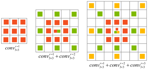
Figure 4: The diagrammatic sketch of multiple dilated convolutions addition. Taking the middle sub-figure as an example, $conv_{3\times 3}^{r=2}$ indicates $3\times 3$ dilated convolution with dilation rate of 2. Under the same conditions of receptive field, $conv_{3\times 3}^{r=1}+conv_{3\times 3}^{r=2}$ is more dense than $conv_{3\times 3}^{r=2}$.

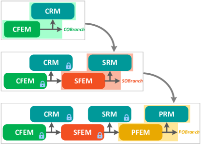
Figure 5: The training scheme for our PPON. The light green region (COBranch) in the first row is our basic model RFN. Light red and yellow areas represent SOBranch and POBranch mentioned in Section 3.2, respectively. The entire training process is split into 3 stages. The module with miniature lock means to freeze its parameters.

4 Experiments

4.1 Datasets and Training Details

We use the DIV2K dataset [27], which consists of 1,000 high-quality RGB images (800 training images, 100 validation images, and 100 test images) with 2K resolution. For increasing the diversity of training images, we also use the Flickr2K dataset [11] consisting of 2,650 2K resolution images. In this way, we have 3,450 high-resolution images for training purposes. LR training images are obtained by downscaling HR with a scaling factor of $4\times$ images using bicubic interpolation function in MATLAB. HR image patches with a size of $192\times 192$ are randomly cropped from HR images as the input of our proposed model, and the mini-batch size is set to 25. Data augmentation is performed on the 3,450 training images, which are randomly horizontal flip and 90-degree rotation. For evaluation, we use six widely used benchmark datasets: Set5 [34], Set14 [35], BSD100 [36], Urban100 [37], Manga109 [38], and the PIRM dataset [31]. The SR results are evaluated with PSNR, SSIM [17], learned perceptual image patch similarity (LPIPS) [39], and perceptual index (PI) on Y (luminance) channel, in which PI is based on the non-reference image quality measures of Ma et al.  [40] and NIQE [41], i.e., $\text{PI}=\frac{1}{2}\left({\left({10-\text{Ma}}\right)+\text{NIQE}}\right)$. The lower values of LPIPS and PI, the better.

As depicted in Figure 5, the training process is composed of three phases. First, we train the COBranch with Equation 3. The initial learning rate is set to $2\times{10^{-4}}$, which is decreased by 2 for every 1000 epochs ($1.38\times{10^{5}}$ iterations). And then, we fix the parameters of COBranch and only train the SOBranch through the loss function in Equation 8 with $\lambda=1\times{10^{3}}$. This process is illustrated in the second row of Figure 5. During this stage, the learning rate is set to $1\times{10^{-4}}$ and halved at every 250 epochs ($3.45\times{10^{4}}$ iterations). Similarly, we eventually only train the POBranch by Equation 13 with $\eta=5\times{10^{-3}}$. The learning rate scheme is the same as the second phase. All the stages are trained by ADAM optimizer [42] with the momentum parameter ${\beta_{1}}=0.9$. We apply the PyTorch v1.1 framework to implement our model and train them using NVIDIA TITAN Xp GPUs.

We set the dilated convolutions number as $K=8$ in the HFFB structure. All dilated convolutions have $3\times 3$ kernels and 32 filters, as shown in Figure 3(a). In each RRFB, we set the HFFB number as 3. In COBranch, we apply 24 RRFBs. Moreover, only 2 RRFBs are employed in both SOBranch and POBranch. All standard convolutional layers have 64 filters, and their kernel sizes are set to $3\times 3$ expect for that at the end of HFFB, whose kernel size is $1\times 1$. The residual scaling parameter $\alpha=0.2$ and the negative slope of LReLU is set as $0.2$.

4.2 Model analysis

Figure 6: PSNR performance and number of parameters. The results are evaluated on Set5 dataset for a scaling factor of $4\times$.

Model Parameters. We compare the trade-off between performance and model size in Figure 6. Among the nine models, RFN and RCAN show higher PSNR values than others. In particular, RFN scores the best performance in Set5. It should be pointed out that RFN uses fewer parameters than RCAN to achieve this performance. It does mean that RFN can better balance performance and model size.

Study of dilation convolution and hierarchical feature fusion. We remove the hierarchical feature fusion structure. Furthermore, in order to investigate the function of dilated convolution, we use ordinary convolutions. For validating quickly, only $1$ RRFB is used in CFEM, and this network is called RFN_mini. We conduct the training process with the DIV2K dataset, and the results are depicted in Table 1. As the number of RRFB increases, the benefits will increase accumulatively (see in Table 2).

Table 1: Investigations of dilated convolution and hierarchical fusion. These models are trained 200k iterations with DIV2K training dataset.

Dilated convolution	✗	✗	✓	✓
Hierarchical fusion	✗	✓	✗	✓
PSNR on Set5 $\left(4\times\right)$	31.68	31.69	31.63	31.72

Table 2: Investigations of dilated convolution. Above models are trained 300k iterations with DIV2K training dataset.

Method	N_blocks	Set5	Set14	BSD100	Urban100
w/o dilation	2	32.05	28.51	27.52	25.91
RFN_Mini	2	32.07	28.53	27.53	25.91
w/o dilation	4	32.18	28.63	27.59	26.16
RFN_Mini	4	32.26	28.67	27.60	26.23

PIRM_Val: 71 HR (a) (b) PPON

Figure 7: Ablation study of progressive structure. (a) w/o CRM & SOBranch. (b) w/o SOBranch.

Figure 8: The feature maps of CFEM, SFEM, and PFEM are visualized from left to right. Best viewed with zoom-in.

Table 3: Ablation study of progressive structure (with GAN). PSNR, SSIM, and PI are evaluated on the Y channel while LPIPS are conducted on the RGB color space.

Item	w/o CRM & SOBranch	w/o SOBranch	PPON
Memory footprint (M)	11,599	5,373	5,357
Training time (sec/epoch)	347	176	183
PIRM_Val (PSNR / SSIM / LPIPS / PI)	25.61 / 0.6802 / 0.1287 / 2.2857	26.32 / 0.6981 / 0.1250 / 2.2282	26.20 / 0.6995 / 0.1194 / 2.2353
PIRM_Test (PSNR / SSIM/ LPIPS / PI)	25.47 / 0.6667 / 0.1367 / 2.2055	26.16 / 0.6831 / 0.1309 / 2.1704	26.01 / 0.6831 / 0.1273 / 2.1511

Table 4: Performance of RFN and S-RFN (without GAN). All metrics are performed on the RGB color space.

Item	RFN	S-RFN
Memory footprint (M)	8,799	2,733
Training time (sec/epoch)	278	110
PIRM_Val (PSNR / SSIM / LPIPS)	27.27 / 0.8961 / 0.2901	27.14 / 0.7741 / 0.2651
PIRM_Test (PSNR / SSIM / LPIPS)	27.14 / 0.7571 / 0.3077	27.00 / 0.7637 / 0.2804
Set5 (PSNR / SSIM / LPIPS)	30.68 / 0.8714 / 0.1709	30.62 / 0.8737 / 0.1684
Set14 (PSNR / SSIM / LPIPS)	26.88 / 0.7543 / 0.2748	26.76 / 0.7595 / 0.2583
B100 (PSNR / SSIM / LPIPS)	26.52 / 0.7225 / 0.3620	26.40 / 0.7302 / 0.3377
Urban100 (PSNR / SSIM / LPIPS)	25.46 / 0.7940 / 0.1982	25.39 / 0.7982 / 0.1879
Manga109 (PSNR / SSIM / LPIPS)	29.71 / 0.8945 / 0.0984	29.62 / 0.8961 / 0.0939

4.3 Progressive structure analysis

HR	SRGAN [19]	ENet [20]	CX [21]	SuperSR [22]	ESRGAN [22]	PPON(Ours)

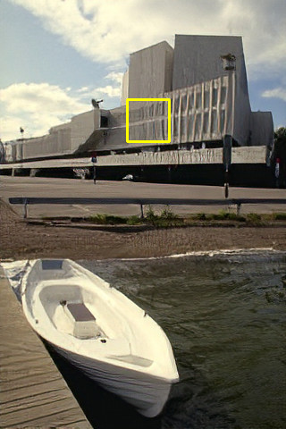
Figure 9: An example of the structure distortion. The image is from the BSD100 dataset [36].

SRc	SRs	SRp

Figure 10: A comparison of the visual effects between the three branch outputs. SRc, SRs, and SRp are outputs of the COBranch, SOBranch, and POBranch, respectively. The image is from the PIRM_Val dataset [31].

We observe that perceptual-driven SR results produced by GAN-based approaches [19, 20, 21] often suffer from structural distortion, as illustrated in Figure 9. To alleviate this problem, we explicitly add structural information through our devised progressive architecture described in the main manuscript. To make it easier to understand this progressive practice, we show an example in Figure 10. From this picture, we can note that the difference between SRc and SRp is mainly reflected in the sharper texture of SRp. Therefore, the remaining component is substantially the same. Please take into account this viewpoint, we naturally design the progressive topology structure, i.e., gradually adding high-frequency details.

To validate the feature maps extracted by the CFEM, SFEM, and PFEM have dependencies and relationships, we visualize the intermediate feature maps, as shown in Figure 8. From this picture, we can find that the feature maps distilled by three different extraction modules are similar. Thus, features extracted in the previous stage can be utilized in the current phase. In addition, feature maps in the third sub-figure contain more texture information, which is instructive to the reconstruction of visually high-quality images. To verify the necessity of using progressive structure, we remove CRM and SOBranch from PPON (i.e., changing to normal structure, similar to ESRGAN [22]). We observe that PPON without CRM & SOBranch cannot generate clear structural information, while PPON can better recover it. Table 3 suggests that our progressive structure can significantly improve the fidelity measured by PSNR and SSIM while improving perceptual quality. It indicates that fewer updatable parameters not only occupy less memory but also encourage faster training. “w/o CRM & SOBranch” is a fundamental architecture without proposed progressive structure, which consumes 11,599M memories. Once we turn to “w/o SOBranch”, the consumption of memory is reduced by 53.67%, and the training speed increased by 97.16%. Thus, our progressive structure is useful when training model with GAN. Comparing “w/o SOBranch” with PPON (LPIPS values), it naturally demonstrated that SOBranch is beneficial to improve perceptual performance. From Table 4, it can suggest that S-RFN occupies fewer memory footprints and obtains faster training speed than RFN. Besides, the perceptual performance (measured by LPIPS) of S-RFN is significantly improving than RFN evaluated on seven test datasets. Combining Table 3 with Table 4, we observe model with GAN (“w/o CRM & SOBranch”) requires more memories and longer training time. However, the perceptual performance of the model with GAN dramatically boosts than RFN. It means GAN is necessary for our architecture.

Few learnable model parameters (1.3M) complete task migration (i.e.from structure-aware to perceptual-aware) well in our work, while ESRGAN [22] uses 16.7M to generate perceptual results. We explicitly decompose a task into three subtasks (content, structure, perception). This approach is similar to human painting, first sketching the lines, then adding details. Our topology structure can quickly achieve the migration of similar tasks and infer multiple tasks according to the specific needs.

Figure 11: The inference architecture of our progressive perception-oriented network (PPON).

4.4 Difference to the previous GAN-based methods

Unlike the previous perceptual SR methods ( e.g., SRGAN [19], EnhanceNet [20], CX [21], and ESRGAN [22]), we employ the progressive strategy to gradually recover the fine-grained high-frequency details without sacrificing the structural information. As shown in Figure 11, we can obtain images with different perceptions by setting different values to $\alpha$. Now, Equation 9 can be modified as follows:

$$I_{p}^{\text{SR}}=\alpha\cdot{H_{\text{PR}}}\left({{F_{p}}}\right)+I_{s}^{\text{SR}}=\alpha\cdot{H_{\text{PR}}}\left({{H_{\text{PFE}}}\left({{F_{s}}}\right)}\right)+I_{s}^{\text{SR}}.$$ (15)

We provide an example (see in Figure 12) to demonstrate the effectiveness of this user-controlled adjustment of SR results.

$\alpha=0.0$	$\alpha=0.6$	$\alpha=1.0$

Figure 12: The perception-distortion trade-off. In the first column, $\alpha=0.0$ directly denotes the outputs of SOBranch. Equally, $\alpha=1.0$ indicates the results (without any discount) of POBranch. Best viewed with zoom-in.

4.5 Comparisons with state-of-the-art methods

Table 5: Quantitative evaluation results in terms of PSNR and SSIM. Red and blue colors indicates the best and second best methods, respectively. Here, S-RFN is the combination of RFN and SOBranch.

Method	Set5		Set14		B100		Urban100		Manga109
	PSNR	SSIM	PSNR	SSIM	PSNR	SSIM	PSNR	SSIM	PSNR	SSIM
Bicubic	28.42	0.8104	26.00	0.7027	25.96	0.6675	23.14	0.6577	24.89	0.7866
SRCNN [1]	30.48	0.8628	27.50	0.7513	26.90	0.7101	24.52	0.7221	27.58	0.8555
FSRCNN [5]	30.72	0.8660	27.61	0.7550	26.98	0.7150	24.62	0.7280	27.90	0.8610
VDSR [6]	31.35	0.8838	28.01	0.7674	27.29	0.7251	25.18	0.7524	28.87	0.8865
DRCN [7]	31.53	0.8854	28.02	0.7670	27.23	0.7233	25.14	0.7510	28.93	0.8854
LapSRN [10]	31.54	0.8852	28.09	0.7700	27.32	0.7275	25.21	0.7562	29.02	0.8900
MemNet [12]	31.74	0.8893	28.26	0.7723	27.40	0.7281	25.50	0.7630	29.42	0.8942
IDN [14]	31.82	0.8903	28.25	0.7730	27.41	0.7297	25.41	0.7632	29.41	0.8936
EDSR [11]	32.46	0.8968	28.80	0.7876	27.71	0.7420	26.64	0.8033	31.02	0.9148
SRMDNF [43]	31.96	0.8925	28.35	0.7772	27.49	0.7337	25.68	0.7731	30.09	0.9024
D-DBPN [44]	32.47	0.8980	28.82	0.7860	27.72	0.7400	26.38	0.7946	30.91	0.9137
RDN [15]	32.47	0.8990	28.81	0.7871	27.72	0.7419	26.61	0.8028	31.00	0.9151
MSRN [45]	32.07	0.8903	28.60	0.7751	27.52	0.7273	26.04	0.7896	30.17	0.9034
CARN [29]	32.13	0.8937	28.60	0.7806	27.58	0.7349	26.07	0.7837	30.47	0.9084
RCAN [16]	32.63	0.9002	28.87	0.7889	27.77	0.7436	26.82	0.8087	31.22	0.9173
SRFBN [46]	32.47	0.8983	28.81	0.7868	27.72	0.7409	26.60	0.8015	31.15	0.9160
SAN [47]	32.64	0.9003	28.92	0.7888	27.78	0.7436	26.79	0.8068	31.18	0.9169
RFN(Ours)	32.71	0.9007	28.95	0.7901	27.83	0.7449	27.01	0.8135	31.59	0.9199
S-RFN(Ours)	32.66	0.9022	28.86	0.7946	27.74	0.7515	26.95	0.8169	31.51	0.9211

Table 6: Results on public benchmark datasets, PIRM_Val, and PIRM_Test for existing perceptual quality specific methods and our proposed PPON ($\alpha=1.0$). Red color indicates the best performance and blue color indicates the second best performance.

Dataset	Scores	SRGAN [19]	ENet [20]	CX [21]	$\text{EPSR}_{2}$ [48]	$\text{EPSR}_{3}$ [48]	NatSR [49]	ESRGAN [22]	PPON (Ours)
Set5	PSNR	29.43	28.57	29.12	31.24	29.59	31.00	30.47	30.84
	SSIM	0.8356	0.8103	0.8323	0.8650	0.8415	0.8617	0.8518	0.8561
	PI	3.3554	2.9261	3.2947	4.1123	3.2571	4.1875	3.7550	3.4590
	LPIPS	0.0837	0.1014	0.0806	0.0978	0.0889	0.0943	0.0748	0.0664
Set14	PSNR	26.12	25.77	26.06	27.77	26.36	27.53	26.28	26.97
	SSIM	0.6958	0.6782	0.7001	0.7440	0.7097	0.7356	0.6984	0.7194
	PI	2.8816	3.0176	2.7590	3.0246	2.6981	3.1138	2.9259	2.7741
	LPIPS	0.1488	0.1620	0.1452	0.1861	0.1576	0.1765	0.1329	0.1176
B100	PSNR	25.18	24.94	24.59	26.28	25.19	26.45	25.32	25.74
	SSIM	0.6409	0.6266	0.6440	0.6905	0.6468	0.6835	0.6514	0.6684
	PI	2.3513	2.9078	2.2501	2.7458	2.1990	2.7746	2.4789	2.3775
	LPIPS	0.1843	0.2013	0.1881	0.2474	0.2474	0.2115	0.1614	0.1597
PIRM_Val	PSNR	N/A	25.07	25.41	27.35	25.46	27.03	25.18	26.20
	SSIM	N/A	0.6459	0.6747	0.7277	0.6657	0.7199	0.6596	0.6995
	PI	N/A	2.6876	2.1310	2.3880	2.0688	2.4758	2.5550	2.2353
	LPIPS	N/A	0.1667	0.1447	0.1750	0.1869	0.1648	0.1443	0.1194
PIRM_Test	PSNR	N/A	24.95	25.31	27.04	25.35	26.95	25.04	26.01
	SSIM	N/A	0.6306	0.6636	0.7068	0.6535	0.7090	0.6454	0.6831
	PI	N/A	2.7232	2.1133	2.2752	2.0131	2.3772	2.4356	2.1511
	LPIPS	N/A	0.1776	0.1519	0.1739	0.1902	0.1712	0.1523	0.1273

We compare our RFN with $16$ state-of-the-art methods: SRCNN [1, 2], FSRCNN [5], VDSR [6], DRCN [7], LapSRN [10], MemNet [12], IDN [14], EDSR [11], SRMDNF [43], D-DBPN [44], RDN [15], MSRN [45], CARN [29], RCAN [16], SAN [47], and SRFBN [46]. Table 5 shows quantitative comparisons for $\times 4$ SR. It can be seen that our RFN performs the best in terms of PSNR on all the datasets. The proposed S-RFN shows significant advantages of SSIM. In Figure 13, we present visual comparisons on different datasets. For image “img_011”, we observe that most of the compared methods cannot recover the lines and suffer from blurred artifacts. In contrast, our RFN can slightly alleviate this phenomenon and restore more details.

Urban100 ($4\times$): img_024 HR VDSR [6] LapSRN [10] DRRN [9] MemNet [12] PSNR/SSIM 19.38/0.5925 19.34/0.6037 19.51/0.6161 19.62/0.6179 EDSR [11] RDN [15] CARN [29] RCAN [16] RFN(Ours) 20.52/0.6826 20.62/0.6827 20.08/0.6449 21.13/0.7119 21.54/0.7304

Urban100 ($4\times$): img_011 HR VDSR [6] LapSRN [10] DRRN [9] MemNet [12] PSNR/SSIM 17.29/0.7565 17.21/0.7568 17.12/0.7660 17.29/0.7773 EDSR [11] RDN [15] CARN [29] RCAN [16] RFN(Ours) 18.42/0.8225 17.85/0.8003 17.71/0.7986 18.42/0.8224 19.17/0.8485

Urban100 ($4\times$): img_072 HR VDSR [6] LapSRN [10] DRRN [9] MemNet [12] PSNR/SSIM 19.19/0.7713 19.33/0.7836 19.91/0.8056 20.01/0.8099 EDSR [11] RDN [15] CARN [29] RCAN [16] RFN(Ours) 21.24/0.8573 21.12/0.8540 20.44/0.8297 21.46/0.8656 21.91/0.8745

Urban100 ($4\times$): img_028 HR VDSR [6] LapSRN [10] DRRN [9] MemNet [12] PSNR/SSIM 31.01/0.8683 30.97/0.8707 31.10/0.8702 31.10/0.8690 EDSR [11] RDN [15] CARN [29] RCAN [16] RFN(Ours) 31.95/0.8861 31.85/0.8833 31.42/0.8769 31.96/0.8857 32.37/0.8915

Manga109 ($4\times$): DualJustice HR VDSR [6] LapSRN [10] DRRN [9] MemNet [12] PSNR/SSIM 28.04/0.9201 28.30/0.9239 29.15/0.9356 29.28/0.9378 EDSR [11] RDN [15] CARN [29] RCAN [16] RFN(Ours) 31.55/0.9626 31.41/0.9617 30.46/0.9516 32.39/0.9688 33.01/0.9724

Figure 13: Visual comparisons for $4\times$ SR with RFN on Urban100 and Manga109 datasets.

BSD100 ($4\times$): 108005 HR SRGAN [19] ENet [20] CX [21] $\text{EPSR}_{2}$ [48] ESRGAN [22] S-RFN(Ours) PPON(Ours) PSNR/LPIPS 23.70/0.2471 23.27/0.2547 23.82/0.1999 25.72/0.2224 23.54/0.1806 26.48/0.2998 24.39/0.1546

BSD100 ($4\times$): 8023 HR SRGAN [19] ENet [20] CX [21] $\text{EPSR}_{2}$ [48] ESRGAN [22] S-RFN(Ours) PPON(Ours) PSNR/LPIPS 28.78/0.1355 25.71/0.3490 27.69/0.1610 29.97/0.2064 29.58/0.1554 31.17/0.2807 29.78/0.1332

PIRM_Val ($4\times$): 86 HR ENet [20] CX [21] $\text{EPSR}_{2}$ [48] ESRGAN [22] SuperSR [22] S-RFN(Ours) PPON(Ours) PSNR/LPIPS 24.16/0.1276 24.88/0.1248 26.79/0.1031 24.02/0.1189 25.03/0.1353 28.47/0.1352 26.32/0.0773

PIRM_Test ($4\times$): 223 HR ENet [20] CX [21] $\text{EPSR}_{3}$ [48] ESRGAN [22] SuperSR [22] S-RFN(Ours) PPON(Ours) PSNR/LPIPS 19.80/0.1756 20.64/0.1552 20.15/0.1797 18.96/0.2128 20.43/0.1710 23.11/0.2915 20.22/0.1466

PIRM_Val ($4\times$): 43 HR ENet [20] CX [21] EPSR3 [48] SuperSR [22] ESRGAN [22] PPON_128 (Ours) PPON (Ours) PSNR/LPIPS 24.77/0.1560 25.55/0.1466 24.53/0.2305 25.12/0.1421 23.80/0.1861 24.57/0.1320 24.87/0.1256

PIRM_Val ($4\times$): 64 HR ENet [20] CX [21] EPSR3 [48] SuperSR [22] ESRGAN [22] PPON_128 (Ours) PPON (Ours) PSNR/LPIPS 25.04/0.1429 25.60/0.1301 25.36/0.1597 25.60/0.1468 24.56/0.1513 25.84/0.1092 25.91/0.1067

PIRM_Val ($4\times$): 84 HR ENet [20] CX [21] EPSR3 [48] SuperSR [22] ESRGAN [22] PPON_128 (Ours) PPON (Ours) PSNR/LPIPS 24.12/0.1795 25.03/0.1697 22.55/0.3107 24.07/0.1632 22.73/0.2307 24.37/0.1461 23.99/0.1547

PIRM_Test ($4\times$): 248 HR ENet [20] CX [21] EPSR3 [48] SuperSR [22] ESRGAN [22] PPON_128 (Ours) PPON (Ours) PSNR/LPIPS 23.82/0.2265 24.83/0.1891 23.80/0.2250 23.06/0.2323 22.55/0.2782 24.62/0.1593 24.26/0.1544

PIRM_Test ($4\times$): 258 HR ENet [20] CX [21] EPSR3 [48] SuperSR [22] ESRGAN [22] PPON_128 (Ours) PPON (Ours) PSNR/LPIPS 19.92/0.2776 20.41/0.2504 20.27/0.2938 20.54/0.2616 18.67/0.2741 20.17/0.2202 20.43/0.2068

Figure 14: Qualitative comparisons of perceptual-driven SR methods with our results at scaling factor of 4. Here, SuperSR is the variant of ESRGAN and it won the first place in the PIRM2018-SR Challenge.

Table 6 shows our quantitative evaluation results compared with $6$ perceptual-driven state-of-the-arts approaches: SRGAN [19], ENet [20], CX [21], EPSR [48], NatSR [49], and ESRGAN [22]. The proposed PPON achieves the best in terms of LPIPS and keep the presentable PSNR values. For image “86” in Figures 14, the result generated by S-RFN is blurred but has a elegant structure. Based on S-RFN, our PPON can synthesize realistic textures while retaining a delicate structure. It also validates the effectiveness of the proposed progressive architecture.

Table 7: Quantitative results about noise image super-resolution. RNAN_DN is the RGB image denoising version of RNAN. Similarly, RNAN_SR is the RGB image super-resolution version of RNAN. Noise level $\sigma=10$. The best results are highlighted.

Dataset	RNAN_DN + RNAN_SR [50]	RFN	S-RFN
	PSNR / SSIM	PSNR / SSIM	PSNR / SSIM
Set5 [34]	29.72 / 0.8693	30.17 / 0.8784	30.15 / 0.8790
Set14 [35]	27.30 / 0.7330	27.50 / 0.7395	27.48 / 0.7424
BSD100 [36]	26.49 / 0.6827	26.62 / 0.6877	26.60 / 0.6917
Urban100 [37]	24.88 / 0.7354	25.47 / 0.7581	25.45 / 0.7600
Manga109 [38]	28.41 / 0.8661	28.98 / 0.8802	28.96 / 0.8810
PIRM_Val [31]	27.07 / 0.7154	27.20 / 0.7217	27.17 / 0.7253
PIRM_Test [31]	27.04 / 0.7048	27.15 / 0.7103	27.13 / 0.7141

Table 8: Average resolution/time evaluated on seven datasets (JPEG LR $\times 4$ SR).

Dataset	Input resolution (px, $H\times W$)	Memory (MB)	Time (ms)
PIRM_Test	$121\times 152$	1,171	206
	$242\times 305$	4,087	745
PIRM_Val	$119\times 155$	1,267	213
	$239\times 311$	2,495	759
Set5	$84\times 72$	899	107
	$168\times 156$	1,607	305
Set14	$111\times 122$	1399	163
	$222\times 245$	2,089	577
B100	$89\times 111$	809	111
	$178\times 221$	1,211	401
Urban100	$199\times 246$	2,047	501
	$398\times 492$	6,583	2,028
Manga109	$291\times 205$	1,539	628
	$584\times 412$	3,923	2,580

BSD100 ($4\times$): 42049 HR Noisy ($\sigma=10$) RNAN [50] RFN S-RFN PPON

Urban100 ($4\times$): img_032 HR Noisy ($\sigma=10$) RNAN [50] RFN S-RFN PPON

Figure 15: Noise image super-resolution results with noise level $\sigma=10$.

We further apply our PPON to solve the noise image super-resolution. AWGN noises (noise level is set to 10) are added to clean low-resolution images. Quantitative results are shown in Table 7. It is noted that we only fine-tune the COBranch by noise training images and maintain the SOBranch and POBranch. In this way, the produced structure-aware and perceptual-aware results are still steady as we can see that our RFN achieves the best PSNR performance, and S-RFN achieves the best SSIM performance, which is consistent with the results in Table 5. Even if SOBranch does not retrain by noise-clean images pairs, S-RFN still obtains higher SSIM scores than RFN. It also suggests that the separability of PPON. We also show visual results in Figure 15. Obviously, RFN and S-RFN can generate sharper edges (“42049” from BSD100 and “img_032” from Urban100), and PPON can hallucinate some plausible details.

We further apply our PPON to upscale LR images with compression artifacts. Due to the previous image compression artifacts methods focusing on the restoration of the Y channel (in YCbCr space), we only show our visual results in Figure 16 (RGB JPEG compression artifacts reduction and super-resolution). From Figure 16, we can observe that our method can process the low-quality input well (clean edge, clean background).

Manga109 ($4\times$): HealingPlanet HR JPEG ($q=40$) RFN S-RFN PPON

PIRM_Test ($4\times$): 242 HR JPEG ($q=40$) RFN S-RFN PPON

Figure 16: JPEG compressed image super-resolution results with JPEG quality $q=40$.

To probe into the influence of resolution of the input images with JPEG compression, we feed JPEG compressed LR images with different spatial resolutions into our PPON, and then we explore memory occupation and inference on seven datasets (see in Table 8). If the input resolution increased to twice, the memory and time consumption increased to less than 4 times. It suggests our model can run on large resolution image well, considering memory and speed.

In Figure 17, two qualitative results are showed to verify that the high-resolution input image does gain better super-resolved images. For example, “img_091” with the spatial resolution $170\times 256$ is low quality, the generated images from RFN and S-RFN are similar, and PPON produces an image that is slightly better effect. When the input resolution is increasing to $340\times 512$, three results (RFN, S-RFN, and PPON) are of high quality. It demonstrates that our model can handle low-resolution images and high-resolution images: better quality input and better quality output.

img_091: ($170\times 256$) LR ($q=40$) RFN S-RFN PPON

img_091: ($340\times 512$) LR ($q=40$) RFN S-RFN PPON

TennenSenshiG: ($292\times 206$) LR ($q=40$) RFN S-RFN PPON

TennenSenshiG: ($585\times 413$) LR ($q=40$) RFN S-RFN PPON

Figure 17: JPEG compressed image super-resolution results with JPEG quality $q=40$ and different input resolutions. Here, two qualitative results from Urban100 and Manga109, respectively.

4.6 The choice of main evaluation metric

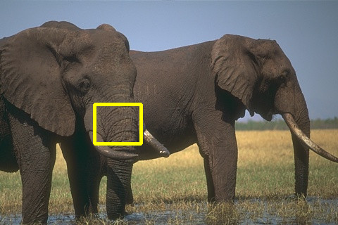
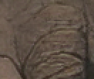
296059 from BSD100 (PSNR / LPIPS / PI) HR SRGAN [19] ENet [20] CX [21] EPSR2 [48] ($\infty$ / 0 / 2.3885) (28.96 / 0.1564 / 2.6015) (29.18 / 0.1432 / 2.8138) (28.57 / 0.1563 / 2.3492) (30.47 / 0.2046 /3.2575) EPSR3 [48] SuperSR [22] ESRGAN [22] S-RFN (Ours) PPON (Ours) (29.02 / 0.1911 /2.2666) (29.80 / 0.1703 /2.2913) (29.38 / 0.1333 / 2.3481) (31.40 / 0.3314 / 4.7222) (29.26 / 0.1305 / 2.5130)

Figure 18: A visual comparison with the state-of-the-art perceptual image SR algorithms.

We consider LPIPS [39] and PI [31] as our evaluation indices of perceptual image SR. As illustrated in Figure 18, we can see that the PI score of EPSR3 (2.2666) is even better than HR (2.3885), but EPSR3 shows unnatural and lacks proper texture and structure. When observing the results of ESRGAN and our PPON, their perception effect is superior to that of EPSR3, precisely in accordance with corresponding LPIPS values. From the results of S-RFN and PPON, it can be demonstrated that both PI and LPIPS have the ability to distinguish a blurring image. From the images of EPSR3, SuperSR, and ground-truth (HR), we can distinctly know that the lower PI value does not mean better image quality. Compared with the image generated by ESRGAN [22], it is evident that the proposed PPON gets a better visual effect with more structure information, corresponding to the lower LPIPS value. Because the PI (non-reference measure) is not sensitive to deformation through the experiment and cannot reflect the similarity with ground-truth, we take LPIPS as our primary perceptual measure and PI as a secondary metric.

Besides, we performed a MOS (mean opinion score) test to validate the effectiveness of our PPON further. Specifically, we collect $16$ raters to assign an integral score from $1$ (bad quality) to $5$ (excellent quality). To ensure the reliability of the results, we provide the raters with tests and original HR images simultaneously. The ground-truth images are set to $5$, and the raters then score the test images based on it. The average MOS results are shown in Table 9.

Table 9: Comparison of CX, ESRGAN, S-RFN, and PPON.

PIRM_Val	CX	ESRGAN	S-RFN(Ours)	PPON(Ours)
MOS	2.42	3.23	1.82	3.58
PSNR	25.41	25.18	28.63	26.20
SSIM	0.6747	0.6596	0.7913	0.6995

4.7 The influence of training patch size

Table 10: Quantitative evaluation of different perceptual-driven SR methods in LPIPS and PI. PPON_128 indicates the POBranch trained with $128\times 128$ image patches. The best and second best results are highlighted and underlined, respectively.

Method	PIRM_Val	PIRM_Test
	LPIPS / PI	LPIPS/ PI
ESRGAN [22]	0.1443 / 2.5550	0.1523 / 2.4356
PPON_128 (Ours)	0.1241 / 2.3026	0.1321 / 2.2080
PPON (Ours)	0.1194 / 2.2736	0.1273 / 2.1770

In ESRGAN [22], the authors mentioned that larger training patch sizes cost more training time and consume more computing resources. Thus, they used $192\times 192$ for PSNR-oriented methods and $128\times 128$ for perceptual-driven methods. In our main manuscript, we train the COBranch, SOBranch, and POBranch with $192\times 192$ image patches. Here, we further explore the influence of larger patches in the perceptual image generation stage.

It is important to note that the training perceptual-driven model requires more GPU memory and ore considerable computing resources than the PSNR-oriented model since the VGG model and discriminator need to be loaded during the training of the former. Therefore, larger patches ($192\times 192$) are hard to be used in optimizing ESRGAN [22] due to their large generator and discriminator to be updated. Thanks to our POBranch containing very few parameters, we employ $192\times 192$ training patches and achieve better results, as shown in Table 10. Concerning the discriminators, we illustrate them in Figure 19. For a fair comparison with the ESRGAN [22], we retrain our POBranch with $128\times 128$ patches and provide the results in Table 10.

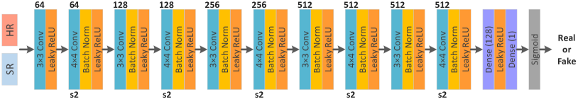
(a) Discriminator for $128\times 128$ training patches in PPON_128.

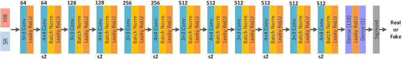
(b) Discriminator for $192\times 192$ training patches in PPON.

Figure 19: The network structure of the discriminators. The output size is scaled down by stride 2, and the parameter of LReLU is $0.2$.

5 Conclusion

In this paper, we propose a progressive perception-oriented network (PPON) for better perceptual image SR. Concretely, three branches are developed to learn the content, structure, and perceptual details, respectively. By exerting a stage-by-stage training scheme, we can steadily get promising results. It is worth mentioning that these three branches are not independent. A structure-oriented branch can exploit the extracted features and output images of the content-oriented branch. Extensive experiments on both traditional SR and perceptual SR demonstrate the effectiveness of our proposed PPON.

References

References

- [1] C. Dong, C. C. Loy, K. He, X. Tang, Learning a deep convolutional network for image super-resolution, in: ECCV, 2014, pp. 184–199.
- [2] C. Dong, C. C. Loy, K. He, X. Tang, Image super-resolution using deep convolutional networks, IEEE Transactions on Pattern Analysis and Machine Intelligence 38 (2) (2016) 295–307.
- [3] Y. Zhou, S. Kwong, W. Gao, X. Wang, A phase congruency based patch evaluator for complexity reduction in multi-dictionary based single-image super-resolution, Information Sciences 367-368 (2016) 337–353.
- [4] J. Luo, X. Sun, M. L. Yiu, L. Jin, X. Peng, Piecewise linear regression-based single image super-resolution via hadamard transform, Information Sciences 462 (2018) 315–330.
- [5] C. Dong, C. C. Loy, X. Tang, Accelerating the super-resolution convolutional neural network, in: ECCV, 2016, pp. 391–407.
- [6] J. Kim, J. K. Lee, K. M. Lee, Accurate image super-resolution using very deep convolutional networks, in: CVPR, 2016, pp. 1646–1654.
- [7] J. Kim, J. K. Lee, K. M. Lee, Deeply-recursive convolutional network for image super-resolution, in: CVPR, 2016, pp. 1637–1645.
- [8] W. Shi, J. Caballero, F. Huszár, J. Totz, A. P. Aitken, R. Bishop, D. Rueckert, Z. Wang, Real-time single image and video super-resolution using an efficient sub-pixel convolutional neural network, in: CVPR, 2016, pp. 1874–1883.
- [9] Y. Tai, J. Yang, X. Liu, Image super-resolution via deep recursive residual network, in: CVPR, 2017, pp. 3147–3155.
- [10] W.-S. Lai, J.-B. Huang, N. Ahuja, M.-H. Yang, Deep laplacian pyramid networks for fast and accurate super-resolution, in: CVPR, 2017, pp. 624–632.
- [11] B. Lim, S. Son, H. Kim, S. Nah, K. M. Lee, Enhanced deep residual networks for single image super-resolution, in: CVPR Workshop, 2017, pp. 136–144.
- [12] Y. Tai, J. Yang, X. Liu, C. Xu, Memnet: A persistent memory network for image restoration, in: ICCV, 2017, pp. 3147–3155.
- [13] T. Tong, G. Li, X. Liu, Q. Gao, Image super-resolution using dense skip connections, in: ICCV, 2017, pp. 4799–4807.
- [14] Z. Hui, X. Wang, X. Gao, Fast and accurate single image super-resolution via information distillation network, in: CVPR, 2018, pp. 723–731.
- [15] Y. Zhang, Y. Tian, Y. Kong, B. Zhong, Y. Fu, Residual dense network for image super-resolution, in: CVPR, 2018, pp. 2472–2481.
- [16] Y. Zhang, K. Li, K. Li, L. Wang, B. Zhong, Y. Fu, Image super-resolution using very deep residual channel attention networks, in: ECCV, 2018, pp. 286–301.
- [17] Z. Wang, A. Bovik, H. Sheikh, E. Simoncelli, Image quality assessment: from error visibility to structural similarity, IEEE Transactions on Image Processing 13 (4) (2004) 600–612.
- [18] J. Johnson, A. Alahi, F.-F. Li, Perceptual losses for real-time style transfer and super-resolution, in: ECCV, 2016, pp. 694–711.
- [19] C. Ledig, L. Theis, F. Huszar, J. Caballero, A. Cunningham, A. Acosta, A. Aitken, A. Tejani, J. Totz, Z. Wang, W. Shi, Photo-realistic single image super-resolution using a generative adversarial network, in: CVPR, 2017, pp. 4681–4690.
- [20] M. S. M. Sajjadi, B. Scholkopf, M. Hirsch, Enhancenet: Single image super-resolution through automated texture synthesis, in: ICCV, 2017, pp. 4491–4500.
- [21] R. Mechrez, I. Talmi, F. Shama, L. Zelnik-Manor, Maintaining natural image statistics with the contextual loss, in: ACCV, 2018.
- [22] X. Wang, K. Yu, S. Wu, J. Gu, Y. Liu, C. Dong, C. C. Loy, Y. Qiao, X. Tang, Esrgan: Enhanced super-resolution generative adversarial networks, in: ECCV Workshop, 2018.
- [23] K. Simonyan, A. Zisserman, Very deep convolutional networks for large-scale image recognition, in: ICLR, 2015.
- [24] I. Goodfellow, J. Pouget-Abadie, M. Mirza, B. Xu, D. Warde-Farley, S. Ozair, A. Courville, Y. Bengio, Generative adversarial nets, in: NIPS, 2014, pp. 2672–2680.
- [25] X. Wang, K. Yu, C. Dong, C. C. Loy, Recovering realistic texture in image super-resolution by deep spatial feature transform, in: CVPR, 2018, pp. 606–615.
- [26] S. Mehta, M. Rastegari, A. Caspi, L. Shapiro, H. Hajishirzi, Espnet: Efficient spatial pyramid of dilated convolutions for semantic segmentation, in: ECCV, 2018, pp. 552–568.
- [27] R. Timofte, E. Agustsson, L. V. Gool, M.-H. Yang, L. Zhang, et al, Ntire 2017 challenge on single image super-resolution: Methods and results, in: CVPR Workshop, 2017, pp. 1110–1121.
- [28] H. Liu, Z. Fu, J. Han, L. Shao, S. Hou, Y. Chu, Single image super-resolution using multi-scale deep encoder–decoder with phase congruency edge map guidance, Information Sciences 473 (2019) 44–58.
- [29] N. Ahn, B. Kang, K.-A. Sohn, Fast, accurate, and lightweight super-resolution with cascading residual network, in: ECCV, 2018, pp. 252–268.
- [30] S.-J. Park, H. Son, S. Cho, K.-S. Hong, S. Lee, Srfeat: Single image super-resolution with feature discrimination, in: ECCV, 2018, pp. 439–455.
- [31] Y. Blau, R. Mechrez, R. Timofte, T. Michaeli, L. Zelnik-Manor, 2018 pirm challenge on perceptual image super-resolution, in: ECCV Workshop, 2018.
- [32] Z. Wang, E. P. Simoncelli, A. C. Bovik, Multiscale structural similarity for image quality assessment, in: The Thrity-Seventh Asilomar Conference on Signals, Systems Computers, Vol. 2, 2003, pp. 1398–1402.
- [33] A. Jolicoeur-Martineau, The relativistic discriminator: a key element missing from standard gan, in: ICLR, 2019.
- [34] M. Bevilacqua, A. Roumy, C. Guillemot, M. line Alberi Morel, Low-complexity single-image super-resolution based on nonnegative neighbor embedding, in: BMVC, 2012, pp. 135.1–135.10.
- [35] R. Zeyde, M. Elad, M. Protter, On single image scale-up using sparse-representations, in: Curves and Surfaces, 2010, pp. 711–730.
- [36] D. Martin, C. Fowlkes, D. Tal, J. Malik, A database of human segmented natural images and its application to evaluating segmentation algorithms and measuring ecological statistics, in: CVPR, 2001, pp. 416–423.
- [37] J.-B. Huang, A. Singh, N. Ahuja, Single image super-resolution from transformed self-exemplars, in: CVPR, 2015, pp. 5197–5206.
- [38] Y. Matsui, K. Ito, Y. Aramaki, A. Fujimoto, T. Ogawa, T. Yamasaki, K. Aizawa, Sketch-based manga retrieval using manga109 dataset, Multimedia Tools and Applications 76 (20) (2017) 21811–21838.
- [39] R. Zhang, P. Isola, A. A. Efros, E. Shechtman, O. Wang, The unreasonable effectiveness of deep features as a perceptual metric, in: CVPR, 2018, pp. 586–595.
- [40] C. Ma, C.-Y. Yang, X. Yang, M.-H. Yang, Learning a no-reference quality metric for single-image super-resolution, Computer Vision and Image Understanding 158 (2017) 1–16.
- [41] A. Mittal, R. Soundararagan, A. C. Bovik, Making a ”completely blind” image quality analyzer, IEEE Signal Processing Letters 20 (3) (2013) 209–212.
- [42] D. P. Kingma, J. Ba, Adam: A method for stochastic optimization, in: ICLR, 2014.
- [43] K. Zhang, W. Zuo, L. Zhang, Learning a single convolutional super-resolution network for multiple degradations, in: CVPR, 2018, pp. 3262–3271.
- [44] M. Haris, G. Shakhnarovich, N. Ukita, Deep back-projection networks for super-resolution, in: CVPR, 2018, pp. 1664–1673.
- [45] J. Li, F. Fang, K. Mei, G. Zhang, Multi-scale residual network for image super-resolution, in: ECCV, 2018, pp. 517–532.
- [46] Z. Li, J. Yang, Z. Liu, X. Yang, G. Jeon, W. Wu, Feedback network for image super-resolution, in: CVPR, 2019, pp. 3867–3876.
- [47] T. Dai, J. Cai, Y. Zhang, S.-T. Xia, L. Zhang, Second-order attention network for single image super-resolution, in: CVPR, 2019, pp. 11065–11074.
- [48] S. Vasu, N. T. Madam, R. A.N., Analyzing perception-distortion tradeoff using enhanced perceptual super-resolution network, in: ECCV Workshop, 2018.
- [49] J. W. Soh, G. Y. Park, J. Jo, N. I. Cho, Natural and realistic single image super-resolution with explicit natural manifold discrimination, in: CVPR, 2019, pp. 8122–8131.
- [50] Y. Zhang, K. Li, K. Li, B. Zhong, Y. Fu, Residual non-local attention networks for image restoration, in: ICLR, 2019.