Medians in median graphs and their cube complexes in linear time¹

Abstract.

The median of a set of vertices $P$ of a graph $G$ is the set of all vertices $x$ of $G$ minimizing the sum of distances from $x$ to all vertices of $P$. In this paper, we present a linear time algorithm to compute medians in median graphs, improving over the existing quadratic time algorithm. We also present a linear time algorithm to compute medians in the $\ell_{1}$-cube complexes associated with median graphs. Median graphs constitute the principal class of graphs investigated in metric graph theory and have a rich geometric and combinatorial structure, due to their bijections with CAT(0) cube complexes and domains of event structures. Our algorithm is based on the majority rule characterization of medians in median graphs and on a fast computation of parallelism classes of edges ($\Theta$-classes or hyperplanes) via Lexicographic Breadth First Search (LexBFS). To prove the correctness of our algorithm, we show that any LexBFS ordering of the vertices of $G$ satisfies the following fellow traveler property of independent interest: the parents of any two adjacent vertices of $G$ are also adjacent. Using the fast computation of the $\Theta$-classes, we also compute the Wiener index (total distance) of $G$ in linear time and the distance matrix in optimal quadratic time.

1. Introduction

The median problem (also called the Fermat-Torricelli problem or the Weber problem) is one of the oldest optimization problems in Euclidean geometry [49]. The median problem can be defined for any metric space $(X,d)$: given a finite set $P\subset X$ of points with positive weights, compute the points $x$ of $X$ minimizing the sum of the distances from $x$ to the points of $P$ multiplied by their weights. The median problem in graphs is one of the principal models in network location theory [40, 71] and is equivalent to finding nodes with largest closeness centrality in network analysis [15, 16, 65]. It also occurs in social group choice as the Kemeny median. In the consensus problem in social group choice, given individual rankings of $d$ candidates one has to compute a consensual group decision. By the classical Arrow’s impossibility theorem, there is no consensus function satisfying natural “fairness” axioms. It is also well-known that the majority rule leads to Condorcet’s paradox, i.e., to the existence of cycles in the majority relation. In this respect, the Kemeny median [44, 45] is an important consensus function and corresponds to the median problem in graphs of permutahedra (the graph whose vertices are all $d!$ permutations of the candidates and whose edges are the pairs of permutations differing by adjacent transpositions). Other classical algorithmic problems related to distances are the diameter and center problems. Yet another such problem comes from chemistry and consists in the computation of the Wiener index of a graph. This is a topological index of a molecule, defined as the sum of the distances between all pairs of vertices in the associated chemical graph [76]. The Wiener index is closely related to the closeness centrality of a vertex in a graph, a quantity inversely proportional to the sum of all distances between the given vertex and all other vertices that has been frequently used in sociometry and the theory of social networks.

The median problem in Euclidean spaces cannot be solved in symbolic form [6], but can be solved numerically by Weiszfeld’s algorithm [75] and its convergent modifications (see e.g. [59]), and can be approximated in nearly linear time with arbitrary precision [29]. For the $\ell_{1}$-metric the median problem becomes easier and can be solved by the majority rule on coordinates, i.e., by taking as median a point whose $i$th coordinate is the median of the list of $i$th coordinates of the points of $P$. This kind of rule was used in [43] to define centroids of trees (which coincide with their medians [37, 71]) and can be viewed as an instance of the majority rule in social choice theory. For graphs with $n$ vertices, $m$ edges, and standard graph distance, the median problem can be trivially solved in $O(nm)$ time by solving the All Pairs Shortest Paths (APSP) problem. One may ask if APSP is necessary to compute the median. However, by [1] APSP and median problem are equivalent under subcubic reductions. It was also shown in [2] that computing the medians of sparse graphs in subquadratic time refutes the HS (Hitting Set) conjecture. It was also noted in [20] that computing the Wiener index of a sparse graph in subquadratic time will refute the Exponential time (SETH) hypothesis. Note also that computing the Kemeny median is NP-hard [33] if the input is the list of individual preferences.

In this paper, we show that the medians in median graphs can be computed in optimal $O(m)$ time (i.e., without solving APSP). Median graphs are the graphs in which each triplet $u,v,w$ of vertices has a unique median, i.e., a vertex metrically lying between $u$ and $v$, $v$ and $w$, and $w$ and $u$. They originally arise in universal algebra [4, 18] and their properties have been first investigated in [53, 57]. It was shown in [26, 62] that the cube complexes of median graphs are exactly the CAT(0) cube complexes, i.e., cube complexes of global non-positive curvature. CAT(0) cube complexes, introduced and nicely characterized in [38] in a local-to-global way, are now one of the principal objects of investigation in geometric group theory [67]. Median graphs also occur in Computer Science: by [3, 13] they are exactly the domains of event structures (one of the basic abstract models of concurrency) [58] and median-closed subsets of hypercubes are exactly the solution sets of 2-SAT formulas [56, 68]. The bijections between median graphs, CAT(0) cube complexes, and event structures have been used in [21, 22, 27] to disprove three conjectures in concurrency [64, 72, 73]. Finally, median graphs, viewed as median closures of sets of vertices of a hypercube, contain all most parsimonious (Steiner) trees [12] and as such have been extensively applied in human genetics. For a survey on median graphs and their connections with other discrete and geometric structures, see the books [41, 48], the surveys [10, 47], and the paper [23].

As we noticed, median graphs have strong geometric and metric properties. For the median problem, the concept of $\Theta$-classes is essential. Two edges of a median graph $G$ are called opposite if they are opposite in a common square of $G$. The equivalence relation $\Theta$ is the reflexive and transitive closure of this oppositeness relation. Each equivalence class of $\Theta$ is called a $\Theta$-class ($\Theta$-classes correspond to hyperplanes in CAT(0) cube complexes [66] and to events in event structures [58]). Removing the edges of a $\Theta$-class, the graph $G$ is split into two connected components which are convex and gated. Thus they are called halfspaces of $G$. The convexity of halfspaces implies via [32] that any median graph $G$ isometrically embeds into a hypercube of dimension equals to the number $q$ of $\Theta$-classes of $G$.

Our results and motivation

In this paper, we present a linear time algorithm to compute medians in median graphs and in associated $\ell_{1}$-cube complexes. Our main motivation and technique stem from the majority rule characterization of medians in median graphs and the unimodality of the median function [8, 70]. Even if the majority rule is simple to state and is a commonly approved consensus method, its algorithmic implementation is less trivial if one has to avoid the computation of the distance matrix. On the other hand, the unimodality of the median function implies that one may find the median set by using local search. More generally, consider a partial orientation of the input median graph $G$, where an edge $uv$ is transformed into the arc $\overrightarrow{uv}$ iff the median function at $u$ is larger than the median function at $v$ (in case of equality we do not orient the edge $uv$). Then the median set is exactly the set of all the sinks in this partial orientation of $G$. Therefore, it remains to compare for every edge $uv$ the median function at $u$ and at $v$ in constant time. For this we use the partition of the edge-set of a median graph $G$ into $\Theta$-classes and; for every $\Theta$-class, the partition of the vertex-set of $G$ into complementary halfspaces. It is easy to notice that all edges of the same $\Theta$-class are oriented in the same way because for any such edge $uv$ the difference between the median functions at $u$ and at $v$, respectively, can be expressed as the sum of weights of all vertices in the same halfspace as $v$ minus the sum of weights of all vertices in the same halfspace as $u$.

Our main technical contribution is a new method for computing the $\Theta$-classes of a median graph $G$ with $n$ vertices and $m$ edges in linear $O(m)$ time. For this, we prove that Lexicographic Breadth First Search (LexBFS) [63] produces an ordering of the vertices of $G$ satisfying the following fellow traveler property: for any edge $uv$, the parents of $u$ and $v$ are adjacent. With the $\Theta$-classes of $G$ at hand and the majority rule for halfspaces, we can compute the weights of halfspaces of $G$ in optimal time $O(m)$, leading to an algorithm of the same complexity for computing the median set. We adapt our method to compute in linear time the median of a finite set of points in the $\ell_{1}$-cube complex associated with $G$. We also show that this method can be applied to compute the Wiener index in optimal $O(m)$ time and the distance matrix of $G$ in optimal $O(n^{2})$ time.

In all previous results we assumed that the input of the problem is given by the median graph or its cube complex, together with the set of terminals and their weights. However, analogously to the Kemeny median problem, the median problem in a median graph $G$ can be defined in a more compact way. We mentioned above that median graphs are exactly the domains of configurations of event structures and the solution sets of 2-SAT formulas (with no equivalent variables). The underlying event structure or the underlying 2-SAT formula provide a much more compact (but implicit) description of the median graph $G$. Therefore, we can formulate a median problem by supposing that the input is a set of configurations of an event structure and their weights. The goal is to compute a configuration minimizing the sum of the weighted (Hamming) distances to the terminal-configurations. Thanks to the majority rule, we show that this median problem can be efficiently solved in the size of the input. Finally, we suppose that the input is an event structure and the goal is to compute a configuration minimizing the sum of distances to all configurations. We show that this problem is $\#$P-hard. For this we establish a direct correspondence between event structures and 2-SAT formulas and we use a result by Feder [36] that an analogous median problem for 2-SAT formulas is $\#$P-hard.

Related work

The study of the median problem in median graphs originated in [8, 70] and continued in [7, 51, 54, 55, 61]. Using different techniques and extending the majority rule for trees [37], the following majority rule has been established in [8, 70]: a halfspace $H$ of a median graph $G$ contains at least one median iff $H$ contains at least one half of the total weight of $G$; moreover, the median of $G$ coincides with the intersection of halfspaces of $G$ containing strictly more than half of the total weight. It was shown in [70] that the median function of a median graph is weakly convex (an analog of a discrete convex function). This convexity property characterizes all graphs in which all local medians are global [9]. A nice axiomatic characterization of medians of median graphs via three basic axioms has been obtained in [55]. More recently, [61] characterized median graphs as closed Condorcet domains, i.e., as sets of linear orders with the property that, whenever the preferences of all voters belong to the set, their majority relation has no cycles and also belongs to the set. Below we will show that the median graphs are the bipartite graphs in which the medians are characterized by the majority rule.

Prior to our work, the best algorithm to compute the $\Theta$-classes of a median graph $G$ has complexity $O(m\log n)$ [39]. It was used in [39] to recognize median graphs in subquadratic time. The previous best algorithm for the median problem in a median graph $G$ with $n$ vertices and $q$ $\Theta$-classes has complexity $O(qn)$ [7] which is quadratic in the worst case. Indeed $q$ may be linear in $n$ (as in the case of trees) and is always at least $d(\sqrt[d]{n}-1)$ as shown below ($d$ is the largest dimension of a hypercube which is an induced subgraph of $G$). Additionally, [7] assumes that an isometric embedding of $G$ in a $q$-hypercube is given. The description of such an embedding has already size $O(qn)$. The $\Theta$-classes of a median graph $G$ correspond to the coordinates of the smallest hypercube in which $G$ isometrically embeds (this is called the isometric dimension of $G$ [41]). Thus one can define $\Theta$-classes for all partial cubes, i.e., graphs isometrically embeddable into hypercubes. An efficient computation (in $O(n^{2})$ time) of all $\Theta$-classes was the main step of the $O(n^{2})$ algorithm of [34] for recognizing partial cubes. The fellow-traveler property (which is essential in our computation of $\Theta$-classes) is a notion coming from geometric group theory [35] and is a main tool to prove the (bi)automaticity of a group. In a slightly stronger form it allows to establish the dismantlability of graphs (see [19, 25, 26] for examples of classes of graphs in which a fellow traveler order was obtained by BFS or LexBFS). LexBFS has been used to solve optimally several algorithmic problems in different classes of graphs, in particular for their recognition (for a survey, see [31]).

Cube complexes of median graphs with $\ell_{1}$-metric have been investigated in [74]. The same complexes but endowed with the $\ell_{2}$-metric are exactly the CAT(0) cube complexes. As we noticed above, they are of great importance in geometric group theory [67]. The paper [17] established that the space of trees with a fixed set of leaves is a CAT(0) cube complex. A polynomial-time algorithm to compute the $\ell_{2}$-distance between two points in this space was proposed in [60]. This result was recently extended in [42] to all CAT(0) cube complexes. A convergent numerical algorithm for the median problem in CAT(0) spaces was given in [5].

Finally, for an extensive bibliography on Wiener index in graphs, see [41, 46]. The Wiener index of a tree can be computed in linear time [52]. Using this and the fact that benzenoids (i.e., subgraphs of the hexagonal grid bounded by a simple curve) isometrically embed in the product of three trees, [28] proposed a linear time algorithm for the Wiener index of benzenoids. Finally, in a recent breakthrough [20], a subquadratic algorithm for the Wiener index and the diameter of planar graphs was presented.

(a)

(b)

Figure 1. Two median graphs, the second one (denoted by $D$) will be our running example.

2. Preliminaries

All graphs $G=(V,E)$ in this paper are finite, undirected, simple, and connected; $V$ is the vertex-set and $E$ is the edge-set of $G$. We write $u\sim v$ if $u,v\in V$ are adjacent. The distance $d(u,v)=d_{G}(u,v)$ between two vertices $u$ and $v$ is the length of a shortest $(u,v)$-path, and the interval $I(u,v)=\{x\in V:d(u,x)+d(x,v)=d(u,v)\}$ consists of all the vertices on shortest $(u,v)$–paths. A set $H$ (or the subgraph induced by $H$) is convex if $I(u,v)\subseteq H$ for any two vertices $u,v$ of $H$; $H$ is a halfspace if $H$ and $V\setminus H$ are convex. Finally, $H$ is gated if for every vertex $v\in V$, there exists a (unique) vertex $v^{\prime}\in V(H)$ (the gate of $v$ in $H$) such that for all $u\in V(H)$, $v^{\prime}\in I(u,v)$. The $k$-dimensional hypercube $Q_{k}$ has all subsets of $\{1,\ldots,k\}$ as the vertex-set and $A\sim B$ iff $|A\triangle B|=1$. A graph $G$ is called median if $I(x,y)\cap I(y,z)\cap I(z,x)$ is a singleton for each triplet $x,y,z$ of vertices; this unique intersection vertex $m(x,y,z)$ is called the median of $x,y,z$. Median graphs are bipartite and do not contain induced $K_{2,3}$. The dimension $d=\dim(G)$ of a median graph $G$ is the largest dimension of a hypercube of $G$. In $G$, we refer to the $4$-cycles as squares, and the hypercube subgraphs as cubes.

A map $w:V\rightarrow\mathbb{R}^{+}\cup\{0\}$ is called a weight function. For a vertex $v\in V$, $w(v)$ denotes the weight of $v$ (for a set $S\subseteq V$, $w(S)=\sum_{x\in S}w(x)$ denotes the weight of $S$). Then $F_{w}(x)=\sum_{v\in V}w(v)d(x,v)$ is called the median function of the graph $G$ and a vertex $x$ minimizing $F_{w}$ is called a median vertex of $G$. Finally, $\operatorname*{Med}_{w}(G)=\{x\in V:x\mbox{ is a median of }G\}$ is called the median set (or simply, the median) of $G$ with respect to the weight function $w$. The Wiener index $W(G)$ (called also the total distance) of a graph $G$ is the sum of all pairwise distances between the vertices of $G$. For a weight function $w$, the Wiener index of $G$ is the sum $W_{w}(G)=\sum_{u,v\in V}w(u)w(v)d(u,v)$.

3. Facts about median graphs

We recall the principal properties of median graphs used in the algorithms. Some of those results are a part of folklore for the people working in metric graph theory and some other results can be found in the papers [53, 54] by Mulder. For readers convenience, we provide the proofs (sometimes different from the original proofs) of all those results in the Appendix.

From now on, $G=(V,E)$ is a median graph with $n$ vertices and $m$ edges. The first three properties follow from the definition.

Lemma 3.1 (Quadrangle Condition).

For any vertices $u,v,w,z$ of $G$ such that $v,w\sim z$ and $d(u,v)=d(u,w)=d(u,z)-1=k$, there is a unique vertex $x\sim v,w$ such that $d(u,x)=k-1$.

Lemma 3.2 (Cube Condition).

Any three squares of $G$, pairwise intersecting in three edges and all three intersecting in a single vertex, belong to a 3-dimensional cube of $G$.

Lemma 3.3 (Convex=Gated).

A subgraph of $G$ is convex if and only if it is gated.

Two edges $uv$ and $u^{\prime}v^{\prime}$ of $G$ are in relation $\Theta_{0}$ if $uvv^{\prime}u^{\prime}$ is a square of $G$ and $uv$ and $u^{\prime}v^{\prime}$ are opposite edges of this square. Let $\Theta$ denote the reflexive and transitive closure of $\Theta_{0}$. Denote by $E_{1},\ldots,E_{q}$ the equivalence classes of $\Theta$ and call them $\Theta$-classes (see Fig. 2(a)).

Lemma 3.4 (​​[53])(Halfspaces and $\Theta$-classes).

For any $\Theta$-class $E_{i}$ of $G$, the graph $G_{i}=(V,E\setminus E_{i})$ consists of exactly two connected components $H^{\prime}_{i}$ and $H^{\prime\prime}_{i}$ that are halfspaces of $G$; all halfspaces of $G$ have this form. If $uv\in E_{i}$, then $H^{\prime}_{i}$ and $H^{\prime\prime}_{i}$ are the subgraphs of $G$ induced by $W(u,v)=\{x\in V:d(u,x)<d(v,x)\}$ and $W(v,u)=\{x\in V:d(v,x)<d(u,x)\}$.

By [32], $G$ is a partial cube, (i.e., isometrically embeds into an hypercube) iff $G$ is bipartite and $W(u,v)$ is convex for any edge $uv$ of $G$. Consequently, we obtain the following corollary.

Corollary 3.5.

$G$ isometrically embeds into a hypercube of dimension equals to the number $q$ of $\Theta$-classes of $G$.

Lemma 3.6.

Each convex subgraph $S$ of $G$ is the intersection of all halfspaces containing $S$.

Two $\Theta$-classes $E_{i}$ and $E_{j}$ are crossing if each halfspace of the pair $\{H^{\prime}_{i},H^{\prime\prime}_{i}\}$ intersects each halfspace of the pair $\{H^{\prime}_{j},H^{\prime\prime}_{j}\}$; otherwise, $E_{i}$ and $E_{j}$ are called laminar.

Lemma 3.7 (Crossing $\Theta$-classes).

Any vertex $v\in V(G)$ and incident edges $vv_{1}\in E_{1},\ldots,vv_{k}\in E_{k}$ belong to a single cube of $G$ if and only if $E_{1},\ldots,E_{k}$ are pairwise crossing.

The boundary $\partial H^{\prime}_{i}$ of a halfspace $H^{\prime}_{i}$ is the subgraph of $H^{\prime}_{i}$ induced by all vertices $v^{\prime}$ of $H^{\prime}_{i}$ having a neighbor $v^{\prime\prime}$ in $H^{\prime\prime}_{i}$. A halfspace $H^{\prime}_{i}$ of $G$ is peripheral if $\partial H^{\prime}_{i}=H^{\prime}_{i}$ (See Fig. 2(b)).

Lemma 3.8 (Boundaries).

For any $\Theta$-class $E_{i}$ of $G$, $\partial H^{\prime}_{i}$ and $\partial H^{\prime\prime}_{i}$ are isomorphic and gated.

From now on, we suppose that $G$ is rooted at an arbitrary vertex $v_{0}$ called the basepoint. For any $\Theta$-class $E_{i}$, we assume that $v_{0}$ belongs to the halfspace $H^{\prime\prime}_{i}$. Let $d(v_{0},H^{\prime}_{i})=\min\{d(v_{0},x):x\in H^{\prime}_{i}\}$. Since $H^{\prime}_{i}$ is gated, the gate of $v_{0}$ in $H^{\prime}_{i}$ is the unique vertex of $H^{\prime}_{i}$ at distance $d(v_{0},H^{\prime}_{i})$ from $v_{0}$. Since median graphs are bipartite, the choice of $v_{0}$ defines a canonical orientation of the edges of $G$: $uv\in E$ is oriented from $u$ to $v$ (notation $\overrightarrow{uv}$) if $d(v_{0},u)<d(v_{0},v)$. Let $\overrightarrow{G}_{v_{0}}$ denote the resulting oriented pointed graph.

Lemma 3.9 (​​[54])(Peripheral Halfspaces).

Any halfspace $H^{\prime}_{i}$ maximizing $d(v_{0},H^{\prime}_{i})$ is peripheral.

(a)

(b)

(c)

Figure 2.  (a) In dashed, the $\Theta$-class $E_{i}$ of $D$, its two complementary halfspaces $H^{\prime}_{i}$ and $H^{\prime\prime}_{i}$ and their boundaries $\partial H_{i}^{\prime}$ and $\partial H_{i}^{\prime\prime}$, (b) two peripheral halfspaces of $D$, and (c) a LexBFS ordering of $D$.

For a vertex $v$, all vertices $u$ such that $\overrightarrow{uv}$ is an edge of $\overrightarrow{G}_{v_{0}}$ are called predecessors of $v$ and are denoted by $\Lambda(v)$. Equivalently, $\Lambda(v)$ consists of all neighbors of $v$ in the interval $I(v_{0},v)$. A median graph $G$ satisfies the downward cube property if any vertex $v$ and all its predecessors $\Lambda(v)$ belong to a single cube of $G$.

Lemma 3.10 (​​[53])(Downward Cube Property).

$G$ satisfies the downward cube property.

Lemma 3.10 immediately implies the following upper bound on the number of edges of $G$:

Corollary 3.11.

If $G$ has dimension $d$, then $m\leq dn\leq n\log n$.

We give a sharp lower bound on the number $q$ of $\Theta$-classes, which is new to our knowledge.

Proposition 3.12.

If $G$ has $q$ $\Theta$-classes and dimension $d$, then $q\geq d(\sqrt[d]{n}-1)$. This lower bound is realized for products of $d$ paths of length $\sqrt[d]{n}-1$.

Proof.

Let $\Gamma(G)$ be the crossing graph $\Gamma(G)$ of $G$: $V(\Gamma(G))$ is the set of $\Theta$-classes of $G$ and two $\Theta$-classes are adjacent in $\Gamma(G)$ if they are crossing. Note that $|V(\Gamma(G))|=q$. Let $X(\Gamma(G))$ be the clique complex of $\Gamma(G)$. By the characterization of median graphs among ample classes [11, Proposition 4], the number of vertices of $G$ is equal to the number $|X(\Gamma(G))|$ of simplices of $X(\Gamma(G))$. Since $G$ is of dimension $d$, by [11, Proposition 4], $\Gamma(G)$ does not contain cliques of size $d+1$. By Zykov’s theorem [79] (see also [78]), the number of $k$-simplices in $X(\Gamma(G))$ is at most $\binom{d}{k}\left(\frac{q}{d}\right)^{k}$. Hence $n=|V(G)|=|X(\Gamma(G))|\leq\sum_{k=0}^{d}\binom{d}{k}\left(\frac{q}{d}\right)^{k}=\left(1+\frac{q}{d}\right)^{d}$ and thus $q\geq d(\sqrt[d]{n}-1)$. Let now $G$ be the Cartesian product of $d$ paths of length $(\sqrt[d]{n}-1)$. Then $G$ has $(\sqrt[d]{n}-1+1)^{d}=n$ vertices and $d(\sqrt[d]{n}-1)$ $\Theta$-classes (each $\Theta$-class of $G$ corresponds to an edge of one of factors). ∎

4. Computation of the $\Theta$-classes

In this section we describe two algorithms to compute the $\Theta$-classes of a median graph $G$: one runs in time $O(dm)$ and uses BFS, and the other runs in time $O(m)$ and uses LexBFS.

4.1. $\Theta$-classes via BFS

The Breadth-First Search (BFS) refines the basepoint order and defines the same orientation $\overrightarrow{G}_{v_{0}}$ of $G$. BFS uses a queue $Q$ and the insertion in $Q$ defines a total order $<$ on the vertices of $G$: $x<y$ iff $x$ is inserted in $Q$ before $y$. When a vertex $u$ arrives at the head of $Q$, it is removed from $Q$ and all not yet discovered neighbors $v$ of $u$ are inserted in $Q$; $u$ becomes the parent $f(v)$ of $v$; for any vertex $v\neq v_{0}$, $f(v)$ is the smallest predecessor of $v$. The arcs $\overrightarrow{f(v)v}$ define the BFS-tree of $G$. For each vertex $v$, BFS produces the list $\Lambda(v)$ of predecessors of $v$ ordered by $<$; denote this ordered list by $\Lambda_{<}(v)$. By Lemma 3.10, each list $\Lambda_{<}(v)$ has size at most $d:=\dim(G)$. Notice also that the total order $<$ on vertices of $G$ give raise to a total order on the edges of $G$: for two edges $uv$ and $u^{\prime}v^{\prime}$ with $u<v$ and $u^{\prime}<v^{\prime}$ we have $uv<u^{\prime}v^{\prime}$ if and only if $u<u^{\prime}$ or if $u=u^{\prime}$ and $v<v^{\prime}$.

Now we show how to use a BFS rooted at $v_{0}$ to compute, for each edge $uv$ of a median graph $G$, the unique $\Theta$-class $E(uv)$ containing the edge $uv$. Suppose that $uv$ is oriented by BFS from $u$ to $v$, i.e., $d(v_{0},u)<d(v_{0},v)$. There are only two possibilities: either the edge $uv$ is the first edge of the $\Theta$-class $E(uv)$ discovered by BFS or the $\Theta$-class of $uv$ already exists. The following lemma shows how to distinguish between these two cases:

Lemma 4.1.

An edge $uv\in E_{i}$ with $d(v_{0},u)<d(v_{0},v)$ is the first edge of a $\Theta$-class $E_{i}$ iff $u$ is the unique predecessor of $v$, i.e., $\Lambda_{<}(v)=\{u\}$.

Proof.

First let $uv$ be the first edge of $E_{i}$ discovered by BFS. Since $H^{\prime}_{i}$ is gated, $v$ is the gate of $v_{0}$ in $H^{\prime}_{i}$ and $u$ is the unique neighbor of $v$ in $H^{\prime\prime}_{i}$. We assert that $u$ is the unique neighbor of $v$ in $I(v_{0},v)$. Suppose $I(v_{0},v)$ contains a second neighbor $u^{\prime\prime}$ of $v$. Since $v$ is the gate of $v_{0}$ in $H^{\prime}_{i}$ and $u^{\prime\prime}$ is closer to $v_{0}$ than $v$, $u^{\prime\prime}$ necessarily belongs to $H^{\prime\prime}_{i}$, a contradiction with the uniqueness of $u$. Conversely, suppose that $v$ has only $u$ as a neighbor in $I(v_{0},v)$ but $uv$ is not the first edge of $E_{i}$ with respect to the BFS. This implies that the gate $x$ of $v_{0}$ in $H^{\prime}_{i}$ is different from $v$. Let $u^{\prime}$ be a neighbor of $v$ in $I(x,v)$ and note that $I(x,v)\subseteq I(v_{0},v)$. Since $v,x\in H^{\prime}_{i}$ and $H^{\prime}_{i}$ is convex, $u^{\prime}$ belongs to $H^{\prime}_{i}$. Since $u$ belongs to $H^{\prime\prime}_{i}$, we conclude that $u$ and $u^{\prime}$ are two different neighbors of $v$ in $I(v_{0},v)$, a contradiction. ∎

If $uv$ is not the first edge of its $\Theta$-class, the following lemma shows how to find its $\Theta$-class:

Lemma 4.2.

Let $uv$ be an edge of a median graph with $u\in\Lambda_{<}(v)$. If $v$ has a second predecessor $v^{\prime}$, then there exists a square $u^{\prime}uvv^{\prime}$ in which $uv$ and $u^{\prime}v^{\prime}$ are opposite edges and $u^{\prime}\in\Lambda_{<}(u)\cap\Lambda_{<}(v^{\prime})$.

Proof.

Indeed, by the quadrangle condition, the vertices $u$ and $v^{\prime}$ have a unique common neighbor $u^{\prime}$ such that $u^{\prime}uvv^{\prime}$ is a square of $G$ and $u^{\prime}$ is closer to $v_{0}$ than $u$ and $v^{\prime}$. Consequently, $u^{\prime}\in\Lambda_{<}(u)\cap\Lambda_{<}(v^{\prime})$ and $uv$ and $u^{\prime}v^{\prime}$ are opposite edges of $u^{\prime}uvv^{\prime}$. ∎

From Lemmas 4.1 and 4.2 we deduce the following algorithm for computing the $\Theta$-classes of $G$. First, run a BFS and return a BFS-ordering of the vertices and edges of $G$ and the ordered lists $\Lambda_{<}(v),v\in V$. Then consider the edges of $G$ in the BFS-order. Pick a current edge $uv$ and suppose that $u\in\Lambda_{<}(v)$. If $\Lambda_{<}(v)=\{u\}$, by Lemma 4.1 $uv$ is the first edge of its $\Theta$-class, thus create a new $\Theta$-class $E_{i}$ and insert $uv$ in $E_{i}$. Otherwise, if $v$ has a second predecessor $v^{\prime}$, then traverse the ordered lists $\Lambda_{<}(u)$ and $\Lambda_{<}(v^{\prime})$ to find their unique common predecessor $u^{\prime}$ (which exists by Lemma 4.2). Then insert the edge $uv$ in the $\Theta$-class of the edge $u^{\prime}v^{\prime}$. Since the two sorted lists $\Lambda_{<}(u)$ and $\Lambda_{<}(v^{\prime})$ are of size at most $d$, their intersection (that contains only $u^{\prime}$) can be computed in time $O(d)$, and thus the $\Theta$-class of each edge $uv$ of $G$ can be computed in $O(d)$ time. Consequently, we obtain:

Proposition 4.3.

The $\Theta$-classes of a median graph $G$ with $n$ vertices, $m$ edges, and dimension $d$ can be computed in $O(dm)=O(d^{2}n)$ time.

4.2. $\Theta$-classes via LexBFS

The Lexicographic Breadth-First Search (LexBFS), proposed in [63], is a refinement of BFS. In BFS, if $u$ and $v$ have the same parent, then the algorithm order them arbitrarily. Instead, the LexBFS chooses between $u$ and $v$ by considering the ordering of their second-earliest predecessors. If only one of them has a second-earliest predecessor, then that one is chosen. If both $u$ and $v$ have the same second-earliest predecessor, then the tie is broken by considering their third-earliest predecessor, and so on (See Fig. 2(c)). The LexBFS uses a set partitioning data structure and can be implemented in linear time [63]. In median graphs, the next lemma shows that it suffices to consider only the earliest and second-earliest predecessors, leading to a simpler implementation of LexBFS:

Lemma 4.4.

If $u$ and $v$ are two vertices of a median graph $G$, then $|\Lambda(u)\cap\Lambda(v)|\leq 1$.

Proof.

Let $x,x^{\prime}$ be two distinct predecessors of $u$ and $v$. Since $x,x^{\prime}\in\Lambda(u)\cap\Lambda(v)$, we have $d(v_{0},u)=d(v_{0},v)=d(v_{0},x)+1=d(v_{0},x^{\prime})+1=k+1$. By Lemma 3.1, there is a vertex $y\sim x,x^{\prime}$ at distance $k-1$ from $v_{0}$. But then $x,x^{\prime},u,v,y$ induce a forbidden $K_{2,3}$. ∎

A graph $G$ satisfies the fellow-traveler property if for any LexBFS ordering of the vertices of $G$, for any edge $uv$ with $v_{0}\notin\{u,v\}$, the parents $f(u)$ and $f(v)$ are adjacent.

Theorem 4.5.

Any median graph $G$ satisfies the fellow-traveler property.

Proof.

Let $<$ be an arbitrary LexBFS order of the vertices of $G$ and $f$ be its parent map. Since any LexBFS order is a BFS order, $<$ and $f$ satisfy the following properties of BFS:

1. if $u<v$, then $f(u)\leq f(v)$;

2. if $f(u)<f(v)$, then $u<v$;

3. if $v\neq v_{0}$, then $f(v)=\min_{<}\{u:u\sim v\}$;

4. if $u<v$ and $v\sim f(u)$, then $f(v)=f(u)$.

Notice also the following simple but useful property:

Lemma 4.6.

If $abcd$ is a square of $G$ with $d(v_{0},c)=k$, $d(v_{0},b)=d(v_{0},d)=k+1,d(v_{0},a)=k+2$ and $f(a)=b$, and the edge $ad$ satisfies the fellow-traveler property, then $f(d)=c$.

Proof.

By the fellow traveler property, $f(d)\sim f(a)=b$. If $f(d)\neq c$, then $a,b,c,d,f(d)$ induce a forbidden $K_{2,3}$. ∎

(a)

(b)

(c)

(d)

(e)

(f)

(g)

(h)

(i)

Figure 3. Animated proof of Theorem 4.5.

We prove the fellow-traveler property by induction on the total order on the edges of $G$ defined by $<$. The proof is illustrated by several figures (the arcs of the parent map are represented in bold). We use the following convention: all vertices having the same distance to the basepoint $v_{0}$ will be labeled by the same letter but will be indexed differently; for example, $w_{1}$ and $w_{2}$ are two vertices having the same distance to $v_{0}$.

Suppose by way of contradiction that $e=u_{1}v_{3}$ with $v_{3}<u_{1}$ is the first edge in the order $<$ such that the parents $f(u_{1})$ and $f(v_{3})$ of $u_{1}$ and $v_{3}$ are not adjacent. Then necessarily $f(u_{1})\neq v_{3}$. Set $v_{1}=f(u_{1})$ and $w_{3}=f(v_{3})$ (Fig. 3(a)). Since $d(v_{0},v_{1})=d(v_{0},v_{3})$ and $u_{1}\sim v_{1},v_{3}$, by the quadrangle condition $v_{1}$ and $v_{3}$ have a common neighbor at distance $d(v_{0},v_{1})-1$ from $v_{0}$. This vertex cannot be $w_{3}$, otherwise $f(u_{1})$ and $f(v_{3})$ would be adjacent. Therefore there is a vertex $w_{4}\sim v_{1},v_{3}$ at distance $d(v_{0},v_{1})-1$ from $v_{0}$ (Fig. 3(b)). By induction hypothesis, the parent $x_{3}=f(w_{4})$ of $w_{4}$ is adjacent to $w_{3}=f(v_{3})$. Since $u_{1}\sim v_{1}=f(u_{1}),v_{3}$ and $v_{3}\sim w_{3}=f(v_{3}),w_{4}$, by (BFS3) we conclude that $v_{1}<v_{3}$ and $w_{3}<w_{4}$. By (BFS2), $f(v_{1})\leq f(v_{3})$, whence $f(v_{1})\leq w_{3}$ and since $f(v_{1})\neq f(v_{3})$ (otherwise, $f(u_{1})\sim f(v_{3})$), we deduce that $f(v_{1})<w_{3}<w_{4}$. Hence $f(v_{1})\neq w_{4}$. Set $w_{1}=f(v_{1})$. By the induction hypothesis, $f(v_{1})=w_{1}$ is adjacent to $f(w_{4})=x_{3}$ (Fig. 3(c)). By the cube condition applied to the squares $w_{4}v_{1}w_{1}x_{3}$, $w_{4}v_{1}u_{1}v_{3}$, and $w_{4}v_{3}w_{3}x_{3}$ there is a vertex $v_{2}$ adjacent to $u_{1}$, $w_{1}$, and $w_{3}$. Since $u_{1}\sim v_{2}$ and $f(u_{1})=v_{1}$, by (BFS3) we obtain $v_{1}<v_{2}$. Since $v_{2}$ is adjacent to $w_{1}$ and $w_{1}=f(v_{1})$, by (BFS4) we obtain $f(v_{2})=f(v_{1})=w_{1}$, and by (BFS2), $v_{2}<v_{3}$. Since $f(v_{2})=w_{1}$, by Lemma 4.6 for $v_{2}w_{1}x_{3}w_{3}$, we obtain $f(w_{3})=x_{3}$ (Fig. 3(d)). Since $v_{1}<v_{2}$, $f(v_{1})=f(v_{2})=w_{1}$, and $v_{2}\sim w_{1},w_{3}$, by LexBFS $v_{1}$ is adjacent to a predecessor different from $w_{1}$ and smaller than $w_{3}$. Since $w_{3}<w_{4}$, this predecessor cannot be $w_{4}$. Denote by $w_{2}$ the second smallest predecessor of $v_{1}$ (Fig. 3(e)) and note that $w_{1}<w_{2}<w_{3}<w_{4}$.

By the quadrangle condition, $w_{2}$ and $w_{4}$ are adjacent to a vertex $x_{5}$, which is necessarily different from $x_{3}$ because $G$ is $K_{2,3}$-free. By the induction hypothesis, $f(w_{2})$ and $f(v_{1})=w_{1}$ are adjacent. Then $f(w_{2})\neq x_{3},x_{5}$, otherwise we obtain a forbidden $K_{2,3}$. Set $f(w_{2})=x_{2}$. Analogously, $f(x_{5})=y_{5}$ and $f(w_{2})=x_{2}$ are adjacent as well as $f(x_{5})=y_{5}$ and $f(w_{4})=x_{3}$ (Fig. 3(f)). By (BFS1), $x_{2}=f(w_{2})<f(w_{3})=x_{3}$ and by (BFS3), $x_{3}=f(w_{4})<x_{5}$. Since $w_{3}<w_{4}$ with $f(w_{3})=f(w_{4})$ and $w_{4}$ is adjacent to $x_{5}$, by LexBFS $w_{3}$ must have a predecessor different from $x_{3}$ and smaller than $x_{5}$. This vertex cannot be $x_{2}$ by (BFS3) since $f(w_{3})=x_{3}$. Denote this predecessor of $w_{3}$ by $x_{4}$ and observe that $x_{2}<x_{3}<x_{4}<x_{5}$. By the induction hypothesis, the parent of $x_{4}$ is adjacent to $f(w_{3})=x_{3}$. Let $y_{4}=f(x_{4})$.

If $y_{4}=y_{5}$, applying the cube condition to the squares $x_{3}w_{3}x_{4}y_{5}$, $x_{3}w_{4}x_{5}y_{5}$, and $x_{3}w_{4}v_{3}w_{3}$ we find a vertex $w$ adjacent to $x_{4}$, $v_{3}$, and $x_{5}$. Applying the cube condition to the squares $w_{4}v_{3}wx_{5}$, $w_{4}v_{1}w_{2}x_{5}$, and $w_{4}v_{1}u_{1}v_{3}$ we find a vertex $v$ adjacent to $u_{1}$, $w_{2}$, and $w$. Since $v\sim w_{2}$, by (BFS3) $f(v)\leq w_{2}<w_{3}=f(v_{3})$, hence by (BFS2) we obtain $v<v_{3}$. Therefore we can apply the induction hypothesis, and by Lemma 4.6 for $u_{1}v_{1}w_{2}v$, we deduce that $f(v)=w_{2}$. By Lemma 4.6 for $v_{3}w_{3}x_{4}w$, we deduce that $f(w)=x_{4}$ (Fig. 3(g)). Applying the induction hypothesis to the edge $vw$ we have that $f(v)=w_{2}$ is adjacent to $f(w)=x_{4}$, yielding a forbidden $K_{2,3}$ induced by $v,x_{5},x_{4},w,w_{2}$ (Fig. 3(g)). All this shows that $y_{4}\neq y_{5}$. By the quadrangle condition, $y_{5}$ and $y_{4}$ have a common neighbor $z_{3}$ (Fig. 3(h)).

Recall that $x_{2}<x_{3}<x_{4}<x_{5}$, and note that by (BFS1), $y_{4}=f(x_{4})<f(x_{5})=y_{5}$. We denote by $H$ the subgraph of $G$ induced by the vertices $V^{\prime}=\{w_{1},x_{2},x_{3},x_{4},x_{5},y_{4},y_{5},z_{3}\}$. The set of edges of $H$ is $E^{\prime}=\{z_{3}y_{4},z_{3}y_{5},y_{4}x_{3},y_{4}x_{4},y_{5}x_{2},y_{5}x_{3},y_{5}x_{5},x_{2}w_{1},x_{3}w_{1}\}$. To conclude the proof, we use the following technical lemma.

Lemma 4.7.

Let $H=(V^{\prime},E^{\prime})$ (Fig. 5(a)) be an induced graph of $G$, where $d(v_{0},w_{1})=d(v_{0},x_{2})+1=\cdots=d(v_{0},x_{5})+1=d(v_{0},y_{4})+2=d(v_{0},y_{5})+2=d(v_{0},z_{3})+3$ and $f(x_{5})=y_{5}$ and $f(x_{4})=y_{4}$, such that $x_{2}<x_{3}<x_{4}<x_{5}$ and $y_{4}<y_{5}$. If $G$ satisfies the fellow-traveler property up to distance $d(v_{0},w_{1})$, then there exists a vertex $x_{0}$ such that $x_{0}<x_{2}$ and $x_{0}\sim w_{1},y_{4}$ (Fig. 5(b)).

(a)

(b)

(c)

(d)

Figure 4. To the proof of Lemma 4.7.

Proof of Lemma 4.7.

Consider a median graph $G$ for which Lemma 4.7 does not hold. Among all induced subgraphs of $G$ satisfying the conditions of the lemma but for which there does not exist a vertex $x_{0}\neq x_{3}\sim w_{1},y_{4}$ with $x_{0}<x_{2}$, we select a copy of $H$ minimizing the distance $d(v_{0},w_{1})$. First, suppose that $f(w_{1})=x_{2}$. By Lemma 4.6 for $w_{1}x_{2}y_{5}x_{3}$, we deduce $f(x_{3})=y_{5}$. Then, by (BFS1), we get $y_{5}=f(x_{3})\leq f(x_{4})\leq f(x_{5})=y_{5}$. Hence, $f(x_{4})=y_{5}$, a contradiction. Therefore $f(w_{1})\neq x_{2}$. Since $G$ satisfies the fellow-traveler property up to distance $d(v_{0},w_{1})$, we get $f(x_{2})\sim f(w_{1})$. Let $x_{1}$ be the parent of $w_{1}$ (Fig. 4(a)) and let $y_{2}=f(x_{2})$ be the parent of $x_{2}$. To avoid an induced $K_{2,3}$, $y_{2}$ cannot coincide with $y_{5}$. Moreover, $y_{2}$ does not coincide with $y_{4}$ because otherwise $x_{1}$ would be the common neighbor of $w_{1}$ and $y_{4}$ required by Lemma 4.7. Let $z_{5}$ be the parent of $y_{5}$. By the fellow-traveler property, $z_{5}=f(y_{5})$ is adjacent to $y_{2}=f(x_{2})$. By the cube condition applied to the squares $x_{2}w_{1}x_{1}y_{2}$, $x_{2}w_{1}x_{3}y_{5}$, and $x_{2}y_{2}z_{5}y_{5}$, we find a neighbor $y_{3}$ of $x_{3}$, $x_{1}$, and $z_{5}$. If $z_{5}=z_{3}$, then $y_{3}=y_{4}$ (otherwise we get a $K_{2,3}$) and $x_{1}$ is the neighbor of $w_{1}$ and $y_{4}$ required by Lemma 4.7, a contradiction. Thus $y_{3}\neq y_{4}$ and $z_{5}\neq z_{3}$. Moreover, by Lemma 4.6 for $w_{1}x_{1}y_{3}x_{3}$, $y_{3}=f(x_{3})$ (see Fig 4(b)). Let $t$ be the parent of $z_{3}$. By induction hypothesis, $z_{5}=f(y_{5})\sim t=f(z_{3})$. Applying the cube condition to the squares $y_{5}z_{3}tz_{5}$, $y_{5}x_{3}y_{3}z_{5}$, and $y_{5}x_{3}y_{4}z_{3}$, we find a neighbor $z_{4}$ of $t$, $y_{3}$ and $y_{4}$. By Lemma 4.6 for $x_{3}y_{3}z_{4}y_{4}$, $f(y_{4})=z_{4}$ (Fig. 4(c)) and by (BFS1), $x_{2}<x_{3}<x_{4}<x_{5}$ implies $y_{2}=f(x_{2})<y_{3}=f(x_{3})<y_{4}=f(x_{4})<y_{5}=f(x_{5})$. Since $d(x_{1},v_{0})<d(w_{1},v_{0})$, our choice of $H$ implies the existence of a neighbor $y_{0}$ of $x_{1}$ and $z_{4}$ such that $y_{0}<y_{2}$ (Fig. 4(d)). Applying the cube condition to the squares $y_{3}x_{1}y_{0}z_{4}$, $y_{3}x_{1}w_{1}x_{3}$ and $y_{3}x_{3}y_{4}z_{4}$, we find a neighbor $x_{0}$ of $w_{1}$, $y_{4}$, and $y_{0}$. By (BFS3), $f(x_{0})\leq y_{0}<y_{2}=f(x_{2})$ and thus, by (BFS2), $x_{0}<x_{2}$ (Fig. 4(d)), a contradiction with the choice of $H$. ∎

Since $G$ contains a subgraph $H$ satisfying the conditions of Lemma 4.7, there exists a vertex $x_{0}$ such that $x_{0}<x_{2}$ and $x_{0}\sim w_{1},y_{4}$ (Fig. 3(i)). By the cube condition applied to the squares $x_{3}w_{1}x_{0}y_{4}$, $x_{3}w_{1}v_{2}w_{3}$, and $x_{3}w_{3}x_{4}y_{4}$, there exists $w_{0}\sim x_{0},v_{2},x_{4}$ (Fig. 3(i)). Since $x_{0}$ is adjacent to $w_{0}$, by (BFS3) $f(w_{0})\leq x_{0}<x_{2}=f(w_{2})$. By (BFS2), $w_{0}<w_{2}$. Recall that $f(v_{1})=w_{1}=f(v_{2})$ and that $w_{2}$ is the second-earliest predecessor of $v_{1}$. Since $w_{0}<w_{2}$ and $w_{0}$ is a predecessor of $v_{2}$, by LexBFS we deduce that $v_{2}<v_{1}$. Since $v_{1}$ and $v_{2}$ are both adjacent to $u_{1}$ we obtain a contradiction with $f(u_{1})=v_{1}$. This contradiction shows that any median graph $G$ satisfies the fellow-traveller property. This finishes the proof of Theorem 4.5. ∎

(a)

(b)

Figure 5. The induced subgraph $H$ in Lemma 4.7.

We now explain how to implement LexBFS in a median graph $G$ in a simpler way than in the general case. By Lemma 4.4, it suffices to keep for each vertex $v$ only its earliest and second-earliest predecessors, i.e., if $v$ and $w$ have the same earliest predecessor, then LexBFS will order $v$ before $w$ iff either the second-earliest predecessor of $v$ is ordered before the second earliest predecessor of $w$ or if $v$ has a second-earliest predecessor and $w$ does not. Similarly to BFS, LexBFS can be implemented using a single queue $Q$. Additionally to BFS, each already labeled vertex $u$ must store the position $\pi(u)$ in $Q$ of the earliest vertex of $Q$ having $u$ as a single predecessor. In $Q$, all vertices having $u$ as their parent occur consecutively. Additionally, among these vertices, the ones having a second predecessor must occur before the vertices having only $u$ as a predecessor and the vertices having a second predecessor must be ordered according to that second predecessor. To ensure this property, we use the following rule: if a vertex $v$ in $Q$, currently having only $u$ as a predecessor, discovers yet another predecessor $u^{\prime}$, then $v$ is swapped in $Q$ with the vertex $\pi(u)$, and $\pi(u)$ is updated. Clearly this is an $O(m)$ implementation.

Data: $G=(V,E)$, $v_{0}\in V$

Result: The $\Theta$-classes $\Theta$ of $G$ ordered by increasing distance from $v_{0}$

begin

       $\Theta\leftarrow\emptyset$

       $(E,\Lambda,f)\leftarrow LexBFS(G,v_{0})$

       // $E$ : the list of edges ordered by LexBFS

       // $\Lambda:V\mapsto 2^{V}$ such that $\Lambda(v)$ is the set of predecessors of $v$

       // $f:V\mapsto V$ such that $f(v)$ is the parent of $v$

       foreach $uv\in E$  do

             if $|\Lambda[v]|=1$ then

                   Add a new $\Theta$-class $\{uv\}$ to $\Theta$

                    // first edge in the $\Theta$-class

                  

             else if $f(v)\neq u$ then

                   Add the edge $uv$ to the $\Theta$-class of the edge $f(u)f(v)$

             else

                   Pick any $x$ in $\Lambda(v)\setminus\{u\}$

                   Add the edge $uv$ to the $\Theta$-class of the edge $f(x)x$

                  

            

      return $\Theta$

Algorithm 1 $\Theta$-classes via LexBFS

Now we use Theorem 4.5 to compute the $\Theta$-classes of $G$. We run LexBFS and return a LexBFS-ordering of $V(G)$ and $E(G)$ and the ordered lists $\Lambda_{<}(v),v\in V$. Then consider the edges of $G$ in the LexBFS-order. Pick the first unprocessed edge $uv$ and suppose that $u\in\Lambda_{<}(v)$. If $\Lambda_{<}(v)=\{u\}$, by Lemma 4.1, $uv$ is the first edge of its $\Theta$-class, thus we create a new $\Theta$-class $E_{i}$ and insert $uv$ as the first edge of $E_{i}$. We call $uv$ the root of $E_{i}$ and keep $d(v_{0},v)$ as the distance from $v_{0}$ to $H^{\prime}_{i}$. Now suppose $|\Lambda_{<}(v)|\geq 2$. We consider two cases: (i) $u\neq f(v)$ and (ii) $u=f(v)$. For (i), by Theorem 4.5, $uv$ and $f(u)f(v)$ are opposite edges of a square. Therefore $uv$ belongs to the $\Theta$-class of $f(u)f(v)$ (which was already computed because $f(u)f(v)<uv$). In order to recover the $\Theta$-class of the edge $f(u)f(v)$ in constant time, we use a (non-initialized) matrix $A$ whose rows and columns correspond to the vertices of $G$ such that $A[x,y]$ contains the $\Theta$-class of the edge $xy$ when $x$ and $y$ are adjacent and the $\Theta$-class of $xy$ has already been computed and $A[x,y]$ is undefined if $x$ and $y$ are not adjacent or if the $\Theta$-class of $xy$ has not been computed yet. For (ii), pick any $x\in\Lambda_{<}(v),x\neq u$. By Theorem 4.5, $uv=f(v)v$ and $f(x)x$ are opposite edges of a square. Since $f(x)x$ appears before $uv$ in the LexBFS order, the $\Theta$-class of $f(x)x$ has already been computed, and the algorithm inserts $uv$ in the $\Theta$-class of $f(x)x$. Each $\Theta$-class $E_{i}$ is totally ordered by the order in which the edges are inserted in $E_{i}$. Consequently, we obtain:

Theorem 4.8.

The $\Theta$-classes of a median graph $G$ can be computed in $O(m)$ time.

5. The median of $G$

We use Theorem 4.8 to compute the median set $\operatorname*{Med}_{w}(G)$ of a median graph $G$ in $O(m)$ time. We also use the existence of peripheral halfspaces and the majority rule.

5.1. Peripheral peeling

The order $E_{1},E_{2},\ldots,E_{q}$ in which the $\Theta$-classes $E_{i}$ of $G$ are constructed corresponds to the order of the distances from $v_{0}$ to $H^{\prime}_{i}$: if $i<j$ then $d(v_{0},H^{\prime}_{i})\leq d(v_{0},H^{\prime}_{j})$ (recall that $v_{0}\in H^{\prime\prime}_{i}$). By Lemma 3.9, the halfspace $H^{\prime}_{q}$ of $E_{q}$ is peripheral. If we contract all edges of $E_{q}$ (i.e., we identify the vertices of $H^{\prime}_{q}=\partial H^{\prime}_{q}$ with their neighbors in $\partial H^{\prime\prime}_{q}$) we get a smaller median graph $\widetilde{G}=H^{\prime\prime}_{q}$; $\widetilde{G}$ has $q-1$ $\Theta$-classes $\widetilde{E}_{1},\ldots,\widetilde{E}_{q-1}$, where $\widetilde{E}_{i}$ consists of the edges of $E_{i}$ in $\widetilde{G}$. The halfspaces of $\widetilde{G}$ have the form $\widetilde{H}^{\prime}_{i}=H^{\prime}_{i}\cap H^{\prime\prime}_{q}$ and $\widetilde{H}^{\prime\prime}_{i}=H^{\prime\prime}_{i}\cap H^{\prime\prime}_{q}$. Then $\widetilde{E}_{1},\ldots,\widetilde{E}_{q-1}$ corresponds to the ordering of the halfspaces $\widetilde{H}^{\prime}_{1},\ldots,\widetilde{H}^{\prime}_{q-1}$ of $\widetilde{G}$ by their distances to $v_{0}$. Hence the last halfspace $\widetilde{H}^{\prime}_{q-1}$ is peripheral in $\widetilde{G}$. Thus the ordering $E_{q},E_{q-1},\ldots,E_{1}$ of the $\Theta$-classes of $G$ provides us with a set $G_{q}=G,G_{q-1}=\widetilde{G},\ldots,G_{0}$ of median graphs such that $G_{0}$ is a single vertex and for each $i\geq 1$, the $\Theta$-class $E_{i}$ defines a peripheral halfspace in the graph $G_{i}$ obtained after the successive contractions of the peripheral halfspaces of $G_{q},G_{q-1},\ldots,G_{i+1}$ defined by $E_{q},E_{q-1},\ldots,E_{i+1}$. We call $G_{q},G_{q-1},\ldots,G_{0}$ a peripheral peeling of $G$. Since each vertex of $G$ and each $\Theta$-class is contracted only once, we do not need to explicitly compute the restriction of each $\Theta$-class of $G$ to each $G_{i}$. For this it is enough to keep for each vertex $v$ a variable indicating whether this vertex belongs to an already contracted peripheral halfspace or not. Hence, when the $i$th $\Theta$-class must be contracted, we simply traverse the edges of $E_{i}$ and select those edges whose both ends are not yet contracted.

5.2. Computing the weights of the halfspaces of $G$

We use a peripheral peeling $G_{q},G_{q-1},\ldots,G_{0}$ of $G$ to compute the weights $w(H^{\prime}_{i})$ and $w(H^{\prime\prime}_{i})$, $i=1,\ldots,q$ of all halfspaces of $G$. As above, let $\widetilde{G}$ be obtained from $G$ by contracting the $\Theta$-class $E_{q}$. Consider the weight function $\widetilde{w}$ on $\widetilde{G}=H^{\prime\prime}_{q}$ defined as follows:

(5.1) $$\widetilde{w}(v^{\prime\prime})=\begin{cases}w(v^{\prime\prime})+w(v^{\prime})&\text{if }v^{\prime\prime}\in\partial H^{\prime\prime}_{q},v^{\prime}\in H^{\prime}_{q},\text{ and }v^{\prime\prime}\sim v^{\prime},\\ w(v^{\prime\prime})&\text{if }v^{\prime\prime}\in H^{\prime\prime}_{q}\setminus\partial H^{\prime\prime}_{q}.\\ \end{cases}$$

Data: A median graph $G=(V,E)$, a weight function $w:V\rightarrow\mathbb{R}^{+}n\cup\{0\}$, the $\Theta$-classes $\Theta=(E_{1},\ldots,E_{q})$ of $G$ ordered by increasing distance to the basepoint $v_{0}$.

Result: The list of the pairs of weights $\left((w(H^{\prime\prime}_{q}),w(H^{\prime}_{q})),\ldots,(w(H^{\prime\prime}_{1}),w(H^{\prime}_{1}))\right)$

begin

       if $|V|=1$ then

             return the empty list

       else

             Let $H^{\prime}$ and $H^{\prime\prime}$ be the two complementary halfspaces defined byn$E_{q}$ ($v_{0}\in H^{\prime\prime}$)

             $w(H^{\prime})\leftarrow\sum_{v\in H^{\prime}}w(v)$

             $w(H^{\prime\prime})\leftarrow w(V)-w(H^{\prime})$

             foreach $v^{\prime}v^{\prime\prime}\in E_{q}$ with $v^{\prime}\in H^{\prime}$ and $v^{\prime\prime}\in H^{\prime\prime}$ do

                   $w(v^{\prime\prime})\leftarrow w(v^{\prime})+w(v^{\prime\prime})$

                  

            $L\leftarrow$ ComputeWeightsOfHalfspaces($H^{\prime\prime},w,\Theta\setminus\{E_{q}\}$)

             add $(w(H^{\prime\prime}),w(H^{\prime}))$ to $L$

             return $L$

            

      

Algorithm 2 ComputeWeightsOfHalfspaces($G,w,\Theta$)

Lemma 5.1.

For any $\Theta$-class $\widetilde{E}_{i}$ of $\widetilde{G}$, $\widetilde{w}(\widetilde{H}^{\prime}_{i})=w(H^{\prime}_{i})$ and $\widetilde{w}(H^{\prime\prime}_{i})=w(H^{\prime\prime}_{i})$.

By Lemma 5.1, to compute all $w(H^{\prime}_{i})$ and $w(H^{\prime\prime}_{i}),$ it suffices to compute the weight of the peripheral halfspace of $E_{i}$ in the graph $G_{i}$, set it as $w(H^{\prime}_{i})$, and set $w(H^{\prime\prime}_{i}):=w(G)-w(H^{\prime}_{i})$.

Let $G$ be the current median graph, let $H^{\prime}_{q}$ be a peripheral halfspace of $G$, and $\widetilde{G}=H^{\prime\prime}_{q}$ be the graph obtained from $G$ by contracting the edges of $E_{q}$. To compute $w(H^{\prime}_{q})$, we traverse the vertices of $H^{\prime}_{q}$ (by considering the edges of $E_{q}$). Set $w(H^{\prime\prime}_{q})=w(G)-w(H^{\prime}_{q})$. Let $\widetilde{w}$ be the weight function on $\widetilde{G}$ defined by Equation 5.1. Clearly, $\widetilde{w}$ can be computed in $O(|V(H^{\prime}_{q})|)=O(|E_{q}|)$ time. Then by Lemma 5.1 it suffices to recursively apply the algorithm to the graph $\widetilde{G}$ and the weight function $\widetilde{w}$. Since each edge of $G$ is considered only when its $\Theta$-class is contracted, the algorithm has complexity $O(m)$.

5.3. The median $\operatorname*{Med}_{w}(G)$

We start with a simple property of the median function $F_{w}$ that follows from Lemma 3.4:

Lemma 5.2.

If $xy\in E_{i}$ with $x\in H^{\prime}_{i}$ and $y\in H^{\prime\prime}_{i}$, then $F_{w}(x)-F_{w}(y)=w(H^{\prime\prime}_{i})-w(H^{\prime}_{i})$.

A halfspace $H$ of $G$ is majoritary if $w(H)>\frac{1}{2}w(G)$, minoritary if $w(H)<\frac{1}{2}w(G)$, and egalitarian if $w(H)=\frac{1}{2}w(G)$. Let $\operatorname*{Med}^{\rm{loc}}_{w}(G)=\{v\in V:F_{w}(v)\leq F_{w}(u),\forall u\sim v\}$ be the set of local medians of $G$. We continue with the majority rule:

Proposition 5.3 (​​[8, 70]).

$\operatorname*{Med}_{w}(G)$ is the intersection of all majoritary halfspaces and $\operatorname*{Med}_{w}(G)$ intersects all egalitarian halfspaces. If $H^{\prime}_{i}$ and $H^{\prime\prime}_{i}$ are egalitarian halfspaces, then $\operatorname*{Med}_{w}(G)$ intersects both $H^{\prime}_{i}$ and $H^{\prime\prime}_{i}$. Moreover, $\operatorname*{Med}_{w}(G)=\operatorname*{Med}^{\rm{loc}}_{w}(G)$.

Proof.

Let us first prove a generalization of Lemma 5.2 from which the different statements of Proposition 5.3 easily follow.

Lemma 5.4.

Let $E_{i}$ be a $\Theta$-class of a median graph $G$ and let $H^{\prime}_{i},H^{\prime\prime}_{i}$ be the two halfspaces defined by $E_{i}$. If $x^{\prime\prime}\in H^{\prime\prime}_{i}$ and $x^{\prime}$ is its gate in $H^{\prime}_{i}$, then $F_{w}(x^{\prime\prime})\geq F_{w}(x^{\prime})+d(x^{\prime\prime},x^{\prime})(w(H^{\prime}_{i})-w(H^{\prime\prime}_{i}))$.

Proof.

By definition of the median function,

$$F_{w}(x^{\prime\prime})-F_{w}(x^{\prime})=\sum_{u\in V}{d(x^{\prime\prime},u)w(u)}-\sum_{u\in V}{d(x^{\prime},u)w(u)}=\sum_{u\in V}{(d(x^{\prime\prime},u)-d(x^{\prime},u))w(u)}.$$

Then, we decompose the sum over the complementary halfspaces $H^{\prime}_{i}$ and $H^{\prime\prime}_{i}:$

$$F_{w}(x^{\prime\prime})-F_{w}(x^{\prime})=\sum_{u^{\prime}\in H_{i}^{\prime}}{(d(x^{\prime\prime},u^{\prime})-d(x^{\prime},u^{\prime}))w(u^{\prime})}+\sum_{u^{\prime\prime}\in H_{i}^{\prime\prime}}{(d(x^{\prime\prime},u^{\prime\prime})-d(x^{\prime},u^{\prime\prime}))w(u^{\prime\prime})}.$$

Since $x^{\prime}$ is the gate of $x^{\prime\prime}$ on $H_{i}^{\prime}$, for any $u^{\prime}\in H_{i}^{\prime}$, $d(x^{\prime\prime},u^{\prime})-d(x^{\prime},u^{\prime})=d(x^{\prime\prime},x^{\prime})$. By triangle inequality, $d(x^{\prime\prime},u^{\prime\prime})-d(x^{\prime},u^{\prime\prime})\geq-d(x^{\prime\prime},x^{\prime})$ for every $u^{\prime\prime}\in H_{i}^{\prime\prime}$. We get

$$F_{w}(x^{\prime\prime})-F_{w}(x^{\prime})\geq\sum_{u\in H_{i}^{\prime}}d(x^{\prime\prime},x^{\prime})w(u^{\prime})-\sum_{u^{\prime\prime}\in H_{i}^{\prime\prime}}d(x^{\prime\prime},x^{\prime})w(u^{\prime\prime})$$

and conclude that $F_{w}(x^{\prime\prime})\geq F_{w}(x^{\prime})+d(x^{\prime\prime},x^{\prime})(w(H_{i}^{\prime})-w(H_{i}^{\prime\prime}))$. ∎

Let $H^{\prime\prime}_{i}$ and $H^{\prime}_{i}$ be two complementary halfspaces such that $w(H^{\prime}_{i})>w(H^{\prime\prime}_{i})$. Pick any vertex $x^{\prime\prime}\in H^{\prime\prime}_{i}$ and its gate $x^{\prime}$ in $H^{\prime}_{i}$. By Lemma 5.4, $F_{w}(x^{\prime\prime})>F_{w}(x^{\prime})$ and therefore $x^{\prime\prime}$ cannot be a median. This shows that the complement of a majoritary halfspace does not contain any median vertex. This implies that $\operatorname*{Med}_{w}(G)$ is contained in the intersection $M$ of the majoritary halfspaces. If $\operatorname*{Med}_{w}(G)$ is a proper subset of $M$, since $M$ is convex we can find two adjacent vertices $x\in\operatorname*{Med}_{w}(G)$ and $y\in M\setminus\operatorname*{Med}_{w}(G)$. Let $xy\in E_{i}$ with $x\in H^{\prime}_{i}$ and $y\in H^{\prime\prime}_{i}$. Since $y\in M$, $H^{\prime}_{i}$ cannot be a majoritary halfspace. Since $x\in\operatorname*{Med}_{w}(G)$, $H^{\prime}_{i}$ cannot be a minoritary halfspace. Thus $H^{\prime}_{i}$ and $H^{\prime\prime}_{i}$ are egalitarian halfspaces. Since $F_{w}(x)-F_{w}(y)=w(H^{\prime\prime}_{i})-w(H^{\prime}_{i})=0$, we deduce that $y$ is a median vertex, thus $\operatorname*{Med}_{w}(G)=M$. Now, consider two egalitarian complementary halfspaces $H^{\prime\prime}_{i}$ and $H^{\prime}_{i}$. Suppose that a median vertex $x^{\prime}$ belongs to $H^{\prime}_{i}$ and let $x^{\prime\prime}$ be its gate on $H^{\prime\prime}_{i}$. By Lemma 5.4, $F_{w}(x^{\prime\prime})\leq F_{w}(x^{\prime})$. Therefore, $x^{\prime\prime}$ is also median. By symmetry, we conclude that both $H^{\prime}_{i}$ and $H^{\prime\prime}_{i}$ contain a median vertex.

We now show that any local median is a median. Pick any vertex $v\notin\operatorname*{Med}_{w}(G)$. Since $\operatorname*{Med}_{w}(G)$ is the intersection of all majority halfspaces of $G$, there exists a majority halfspace $H$ containing $\operatorname*{Med}_{w}(G)$ and not containing $v$. Let $v^{\prime}$ be the gate of $v$ in $H$ and $u$ be a neighbor of $v$ in $I(v,v^{\prime})$. Then necessarily $H\subseteq W(u,v)$, thus $W(u,v)$ is a majoritary halfspace. This implies that $F_{w}(u)<F_{w}(v)$, i.e., $v$ is not a local median. This concludes the proof of Proposition 5.3. ∎

We use Proposition 5.3 and the weights of halfspaces computed above to derive $\operatorname*{Med}_{w}(G)$. For this, we direct the edges $v^{\prime}v^{\prime\prime}$ of each $\Theta$-class $E_{i}$ of $G$ as follows. If $v^{\prime}\in H^{\prime}_{i}$ and $v^{\prime\prime}\in H^{\prime\prime}_{i}$, then we direct $v^{\prime}v^{\prime\prime}$ from $v^{\prime}$ to $v^{\prime\prime}$ if $w(H^{\prime\prime}_{i})>w(H^{\prime}_{i})$ and from $v^{\prime\prime}$ to $v^{\prime}$ if $w(H^{\prime}_{i})>w(H^{\prime\prime}_{i})$. If $w(H^{\prime}_{i})=w(H^{\prime\prime}_{i})$, then the edge $v^{\prime}v^{\prime\prime}$ is not directed. We denote this partially directed graph by $\overrightarrow{G}$. A vertex $u$ of $G$ is a sink of $\overrightarrow{G}$ if there is no edge $uv$ directed in $\overrightarrow{G}$ from $u$ to $v$. From Lemma 5.2, $u$ is a sink of $\overrightarrow{G}$ if and only if $u$ is a local median of $G$. By Proposition 5.3, $\operatorname*{Med}^{\rm{loc}}_{w}(G)=\operatorname*{Med}_{w}(G)$ and thus $\operatorname*{Med}_{w}(G)$ coincides with the set $S(\overrightarrow{G})$ of sinks of $\overrightarrow{G}$. Note that in the graph induced by $\operatorname*{Med}_{w}(G)$, all edges are non-oriented in $\overrightarrow{G}$. Once all $w(H^{\prime}_{i})$ and $w(H^{\prime\prime}_{i})$ have been computed, the orientation $\overrightarrow{G}$ of $G$ can be constructed in $O(m)$ by traversing all $\Theta$-classes $E_{i}$ of $G$. The graph induced by $S(\overrightarrow{G})$ can then be found in $O(m)$.

Theorem 5.5.

The median $\operatorname*{Med}_{w}(G)$ of a median graph $G$ can be computed in $O(m)$ time.

The next remark follows immediately from the majority rule and the fast computation of the $\Theta$-classes:

Remark 5.6.

Given the median set $\operatorname*{Med}_{w}(G)$ of a median graph $G$, one can find all majoritary halfspaces of $G$ in linear time $O(m)$.

Computing a diametral pair of $\operatorname*{Med}_{w}(G)$

The article [8] proved that in a median graph, the median set coincide with the interval between two diametral pairs of its vertices. We show how to find this pair in $O(m)$ time, using a corollary of Proposition 5.3 :

Corollary 5.7.

If two disjoint halfspaces $H^{\prime}$ and $H^{\prime\prime}$ defined by two laminar $\Theta$-classes of $G$ both intersect $\operatorname*{Med}_{w}(G)$, then $w(v)=0$ for any vertex $v\in V\setminus(H^{\prime}\cup H^{\prime\prime})$.

Proof.

Since $\operatorname*{Med}_{w}(G)\cap H^{\prime}\neq\emptyset$ and $\operatorname*{Med}_{w}(G)\cap H^{\prime\prime}\neq\emptyset$, and since $H^{\prime}$ and $H^{\prime\prime}$ are disjoint, by Proposition 5.3, both $H^{\prime}$ and $H^{\prime\prime}$ are egalitarian halfspaces. Since $H^{\prime}$ and $H^{\prime\prime}$ are disjoint, $w(H^{\prime})+w(H^{\prime\prime})=w(V)$, hence $w(V\setminus(H^{\prime}\cup H^{\prime\prime}))=0$. ∎

Corollary 5.8.

If $w(G)>0$, we can find $u,v\in V(G)$ in $O(m)$ such that $\operatorname*{Med}_{w}(G)=I(u,v)$.

The proof of Corollary 5.8 is based on a result of [8, Proposition 6] stating that in a median graph, the median set is an interval. Let $H$ be a gated subgraph of $G$ and $u$ be a vertex of $H$. The set $P_{H}(u)=\{v\in V:u\text{ is the gate of }v\mbox{ in }H\}$ is called the fiber of $u$ with respect to $H$. We say that a fiber $P_{H}(u)$ is positive if $w(P_{H}(u))>0$. The fibers $\{P_{H}(u):u\in H\}$ define a partition of $V(G)$. We give below a non lattice-based proof of the result of Bandelt and Barthélémy [8, Proposition 6].

Proposition 5.9.

Let $M=\operatorname*{Med}_{w}(G)$ and let $u$ be a vertex of $M$ with a positive fiber $P_{M}(u)$. Then $M=I(u,v)$ for the vertex $v\in M$ maximizing $d(u,v)$.

Proof.

Since $M$ is convex and $u,v\in M$, we have $I(u,v)\subseteq M$. We now prove the reverse inclusion. Suppose by way of contradiction that there exists a vertex $z\in M\setminus I(u,v)$. Consider such a vertex $z$ minimizing $d(v,z)$. Let $z^{\prime}$ be the median of $u,v,z$. Then $z^{\prime}\in I(u,v)$. Since $M$ is convex and $z,z^{\prime}\in M$, from the minimality choice of $z$ we conclude that $z$ and $z^{\prime}$ are adjacent. Since $G$ is bipartite and $v$ is a furthest from $u$ vertex of $M$, necessarily $z^{\prime}\neq v$. Since $z\notin I(u,v),z^{\prime}\in I(u,v)$ and $G$ is bipartite, $z^{\prime}\in I(z,u)\cap I(z,v)$, i.e., $u,v\in W(z^{\prime},z)$. Let $y$ be any neighbor of $z^{\prime}$ in $I(z^{\prime},v)$ and suppose that $z^{\prime}z\in E_{i}$ and $z^{\prime}y\in E_{j}$.

We assert that the $\Theta$-classes $E_{i}$ and $E_{j}$ are laminar. Indeed otherwise, by Lemma 3.7, there exists a vertex $x^{\prime}\sim z,y$. Since $x^{\prime}\in I(z,y)$ and $z,y\in M$, $x^{\prime}$ also belongs to $M$ and is one step closer to $v$ than $z$. The minimality choice of $z$ implies that $x^{\prime}\in I(v,u)$. Since $u\in W(z,x^{\prime})$, we have $z\in I(x^{\prime},u)$, yielding $z\in I(v,u)$. This contradiction shows that $E_{i}$ and $E_{j}$ are laminar, i.e., the halfspaces $W(z,z^{\prime})$ and $W(y,z^{\prime})$ are disjoint. Since they both intersect $M$, by Corollary 5.7, all vertices of $G$ not belonging to $W(z,z^{\prime})\cup W(y,z^{\prime})$ have weight 0.

Pick any vertex $p\in P_{M}(u)$. Since $p$ belongs to the fiber $P_{M}(u)$ and $z,y\in M$, necessarily $u\in I(y,p)\cap I(z,p)$. Since $y$ is a neighbor of $z^{\prime}$ in $I(z^{\prime},v)$ and $z^{\prime}\in I(v,u)$, we obtain that $z^{\prime}\in I(y,u)\subseteq I(y,p)$, yielding $p\in W(z^{\prime},y)$. Analogously, from the choice of $z$ we deduced that $z^{\prime}\in I(z,u)\subseteq I(z,p)$, yielding $p\in W(z^{\prime},z)$. This establishes that $P_{M}(u)\subseteq W(z^{\prime},y)\cap W(z^{\prime},z)$, i.e., $P_{M}(u)$ is disjoint from the halfspaces $W(y,z^{\prime})$ and $W(z,z^{\prime})$. This contradicts the fact that $P_{M}(u)$ has positive weight. ∎

Now we can prove the corollary :

Proof of Corollary 5.8.

Once we have computed $M=\operatorname*{Med}_{w}(G)$, one can pick an arbitrary vertex $v_{1}$ such that $w(v_{1})>0$. By running a BFS-algorithm, we find in linear time the closest to $v_{1}$ vertex $u$ in $M$ and the furthest from $v_{1}$ vertex $v$ in $M$. Since $M$ is gated, $u$ is unique, $v_{1}\in P_{M}(u)$ and $v$ is at maximum distance from $u$ in $M$. By Proposition 5.9, $I(u,v)=\operatorname*{Med}_{w}(G)$. ∎

Median graphs and the majority rule

In the Introduction we mentioned that the median graphs are the bipartite graphs satisfying the majority rule. We will make now this statement precise. Let $G=(V,E)$ be a bipartite graph. A halfspace of $G$ is a subgraph induced by $W(u,v)=\{x\in V:d(x,u)<d(x,v)\}$ for some edge $uv$. Recall that all halfspaces of $G$ are convex iff $G$ is isometrically embeddable into a hypercube [32]. For a weight function $w$ on $G$ and any pair of complementary halfspaces $W(u,v)$ and $W(v,u)$, we have $w(W(u,v))+w(W(v,u))=w(V)$. A majoritary halfspace of $G$ is a halfspace $W(u,v)$ such that $w(W(u,v))>w(W(v,u))$. A bipartite graph $G$ satisfies the majority rule if for any weight function $w$ on $G$, $\operatorname*{Med}_{w}(G)$ is the intersection of all majoritary halfspaces of $G$.

Proposition 5.10.

A bipartite graph $G$ satisfies the majority rule if and only if $G$ is median.

Proof.

One direction is covered by Proposition 5.3. Now, suppose that a bipartite graph $G$ satisfies the majority rule. To prove that $G$ is median it suffices to show that $G$ satisfies the quadrangle condition and does not contain $K_{2,3}$ [53]. To establish the quadrangle condition, let $d(u,z)=k+1,d(u,x)=d(u,y)=k\geq 2$ and $z\sim x,y$. Consider the weight function $w(u)=w(x)=w(y)=1$ and $w(v)=0$ is $v\in V\setminus\{u,x,y\}$. Notice that $F_{w}(x)=F_{w}(y)=k+2,F_{w}(z)=k+3,F_{w}(u)=2k$ and that $F_{w}(v)\geq k+1$ for any other vertex $v$. Since $W(x,z)$ and $W(y,z)$ are majoritary halfspaces and $x\notin W(y,z),y\notin W(x,z)$, the vertices $x$ and $y$ are not medians. This implies that if $v\in\operatorname*{Med}_{w}(G)$, then $F_{w}(v)=k+1$. Since $G$ is bipartite, this is possible only if $d(v,u)=k-1,d(v,x)=d(v,y)=1$, i.e., $G$ satisfies the quadrangle condition. Suppose now that $G$ contains a $K_{2,3}$ induced by the vertices $x,y,z,u,u^{\prime}$, where $u$ and $u^{\prime}$ are adjacent to $x,y,z$. Consider the weight function $w(x)=w(y)=w(z)=w(u)=w(u^{\prime})=1$ and $w(v)=0$ for any vertex $v\in V\setminus\{x,y,z,u,u^{\prime}\}$. Then $F_{w}(u)=F_{w}(u^{\prime})=5$ and $F_{w}(x)=F_{w}(y)=F_{w}(z)=6$. Since $G$ is bipartite, $F_{w}(v)\geq 6$ for any other vertex $v$. Thus $\operatorname*{Med}_{w}(G)=\{u,u^{\prime}\}$. Since $u,y,z\in W_{w}(u,x)$ and $x,u^{\prime}\in W(x,u)$ we deduce that $W(u,x)$ is a majoritary halfspace and $u^{\prime}\in\operatorname*{Med}_{w}(G)\setminus W(u,x)$, a contradiction with the majority rule. ∎

5.4. The Wiener index $W_{w}(G)$ and the distance matrix $D(G)$ of $G$.

Data: A median graph $G=(V,E)$, the $\Theta$-classes $\Theta=(E_{1},\ldots,E_{q})$ ordered by increasing distance to the basepoint $v_{0}$.

Result: The distance matrix $D:V\times V\rightarrow\mathbb{N}$

begin

       if $G$ contains a single vertex $v$ then

             $D(v,v)\leftarrow 0$

             return $D$

       else

             Let $H^{\prime}$ and $H^{\prime\prime}$ be two complementary halfspaces defined by $E_{q}$ ($v_{0}\in H^{\prime\prime}$)

             $D\leftarrow$ DistanceMatrix($H^{\prime\prime},\Theta\setminus\{E_{q}\}$)

             foreach $u^{\prime}u^{\prime\prime}\in E_{q}$ with $u^{\prime}\in H^{\prime}$ and $u^{\prime\prime}\in H^{\prime\prime}$ do

                   foreach $v^{\prime\prime}\in H^{\prime\prime}$ do  $D(u^{\prime},v^{\prime\prime})\leftarrow D(u^{\prime\prime},v^{\prime\prime})+1$

                   foreach $v^{\prime}v^{\prime\prime}\in E_{q}$ with $v^{\prime}\in H^{\prime}$ and $v^{\prime\prime}\in H^{\prime\prime}$ do  $D(u^{\prime},v^{\prime})\leftarrow D(u^{\prime\prime},v^{\prime\prime})$

                  

            return $D$

      

Algorithm 3 DistanceMatrix($G,\Theta$)

Using the fast computation of the $\Theta$-classes and of the weights of halfspaces of a median graph $G$, we can compute the Wiener index of $G$ in linear time.

Proposition 5.11.

The Wiener index $W_{w}(G)$ of a median graph $G$ can be computed in $O(m)$ time.

Proof.

Given the weights $w(H^{\prime}_{i})$ and $w(H^{\prime\prime}_{i})$ of all halfspaces of $G$, the Wiener index $W_{w}(G)$ of $G$ can be computed in $O(q)$ time using the following formula (which holds for all partial cubes, see e.g. [46]):

Lemma 5.12.

$W_{w}(G)=\sum_{i=1}^{q}w(H^{\prime}_{i})\cdot w(H^{\prime\prime}_{i})$.

Proof.

If $G$ is a partial cube, then for any two vertices $u,v$ of $G$, $d(u,v)$ is equal to the number of $\Theta$-classes $E_{i}$ separating $u$ and $v$ ($u$ and $v$ belong to different halfspaces defined by $E_{i}$). We write $u|_{i}v$ if $E_{i}$ separates $u$ and $v$. This implies that

$$\sum_{u\in V}\sum_{v\in V}w(u)\cdot w(v)\cdot d(u,v)=\sum_{u\in V}\sum_{v\in V}\sum_{i:u|_{i}v}w(u)\cdot w(v)\cdot 1=\sum_{i=1}^{q}\sum_{u\in H^{\prime}_{i}}\sum_{v\in H^{\prime\prime}_{i}}w(u)\cdot w(v)$$

and thus $W_{w}(G)=\sum_{i=1}^{q}w(H^{\prime}_{i})\cdot w(H^{\prime\prime}_{i})$. ∎

Since the weight of all halfspaces can be computed in $O(m)$ time and since $q\leq m$, $W_{w}(G)$ can also be computed in $O(m)$ time. ∎

The distance matrix $D(G)$ of a median graph $G$ can be computed in $O(n^{2})$ time by traversing the reverse peripheral peeling $G_{0},\ldots,G_{q-1},G_{q}=G$ of $G$ (the pseudo-code is given in Algorithm 3). For each $i$, we compute $D(G_{i})$ assuming $D(G_{i-1})$ already computed. Since $G_{i-1}$ coincides with the halfspace $H^{\prime\prime}_{i}$ of $G_{i}$, $G_{i-1}$ is gated in $G_{i}$, thus $D(G_{i})$ restricted to $G_{i-1}$ coincides with $D(G_{i-1})$. Thus, to obtain $D(G_{i})$ we have to compute the distances from all vertices $v^{\prime}$ of $H^{\prime}_{i}$ to all other vertices of $G_{i}$. For each pair $u^{\prime},v^{\prime}$ of $H^{\prime}_{i}$, let $u^{\prime\prime},v^{\prime\prime}$ be their unique neighbors in $G_{i-1}=H^{\prime\prime}_{i}$. Since $H^{\prime}_{i}$ is peripheral in $G_{i}$, $H^{\prime}_{i}$ is isomorphic to the boundary $\partial H^{\prime\prime}_{i}$ of $H^{\prime\prime}_{i}$. Since $\partial H^{\prime\prime}_{i}$ is gated (by Lemma 3.8), $d(u^{\prime},v^{\prime})=d(u^{\prime\prime},v^{\prime\prime})$. Since $v^{\prime\prime}$ is the gate of $v^{\prime}$ in $H^{\prime\prime}_{i}$, for each vertex $w^{\prime\prime}\in H^{\prime\prime}_{i}$ we have $d(v^{\prime},w^{\prime\prime})=d(v^{\prime\prime},w^{\prime\prime})+1$. This establishes how to complete the distance matrix $D(G_{i})$ from $D(G_{i-1})$. The complexity of this completion is the number of items of $D(G_{i})$ which are not in $D(G_{i-1})$. This shows that $D(G)$ can be computed in total $O(n^{2})$ time. Consequently, we obtain the following result:

Proposition 5.13.

The distance matrix $D(G)$ of a median graph $G$ can be computed in $O(n^{2})$ time.

6. The median problem in the cube complex of $G$

6.1. The main result

In this section, we describe a linear time algorithm to compute medians in cube complexes of median graphs.

The problem

Let $G=(V,E)$ be a median graph with $n$ vertices, $m$ edges, and $q$ $\Theta$-classes $E_{1},\ldots,E_{q}$. Let $\mathcal{G}$ be the cube complex of $G$ obtained by replacing each graphic cube of $G$ by a unit solid cube and by isometrically identifying common subcubes. We refer to $\mathcal{G}$ as to the geometric realization of $G$ (see Fig. 6(a)). We suppose that $\mathcal{G}$ is endowed with the intrinsic $\ell_{1}$-metric $d_{1}$. Let $P$ be a finite set of points of $(\mathcal{G},d_{1})$ (called terminals) and let $w$ be a weight function on $\mathcal{G}$ such that $w(p)>0$ if $p\in P$ and $w(p)=0$ if $p\notin P$. The goal of the median problem is to compute the set $\operatorname*{Med}_{w}(\mathcal{G})$ of median points of $\mathcal{G}$, i.e., the set of all points $x\in\mathcal{G}$ minimizing the function $F_{w}(x)=\sum_{p\in\mathcal{G}}w(p)d_{1}(x,p)=\sum_{p\in P}w(p)d_{1}(x,p)$.

The input

The cube complex $\mathcal{G}$ is given by its 1-skeleton $G$. Each terminal $p\in P$ is given by its coordinates in the smallest cube $Q(p)$ of $\mathcal{G}$ containing $p$. Namely, we give a vertex $v(p)$ of $Q(p)$ together with its neighbors in $Q(p)$ and the coordinates of $p$ in the embedding of $Q(p)$ as a unit cube in which $v(p)$ is the origin of coordinates. Let $\delta$ be the sum of the sizes of the encodings of the points of $P$. Thus the input of the median problem has size $O(m+\delta)$.

The output

Unlike $\operatorname*{Med}_{w}(G)$ (which is a gated subgraph of $G$), $\operatorname*{Med}_{w}(\mathcal{G})$ is not a subcomplex of $\mathcal{G}$. Nevertheless we show that $\operatorname*{Med}_{w}(\mathcal{G})$ is a subcomplex of the box complex $\widehat{\mathcal{G}}$ obtained by subdividing $\mathcal{G}$, using the hyperplanes passing via the terminals of $P$. The output is the 1-skeleton $\widehat{M}$ of $\operatorname*{Med}_{w}(\widehat{G})$ and $\operatorname*{Med}_{w}(\widehat{\mathcal{G}})$, and the local coordinates of the vertices of $\widehat{M}$ in $\mathcal{G}$. We show that the output has linear size $O(m)$.

Theorem 6.1.

Let $G$ be a median graph with $m$ edges and let $P$ be a finite set of terminals of $\mathcal{G}$ described by an input of size $\delta$. The 1-skeleton $\widehat{M}$ of $\operatorname*{Med}_{w}(\mathcal{G})$ can be computed in linear time $O(m+\delta)$.

(a)

(b)

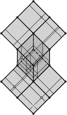
(c)

Figure 6.  (a) The cube complex ${\mathcal{D}}$ of $D$, (b) a hyperplane of $\mathcal{D}$, and (c) the box complex $\widehat{\mathcal{D}}$ and $\operatorname*{Med}_{w}({\mathcal{D}})$ (in gray) defined by 4 terminals of weight $1$.

6.2. Geometric halfspaces and hyperplanes

In the following, we fix a basepoint $v_{0}$ of $G$. For each point $x$ of $\mathcal{G}$, let $Q(x)$ be the smallest cube of $\mathcal{G}$ containing $x$ and let $v(x)$ be the gate of $v_{0}$ in $Q(x)$. For each $\Theta$-class $E_{i}$ defining a dimension of $Q(x)$, let $\epsilon_{i}(x)$ be the coordinate of $x$ along $E_{i}$ in the embedding of $Q(x)$ as a unit cube in which $v(x)$ is the origin. For a $\Theta$-class $E_{i}$ and a cube $Q$ having $E_{i}$ as a dimension, the $i$-midcube of $Q$ is the subspace of $Q$ obtained by restricting the $E_{i}$-coordinate of $Q$ to $\frac{1}{2}$. A midhyperplane $\mathfrak{h}_{i}$ of $\mathcal{G}$ is the union of all $i$-midcubes. Each $\mathfrak{h}_{i}$ cuts $\mathcal{G}$ in two components [66] and the union of each of these components with $\mathfrak{h}_{i}$ is called a geometric halfspace (see Fig. 6(b)). The carrier $\mathcal{N}_{i}$ of $E_{i}$ is the union of all cubes of $\mathcal{G}$ intersecting $\mathfrak{h}_{i}$; $\mathcal{N}_{i}$ is isomorphic to $\mathfrak{h}_{i}\times[0,1]$. For a $\Theta$-class $E_{i}$ and $0<\epsilon<1$, the hyperplane $\mathfrak{h}_{i}(\epsilon)$ is the set of all points $x\in\mathcal{N}_{i}$ such that $\epsilon_{i}(x)=\epsilon$. Let $\mathfrak{h}_{i}(0)$ and $\mathfrak{h}_{i}(1)$ be the respective geometric realizations of $\partial H_{i}^{\prime\prime}$ and $\partial H_{i}^{\prime}$. Note that $\mathfrak{h}_{i}(\epsilon)$ is obtained from $\mathfrak{h}_{i}$ by a translation. The open carrier $\mathcal{N}^{\circ}_{i}$ is $\mathcal{N}_{i}\setminus(\mathfrak{h}_{i}(0)\cup\mathfrak{h}_{i}(1))$. We denote by $\mathcal{H}^{\prime}_{i}(\epsilon)$ and $\mathcal{H}^{\prime\prime}_{i}(\epsilon)$ the geometric halfspaces of $\mathcal{G}$ defined by $\mathfrak{h}_{i}(\epsilon)$. Let $\mathcal{H}^{\prime\prime}_{i}:=\mathcal{H}^{\prime\prime}_{i}(0)$ and $\mathcal{H}^{\prime}_{i}:=\mathcal{H}^{\prime}_{i}(1)$; they are the geometric realizations of $H^{\prime}_{i}$ and $H^{\prime\prime}_{i}$. Note that $\mathcal{G}$ is the disjoint union of $\mathcal{H}^{\prime}_{i}$, $\mathcal{H}^{\prime\prime}_{i}$, and $\mathcal{N}^{\circ}_{i}$.

6.3. The majority rule for $\mathcal{G}$

Now we show how to reduce the median problem in $\mathcal{G}$ to a median problem in a median graph.

The box complex $\widehat{\mathcal{G}}$

By [74, Theorem 3.16], $(\mathcal{G},d_{1})$ is a median metric space (i.e., $|I(x,y)\cap I(y,z)\cap I(z,x)|=1$ $\forall x,y,z\in\mathcal{G}$) and the graph $G$ is isometrically embedded in $(\mathcal{G},d_{1})$. For each $p\in P$ and each coordinate $\epsilon_{i}(p)$, consider the hyperplane $\mathfrak{h}_{i}(\epsilon_{i}(p))$. All such hyperplanes subdivide $\mathcal{G}$ into a box complex $\widehat{\mathcal{G}}$ (see Fig. 6(c)). Clearly, $(\widehat{\mathcal{G}},d_{1})$ is a median space. By [74, Theorem 3.13], the 1-skeleton $\widehat{G}$ of $\widehat{\mathcal{G}}$ is a median graph and each point of $P$ corresponds to a vertex of $\widehat{G}$. The $\Theta$-classes of $\widehat{G}$ are subdivisions of the $\Theta$-classes of $G$. In $\widehat{\mathcal{G}}$, all edges of a $\Theta$-class of $\widehat{G}$ have the same length. Let $\widehat{G}_{l}$ be the graph $\widehat{G}$ in which the edges have these lengths. $\widehat{G}_{l}$ is a median space, thus $\operatorname*{Med}_{w}(\widehat{G}_{l})=\operatorname*{Med}_{w}(\widehat{G})$ by [70]. By Proposition 5.3, $\operatorname*{Med}_{w}(\widehat{G}_{l})$ is the intersection of the majoritary halfspaces of $\widehat{G}$.

Proposition 6.2.

$\operatorname*{Med}_{w}(\mathcal{G})$ is the subcomplex of $\widehat{\mathcal{G}}$ defined by $\widehat{M}:=\operatorname*{Med}_{w}(\widehat{G}_{l})$.

Proof.

Let $\widehat{E}_{1},\ldots,\widehat{E}_{\hat{q}}$ be the the $\Theta$-classes of $\widehat{G}$. For a point $x\in\mathcal{G}$, we denote by $\widehat{Q}(x)$ the smallest box of $\widehat{\mathcal{G}}$ containing $x$, and for any $\Theta$-class $\widehat{E}_{i}$ of $\widehat{Q}(x)$, let $\widehat{\epsilon}_{i}(x)$ be the coordinate of $x$ along the dimension $\widehat{E}_{i}$ in the embedding of $\widehat{Q}(x)$ as a unit cube where the origin is the gate of $v_{0}$ on $\widehat{Q}(x)$.

For a point $x\in\mathcal{G}$, let $\widehat{\mathcal{G}}(x)$ be the subdivision of the complex $\widehat{\mathcal{G}}$ by the hyperplanes passing via $x$, let $\widehat{G}(x)$ denote the 1-skeleton of $\widehat{\mathcal{G}}(x)$ and let $\widehat{G}_{l}(x)$ be the corresponding weighted graph. Again, $\widehat{G}(x)$ is a median graph and $\widehat{G}_{l}(x)$ is an isometric subgraph of $\widehat{\mathcal{G}}(x)$ that is isometric to $\mathcal{G}$ and $\widehat{\mathcal{G}}$.

We show by induction on the dimension of $\widehat{Q}(x)$ that $x\in\operatorname*{Med}_{w}(\mathcal{G})=\operatorname*{Med}_{w}(\widehat{\mathcal{G}})=\operatorname*{Med}_{w}(\widehat{\mathcal{G}}(x))$ if and only if for any vertex $v$ of $\widehat{Q}(x)$, $v\in\operatorname*{Med}_{w}(\mathcal{G})$. If $\widehat{Q}(x)=\{x\}$, then there is nothing to prove. Otherwise, pick a $\Theta$-class $\widehat{E}_{i}$ of $\widehat{G}$ such that $0<\widehat{\epsilon}_{i}(x)<1$. In $\widehat{G}(x)$, $x$ has exactly two neighbors $x^{\prime},x^{\prime\prime}$ belonging to two opposite facets of $\widehat{Q}(x)$ such that $\widehat{\epsilon}_{i}(x^{\prime\prime})=0$ and $\widehat{\epsilon}_{i}(x^{\prime})=1$. Observe that $V(\widehat{Q}(x))=V(\widehat{Q}(x^{\prime}))\cup V(\widehat{Q}(x^{\prime\prime}))$ and $x\in I_{\widehat{G}(x)}(x^{\prime},x^{\prime\prime})$. By the definition of $\widehat{G}$, there is no terminal $p\in P$ with $0<\widehat{\epsilon}_{i}(p)<1$. Consequently in $\widehat{G}(x)$, $W(x^{\prime\prime},x)\cap P=W(x,x^{\prime})\cap P$ and $W(x^{\prime},x)\cap P=W(x,x^{\prime\prime})\cap P$. Therefore in $\widehat{G}(x)$ (and in $\widehat{G}_{l}(x)$), the halfspace $W(x^{\prime\prime},x)$ is majoritary (resp. egalitarian, minoritary) if and only if $W(x^{\prime},x)$ minoritary (resp. egalitarian, majoritary).

Suppose that $x\in\operatorname*{Med}_{w}(\mathcal{G})$. If $W(x,x^{\prime\prime})$ (resp. $W(x,x^{\prime})$) is minoritary in $\widehat{G}(x)$, then by Lemma 5.2 applied to $\widehat{G}_{l}(x)$, $F_{w}(x)>F_{w}(x^{\prime\prime})$ (resp. $F_{w}(x)>F_{w}(x^{\prime})$) and $x\notin\operatorname*{Med}_{w}(\mathcal{G})$, a contradiction. Thus, necessarily $W(x^{\prime\prime},x)$ and $W(x^{\prime},x)$ are egalitarian and by Lemma 5.2 in $\widehat{G}_{l}(x)$, $F_{w}(x^{\prime})=F_{w}(x^{\prime\prime})=F_{w}(x)$. Since $\widehat{Q}(x^{\prime})$ and $\widehat{Q}(x^{\prime\prime})$ are facets of $\widehat{Q}(x)$, by induction hypothesis, all vertices in $V(\widehat{Q}(x))=V(\widehat{Q}(x^{\prime}))\cup V(\widehat{Q}(x^{\prime\prime}))$ belong to $\operatorname*{Med}_{w}(\mathcal{G})$. Conversely, suppose that $V(\widehat{Q}(x))=V(\widehat{Q}(x^{\prime}))\cup V(\widehat{Q}(x^{\prime\prime}))\subseteq\operatorname*{Med}_{w}(\mathcal{G})$. Then by induction hypothesis, $x^{\prime},x^{\prime\prime}\in\operatorname*{Med}_{w}(\mathcal{G})$. Since $\operatorname*{Med}_{w}(\widehat{G}_{l}(x))=\operatorname*{Med}_{w}(\widehat{G}(x))$ is convex and $x\in I_{\widehat{G}(x)}(x,x^{\prime})$, we have $F_{w}(x)=F_{w}(x^{\prime})=F_{w}(x^{\prime\prime})$ and consequently, $x\in\operatorname*{Med}_{w}(\mathcal{G})$. ∎

The $E_{i}$-median problems

We adapt now Proposition 5.3 to the continuous setting. In our algorithm and next results we will not explicitly construct the box complex $\widehat{\mathcal{G}}$ and its 1-skeleton $\widehat{G}$ (because they are too large), but we will only use them in proofs. For a $\Theta$-class of $G$, the $E_{i}$-median is the median of the multiset of points of the segment $[0,1]$ weighted as follows: the weight $w_{i}(0)$ of $0$ is $w(\mathcal{H}^{\prime\prime}_{i})$, the weight $w_{i}(1)$ of 1 is $w(\mathcal{H}^{\prime}_{i})$, and for each $p\in P\cap\mathcal{N}_{i}^{\circ}$, there is a point $\epsilon_{i}(p)$ of $[0,1]$ of weight $w_{i}(\epsilon_{i}(p))=w(p)$. It is well-known that this median is a segment $[\varrho^{\prime\prime}_{i},\varrho^{\prime}_{i}]$ defined by two consecutive points $\varrho^{\prime\prime}_{i}\leq\varrho^{\prime}_{i}$ of $[0,1]$ with positive weights, and for any $p\in P$, $\epsilon_{i}(p)\leq\varrho_{i}^{\prime\prime}$ or $\epsilon_{i}(p)\geq\varrho_{i}^{\prime}$. Majoritary, minoritary, and egalitarian geometric halfspaces of $\mathcal{G}$ are defined in the same way as the halfspaces of $G$.

Proposition 6.3.

Let $E_{i}$ be a $\Theta$-class of $G$. Then the following holds:

1. $\operatorname*{Med}_{w}(\mathcal{G})\subseteq\mathcal{H}^{\prime\prime}_{i}$ (resp. $\operatorname*{Med}_{w}(\mathcal{G})\subseteq\mathcal{H}^{\prime}_{i}$) if and only if $\mathcal{H}^{\prime\prime}_{i}$ is majoritary (resp. $\mathcal{H}^{\prime}_{i}$ is majoritary), i.e., $\rho_{i}^{\prime\prime}=\rho_{i}^{\prime}=0$ (resp. $\rho_{i}^{\prime\prime}=\rho_{i}^{\prime}=1$);

2. $\operatorname*{Med}_{w}(\mathcal{G})\subseteq\mathcal{H}^{\prime\prime}_{i}\cup\mathcal{N}^{\circ}_{i}$ (resp. $\operatorname*{Med}_{w}(\mathcal{G})\subseteq\mathcal{H}^{\prime}_{i}\cup\mathcal{N}^{\circ}_{i}$) and $\operatorname*{Med}_{w}(\mathcal{G})$ intersects each of the sets $\mathcal{H}^{\prime\prime}_{i}$ (resp. $\mathcal{H}^{\prime}_{i}$) and $\mathcal{N}^{\circ}_{i}$ if and only if $\mathcal{H}^{\prime\prime}_{i}$ (resp. $\mathcal{H}^{\prime}_{i}$) is egalitarian and $\mathcal{H}^{\prime}_{i}$ (resp. $\mathcal{H}^{\prime\prime}_{i}$) is minoritary, i.e., $0=\rho_{i}^{\prime\prime}<\rho_{i}^{\prime}<1$ (resp. $0<\rho_{i}^{\prime\prime}<\rho_{i}^{\prime}=1$);

3. $\operatorname*{Med}_{w}(\mathcal{G})\subseteq\mathcal{N}^{\circ}_{i}$ if and only if $\mathcal{H}^{\prime}_{i}$ and $\mathcal{H}^{\prime\prime}_{i}$ are minoritary, i.e., $0<\rho_{i}^{\prime\prime}\leq\rho_{i}^{\prime}<1$;

4. $\operatorname*{Med}_{w}(\mathcal{G})$ intersects the three sets $\mathcal{H}_{i},\mathcal{H}^{\prime\prime}_{i},$ and $\mathcal{N}^{\circ}_{i}$ if and only if $\mathcal{H}^{\prime}_{i}$ and $\mathcal{H}^{\prime\prime}_{i}$ are egalitarian, i.e., $0=\rho_{i}^{\prime\prime}\leq\rho_{i}^{\prime}=1$ (and thus $w(\mathcal{N}^{\circ}_{i})=0$).

Proof.

Let $0<\epsilon_{1}<\cdots<\epsilon_{k}<1$ denote the possible values of coordinates of points of $P$ with respect to the $\Theta$-class $E_{i}$. They define parallel hyperplanes $\mathfrak{h}_{i}(0),\mathfrak{h}_{i}(\epsilon_{1}),\ldots,\mathfrak{h}_{i}(\epsilon_{k}),\mathfrak{h}_{i}(1)$. The pieces of the edges of $E_{i}$ bounded by two such consecutive hyperplanes define a $\Theta$-class of $\widehat{G}$ and all such $\Theta$-classes are laminar. In fact, we have the following chains of inclusions between the geometric halfspaces of $\mathcal{G}$ (or $\widehat{\mathcal{G}}$) defined by those $\Theta$-classes: $\mathcal{H}^{\prime\prime}_{i}=\mathcal{H}_{i}^{\prime\prime}(0)\subset\mathcal{H}^{\prime\prime}_{i}(\epsilon_{1})\subset\cdots\subset\mathcal{H}^{\prime\prime}_{i}(\epsilon_{k})$ and $\mathcal{H}^{\prime}_{i}=\mathcal{H}^{\prime}_{i}(1)\subset\mathcal{H}^{\prime}_{i}(\epsilon_{k})\subset\cdots\subset\mathcal{H}^{\prime}_{i}(\epsilon_{1})$. Similar inclusions hold between corresponding halfspaces of the graph $\widehat{G}$. Notice also that, by the definition of $\widehat{G}$ and $\widehat{\mathcal{G}}$, the geometric halfspaces and the corresponding graphic halfspaces, have the same weight. Therefore, to deduce the different cases of the proposition, it suffices to apply the majority rule (Proposition 5.3 and Corollary 5.7) to the halfspaces of $\widehat{G}$ occurring in the two chains of inclusions and use the fact that $\widehat{M}$ is the $1$-skeleton of $\operatorname*{Med}_{w}(\mathcal{G})=\operatorname*{Med}_{w}(\widehat{\mathcal{G}})$ in $\widehat{\mathcal{G}}$ from Proposition 6.2. ∎

6.4. The algorithm

Data: A median graph $G=(V,E)$, a set of terminals $P$, a weight function $w:P\rightarrow\mathbb{R}^{+}$, the $\Theta$-classes $\Theta=(E_{1},\ldots,E_{q})$ of $G$ ordered by increasing distance to the basepoint $v_{0}$.

Result: The graph $\widehat{M}$ and the coordinates of each vertex $\widehat{m}\in\widehat{M}$ in $\mathcal{G}$

begin

       Modify the root $v(p)$ of each point $p\in P$ such that $v(p)$ is the gate of $v_{0}$ on $Q(p)$

       Compute $w(P_{i})$ for all $\Theta$-classes $E_{i}$ by traversing $P$

       Compute $w_{*}(v)=w(P_{v})$ for all $v\in V$ by traversing $P$

       Apply ComputeWeightsOfHalfspaces $(G,w_{*},\Theta)$ to compute the weights $w_{*}(H_{i}^{\prime})$ and $w_{*}(H_{i}^{\prime\prime})$ for each $\Theta$-class $E_{i}$

       Set $w(\mathcal{H}_{i}^{\prime})\leftarrow w_{*}(H_{i}^{\prime})$ and $w(\mathcal{H}_{i}^{\prime\prime})\leftarrow w_{*}(H_{i}^{\prime\prime})-w(P_{i})$ for each $\Theta$-class $E_{i}$

       Compute the $E_{i}$-median instance for all $\Theta$-classes $E_{i}$ by traversing $P$

       Compute the $E_{i}$-median $[\varrho_{i}^{\prime\prime},\varrho_{i}^{\prime}]$ for each $\Theta$-class $E_{i}$

       Orient the edges of $G$ and compute the set of half-edges around each vertex $v\in V$

       Compute the set $S(\overrightarrow{G})$ of sinks of $\overrightarrow{G}$ by traversing the edges of $G$

       $V(\widehat{M})\leftarrow\left\{g(v):v\in S(\overrightarrow{G})\right\}$

       $E(\widehat{M})n\leftarrow\left\{g(u)g(v):uv\in E\text{ and }u,v\in S(\overrightarrow{G})\right\}$

       return $\left(V(\widehat{M}),E(\widehat{M})\right)$

      

Algorithm 4 ComputeMedianCubeComplex($G,P,w,\Theta$)

Preprocessing the input

We first compute the $\Theta$-classes $E_{1},E_{2},\ldots,E_{q}$ of $G$ ordered by increasing distance from $v_{0}$ to $H^{\prime}_{i}$. Using this, we first modify the input of the median problem in linear time $O(m+\delta)$ in such a way that for each terminal $p\in P$, $v(p)$ is the gate of $v_{0}$ in $Q(p)$. Once the $\Theta$-classes have been computed, we can assume that each terminal $p$ is described by its root $v(p)$ as well as a list of coordinates $\Delta(p)$, one coordinate $0<\epsilon_{i}(p)<1$ for each $\Theta$-class $E_{i}$ of $Q(p)$ such that $\epsilon_{i}(p)$ is the coordinate of $x$ along $E_{i}$ in the embedding of $Q(p)$ as a unit cube in which $v(p)$ is the origin. To update $v(p)$ and $\Delta(p)$, we use a (non-initialized) matrix $B$ whose rows and columns are indexed respectively by the vertices and the $\Theta$-classes of $G$ and such that if a vertex $v$ has a neighbor $v^{\prime}$ such that $vv^{\prime}$ belongs to the $\Theta$-class $E_{i}$, then $B[v,E_{i}]=v^{\prime}$ (and $B[v,E_{i}]$ is undefined if $v$ does not have such a neighbor $v^{\prime}$). One can construct $B$ in time $O(m)$ by traversing all edges of $G$ once the $\Theta$-classes have been computed. With the matrix $B$ at hand, for each terminal $p\in P$, we consider the coordinates of $p$ in order and for each coordinate $\epsilon_{i}(p)$ of $p$, if $v^{\prime}=B[v(p),E_{i}]$ is closer to $v_{0}$ than $v(p)$, we replace $v(p)$ by $v^{\prime}$ and $\epsilon_{i}(p)$ by $1-\epsilon_{i}(p)$. Observe that each time we modify $v(p)$, $v(p)$ is still a vertex of $Q(p)$ and thus $B[v(p),E_{j}]$ is still defined for any coordinate $\epsilon_{j}\in\Delta(p)$. Note that $v(p)$ can move to distance up to $|\Delta(p)|$ from its original position during the process. Once the matrix $B$ has been computed, the modification of the roots of all the points $p\in P$ can be performed in time $O(\sum_{p\in P}\Delta(p))=O(\delta)$.

In this way, the local coordinates of the terminals of $P$ coincide with the coordinates $\epsilon_{i}(p)$ defined in Section 6.2. For each $\Theta$-class $E_{i}$, let $P_{i}=P\cap\mathcal{N}^{\circ}_{i}=\{p\in P:0<\epsilon_{i}(p)<1\}$, and for each point $v\in V(G)$, let $P_{v}=\{p\in P:v(p)=v\}$. By traversing the points of $P$, we can compute all sets $P_{i}$, $1\leq i\leq q$ and $P_{v}$, $v\in V$ and the weights of these sets in time $O(\delta)$.

Computing the $E_{i}$-medians

We first compute the weights $w_{i}(0)=w(\mathcal{H}_{i}^{\prime\prime})$ and $w_{i}(1)=w(\mathcal{H}_{i}^{\prime})$ of the geometric halfspaces $\mathcal{H}_{i}^{\prime\prime},\mathcal{H}_{i}^{\prime}$ of $G$. For each vertex $v$ of $G$, let ${w}_{*}(v)=w(P_{v})$. Note that ${w}_{*}(V)=w(P)$. Since $v_{0}\in H_{i}^{\prime\prime}$, ${w}_{*}(H_{i}^{\prime})=w(\mathcal{H}_{i}^{\prime})$ and ${w}_{*}(H_{i}^{\prime\prime})=w(\mathcal{H}_{i}^{\prime\prime})+w(\mathcal{N}_{i}^{o})$ for each $\Theta$-class $E_{i}$. We apply the algorithm of Section 5.2 to $G$ with the weight function ${w}_{*}$ to compute the weights ${w}_{*}(H_{i}^{\prime})$ and ${w}_{*}(H_{i}^{\prime\prime})$ of all halfspaces of $G$. Since $w(\mathcal{N}_{i}^{o})=w(P_{i})$ is known, we can compute $w(\mathcal{H}_{i}^{\prime})={w}_{*}(H_{i}^{\prime})$ and $w(\mathcal{H}_{i}^{\prime\prime})={w}_{*}(H_{i}^{\prime\prime})-w(P_{i})$. This allows us to complete the definition of each $E_{i}$-median problem which altogether can be solved linearly in the size of the input [30, Problem 9.2], i.e., in time $O(\Sigma_{i=1}^{q}(|P_{i}|+2))=O(\delta+m)$.

Computing $\widehat{M}$

To compute the 1-skeleton $\widehat{M}$ of $\operatorname*{Med}_{w}(\mathcal{G})$ in $\widehat{G}$, we orient the edges of $E_{i}$ according to the weights of $\mathcal{H}^{\prime}_{i}$ and $\mathcal{H}^{\prime\prime}_{i}$: $v^{\prime}v^{\prime\prime}\in E_{i}$ with $v^{\prime}\in\mathcal{H}^{\prime}_{i}$ and $v^{\prime\prime}\in\mathcal{H}^{\prime\prime}_{i}$ is directed from $v^{\prime\prime}$ to $v^{\prime}$ if $\varrho^{\prime}_{i}=\varrho^{\prime\prime}_{i}=1$ ($\mathcal{H}^{\prime}_{i}$ is majoritary) and from $v^{\prime}$ to $v^{\prime\prime}$ if $\varrho^{\prime}_{i}=\varrho^{\prime\prime}_{i}=0$ ($\mathcal{H}^{\prime\prime}_{i}$ is majoritary), otherwise the edges of $E_{i}$ are not oriented. Denote this partially directed graph by $\overrightarrow{G}$ and let $S(\overrightarrow{G})$ be the set of sinks of $\overrightarrow{G}$. A non-directed edge $v^{\prime}v^{\prime\prime}\in E_{i}$ defines a half-edge with origin $v^{\prime\prime}$ if $\varrho^{\prime\prime}_{i}>0$ and a half-edge with origin $v^{\prime}$ if $\varrho^{\prime}_{i}<1$ (an edge $v^{\prime}v^{\prime\prime}$ such that $0<\varrho^{\prime\prime}_{i}\leq\varrho^{\prime}_{i}<1$ defines two half-edges).

Proposition 6.4.

For any vertex $v$ of $\overrightarrow{G}$, all half-edges with origin $v$ define a cube $Q_{v}$ of $\mathcal{G}$.

Proof.

For any vertex $v$ and two $\Theta$-classes $E_{i},E_{j}$ defining half-edges with origin $v$, let $v_{i}$ and $v_{j}$ be the respective neighbors of $v$ in $\widehat{G}$ along the directions $E_{i}$ and $E_{j}$. By Proposition 6.3, $vv_{i}$ and $vv_{j}$ point to two majoritary halfspaces of $\widehat{G}$ (and $\mathcal{G}$). Since those two halfspaces cannot be disjoint, $E_{i}$ and $E_{j}$ are crossing. The proposition then follows from Lemma 3.7. ∎

For any cube $Q$ of $\mathcal{G}$, let $B(Q)\subseteq Q$ be the subcomplex of $\widehat{\mathcal{G}}$ that is the Cartesian product of the $E_{i}$-medians $[\varrho^{\prime\prime}_{i},\varrho^{\prime}_{i}]$ over all $\Theta$-classes $E_{i}$ wich define dimensions of $Q$. By the definition of the $E_{i}$-medians, $B(Q)$ is a single box of $\widehat{\mathcal{G}}$ and its vertices belong to $\widehat{G}$.

Proposition 6.5.

For any cube $Q$ of $\mathcal{G}$, if $Q\cap\operatorname*{Med}_{w}(\mathcal{G})\neq\emptyset$, then $B(Q)=\operatorname*{Med}_{w}(\mathcal{G})\cap Q$.

Proof.

If a vertex $x$ of $B(Q)$ is not a median of $\widehat{G}$, by Proposition 5.3, $x$ is not a local median of $\widehat{G}$. Thus $F_{w}(x)>F_{w}(y)$ for an edge $xy$ of $\widehat{G}$. Suppose that $xy$ is parallel to the edges of $E_{i}$ of $G$. Then $\epsilon_{i}(x)$ coincides with $\varrho^{\prime\prime}_{i}$ or $\varrho^{\prime}_{i}$. Since $F_{w}(x)>F_{w}(y)$, the halfspace $W(y,x)$ of $\widehat{G}$ is majoritary, contrary to the assumption that $\epsilon_{i}(x)$ is an $E_{i}$-median point. Thus all vertices of $B(Q)$ belong to $\widehat{M}$ and by Proposition 6.2, $B(Q)\subseteq\operatorname*{Med}_{w}(\mathcal{G})$. It remains to show that any point of $Q\setminus B(Q)$ is not median. Otherwise, by Proposition 6.2 and since $\widehat{M}$ is convex, there exists a vertex $y\notin B(Q)$ of $(\widehat{M}\cap Q)\setminus B(Q)$ adjacent to a vertex $x$ of $B(Q)$. Let $xy$ be parallel to $E_{i}$. Then $\epsilon_{i}(x)$ coincides with $\varrho^{\prime\prime}_{i}$ or $\varrho^{\prime}_{i}$ and $\epsilon_{i}(y)$ does not belong to the $E_{i}$-median $[\varrho^{\prime\prime}_{i},\varrho^{\prime}_{i}]$. Hence the halfspace $W(y,x)$ of $\widehat{G}$ is minoritary, contrary to $F_{w}(y)=F_{w}(x)$. ∎

For a sink $v$ of $\overrightarrow{G}$, let $g(v)$ be the point of $Q_{v}$ such that for each $\Theta$-class $E_{i}$ of $Q_{v}$, $\epsilon_{i}(g(v))=\varrho^{\prime}$ if $v\in\mathcal{H}_{i}^{\prime}$ and $\epsilon_{i}(g(v))=\varrho^{\prime\prime}$ if $v\in\mathcal{H}_{i}^{\prime\prime}$. Note that $g(v)$ is the gate of $v$ in $B(Q_{v})$ and $g(v)$ is a vertex of $\widehat{M}$. Conversely, let $x\in\widehat{M}$ and consider the cube $Q(x)$. Since $B(Q(x))$ is a cell of $\widehat{\mathcal{G}}$, for each $\Theta$-class $E_{i}$ of $Q(x)$, we have $\epsilon_{i}(x)\in\{\varrho^{\prime}_{i},\varrho_{i}^{\prime\prime}\}$. Let $f(x)$ be the vertex of $Q(x)$ such that $f(x)\in\mathcal{H}_{i}^{\prime\prime}$ if $\epsilon_{i}(x)=\varrho^{\prime\prime}_{i}$ and $f(x)\in\mathcal{H}_{i}^{\prime}$ otherwise.

Proposition 6.6.

For any $v\in S(\overrightarrow{G})$, $g(v)$ is the gate of $v$ in $\widehat{M}$ and $\operatorname*{Med}_{w}(\mathcal{G})$. For any $x\in\widehat{M}$, $x=g(f(x))$ is the gate of $f(x)$ in $\widehat{M}$ and $\operatorname*{Med}_{w}(\mathcal{G})$.

Furthermore, for any edge $uv$ of $G$ with $u,v\in S(\overrightarrow{G})$, either $g(u)=g(v)$ or $g(u)g(v)$ is an edge of $\widehat{M}$. Conversely, for any edge $xy$ of $\widehat{M}$, $f(x)f(y)$ is an edge of $G$.

Proof.

By Proposition 6.3 applied to $\mathcal{G}$, Proposition 5.3 applied to $\widehat{G}$, and the definition of sinks of $\overrightarrow{\widehat{G}}$, $g(v)$ is a sink of $\overrightarrow{\widehat{G}}$, thus $g(v)$ is a median of $\widehat{G}$ and $\mathcal{G}$. Since $B(Q_{v})=\operatorname*{Med}_{w}(\mathcal{G})\cap Q_{v}$ is gated and non-empty, the gate of $v$ in $\operatorname*{Med}_{w}(\mathcal{G})$ belongs to $B(Q_{v})$ and thus the gate of $v$ in $\operatorname*{Med}_{w}(\mathcal{G})$ is the gate of $v$ on $B(Q_{v})$. Conversely, $\epsilon_{i}(x)\notin\{0,1\}$ for any $E_{i}$ defining a dimension of $Q(x)$, thus there is an $E_{i}$-half-edge with origin $f(x)$. Pick now any $E_{j}$-edge incident to $v$ such that $E_{j}$ does not define a dimension of $Q(x)$. Without loss of generality, assume that $f(x)\in\mathcal{H}_{j}^{\prime}$. Then $x\in\mathcal{H}_{j}^{\prime}$, yielding $w(\mathcal{H}_{j}^{\prime})\geq\frac{1}{2}w(P)$. By Proposition 6.3, $\varrho_{j}^{\prime}=1$ and thus $f(x)$ is not the origin of an $E_{j}$-edge or $E_{j}$-half-edge. Consequently, $Q_{f(x)}=Q(x)$ by Proposition 6.4 and by the definition of $f(x)$ and $g(f(x))$, we have $x=g(f(x))$.

Let $v^{\prime}v^{\prime\prime}$ be an $E_{i}$-edge between two sinks of $\overrightarrow{G}$ with $v^{\prime}\in\mathcal{H}_{i}^{\prime}$ and $v^{\prime\prime}\in\mathcal{H}^{\prime\prime}_{i}$. Let $x^{\prime}=g(v^{\prime})$ and $x^{\prime\prime}=g(v^{\prime\prime})$ and assume that $x^{\prime}\neq x^{\prime\prime}$. Let $u^{\prime},u^{\prime\prime}$ be the points of $v^{\prime}v^{\prime\prime}$ such that $\epsilon_{i}(u^{\prime})=\varrho_{i}^{\prime}$ and $\epsilon_{i}(u^{\prime\prime})=\varrho_{i}^{\prime\prime}$. Note that $u^{\prime}$ and $u^{\prime\prime}$ are adjacent vertices of $\widehat{G}$ and that $u^{\prime}\in I_{\widehat{G}}(v^{\prime},x^{\prime})$ and $u^{\prime\prime}\in I_{\widehat{G}}(v^{\prime\prime},x^{\prime\prime})$. In $\widehat{G}$, $x^{\prime\prime}$ is the gate of $u^{\prime\prime}$ (and $x^{\prime}$ is the gate of $u^{\prime}$) in $\widehat{M}$. Since $d_{\widehat{G}}(u^{\prime},x^{\prime})+d_{\widehat{G}}(x^{\prime},x^{\prime\prime})=d_{\widehat{G}}(u^{\prime},x^{\prime\prime})\leq d_{\widehat{G}}(u^{\prime\prime},x^{\prime\prime})+1$ and $d_{\widehat{G}}(u^{\prime\prime},x^{\prime\prime})+d_{\widehat{G}}(x^{\prime},x^{\prime\prime})=d_{\widehat{G}}(u^{\prime\prime},x^{\prime})\leq d_{\widehat{G}}(u^{\prime},x^{\prime})+1$, we obtain that $d_{\widehat{G}}(x^{\prime},x^{\prime\prime})\leq 1$.

Any edge $x^{\prime}x^{\prime\prime}$ of $\widehat{M}$ is parallel to a $\Theta$-class $E_{i}$ of $G$. For any $\Theta$-class $E_{j}$ of $Q(x^{\prime})$ (resp. $Q(x^{\prime\prime})$) with $j\neq i$, $E_{j}$ is a $\Theta$-class of $Q(x^{\prime\prime})$ (resp. $Q(x^{\prime})$) and $\epsilon_{j}(x^{\prime})=\epsilon_{j}(x^{\prime\prime})$. By their definition, $f(x^{\prime})$ and $f(x^{\prime\prime})$ can be separated only by $E_{i}$, i.e., $d_{G}(f(x^{\prime}),f(x^{\prime\prime}))\leq 1$. Since $f$ is an injection from $V(\widehat{M})$ to $S(\overrightarrow{G})$, necessarily $f(x^{\prime})$ and $f(x^{\prime\prime})$ are adjacent. ∎

The algorithm computes the set $S(\overrightarrow{G})$ of all sinks of $\overrightarrow{G}$ and for each sink $v\in S(\overrightarrow{G})$, it computes the gate of $g(v)$ of $v$ in $\widehat{M}$ and the local coordinates of $g(v)$ in $\mathcal{G}$. The algorithm returns $\left\{g(v):v\in S(\overrightarrow{G})\right\}$ as $V(\widehat{M})$ and $\left\{g(u)g(v):uv\in E\text{ and }u,v\in S(\overrightarrow{G})\right\}$ as $E(\widehat{M})$. Proposition 6.6 implies that $V(\widehat{M})$ and $E(\widehat{M})$ are correctly computed and that $\widehat{M}$ contains at most $n$ vertices and $m$ edges. Moreover each vertex $x$ of $\widehat{M}$ is the gate $g(f(x))$ of the vertex $f(x)$ of $Q(x)$ that has dimension at most $\deg(f(x))$. Hence the size of the description of the vertices of $\widehat{M}$ is at most $O(m)$. This finishes the proof of Theorem 6.1.

6.5. Wiener index in $\mathcal{G}$

We describe a linear time algorithm to compute the Wiener index of a set of terminals in the $\ell_{1}$-cube complex $\mathcal{G}$ of a median graph $G$. By analogy with graphs, the Wiener index in $\mathcal{G}$ is the sum of the weighted distances between all pairs of terminals.

Proposition 6.7.

Let $G$ be a median graph with $m$ edges and let $P$ be a finite set of terminals of $\mathcal{G}$ described by an input of size $\delta$. The Wiener index of $P$ in $\mathcal{G}$ can be computed in $O(m+\delta)$ time.

Proof.

The proof is similar to the proof of Proposition 5.11. Let $0<\epsilon_{1}<\cdots<\epsilon_{k}<1$ denote the $E_{i}$-coordinates of the points in $P$ and let $\epsilon_{0}=0$ and $\epsilon_{k+1}=1$. Just like in the proof of Proposition 6.3, we have the following chains of inclusions between the halfspaces defined by the hyperplanes $\mathfrak{h}_{i}(\epsilon_{0}),\mathfrak{h}_{i}(\epsilon_{1}),\ldots,\mathfrak{h}_{i}(\epsilon_{k}),\mathfrak{h}_{i}(\epsilon_{k+1})$:

$$\mathcal{H}^{\prime\prime}_{i}=\mathcal{H}_{i}^{\prime\prime}(\epsilon_{0})\subset\mathcal{H}^{\prime\prime}_{i}(\epsilon_{1})\subset\cdots\subset\mathcal{H}^{\prime\prime}_{i}(\epsilon_{k})$$

and

$$\mathcal{H}^{\prime}_{i}=\mathcal{H}^{\prime}_{i}(\epsilon_{k+1})\subset\mathcal{H}^{\prime}_{i}(\epsilon_{k})\subset\cdots\subset\mathcal{H}^{\prime}_{i}(\epsilon_{1}).$$

Then, similarly to Lemma 5.12, we get the following result:

Lemma 6.8.

$W_{w}(\mathcal{G})=\sum_{i=1}^{q}\sum_{j=0}^{k}w(\mathcal{H}^{\prime\prime}_{i}(\epsilon_{j}))\cdot w(\mathcal{H}^{\prime}_{i}(\epsilon_{j+1}))\cdot(\epsilon_{j+1}-\epsilon_{j})$.

Once the $O(\delta)$ hyperplanes are ordered, we can compute the weights of the halfspaces in $O(m+\delta)$ time and compute the Wiener index of $P$ in $\mathcal{G}$ in $O(m+\delta)$ time. ∎

7. The median problem in event structures

In this section, we consider the median problem in which the median graph is implicitly defined as the domain of configurations of an event structure. We show that the problem can be solved efficiently in the size of the input. However, if the input consists solely of the event structure and the goal is to compute the median of all configurations of the domain, then this algorithmic problem is $\#$P-hard. To prove this we provide a direct (polynomial size) correspondence between event structures and 2-SAT formulas and use $\#$P-hardness of a similar median problem for 2-SAT established in [36].

7.1. Definitions and bijections

We start with the definition of event structures and 2-SAT formulas and their bijections with median graphs.

7.1.1. Event structures

Event structures, introduced by Nielsen, Plotkin, and Winskel [58, 77], are a widely recognized abstract model of concurrent computation. An event structure is a triple ${\mathcal{E}}=(E,\leq,\#)$, where

• $E$ is a set of events,

• $\leq\subseteq E\times E$ is a partial order of causal dependency,

• $\#\subseteq E\times E$ is a binary, irreflexive, symmetric relation of conflict,

• $\downarrow\!e:=\{e^{\prime}\in E:e^{\prime}\leq e\}$ is finite for any $e\in E$,

• $e\#e^{\prime}$ and $e^{\prime}\leq e^{\prime\prime}$ imply $e\#e^{\prime\prime}$.

Two events $e^{\prime},e^{\prime\prime}$ are concurrent (notation $e^{\prime}\|e^{\prime\prime}$) if they are order-incomparable and they are not in conflict. A configuration of an event structure ${\mathcal{E}}$ is any finite subset $c\subset E$ of events which is conflict-free ($e,e^{\prime}\in c$ implies that $e,e^{\prime}$ are not in conflict) and downward-closed ($e\in c$ and $e^{\prime}\leq e$ implies that $e^{\prime}\in c$). Notice that $\varnothing$ is always a configuration and that $\downarrow\!e$ and $\downarrow\!e\setminus\{e\}$ are configurations for any $e\in E$. The domain of $\mathcal{E}$ is the set $\mathcal{D}({\mathcal{E}})$ of all configurations of ${\mathcal{E}}$ ordered by inclusion; $(c^{\prime},c)$ is a (directed) edge of the Hasse diagram of the poset $({\mathcal{D}}({\mathcal{E}}),\subseteq)$ if and only if $c=c^{\prime}\cup\{e\}$ for an event $e\in E\setminus c$. The domain $\mathcal{D}(\mathcal{E})$ can be endowed with the Hamming distance $d(c,c^{\prime})=|c\Delta c^{\prime}|$ between any configurations $c$ and $c^{\prime}$. From the following result, the Hamming distance coincides with the graph-distance. Barthélemy and Constantin [13] established the following bijection between event structures and pointed median graphs:

Theorem 7.1 (​​[13]).

The (undirected) Hasse diagram of the domain $(\mathcal{D}(\mathcal{E}),\subseteq)$ of an event structure $\mathcal{E}=(E,\leq,\#)$ is median. Conversely, for any median graph $G$ and any basepoint $v$ of $G$, the pointed median graph $G_{v}$ is the Hasse diagram of the domain of an event structure $\mathcal{E}_{v}$.

We briefly recall the construction of the event structure $\mathcal{E}_{v}$. Consider a median graph $G$ and an arbitrary basepoint $v$. The events of the event structure $\mathcal{E}_{v}$ are the hyperplanes of the cube complex $\mathcal{G}$ (or the $\Theta$-classes of $G$). Two hyperplanes $H$ and $H^{\prime}$ define concurrent events if and only if they cross (i.e., there exist a square with two opposite edges in one $\Theta$-class and other two opposite edges in the second $\Theta$-class). The hyperplanes $H$ and $H^{\prime}$ are in relation $H\leq H^{\prime}$ if and only if $H=H^{\prime}$ or $H$ separates $H^{\prime}$ from $v$. Finally, the events defined by $H$ and $H^{\prime}$ are in conflict if and only if $H$ and $H^{\prime}$ do not cross and neither separates the other from $v$.

Example 7.2.

The pointed median graph $G$ described in Fig. 7 is the domain of the event structure $\mathcal{E}=(E,\leq,\#)$. The seven events $e_{1},\ldots,e_{7}$ of $E$ correspond to the seven $\Theta$-classes of $G$. The causal dependency is defined by $e_{1}\leq e_{3},e_{5},e_{6},e_{7}$; $e_{2}\leq e_{4},e_{5},e_{6},e_{7}$; $e_{3},e_{4},e_{5}\leq e_{6},e_{7}$. The events $e_{6}$ and $e_{7}$ are in conflict and all remaining pairs of events are concurrent.

Figure 7. The domain of the event structure from Example 7.2.

Consequently, event structures encode median graphs and this representation is much more compact than the standard one using vertices and edges. For example, the hypercube of dimension $d$ is the domain of the event structure with $d$ events that are pairwise concurrent.

7.1.2. The median problem in event structures

Let ${\mathcal{E}}=(E,\leq,\#)$ be a finite event structure. The input is a set $C=\{c_{1},\ldots,c_{k}\}$ of configurations of $\mathcal{E}$ and their weights $w_{1},\ldots,w_{k}$, where each $c_{i}$ is given by the list of events belonging to $c_{i}$. The goal of the median problem in the event structure $\mathcal{E}$ is to compute a configuration $c$ minimizing the function $F_{w}(c)=\sum_{i=1}^{k}w_{i}d(c,c_{i})$, where $d(c,c^{\prime})$ is the Hamming distance between $c$ and $c^{\prime}$. Consider also a special case of this median problem, in which $C$ is the set of all configurations of $\mathcal{E}$ and the input is the event structure $\mathcal{E}$, i.e., the graphs $(E,\leq)$ and $(E,\#)$. We call this problem the compact median problem.

7.1.3. 2-SAT formulas

A 2-SAT formula on variables $x_{1},\ldots,x_{n}$ is a formula $\varphi$ in conjunctive normal form with two literals per clause, i.e., a set of clauses of the form $(u\vee v)$, where each of the two literals $u,v$ is either a positive literal $x_{i}$ or a negative literal $\neg x_{i}$. A solution for $\varphi$ is an assignment $S$ of variables to 0 or 1 that satisfies all clauses. The solution set ${\mathcal{S}}(\varphi)$ of $\varphi$ is the set of all solutions of $\varphi$. We consider each solution set as a subset of vertices of the $n$-dimensional hypercube $Q_{n}$. A subset $Y$ of vertices of the hypercube $Q_{n}$ (viewed as a median graph) is called median-stable if the median of each triplet $x,y,z\in Y$ also belongs to $Y$.

Proposition 7.3 (​​[69, 56]).

Median-stable sets are exactly the solution sets of 2-SAT formulas.

A variable of a 2-SAT formula $\varphi$ is trivial if it has the same value in each solution. Two nontrivial variables $x_{i}$ and $x_{j}$ in $\varphi$ are equivalent if either $x_{i}=x_{j}$ in all solutions or $x_{i}=\neg x_{j}$ in all solutions. Here is a characterization of 2-SAT formulas corresponding to median graphs:

Proposition 7.4 (​​[36, Corollary 3.34]).

The solution set ${\mathcal{S}}(\varphi)$ of a 2-SAT formula $\varphi$ induces a median graph if and only if $\varphi$ has no equivalent variables.

7.2. A direct correspondence between event structures and 2-SAT formulas

We provide a canonical correspondence between event structures and 2-SAT formulas (which may be useful also for other purposes).

By Theorem 7.1 and Propositions 7.3,7.4 there is a bijection between the domains of event structures and pointed median graphs and a bijection between (unpointed) median graphs and 2-SAT formulas not containing equivalent variables. Since $\varnothing$ and $\downarrow\!e,e\in E$ are configurations, their characteristic vectors must be solutions of the associated 2-SAT formula. This can be ensured by requiring that the 2-SAT formula does not contain clauses of the form $(x_{i}\vee x_{j})$.

Let $\mathcal{E}=(E,\leq,\#)$ be an event structure with $E=\{e_{1},\ldots,e_{n}\}$. We associate to $\mathcal{E}$ a 2-SAT formula $\varphi_{\mathcal{E}}$ on $n$ variables $x_{1},\ldots,x_{n}$. For each pair of events such that $e_{i}\leq e_{j}$ we define the clause $(x_{i}\vee\neg x_{j})$ and for each pair of events such that $e_{i}\#e_{j}$ we assign the clause $(\neg x_{i}\vee\neg x_{j})$. Next for each subset $c$ of $E$ we denote by $S_{c}$ its characteristic vector.

Proposition 7.5.

${\mathcal{S}}(\varphi_{\mathcal{E}})$ coincides with $\mathcal{D}(\mathcal{E})$.

Proof.

Let $c\subseteq E$ and $c\notin\mathcal{D}(\mathcal{E})$, i.e., $c$ is either not downward-closed or not conflict-free. In the first case, there exist two events $e_{i}$ and $e_{j}$ such that $e_{i}\leq e_{j}$ and $e_{j}\in c,e_{i}\notin c$. This implies that $\varphi_{\mathcal{E}}$ contains the clause $(\neg x_{j}\vee x_{i})$. Since $S_{c}(x_{j})=1$ and $S_{c}(x_{i})=0$, $S_{c}$ is not a solution of $\varphi_{\mathcal{E}}$. In the second case, there exist two events $e_{i},e_{j}\in c$ such that $e_{i}\#e_{j}$. This implies that $\varphi_{\mathcal{E}}$ contains the clause $(\neg x_{i}\vee\neg x_{j})$. Since $S_{c}(x_{i})=S_{c}(x_{j})=1$, $S_{c}$ is not a solution of $\varphi_{\mathcal{E}}$.

Conversely, suppose that $S_{c}$ is not a solution of $\varphi_{\mathcal{E}}$. Recall that $\varphi_{\mathcal{E}}$ contains only clauses of the form $(\neg x_{i}\vee x_{j})$ or $(\neg x_{i}\vee\neg x_{j})$. If a clause $(\neg x_{i}\vee x_{j})$ of $\varphi_{\mathcal{E}}$ is false, then $S_{c}(x_{i})=1$ and $S_{c}(x_{j})=0$. Thus, the events $e_{i}$ and $e_{j}$ are such that $e_{j}\leq e_{i}$ and $e_{i}\in c$ and $e_{j}\notin c$. Consequently, $c$ is not a configuration of $\mathcal{E}$. Similarly, if a clause $(\neg x_{i}\vee\neg x_{j})$ in $\varphi_{\mathcal{E}}$ is false, then $S_{c}(x_{i})=S_{c}(x_{j})=1$. Thus $c$ contains two events $e_{i}$ and $e_{j}$ such that $e_{i}\#e_{j}$, whence $c$ is not a configuration. This shows that ${\mathcal{S}}(\varphi_{\mathcal{E}})$ and $\mathcal{D}(\mathcal{E})$ coincide. ∎

Let $\varphi$ be a 2-SAT formula on variables $x_{1},\ldots,x_{n}$ not containing trivial and equivalent variables and clauses of the form $(x_{i}\vee x_{j})$. We associate to $\varphi$ an event structure $\mathcal{E}_{\varphi}=(E,\leq,\#)$ consisting of a set $E=\{e_{1},\ldots,e_{n}\}$ and the binary relations $\leq$ and $\#$ defined as follows. First we define two binary relations $\#_{0}$ and $\leq_{0}$: for $e_{i},e_{j}$ we set $e_{i}\#_{0}e_{j}$ if and only if $\varphi$ contains the clause $(\neg x_{i}\vee\neg x_{j})$ and we set $e_{i}\leq_{0}e_{j}$ if and only if $\varphi$ contains the clause $(x_{i}\vee\neg x_{j})$. Let $\leq$ be the transitive and reflexive closure of $\leq_{0}$. Let also $\#$ be the relation obtained by setting $e_{j}\#e_{\ell}$ for each quadruplet $e_{i},e_{j},e_{k},e_{\ell}\in E$ such that $e_{i}\leq e_{j},e_{k}\leq e_{\ell}$, and $e_{i}\#_{0}e_{k}$. Note that $\#_{0}\subseteq\#$ and that $\#$ satisfies the last axiom of event structures.

Proposition 7.6.

$\mathcal{E}_{\varphi}=(E,\leq,\#)$ is an event structure and $\mathcal{D}(\mathcal{E}_{\varphi})$ coincides with ${\mathcal{S}}(\varphi)$.

Proof.

In view of previous conclusions, to show that $\mathcal{E}_{\varphi}$ is an event structure it remains to prove that $\leq$ is antisymmetric. Suppose by way of contradiction that there exist $e_{i},e_{j}\in E$ such that $e_{i}\leq e_{j}$ and $e_{j}\leq e_{i}$. By definition of $\leq$, there exist $e_{1},\ldots,e_{p}\in E$ and $e_{p+1},e_{p+2},\ldots,e_{q}\in E$ such that $e_{i}\leq_{0}e_{1}\leq_{0}e_{2}\leq_{0}\cdots\leq_{0}e_{p}\leq_{0}e_{j}$ and $e_{j}\leq e_{p+1}\leq_{0}e_{p+2}\leq_{0}\cdots\leq_{0}e_{q}\leq_{0}e_{i}$. Consequently, the formula $\varphi$ contains the clauses $(\neg x_{i}\vee x_{1}),(\neg x_{1}\vee x_{2}),\ldots,(\neg x_{p}\vee x_{j}),(\neg x_{j}\vee x_{p+1}),\ldots,(\neg x_{q}\vee x_{i})$. Thus, the variables $x_{1},\ldots,x_{q},x_{i},x_{j}$ are equivalent, which is impossible because $\varphi$ is a 2-SAT formula without trivial and equivalent variables.

To prove the second assertion, let $c=\{e_{1},\ldots e_{p}\}$ be a subset of $E$ which is not a configuration of $\mathcal{E}_{\varphi}$, i.e., either $c$ is not downward-closed or is not conflict-free. First, suppose that $c$ contains an event $e_{j}$ such that there is an event $e_{i}\notin c$ with $e_{i}\leq e_{j}$. Since $\leq$ is the transitive and reflexive closure of $\leq_{0}$, there exists a pair of events $e_{k},e_{\ell}$ such that $e_{\ell}$ belongs to $c$, $e_{k}$ does not belong to $c$ and $e_{k}\leq_{0}e_{\ell}$. Thus $\varphi$ contains the clause $(\neg x_{\ell}\vee x_{k})$. Since $S_{c}(x_{\ell})=1$ and $S_{c}(x_{k})=0$, the assignment $S_{c}$ is not a solution of $\varphi$. Therefore, we can suppose now that $c$ is downward-closed. Second, suppose that $c$ contains two events $e_{i}$ and $e_{j}$ such that $e_{i}\#e_{j}$. By definition of $\#$ and $\#_{0}$, there exists a pair of events $e_{k}\leq e_{i}$ and $e_{\ell}\leq e_{j}$ such that $e_{k}\#_{0}e_{\ell}$. Since $c$ is downward-closed and contains both $e_{i}$ and $e_{j}$, necessarily both $e_{k}$ and $e_{\ell}$ belong to $c$. Thus, $S_{c}(x_{k})=S_{c}(x_{\ell})=1$. But since $e_{k}\#_{0}e_{\ell}$, $\varphi$ contains the clause $(\neg x_{k}\vee\neg x_{\ell})$, which is not satisfied by $S_{c}$. Consequently, if $c$ is not a configuration of $\mathcal{E}$, then $S_{c}$ is not a solution of $\varphi$.

Conversely, suppose that $S$ is a assignment which is not a solution of $\varphi$. Let $c\subseteq E$ such that $S_{c}=S$. Since $\varphi$ does not contain clauses of the form $(x_{i}\vee x_{j})$, this implies that $\varphi$ either contains a clause $(\neg x_{i}\vee x_{j})$ such that $S_{c}(x_{i})=1$ and $S_{c}(x_{j})=0$, or $\varphi$ contains a clause $(\neg x_{i}\vee\neg x_{j})$ such that $S_{c}(x_{i})=S_{c}(x_{j})=1$. If $\varphi$ contains $(\neg x_{i}\vee x_{j})$ with $S_{c}(x_{i})=1$ and $S_{c}(x_{j})=0$, then $e_{j}\leq e_{i}$ in $\mathcal{E}_{\varphi}$. Consequently, the corresponding subset $c$ of events is not a configuration of $\mathcal{E}_{\varphi}$ because $c$ contains $e_{i}$ but not $e_{j}$. If $\varphi$ contains $(\neg x_{i}\vee\neg x_{j})$ with $S_{c}(x_{i})=S_{c}(x_{j})=1$, then $e_{i}\#e_{j}$ and again $c$ is not a configuration of $\mathcal{E}_{\varphi}$ because $c$ contains two conflicting events $e_{i}$ and $e_{j}$. ∎

7.3. The median problem in event structures

In this subsection we show that the median problem in event structures can be solved in linear time in the size of the input. We also show that a diametral pair of median configurations can be computed in linear time. On the other hand, we show that the compact median problem is hard.

7.3.1. An algorithm for the median problem in event structures

Let $\mathcal{E}=(E,\leq,\#)$ be an event structure with $E=\{e_{1},\ldots,e_{n}\}$. Let $C=\{c_{1},\ldots,c_{k}\}$ be a set of configurations of $\mathcal{E}$ and $w_{1},\ldots,w_{k}$ be their weights. Let $c^{*}$ be a subset of $E$ defined by the majority rule in the hypercube $Q_{n}=\{0,1\}^{E}$. Namely, $c^{*}$ consists of all events $e_{i}$ such that the weight of all configurations of $C$ containing $e_{i}$ is strictly larger than the total weight of all configurations not containing $e_{i}$: $c^{*}=\{e_{i}\in E:\sum_{j:e_{i}\in c_{j}}w_{j}>\sum_{j:e_{i}\notin c_{j}}w_{j}\}$. We assert that $c^{*}$ is a configuration of $\mathcal{E}$ and that $c^{*}$ minimizes the median function $F_{w}(c)=\sum_{i=1}^{k}w_{i}d(c,c_{i})$. Since $\mathcal{D}(\mathcal{E})$ is an isometric subgraph of $Q_{n}$, for each $c\in\mathcal{D}(\mathcal{E})$, the values of the median function $F_{w}(c)$ in $\mathcal{D}(\mathcal{E})$ and $Q_{n}$ are the same.

Since $Q_{n}$ is a median graph, by the majority rule (Proposition 5.3), the median set of $Q_{n}$ is the intersection of all majoritary halfspaces of $Q_{n}$. Each pair $H^{\prime}_{i},H^{\prime\prime}_{i}$ of complementary halfspaces of $Q_{n}$ correspond to an event $e_{i}$ of $\mathcal{E}$: one halfspace $H^{\prime}_{i}$ consists of all $c\subseteq E$ containing $e_{i}$ and its complement $H^{\prime\prime}_{i}$ consists of all $c\subseteq E$ not containing $e_{i}$. If $w(H^{\prime}_{i})>w(H^{\prime\prime}_{i})$, then $H^{\prime}_{i}$ is majoritary, which means that the weight of all configurations of $C$ containing $e_{i}$ is strictly larger than one half of the total weight. By definition of $c^{*}$, $e_{i}$ belongs to $c^{*}$, i.e., $c^{*}$ (viewed as a characteristic vector) is a vertex of $H^{\prime}_{i}$. Similarly, if $w(H^{\prime\prime}_{i})>w(H^{\prime}_{i})$, then $H^{\prime\prime}_{i}$ is majoritary, which means that the weight of all configurations of $C$ not containing $e_{i}$ is strictly larger than one half. By definition of $c^{*}$, $e_{i}$ does not belong to $c^{*}$, i.e., $c^{*}$ is a vertex of $H^{\prime\prime}_{i}$. Consequently, $c^{*}$ is a vertex of the hypercube $Q_{n}$ minimizing the function $F_{w}(c)=\sum_{i=1}^{k}w_{i}d(c,c_{i})$ over all $c\subseteq E$. Since the minimum of this function taken over $\mathcal{D}(\mathcal{E})$ cannot be smaller than this minimum, to finish the proof it remains to show that $c^{*}$ is a configuration of $\mathcal{E}$. Suppose that $e_{i}\in c^{*}$ and $e_{j}\leq e_{i}$. Since each configurations of $\mathcal{E}$ is downward-closed, all configurations of $C$ containing $e_{i}$ also contain $e_{j}$. Thus the weight of all configurations of $C$ containing $e_{j}$ is strictly larger than the weight of all configurations not containing $e_{j}$, whence $e_{j}\in c^{*}$. Now suppose by way of contradiction that $e_{i},e_{j}\in c^{*}$ and $e_{i}\#e_{j}$. Since $e_{i},e_{j}\in c^{*}$, the weight of all configurations of $C$ containing $e_{i}$ is strictly larger than one half of the total weight and the weight of all configurations of $C$ containing $e_{j}$ is also strictly larger than one half of the total weight. Therefore, in $C$ we must find a configuration containing both $e_{i}$ and $e_{j}$, which is impossible because $e_{i}\#e_{j}$. Consequently, we obtain the following result:

Proposition 7.7.

A median configuration $c^{*}$ of any set $C=\{c_{1},\ldots,c_{k}\}$ of configurations of an event structure $\mathcal{E}$ can be computed in linear time in the size $O(\sum_{i=1}^{k}|c_{i}|)$ of the input.

Remark 7.8.

We mentioned in the Introduction that the space of trees with a fixed set of $n$ leaves is a CAT(0) cube complex [17]. The vertices of this complex are the so-called $n$-trees and is was known since 1981 that the set of all $n$-trees is a median semilattice [50], thus a median graph. Let $E=\{e_{1},\ldots,e_{n}\}$. An $n$-tree $T$ is a collection of subsets of $E$ satisfying the following conditions: (1) $E\in T,\varnothing\notin T$, (2) $\{e_{i}\}\in T$ for any $e_{i}\in E$, (3) $A\cap B\in\{\varnothing,A,B\}$ for any $A,B\in T$. Any set $A\in T$ is called a cluster. This name is justified by the fact that $n$-trees are exactly the collections of clusters occurring in hierarchical clustering: any two clusters either are disjoint or one is contained in another one. Barthélemy and McMorris [14] considered the median problem for $n$-trees, where the input consists of the $n$-trees $T_{1},\ldots,T_{k}$ on $E$ and the goal is to compute an $n$-tree $T$ minimizing $\sum_{i=1}^{k}d(T,T_{i})$, where $d(T,T^{\prime})=|T\Delta T^{\prime}|$ is the number of clusters in $T$ but not in $T^{\prime}$ plus the number of clusters in $T^{\prime}$ but not in $T$. Since the space of all $n$-trees is a median semilattice, the authors of [14] deduced that the majority $n$-tree $T^{*}$ is a median $n$-tree; the majority $n$-tree $T^{*}$ consists of all clusters included in strictly more than one half of the $n$-trees $T_{1},\ldots,T_{k}$. This can be viewed as another compact formulation of the median problem in an implicitly defined median graph, where the input is given by the $n$-trees $T_{1},\ldots,T_{k}$.

Remark 7.9.

Due to the correspondence between event structures and 2-SAT formulas establishes in Propositions 7.5 and 7.6, we can define a similar median problem for a set of solutions $S_{c_{1}},\ldots,S_{c_{k}}$ of the 2-SAT formula $\varphi_{\mathcal{E}}$ and to search for a solution $S_{c}\in{\mathcal{S}}(\varphi_{\mathcal{E}})$ minimizing $\sum_{i=1}^{k}w_{i}d(S_{c},S_{c_{i}})$. From our bijections we deduce that $S_{c^{*}}$ belongs to ${\mathcal{S}}(\varphi_{\mathcal{E}})$ and therefore is an optimal solution.

7.3.2. Computing a diametral pair of median configurations

We know from [8] that the median set of a median graph coincides with the interval between two diametral pairs of its vertices. In Proposition 5.9 we gave a different proof of this result and in Corollary 5.8 we showed how to find such a diametral pair in linear time. Now we will show how to compute a diametral pair $\{c^{\prime}_{*},c^{\prime\prime}_{*}\}$ of median configurations in linear time in the size of the input (the description of the event structure and of the set of configurations).

Remark 7.10.

Similarly to the median problem in the cube complexes associated to median graphs, we cannot explicitly return all median configurations, because one can have an exponential number of such optimal solutions.

For the moment, we will suppose that $\{c^{\prime},c^{\prime\prime}\}$ is a diametral pair of the median set of configurations (which exists by the result of [8]). Recall also that in the previous subsection we defined a canonical median configuration $c^{*}$. Similarly to the classification of $\Theta$-classes of a median graph, we can classify the events of $\mathcal{E}$ in three classes: an event $e\in E$ is called (i) majoritary if $e$ belongs to $c^{*}$, (ii) minoritary if the halfspace defined by $e$ and containing $c^{*}$ is a minoritary halfspace, and (iii) egalitarian if the two halfspaces defined by $e$ have the same weight. We denote by $E_{=}$ the set of all egalitarian events. We start with several simple assertions.

Lemma 7.11.

The distance $d(c^{\prime},c^{\prime\prime})$ between $c^{\prime}$ and $c^{\prime\prime}$ in the median graph $\mathcal{D}(\mathcal{E})$ equals to the number of egalitarian events.

Proof.

By Proposition 5.3, no majoritary or minoritary event of $\mathcal{E}$ separate two configurations of the median set. Therefore, any event corresponding to a $\Theta$-class separating $c^{\prime}$ and $c^{\prime\prime}$ is egalitarian; this establishes that $d(c^{\prime},c^{\prime\prime})$ is not larger than $|E_{=}|$. Conversely, we assert that any event $e\in E_{=}$ separates $c^{\prime}$ and $c^{\prime\prime}$. By Proposition 5.3, the two halfspaces defined by $e$ both intersect the medians set. If $c^{\prime},c^{\prime\prime}$ are not separated by these halfspaces, they necessarily they both belong to the same halfspace and some median configuration $c$ belongs to the complementary halfspace. Since $c\in I(c^{\prime},c^{\prime\prime})$, we obtain a contradiction with the convexity of halfspaces. This proves that any egalitarian event separates $c^{\prime}$ and $c^{\prime\prime}$. ∎

Lemma 7.12.

The median configuration $c^{*}$ is the gate of the empty configuration $c_{\varnothing}=\varnothing$ in the interval $I(c^{\prime},c^{\prime\prime})$. In particular, $c^{*}$ is the median of the triplet $c_{\varnothing},c^{\prime},$ and $c^{\prime\prime}$.

Proof.

Suppose by way of contradiction that $c\neq c^{*}$ is the gate of $c_{\varnothing}$ in $I(c^{\prime},c^{\prime\prime})$. This implies that $c\in I(c_{\varnothing},c^{*})$, i.e., $c^{*}$ is the union of $c$ and the events separating $c$ and $c^{*}$. Since $c,c^{*}\in I(c^{\prime},c^{\prime\prime})$, by Lemma 7.11 any event separating $c$ and $c^{*}$ is an egalitarian event. This contradicts the definition of $c^{*}$: by its definition, $c^{*}$ contains only majoritary events. ∎

By Lemma 7.12, $c^{*}\in I(c_{\varnothing},c^{\prime})\cap I(c_{\varnothing},c^{\prime\prime})$ and we conclude that $c^{\prime}=c^{*}\cup A$ and $c^{\prime\prime}=c^{*}\cup B$, where $A$ and $B$ are sets of egalitarian events. By Lemma 7.11, $d(c^{\prime},c^{\prime\prime})=|E_{=}|$ and since it coincides with the Hamming distance $|c^{\prime}\Delta c^{\prime\prime}|=|A\Delta B|$, the sets $A$ and $B$ must constitute a partition of $E_{=}$. Since $c^{\prime}=c^{*}\cup A$ and $c^{\prime\prime}=c^{*}\cup B$ are configurations, we conclude that the sets $c^{*}\cup A,c^{*}\cup B$ are conflict-free and downward-closed. Therefore, the events of $c^{*}$ are not in conflict with the events of $E_{=}=A\cup B$.

On the set $E_{=}$ we define the following binary relation $R_{0}$: for $e_{1},e_{2}\in E_{=}$ we set $e_{1}R_{0}e_{2}$ if $e_{1}\leq e_{2}$ or $e_{2}\leq e_{1}$. Let $R$ be the transitive closure of the relation $R_{0}$. Observe that the equivalence classes of $R$ are the connected components of the graph obtained by forgetting the orientation of the Hasse diagram of $(E_{=},\leq)$. Now define the following conflict graph $\Gamma$: the vertices of $\Gamma$ are the equivalence classes of $R$ and two such classes $C^{\prime}$ and $C^{\prime\prime}$ are linked by an edge in $\Gamma$ if and only if there exists an event $e^{\prime}\in C^{\prime}$ and an event $e^{\prime\prime}\in C^{\prime\prime}$ such that $e^{\prime}\#e^{\prime\prime}$.

Lemma 7.13.

Any equivalence class $C$ of the relation $R$ is conflict-free. Consequently, the conflict graph $\Gamma$ is bipartite.

Proof.

Let $A,B$ be a bipartition of $E_{=}$ such that $c^{\prime}=c^{*}\cup A,c^{\prime\prime}=c^{*}\cup B$ is a diametral pair of median configurations (that $c^{\prime},c^{\prime\prime}$ have such a representation follows from the discussion after Lemma 7.12). Since the sets $A$ and $B$ are conflict-free, it suffices to prove that $C$ is contained in $A$ or in $B$.

Suppose by way of contradiction that there exists $e\in A\cap C$ and $e^{\prime}\in B\cap C$. By the definition of $R_{0}$, there exist events $e=e_{0},e_{1},\ldots,e_{p},e_{p+1}=e^{\prime}\in E_{=}$ such that $(e_{0},e_{1}),(e_{1},e_{2}),\ldots,(e_{p-1},e_{p}),(e_{p},e_{p+1})\in R_{0}$. Since $A,B$ is a partition of $E_{=}$, there exists $(e_{j-1},e_{j})\in R_{0}$ such that $e_{j-1}\in A\setminus B$ and $e_{j}\in B\setminus A$. Since $(e_{j-1},e_{j})\in R_{0}$, either $e_{j-1}\leq e_{j}$ or $e_{j}\leq e_{j-1}$. Without loss of generality, assume the first. Consequently, since $c^{\prime\prime}=c^{*}\cup B$ is downward-closed and contains $e_{j}$, necessarily $e_{j-1}$ belongs to $c^{\prime\prime}$. Since $e_{j-1}$ is egalitarian and all events in $c^{*}$ are majoritary, necessarily $e_{j-1}\in B$, a contradiction. Therefore, any equivalence class of $R$ is contained in $A$ or in $B$. Since $A$ and $B$ are conflict-free, any edge of the conflict graph $\Gamma$ must run between $A$ and $B$. Therefore, the equivalent classes of $R$ included in $A$ and those included in $B$ define a bipartition of $\Gamma$ into two independent sets. ∎

Lemma 7.14.

For the partition $A_{*},B_{*}$ of $E_{=}$ induced by any bipartition $Q^{\prime}_{*},Q^{\prime\prime}_{*}$ of $\Gamma$ into two independent sets, $c^{\prime}_{*}=c^{*}\cup A_{*}$ and $c^{\prime\prime}_{*}=c^{*}\cup B_{*}$ is a diametral pair of median configurations.

Proof.

Let $A_{*}$ be the union of all equivalence classes of $R$ contained in $Q^{\prime}_{*}$ and let $B_{*}$ be the union of all equivalence classes of $R$ contained in $Q^{\prime\prime}_{*}$. We assert that $c^{\prime}_{*}=c^{*}\cup A_{*}$ and $c^{\prime\prime}_{*}=c^{*}\cup B_{*}$ are configurations of $\mathcal{E}$. We prove this assertion for $c^{\prime}_{*}$. Since by Lemma 7.13 each equivalence class of $R$ is conflict-free and since $Q^{\prime}_{*}$ is an independent set of $\Gamma$, the set $A_{*}$ is necessarily conflict-free. As we noticed above, no event of $c^{*}$ and of $E_{=}$ are in conflict. Consequently, the set $c^{\prime}_{*}=c^{*}\cup A_{*}$ is conflict-free.

Now we show that $c^{\prime}_{*}=c^{*}\cup A_{*}$ is downward-closed. Pick any event $e\in c^{\prime}_{*}$ and any event $e^{\prime}\leq e$. If $e\in c^{*}$, then $e^{\prime}\in c^{*}$ because we proved that $c^{*}$ is a configuration. Now suppose that $e\in A_{*}$. Suppose by way of contradiction that $e^{\prime}\notin c_{*}^{\prime}=c_{*}\cup A_{*}$, i.e., either $e^{\prime}$ is minoritary or $e^{\prime}$ is egalitarian but belongs to $B_{*}$. Since any configuration containing $e$ also contains $e^{\prime}$, the total weight of the configurations containing $e^{\prime}$ is at least the total weight of the configurations containing $e$. Since $e$ is egalitarian, either $e^{\prime}$ is majoritary or $e^{\prime}$ is egalitarian. In the first case, $e^{\prime}\in c^{*}$ by the definition of $c^{*}$. In the second case, $e$ and $e^{\prime}$ belong to the same equivalence class of $R$ and thus they both belong to $A_{*}$ or they both belong to $B_{*}$.

Consequently, $c^{\prime}_{*}=c^{*}\cup A_{*}$ and $c^{\prime\prime}_{*}=c^{*}\cup B_{*}$ are configurations of $\mathcal{E}$. We assert that both $c^{\prime}_{*}$ and $c^{\prime\prime}_{*}$ are median configurations. Clearly, both $c^{\prime}_{*}$ and $c^{\prime\prime}_{*}$ are contained in all halfspaces $H^{\prime}_{e}$ for all majoritary events $e\in c^{*}$. On the other hand, $c^{\prime}_{*}$ and $c^{\prime\prime}_{*}$ are contained in the halfspaces $H^{\prime\prime}_{e}$ for all minoritary events $e$. Since in both cases those halfspaces have weight strictly larger than one half of the total weight, $c^{\prime}_{*}$ and $c^{\prime\prime}_{*}$ belong to all majoritary halfspaces, thus by Proposition 5.3 they are median configurations. Finally, since $d(c^{\prime}_{*},c^{\prime\prime}_{*})=|A_{*}\cup B_{*}|=|E_{=}|$, we conclude that $c^{\prime}_{*},c^{\prime\prime}_{*}$ is a diametral pair of the set of median configurations. ∎

From previous results, we obtain the following linear time algorithm for computing a diametral pair $c^{\prime}_{*},c^{\prime\prime}_{*}$ of median configurations. First we compute the set $E_{\operatorname*{maj}}$ of majoritary events and the set $E_{=}$ of egalitarian events. This can be done in total $O(\sum_{i=1}^{k}|c_{i}|)$ time by traversing the lists of events describing the set of configurations $c_{1},\ldots,c_{k}$. Next, compute the binary relation $R_{0}$ and its reflexive and transitive closure $R$. As noticed above, this can be done by computing the connected components of the subgraph induced by $E_{=}$ of the Hasse diagram of $\leq$ where we forget the orientation. This can be done in linear time in the size of $(E,\leq)$. To compute the graph $\Gamma$, one just need to consider the conflict graph $(E,\#)$ and for any $e_{1},e_{2}\in E_{=}$ such that $e_{1}\#e_{2}$, we add an edge between the equivalence classes of $e_{1}$ and $e_{2}$. This can be done in linear time in the size of $(E,\#)$ and the size of the graph $\Gamma$ is linear in the size of $\mathcal{E}$.

Proposition 7.15.

A diametral pair $c^{\prime}_{*}=c^{*}\cup A_{*},c^{\prime\prime}_{*}=c^{*}\cup B_{*}$ of median configurations of any set $C=\{c_{1},\ldots,c_{k}\}$ of configurations of an event structure $\mathcal{E}$ can be computed in $O(|\mathcal{E}|+\sum_{i=1}^{k}|c_{i}|)$ time.

7.3.3. The compact median problem is $\#$P-hard

An analogue of compact median problem for 2-SAT formulas was already studied by Feder [36], who proved the following result:

Proposition 7.16 (​​[36, Lemma 3.54]).

For a 2-SAT formula $\varphi$ without trivial and equivalent variables, the problem of finding the median of the median graph ${\mathcal{S}}(\varphi)$ is $\#$P-hard.

The literals of any satisfiable 2-SAT formula $\varphi$ can be renamed to transform $\varphi$ into an equivalent formula not containing clauses $(x_{i}\vee x_{j})$. Thus Proposition 7.16 holds for 2-SAT formulas without trivial and equivalent variables and clauses $(x_{i}\vee x_{j})$. Since the size of the event structure $\mathcal{E}_{\varphi}$ in Proposition 7.6 is quadratic in the size of the 2-SAT formula $\varphi$, we obtain the following result from Propositions 7.6, 7.16, and Remark 7.9:

Proposition 7.17.

The compact median problem in an event structure $\mathcal{E}$ is $\#$P-hard.

Acknowledgements

We would like to thank Florent Capelli, Nadia Creignou, and Yann Strozecki for providing us with the proof of Proposition 7.16 much before we discovered this result in [36]. The work on this paper was supported by ANR project DISTANCIA (ANR-17-CE40-0015).

Appendix A Proofs from Section 3

We present the proofs of all auxiliary results from Section 3. Some of those results are well known to the people working in metric graph theory, other results were also known to us, but it is difficult to give the references first presenting them.

Proof of Lemma 3.1.

Let $x$ be the median of the triplet $u,v,w$. Then $x$ must be adjacent to $v,w$ and must have distance $k-1$ to $u$. If there exists yet another such vertex $x^{\prime}$, then the triplet $u,v,w$ will have two medians (or alternatively, the vertices $z,v,w,x,x^{\prime}$ will define a $K_{2,3}$). ∎

Proof of Lemma 3.2.

Pick any three squares $xutv,utwy$, and $vtwz$ of $G$, pairwise intersecting in three edges and all three intersecting in a single vertex. Since $G$ is bipartite and $K_{2,3}$-free, $d(x,w)=d(y,v)=d(z,u)=3$ and $d(x,y)=d(y,z)=d(z,x)=2$. Therefore, the median of vertices $x,y,z$ is a new vertex $r$ adjacent to $x,y$, and $z$ and having distance 3 to $t$. Consequently, the 8 vertices induce an isometric 3-cube of $G$. ∎

Proof of Lemma 3.3.

That gated sets $S$ are convex holds for all graphs (and metric spaces). Indeed, pick $x,y\in S$ and any $z\in I(x,y)$. Let $z^{\prime}$ be the gate of $z$ in $S$. Then $z^{\prime}\in I(z,x)\cap I(z,y)$. Since $z\in I(x,y)$ this is possible only if $z^{\prime}=z$, i.e., $z\in S$. Conversely, let $S$ be a convex subgraph of a median graph $G$ and pick any vertex $x\notin S$. Let $v$ be a closest to $x$ vertex of $S$. Pick any vertex $y\in S$ and let $u$ be the median of the triplet $x,y,v$. Since $u\in I(y,v)$ and $S$ is convex, we deduce that $u\in S$. Since $u\in I(x,v)$, from the choice of $v$ we have $u=v$. Thus $v\in I(x,y)$, i.e., $v$ is the gate of $x$ in $S$. ∎

The convexity of halfspaces of median graphs and of their boundaries was first established in [53]. We give a different and shorter proof of this result.

Proof of Lemma 3.4.

For an edge $uv$ of a median graph $G$, recall that $W(u,v)=\{x\in V:d(u,x)<d(v,x)\}$ and $W(v,u)=\{x\in V:d(v,x)<d(u,x)\}$. We assert that $W(u,v)$ and $W(v,u)$ are convex. We use the local characterization of convexity of median graphs (and more general classes of graphs, see [24]): a connected subgraph $H$ of a median graph $G$ is convex if and only if $I(x,y)\subseteq H$ for any two vertices $x,y$ of $H$ with $d_{H}(x,y)=2$. Since both sets $W(u,v)$ and $W(v,u)$ induce connected subgraphs, we can use this result. Pick $x,y\in W(u,v)$ such that $x$ and $y$ have a common neighbor $z$ in $W(u,v)$. Suppose by way of contradiction that there exists a vertex $t\sim x,y$ belonging to $W(v,u)$. Then $d(u,x)=d(u,y)=d(v,t)=k$ and $d(v,x)=d(v,y)=d(u,t)=k+1$. Since $G$ is bipartite, $d(u,z)$ is either $k-1$ or $k+1$. If $d(u,z)=k+1$, by the quadrangle condition we will find a vertex $s\sim x,y$ at distance $k-1$ from $u$. But then the vertices $x,y,z,s,t$ induce a forbidden $K_{2,3}$. Thus $d(u,z)=k-1$, i.e., $d(v,z)=k$. Therefore $z,t\in I(x,v)$, $x\sim z,t$, and by the quadrangle condition there exists a vertex $r\sim t,z$ with $d(r,v)=k-1$. But then again $x,y,z,t,r$ induce a forbidden $K_{2,3}$. This contradiction establishes that for each edge $uv$ of $G$, $W(u,v)$ and $W(v,u)$ induce convex and thus gated subgraphs of $G$.

Next, define another binary relation $\Psi$ on edges of $G$: for two edges $uv$ and $xy$ we write $uv\Psi xy$ if and only if $x\in W(u,v)$ and $y\in W(v,u)$. It can be easily seen that the relation $\Psi$ is reflexive and symmetric. Next we will prove that $\Psi$ is transitive and that $\Psi$ and $\Theta$ coincide. For transitivity of $\Psi$ it suffices to show that if $uv\Psi xy$, then $W(u,v)=W(x,y)$. Suppose by way of contradiction that there exists a vertex $z\in W(u,v)\setminus W(x,y)$. This implies that $z\in W(y,x)$, i.e., $y\in I(x,z)$. Since $x,z\in W(u,v)$ and $y\in W(v,u)$, this contradicts the convexity of $W(u,v)$. Consequently, $\Psi$ is an equivalence relation.

To conclude the proof of the lemma it remains to show that $\Theta=\Psi$. It is obvious that $\Theta_{0}\subseteq\Psi$. Since $\Theta$ is the transitive closure of $\Theta_{0}$, we conclude that $\Theta\subseteq\Psi$. To show the converse inclusion $\Psi\subseteq\Theta$, pick any two edges $uv$ and $xy$ with $uv\Psi xy$. We proceed by induction on $k=d(u,x)=d(v,y)$. Let $x^{\prime}$ be a neighbor of $x$ in $I(x,u)\subseteq W(u,v)$. Then $d(x^{\prime},v)=d(y,v)=k$ and $d(x,v)=k+1$. By the quadrangle condition, there exists a vertex $y^{\prime}\sim x^{\prime},y$ at distance $k-1$ from $v$. Since $y^{\prime}\in I(y,v)\subseteq W(v,u)$, we conclude that $uv\Psi x^{\prime}y^{\prime}$. Since $d(u,x^{\prime})=d(v,y^{\prime})=k-1$, by induction hypothesis $uv\Theta x^{\prime}y^{\prime}$. Since $x^{\prime}y^{\prime}$ and $xy$ are opposite edges of a square, $x^{\prime}y^{\prime}\Theta_{0}xy$, yielding $uv\Theta xy$. This finishes the proof of Lemma 3.4. ∎

Proof of Lemma 3.6.

Let $S$ be a convex set of $G$ and let $S^{\prime}$ be the intersection of all halfspaces containing $S$. If $S$ is a proper subset of $S^{\prime}$, since $S^{\prime}$ is convex, we can find two adjacent vertices $u\in S$ and $v\in S^{\prime}\setminus S$. Let $uv\in E_{i}$, say $u\in H^{\prime}_{i}$ and $v\in H^{\prime\prime}_{i}$. From Lemma 3.4 it follows that $H^{\prime}_{i}=W(u,v)$ and $H^{\prime\prime}_{i}=W(v,u)$. Since $G$ is bipartite and $S$ is convex, all vertices of $S$ must be closer to $u$ than to $v$. Consequently, $S\subset W(u,v)=H^{\prime}_{i}$. Since $v\notin H^{\prime}_{i}$, we obtain a contradiction with the definition of $S^{\prime}$. ∎

Proof of Lemma 3.7.

One direction is trivial. Consider now a vertex $v$ and neighbors $v_{1},\ldots,v_{k}$ of $v$ such that for all distinct $1\leq i,j\leq k$, the respective $\Theta$-classes $E_{i}$ and $E_{j}$ of $vv_{i}$ and $vv_{j}$ are crossing. Since all cubes of $G$ are locally convex, they are convex and gated, if we prove that $v$ and any subset of $k^{\prime}$ neighbors of $v$ belong to a cube of dimension $k^{\prime}$, then this $k^{\prime}$-cube is unique.

We show by induction on $k$ that there exists a cube $Q$ containing $v,v_{1},v_{2},\ldots,v_{k}$. If $k=2$, without loss of generality, assume that $v\in H^{\prime\prime}_{1}\cap H^{\prime\prime}_{2}$. Since $E_{1}$ and $E_{2}$ are crossing, there exists $u\in H^{\prime}_{1}\cap H^{\prime}_{2}$. Observe that $v_{1}$ and $v_{2}$ are respectively the gates of $v$ on $H^{\prime}_{i}$ and $H^{\prime}_{j}$. Consequently, $d(u,v_{1})=d(u,v_{2})=d(u,v)-1$ and by the quadrangle condition, there exists $v^{\prime}\sim v_{1},v_{2}$. Therefore there is a square $vv_{1}v^{\prime}v_{2}$, establishing the claim.

Suppose now that the assertion holds for any $k^{\prime}<k$. By applying the lemma when $k=2$ to $v_{1},v_{i}$, for any $1<i\leq k$, we know that there exists $u_{i}\sim v_{1},v_{i}$. By induction hypothesis, there exists a unique $(k-1)$-cube $R^{\prime}$ containing $v,v_{2},\ldots,v_{k}$ and a unique $(k-1)$-cube $R^{\prime\prime}$ containing $v_{1},u_{2},\ldots,u_{k}$. We assert that $R^{\prime}\cup R^{\prime\prime}$ is a $k$-cube of $G$. For any vertex $v_{i}$, $i=2,\dots k$, since $u_{i}$ is a neighbor of $v_{i}$, by induction hypothesis, there exists a cube containing $u_{i}$ and the $k-2$ neighbors of $v_{i}$ in $R^{\prime}$ distinct from $v$. This implies that there exists an isomorphism between the facet of $R^{\prime\prime}$ containing $u_{i}$ and not $v_{1}$ and the facet of $R^{\prime}$ containing $v_{i}$ and not containing $v$. Since $R^{\prime}$ and $R^{\prime\prime}$ are convex, this defines an isomorphism between $R^{\prime}$ and $R^{\prime\prime}$ which maps vertices of $R^{\prime}$ to their neighbors in $R^{\prime\prime}$. Hence $R^{\prime}\cup R^{\prime\prime}$ defines a $k$-cube of $G$, finishing the proof of Lemma 3.7. ∎

Proof of Lemma 3.8.

The last argument of the proof of Lemma 3.4 implies that the boundaries $\partial H^{\prime}_{i},\partial H^{\prime\prime}_{i}$ are connected subgraphs of $G$. Thus it suffices to show that they are locally convex. Pick $x^{\prime},y^{\prime}\in\partial H^{\prime}_{i}$ having a common neighbor $z^{\prime}\in\partial H^{\prime}_{i}$. Let $x^{\prime\prime},y^{\prime\prime},z^{\prime\prime}$ be the neighbors of respectively $x^{\prime},y^{\prime},z^{\prime}$ in $\partial H^{\prime\prime}_{i}$ (they are unique because $H^{\prime\prime}_{i}$ is gated). Pick any common neighbor $t$ of $x^{\prime},y^{\prime}$ different from $z^{\prime}$. Since $H^{\prime}_{i}$ is convex, $t$ belongs to $H^{\prime}_{i}$. By the cube condition, there exists a vertex $s$ adjacent to $t,x^{\prime\prime},y^{\prime\prime}$. But then obviously $s\in H^{\prime\prime}_{i}$, whence $t\in\partial H^{\prime}_{i}$.

Since $\partial H^{\prime}_{i},\partial H^{\prime\prime}_{i}$ are convex, any vertex of $\partial H^{\prime}_{i}$ is adjacent to exactly one vertex of $\partial H^{\prime\prime}_{i}$ and, vice versa, any vertex of $\partial H^{\prime\prime}_{i}$ is adjacent to exactly one vertex of $\partial H^{\prime}_{i}$. This defines a bijection between $\partial H^{\prime}_{i}$ and $\partial H^{\prime\prime}_{i}$. Now, if $u^{\prime},v^{\prime}\in\partial H^{\prime}_{i}$ are adjacent to $u^{\prime\prime},v^{\prime\prime}\in\partial H^{\prime\prime}_{i}$, respectively, and $u^{\prime}$ and $v^{\prime}$ are adjacent, then $u^{\prime\prime}$ and $v^{\prime\prime}$ also must be adjacent. Indeed, since $G$ is bipartite, if $u^{\prime\prime}\nsim v^{\prime\prime}$, then $d(u^{\prime\prime},v^{\prime\prime})=3$ and $u^{\prime},v^{\prime}$ belong to $I(u^{\prime\prime},v^{\prime\prime}),$ contrary to the convexity of $\partial H^{\prime\prime}_{i}$. This shows that $\partial H^{\prime}_{i}$ and $\partial H^{\prime\prime}_{i}$ are isomorphic subgraphs of $G$. ∎

Proof of Lemma 3.9.

We have to prove that any furthest from the basepoint $v_{0}$ halfspace $H^{\prime}_{i}$ of $G$ is peripheral. Let $x$ be the gate of $v_{0}$ in $H^{\prime}_{i}$. Then $x\in\partial H^{\prime}_{i}$ and $d(v_{0},x)=d(v_{0},H^{\prime}_{i})$. Suppose by way of contradiction that the boundary $\partial H^{\prime}_{i}$ is a proper subset of $H^{\prime}_{i}$ and let $v$ be a closest to $v_{0}$ vertex in $H^{\prime}_{i}\setminus\partial H^{\prime}_{i}$ which is adjacent to a vertex $u$ of $\partial H^{\prime}_{i}$ (such a vertex exists because $H^{\prime}_{i}$ is convex and thus connected). Let $E_{j}$ be the $\Theta$-class of the edge $uv$. Since $u$ is the gate of $v$ in $\partial H^{\prime}_{i}$, $u\in I(x,v)$. Since $x\in I(v_{0},v)$, we conclude that there exists a shortest $(v_{0},v)$-path $P(v_{0},v)$ passing via $x$ and $u$. Consequently, $v_{0},u\in H^{\prime\prime}_{j}$ and $v\in H^{\prime}_{j}$.

Let $y$ be the gate of $v_{0}$ in $H^{\prime}_{j}$. Clearly, $y\in\partial H^{\prime}_{j}$ and $d(v_{0},y)=d(v_{0},H^{\prime}_{j})$. From the choice of $H^{\prime}_{i}$ as a furthest from $v_{0}$ halfspace, $d(v_{0},y)\leq d(v_{0},x)$. Since $x$ is the gate of $v_{0}$ in $H^{\prime}_{i}$, this implies that $y$ cannot be located in $H^{\prime}_{i}$. Therefore $y$ belongs to $H^{\prime\prime}_{i}$. Let $z$ be the gate of $y$ in $H^{\prime}_{i}$ (and $\partial H^{\prime}_{i}$) and note that $z\in I(y,v)$. Since $u$ is the gate of $v$ in $\partial H^{\prime}_{i}$, we also have $u\in I(v,z)$. Consequently, $u\in I(v,y)$ and belongs to $H^{\prime}_{j}$ since $H^{\prime}_{j}$ is convex, which is impossible. This shows that $H^{\prime}_{i}$ is peripheral and finishes the proof of Lemma 3.9. ∎

Proof of Lemma 3.10.

To prove the downward cube property, pick any vertex $v$ and let $u_{1},\ldots,u_{d}$ be the parents of $v$, i.e., the neighbors of $v$ in $I(v_{0},v)$. By the quadrangle condition, for any distinct $u_{i},u_{j}$, $1\leq i,j\leq d$, there exists a vertex $u_{i,j}\sim u_{i},u_{j}$. This shows that the $\Theta$-classes of $vu_{i}$ and $vu_{j}$ are crossing. By Lemma 3.7, this implies that $v,u_{1},\ldots,u_{d}$ belong to a unique cube. ∎

References

- [1] A. Abboud, F. Grandoni, and V. Vassilevska Williams, Subcubic equivalences between graph centrality problems, APSP and diameter, SODA 2015, SIAM, 2015, pp. 1681–1697.
- [2] A. Abboud, V. Vassilevska Williams, and J. R. Wang, Approximation and fixed parameter subquadratic algorithms for radius and diameter in sparse graphs, SODA 2016, SIAM, 2016, pp. 377–391.
- [3] F. Ardila, M. Owen, and S. Sullivant, Geodesics in CAT(0) cubical complexes, Adv. in Appl. Math. 48 (2012), no. 1, 142–163.
- [4] S. P. Avann, Metric ternary distributive semi-lattices, Proc. Amer. Math. Soc. 12 (1961), no. 3, 407–414.
- [5] M. Bacák, Computing medians and means in Hadamard spaces, SIAM Journal on Optimization 24 (2014), no. 3, 1542–1566.
- [6] C. Bajaj, The algebraic degree of geometric optimization problems, Discrete Comput. Geom. 3 (1988), no. 2, 177–191. MR 920702
- [7] K. Balakrishnan, B. Brešar, M. Changat, S. Klavžar, M. Kovše, and A. R. Subhamathi, Computing median and antimedian sets in median graphs, Algorithmica 57 (2010), no. 2, 207–216.
- [8] H.-J. Bandelt and J.-P. Barthélémy, Medians in median graphs, Discrete Appl. Math. 8 (1984), no. 2, 131–142.
- [9] H.-J. Bandelt and V. Chepoi, Graphs with connected medians, SIAM J. Discrete Math. 15 (2002), no. 2, 268–282. MR 1920186
- [10] by same author, Metric graph theory and geometry: a survey, Surveys on Discrete and Computational Geometry: Twenty Years Later (J. E. Goodman, J. Pach, and R. Pollack, eds.), Contemp. Math., vol. 453, Amer. Math. Soc., Providence, RI, 2008, pp. 49–86.
- [11] H.-J. Bandelt, V. Chepoi, A. W. M. Dress, and J. H. Koolen, Combinatorics of lopsided sets, European J. Combin. 27 (2006), no. 5, 669–689.
- [12] H.-J. Bandelt, P. Forster, and A. Röhl, Median-joining networks for inferring intraspecific phylogenies, Mol. Biol. Evol. 16 (1999), no. 1, 37–48.
- [13] J.-P. Barthélemy and J. Constantin, Median graphs, parallelism and posets, Discrete Math. 111 (1993), no. 1-3, 49–63, Graph Theory and Combinatorics (Marseille-Luminy, 1990).
- [14] J.-P. Barthélemy and F. R. McMorris, The median procedure for -trees, J. Classification 3 (1986), 329–334.
- [15] A. Bavelas, Communication patterns in task‐oriented groups, J. Acoust. Soc. Am. 22 (1950), no. 6, 725–730.
- [16] M. A. Beauchamp, An improved index of centrality, Behavorial Science 10 (1965), 161–163.
- [17] L. J. Billera, S. P. Holmes, and K. Vogtmann, Geometry of the space of phylogenetic trees, Adv. in Appl. Math. 27 (2001), no. 4, 733–767.
- [18] G. Birkhoff and S. A. Kiss, A ternary operation in distributive lattices, Bull. Amer. Math. Soc. 53 (1947), 749–752. MR 21540
- [19] B. Brešar, J. Chalopin, V. Chepoi, T. Gologranc, and D. Osajda, Bucolic complexes, Adv. Math. 243 (2013), 127–167.
- [20] S. Cabello, Subquadratic algorithms for the diameter and the sum of pairwise distances in planar graphs, ACM Trans. Algorithms 15 (2019), no. 2, 21:1–21:38.
- [21] J. Chalopin and V. Chepoi, A counterexample to Thiagarajan’s conjecture on regular event structures, ICALP 2017, LIPIcs, vol. 80, Schloss Dagstuhl - Leibniz-Zentrum für Informatik, 2017, pp. 101:1–101:14.
- [22] by same author, 1-safe Petri nets and special cube complexes: Equivalence and applications, ACM Trans. Comput. Log. 20 (2019), no. 3, 17:1–17:49.
- [23] J. Chalopin, V. Chepoi, H. Hirai, and D. Osajda, Weakly modular graphs and nonpositive curvature, Mem. Amer. Math. Soc. (2017), To appear.
- [24] V. Chepoi, Classification of graphs by means of metric triangles, Metody Diskret. Analiz. (1989), no. 49, 75–93, 96 (Russian).
- [25] by same author, On distance-preserving and domination elimination orderings, SIAM J. Discrete Math. 11 (1998), no. 3, 414–436.
- [26] by same author, Graphs of some CAT(0) complexes, Adv. in Appl. Math. 24 (2000), no. 2, 125–179.
- [27] by same author, Nice labeling problem for event structures: a counterexample, SIAM J. Comput. 41 (2012), no. 4, 715–727.
- [28] V. Chepoi and S. Klavžar, The Wiener index and the Szeged index of benzenoid systems in linear time, Journal of Chemical Information and Computer Sciences 37 (1997), 752–755.
- [29] M. B. Cohen, Y. T. Lee, G. L. Miller, J. Pachocki, and A. Sidford, Geometric median in nearly linear time, STOC 2016, ACM, 2016, pp. 9–21.
- [30] T. H. Cormen, C. E. Leiserson, R. L. Rivest, and C. Stein, Introduction to algorithms, 3rd ed., MIT Press, 2009.
- [31] D. G. Corneil, Lexicographic breadth first search – A survey, WG 2004, Lecture Notes in Comput. Sci., vol. 3353, Springer, 2004, pp. 1–19.
- [32] D. Ž. Djoković, Distance-preserving subgraphs of hypercubes, J. Combin. Theory Ser. B 14 (1973), no. 3, 263–267.
- [33] C. Dwork, R. Kumar, M. Naor, and D. Sivakumar, Rank aggregation methods for the web, WWW 2001, ACM, 2001, pp. 613–622.
- [34] David Eppstein, Recognizing partial cubes in quadratic time, J. Graph Algorithms Appl. 15 (2011), no. 2, 269–293.
- [35] D. B. A. Epstein, J. W. Cannon, D. F. Holt, S. V. F. Levy, M. S. Paterson, and W. P. Thurston, Word processing in groups, Jones and Bartlett, Boston, MA, 1992.
- [36] T. Feder, Stable networks and product graphs, Memoirs Amer. Math. Society 116 (1995), no. 3.
- [37] A. J. Goldman and C. J. Witzgall, A localization theorem for optimal facility placement, Transp. Sci. 4 (1970), no. 4, 406–409.
- [38] M. Gromov, Hyperbolic groups, Essays in Group Theory (S. M. Gersten, ed.), Math. Sci. Res. Inst. Publ., vol. 8, Springer, New York, 1987, pp. 75–263.
- [39] J. Hagauer, W. Imrich, and S. Klavžar, Recognizing median graphs in subquadratic time, Theoret. Comput. Sci. 215 (1999), no. 1-2, 123–136.
- [40] S. L. Hakimi, Optimum locations of switching centers and the absolute centers and medians of a graph, Oper. Res. 12 (1964), no. 3, 450–459.
- [41] R. Hammack, W. Imrich, and S. Klavšar, Handbook of product graphs, 2nd ed., Discrete Math. Appl., CRC press, Boca Raton, 2011.
- [42] K. Hayashi, A polynomial time algorithm to compute geodesics in CAT(0) cubical complexes, Discrete Comput. Geom. (to appear) (2019).
- [43] C. Jordan, Sur les assemblages de lignes, J. Reine Angew. Math. 70 (1869), 185–190. MR 1579443
- [44] J. G. Kemeny, Mathematics without numbers, Daedalus 88 (1959), no. 4, 577–591.
- [45] J. G. Kemeny and J. L. Snell, Mathematical models in the social sciences, MIT Press, Cambridge, Mass.-London, 1978, Reprint of the 1962 original. MR 519512
- [46] S. Klavžar, Applications of isometric embeddings to chemical graphs, Discrete Mathematical Chemistry, DIMACS Series in Discrete Mathematics and Theoretical Computer Science, vol. 51, DIMACS/AMS, 1998, pp. 249–259.
- [47] S. Klavžar and H. M. Mulder, Median graphs: Characterizations, location theory and related structures, J. Combin. Math. Combin. Comput. 30 (1999), 103–127.
- [48] D. E. Knuth, The art of computer programming, volume 4a, fascicle 0: Introduction to combinatorial algorithms and boolean functions, Addison-Wesley, 2008.
- [49] R. F. Love, J. G. Morris, and G. O. Wesolowsky, Facilities location: Models and methods, Publ. Oper. Res. Ser., vol. 7, North Holland, Amsterdam, 1988.
- [50] T. Margush and F. R. McMorris, Consensus -trees, Bull. Math. Biol. 43 (1981), 239–244.
- [51] F. R. McMorris, H. M. Mulder, and F. S. Roberts, The median procedure on median graphs, Discrete Appl. Math. 84 (1998), no. 1-3, 165–181.
- [52] B. Mohar and T. Pisanski, How to compute the Wiener index of a graph, J. Math. Chem. 2 (1988), no. 3, 267–277. MR 966088
- [53] H. M. Mulder, The interval function of a graph, Mathematical Centre tracts, vol. 132, Mathematisch Centrum, Amsterdam, 1980.
- [54] by same author, The expansion procedure for graphs, Contemporary methods in graph theory, Bibliographisches Inst., Mannheim, 1990, pp. 459–477.
- [55] H. M. Mulder and B. Novick, A tight axiomatization of the median procedure on median graphs, Discrete Appl. Math. 161 (2013), no. 6, 838–846. MR 3027973
- [56] H. M. Mulder and A. Schrijver, Median graphs and Helly hypergraphs, Discrete Math. 25 (1979), no. 1, 41–50. MR 522746
- [57] L. Nebeský, Median graphs, Comment. Math. Univ. Carolinae 12 (1971), 317–325. MR 286705
- [58] M. Nielsen, G. D. Plotkin, and G. Winskel, Petri nets, event structures and domains, part I, Theoret. Comput. Sci. 13 (1981), no. 1, 85–108.
- [59] L. M. Ostresh, On the convergence of a class of iterative methods for solving the Weber location problem, Oper. Res. 26 (1978), no. 4, 597–609. MR 496728
- [60] M. Owen and J. S. Provan, A fast algorithm for computing geodesic distances in tree space, IEEE/ACM Trans. Comput. Biology Bioinform. 8 (2011), no. 1, 2–13.
- [61] C. Puppe and A. Slinko, Condorcet domains, median graphs and the single-crossing property, Econom. Theory 67 (2019), no. 1, 285–318. MR 3905426
- [62] M. Roller, Poc sets, median algebras and group actions, Tech. report, Univ. of Southampton, 1998.
- [63] D. J. Rose, R. E. Tarjan, and G. S. Lueker, Algorithmic aspects of vertex elimination on graphs, SIAM J. Comput. 5 (1976), no. 2, 266–283. MR 408312
- [64] B. Rozoy and P. S. Thiagarajan, Event structures and trace monoids, Theoret. Comput. Sci. 91 (1991), no. 2, 285–313.
- [65] G. Sabidussi, The centrality index of a graph, Psychometrika 31 (1966), no. 4, 581–603.
- [66] M. Sageev, Ends of group pairs and non-positively curved cube complexes, Proc. London Math. Soc. s3-71 (1995), no. 3, 585–617.
- [67] by same author, CAT(0) cube complexes and groups, Geometric Group Theory (M. Bestvina, M. Sageev, and K. Vogtmann, eds.), IAS/Park City Math. Ser., vol. 21, Amer. Math. Soc., Inst. Adv. Study, 2012, pp. 6–53.
- [68] T. J. Schaefer, The complexity of satisfiability problems, STOC 1978, ACM, 1978, pp. 216–226.
- [69] by same author, The complexity of satisfiability problems, STOC 1978, ACM, 1978, pp. 216–226.
- [70] P. S. Soltan and V. D. Chepoĭ, Solution of the Weber problem for discrete median metric spaces, Trudy Tbiliss. Mat. Inst. Razmadze Akad. Nauk Gruzin. SSR 85 (1987), 52–76. MR 1042948
- [71] B. C. Tansel, R. L. Francis, and T. J. Lowe, Location on networks: A survey. Part I: The -center and -median problems, Manag. Sci. 29 (1983), no. 4, 482–497.
- [72] P. S. Thiagarajan, Regular event structures and finite Petri nets: A conjecture, Formal and Natural Computing, Lecture Notes in Comput. Sci., vol. 2300, Springer, 2002, pp. 244–256.
- [73] P. S. Thiagarajan and S. Yang, Rabin’s theorem in the concurrency setting: a conjecture, Theoret. Comput. Sci. 546 (2014), 225–236.
- [74] M. van de Vel, Theory of convex structures, North-Holland Math. Library, vol. 50, North-Holland Publishing Co., 1993.
- [75] E. Weiszfeld, Sur le point pour lequel la somme des distances de points donnés est minimum, Tohoku Math. J. 43 (1937), 355–386, (English transl.: Ann. Oper. Res., 167:7–41, 2009).
- [76] H. Wiener, Structural determination of paraffin boiling points, J. Am. Chem. Soc. 69 (1947), no. 1, 17–20.
- [77] G. Winskel, Events in computation, Ph.D. thesis, Edinburgh University, 1980.
- [78] D. R. Wood, On the maximum number of cliques in a graph, Graphs Combin. 23 (2007), no. 3, 337–352. MR 2320588
- [79] A. A. Zykov, On some properties of linear complexes, Mat. Sb. (N.S.) 24(66) (1949), no. 2, 163–188, (English transl.: Amer. Math. Soc. Transl. 79, 1952). MR 0035428