Chiral spin liquids with crystalline $\mathbb{Z}_{2}$ gauge order in a three-dimensional Kitaev model

Abstract

Chiral spin liquids (CSLs) are time-reversal symmetry breaking ground states of frustrated quantum magnets that show no long-range magnetic ordering, but instead exhibit topological order and fractional excitations. Their realization in simple and tractable microscopic models has, however, remained an open challenge for almost two decades until it was realized that Kitaev models on lattices with odd-length loops are natural hosts for such states, even in the absence of a time-reversal symmetry breaking magnetic field. Here we report on the formation of CSLs in a three-dimensional Kitaev model, which differ from their widely studied two-dimensional counterparts, namely, they exhibit a crystalline ordering of the $\mathbb{Z}_{2}$ gauge fluxes and thereby break some of the underlying lattice symmetries. We study the formation of these unconventional CSLs via extensive quantum Monte Carlo simulations and demonstrate that they are separated from the featureless paramagnet at high temperatures by a single first-order transition at which both time-reversal and lattice symmetries are simultaneously broken. Using variational approaches for the ground state, we explore the effect of varying the Kitaev couplings and find at least five distinct CSL phases, all of which possess crystalline ordering of the $\mathbb{Z}_{2}$ gauge fluxes. For some of these phases, the complementary itinerant Majorana fermions exhibit gapless band structures with topological features such as Weyl nodes or nodal lines in the bulk and Fermi arc or drumhead surface states.

I Introduction

Among quantum spin liquids – entangled states of matter that defy conventional magnetic order Balents (2010); Savary and Balents (2017) – chiral spin liquids (CSLs) form a particularly intriguing subset. Originally conceptualized as bosonic analogues of fractional quantum Hall states Kalmeyer and Laughlin (1987), they have long been sought-after as ground states of frustrated quantum magnets Lacroix et al. (2011). While initial proposals have concentrated on resonating valence bond (RVB) states Anderson (1973); Fazekas and Anderson (1974), suspected to form as ground states of geometrically frustrated Heisenberg antiferromagnets and relevant to high-temperature ($T$) superconductivity Anderson (1987); Wen et al. (1989), it was only recently recognized that they could be firmly established as ground states of microscopic model Hamiltonians. On the numerical side, decisive progress has been made via the calculation of modular matrices Rowell et al. (2009); Bruillard et al. (2016) from minimally entangled states Zhang et al. (2012) in density matrix renormalization group (DMRG) calculations Stoudenmire and White (2012) that allowed to identify CSL ground states in a number of kagome antiferromagnets with interactions beyond the nearest neighbor exchange Messio et al. (2012); Bauer et al. (2014); Gong et al. (2014). On the analytical side, Kitaev pointed out that extensions of his spin model to lattices with elementary loops of odd length can host CSL ground states Kitaev (2006), as first demonstrated for a two-dimensional (2D) triangle-honeycomb lattice by Yao and Kivelson Yao and Kivelson (2007). This can be rationalized by considering the hopping of the itinerant Majorana fermions in Kitaev’s exact analytical solution Kitaev (2006), relevant to any tricoordinated lattice geometry – every hop between two sites is accompanied by a complex amplitude ${\mathrm{i}}$, which for an odd-length loop results in a (positive or negative) multiple of ${\mathrm{i}}$ or, equivalently, a flux of $\pm\pi/2$ per plaquette. In the ground state, this flux will be fixed to one of the two values implying that time-reversal symmetry, which connects the two possible choices, will be broken. As such the formation of a CSL at low $T$ must be separated from the featureless paramagnet at high $T$ through a finite-$T$ phase transition at which time-reversal symmetry is spontaneously broken. That this is indeed the case has been demonstrated via quantum Monte Carlo (QMC) simulations Nasu et al. (2014a) for various 2D lattice geometries Nasu and Motome (2015); Dwivedi et al. (2018), which have also confirmed the universality class of this continuous transition to be of Ising-type.

In this manuscript, we consider three-dimensional (3D) CSLs which in contrast to their 2D counterparts have remained considerably less studied. Turning to 3D variants of the Kitaev model O’Brien et al. (2016), we are particularly interested in their thermodynamic behavior – the motivation for this comes from the observation that the underlying $\mathbb{Z}_{2}$ gauge structure of the Kitaev model exhibits fundamentally different behavior in two and three spatial dimensions. While in two dimensions the elementary $\mathbb{Z}_{2}$ flux excitations, also referred to as visons, are point-like objects, they are closed loops in three spatial dimensions. This difference points to the existence of a topological phase transition, at which the loops proliferate and “break open” into line-like objects spanning the entire system length Senthil and Fisher (2000). QMC simulations for the 3D Kitaev models on the so-called hyperhoneycomb Nasu et al. (2014a) and hyperoctagon lattices Mishchenko et al. (2017), lattices with elementary plaquettes of even length 10, have indeed observed such a finite-$T$ transition, whose continuous nature is consistent with the expected inverted-Ising universality class. This raises the question whether, for a 3D Kitaev model on a lattice geometry with odd-length plaquettes, there are multiple phase transitions associated with the ordering of the $\mathbb{Z}_{2}$ gauge structure and the spontaneous breaking of time-reversal symmetry, respectively.

To address this question, we consider the 3D Kitaev model on the so-called hypernonagon lattice, a 3D lattice geometry with elementary plaquettes of length 9, as illustrated in Fig. 1. Guided by a previous study Kato et al. (2017) concentrating on the limit of strong anisotropy in the exchange couplings, in which perturbation theory can be applied to derive an effective model, we further take into account the possibility that the low-$T$ $\mathbb{Z}_{2}$ gauge configuration exhibits a nonuniform flux pattern by considering exchange couplings beyond the anisotropic limits. This gives an even larger potential for thermodynamic phase transitions at which multiple symmetries are broken spontaneously and as such evade a conventional description in terms of the Landau-Ginzburg-Wilson paradigm. To explore this physics we run extensive QMC simulations of the hypernonagon Kitaev model – an exacting endeavor due to the relatively large sizes resulting from a unit cell with 12 sites for the hypernonagon lattice that can be pursued only because of a plethora of algorithmic tricks, including the implementation of the kernel polynomial method Weiße (2009); Weiße et al. (2006); Mishchenko et al. (2017) and optimized parallel tempering schemes Katzgraber et al. (2006). Our numerical results show that there is only a single finite-$T$ phase transition at which both time-reversal and lattice symmetries are simultaneously broken. This transition turns out to be of first order where the $\mathbb{Z}_{2}$ gauge configuration indeed forms a nonuniform flux pattern. In variational calculations for varying relative strengths of the Kitaev couplings, we find that such nonuniform flux patterns are present in the entire zero-$T$ phase diagram. In total, these ordering patterns of the $\mathbb{Z}_{2}$ gauge fluxes allow us to distinguish five distinct phases. Interestingly, in all but one out of these phases, the crystalline order of the $\mathbb{Z}_{2}$ gauge fluxes is not commensurate with the original lattice symmetries, i.e., at least one point-group symmetry of the lattice is broken in addition to time-reversal symmetry.

To round off our analysis of the hypernonagon Kitaev model, we compute the band structure of the complementary fractional excitations – the itinerant Majorana fermions – in all the CSL phases. We identify the boundaries between gapped and gapless phases, which do not necessarily coincide with the phase boundaries between the different flux phases. Finally, we investigate the topological nature of the Majorana band structures, which is particularly rewarding in the gapless phases for which we find topological features such as Weyl nodes and nodal lines. These bulk features are accompanied by topologically protected surface states, Fermi arcs and drumhead states. We characterize these features for all CSL phases at hand.

Our discussion in the remainder of the paper is structured as follows. In Sec. II, we discuss the elementary features of the hypernonagon lattice and how to uniquely define a Kitaev model for this lattice geometry. Before reporting on our results, we provide a brief overview of the relevant technical details of our finite-$T$ QMC simulations, zero-$T$ variational calculations, and the determination of the Majorana band structures in Sec. III. Results from these calculations are presented in Secs. IV and V, concentrating on the thermodynamics and zero-$T$ physics, respectively. A summary and some concluding remarks are given in Sec. VI.

II Model

To set the stage for our discussion, we first introduce the hypernonagon lattice and review its fundamental symmetries. We further discuss an alternative, but less symmetric basis that allows to capture some of the geometrical aspects of the lattice in more accessible terms. Finally, we explain how to uniquely define a Kitaev model for this lattice and review the structure of conserved $\mathbb{Z}_{2}$ fluxes.

II.1 The hypernonagon lattice

Figure 1: Schematic pictures of the Kitaev model on the hypernonagon lattice. (a) The original hypernonagon lattice Wells (1977) and (b) the distorted one for better visibility O’Brien et al. (2016). ${\bf a}_{1}$, ${\bf a}_{2}$, and ${\bf a}_{3}$ (${\bf a}^{\prime}_{1}$, ${\bf a}^{\prime}_{2}$, and ${\bf a}^{\prime}_{3}$) are the primitive translation vectors for the original (deformed) lattice. The white spheres represent the lattice sites on which the spin-$1/2$ degrees of freedom are defined. The red, green, and blue bonds denote the $x$, $y$, and $z$ bonds of the Kitaev model in Eq. (1), respectively. A unit cell contains 12 sites, as indicated by the numbers 1–12 in (b). Two types of inversion centers are denoted by orange and purple spheres in (b). (c)-(e) The eight types of plaquettes M_p ($p=$ 1–8) in a unit cell on which the $\mathbb{Z}_{2}$ fluxes $W_{p}$ in Eq. (2) are defined. Each plaquette consists of 9 sites.

The hypernonagon lattice is a 3D lattice structure that retains the tricoordination of every lattice site that is familiar from the 2D honeycomb lattice. What sets it apart from other tricoordinated lattice structures in three spatial dimensions, which have been extensively classified by Wells in 1970s Wells (1977) and reintroduced in the context of 3D Kitaev models recently O’Brien et al. (2016), is that it exhibits elementary plaquettes with an odd number of bonds. The fact that these are 9 bonds per plaquettes motivates the Schläfli symbol “(9,3)a” in the classification of Wells and the more colloquial name “hypernonagon” employed here.

The principal geometrical structure of the hypernonagon lattice is illustrated in Fig. 1(a), with a slightly more accessible, topologically equivalent, but deformed structure shown in Fig. 1(b). For this latter version, it is easy to see that the lattice possesses a $C_{3}$ symmetry with a rotation axis in the middle of a 12-site loop pointing in the $\hat{e}_{z}$-direction (which is parallel to the ${\bf a}_{1}+{\bf a}_{2}+{\bf a}_{3}$ direction or the ${\bf a}^{\prime}_{1}+{\bf a}^{\prime}_{2}+{\bf a}^{\prime}_{3}$ direction, see Fig. 2). There are three mirror planes spanned by $\hat{e}_{z}$ and one of primitive translation vectors which cut through the $z$ bonds (colored in blue in Fig. 1) and act to map the $x$ and $y$ bonds (red and green) onto one another by mapping ${\bf a}_{2}\leftrightarrow{\bf a}_{3}$, ${\bf a}_{3}\leftrightarrow{\bf a}_{1}$ or ${\bf a}_{1}\leftrightarrow{\bf a}_{2}$ (the same holds for ${\bf a}^{\prime}_{1}$, ${\bf a}^{\prime}_{2}$, and ${\bf a}^{\prime}_{3}$). Finally, the lattice is inversion symmetric with multiple, unique inversion centers. One inversion center lies at the centers of the 12-site loop and shown in Fig. 1(b) as a purple sphere, whereas the other is located at the midpoint of the lines connecting the aforementioned inversion centers for the neighboring unit cells and shown in Fig. 1(b) as an orange sphere.

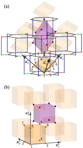
Figure 2: 3D network of the $\mathbb{Z}_{2}$ fluxes. (a) The hypernonagon lattice contains two types of closed volumes indicated by the orange and purple hexahedra. Both are constructed from the centers of the eight plaquettes, indicated by spheres. The numbers 1–8 indicate the plaquettes M₁–M₈ in Figs. 1(c)-1(e) on which the $\mathbb{Z}_{2}$ fluxes $W_{p}$ are defined. The spheres form a distorted cubic lattice. (b) The simple cubic lattice deformed from (a). ${\bf a}^{\prime}_{1}$, ${\bf a}^{\prime}_{2}$, and ${\bf a}^{\prime}_{3}$ in (a) [${\bf a}^{\prime\prime}_{1}$, ${\bf a}^{\prime\prime}_{2}$, and ${\bf a}^{\prime\prime}_{3}$ in (b)] are the primitive translation vectors for the deformed (simple) cubic lattice.

In fact, one can further simplify the lattice geometry when focusing on the elementary plaquettes. As shown in Figs. 1(c)-1(e), the lattice structure is composed of eight types of 9-site plaquettes in each unit cell, M₁–M₈. They form a closed volume as illustrated by the orange hexahedron in Fig. 2(a), where the numbered spheres represent the eight plaquettes in Figs. 1(c)-1(e). In addition to the orange hexahedron, one can find a second closed volume which spans across neighboring unit cells, illustrated by the purple hexahedron in Fig. 2(a). Note that the purple and orange inversion centers in Fig. 1(b) correspond to the centers of the purple and orange hexahedra, respectively. Importantly, these two types of hexahedra form a distorted cubic lattice, which can be further deformed to a simple cubic lattice as shown in Fig. 2(b) Kato et al. (2017, 2018).

II.2 Kitaev model and conserved $\mathbb{Z}_{2}$ fluxes

In the following, we will consider a standard Kitaev model

$$\mathcal{H}=-J_{x}\sum_{\langle i,j\rangle_{x}}\sigma_{i}^{x}\sigma_{j}^{x}-J_{y}\sum_{\langle i,j\rangle_{y}}\sigma_{i}^{y}\sigma_{j}^{y}-J_{z}\sum_{\langle i,j\rangle_{z}}\sigma_{i}^{z}\sigma_{j}^{z}\,,$$ (1)

where $\sigma_{i}^{x}$, $\sigma_{i}^{y}$, and $\sigma_{i}^{z}$ are the Pauli matrices describing a spin-$1/2$ degree of freedom at site $i$. The sum $\langle i,j\rangle_{\gamma}$ is taken over all the $\gamma$ bonds ($\gamma=x,y,z$, corresponding to three different types of bonds), and $J_{\gamma}$ is the exchange constant for the $\gamma$ bonds. Such a Kitaev model can be defined for any tricoordinated lattice, even in three spatial dimensions O’Brien et al. (2016). Doing so for the hypernonagon lattice at hand leads us to the assignment of $x,y,z$-bonds as illustrated in Fig. 1. Note that (up to permutations) there is exactly one such assignment of bonds that does not break any of the lattice symmetries discussed above.

Since we are particularly interested in the $\mathbb{Z}_{2}$ gauge physics of this 3D Kitaev model, we readily define an elementary $\mathbb{Z}_{2}$ flux for every plaquette M_p in analogy to Kitaev models on other lattice geometries as

$$W_{p}=\prod_{\langle i,j\rangle_{\gamma}\in{\rm M}_{p}}\sigma_{i}^{\gamma}\sigma_{j}^{\gamma}\,.$$ (2)

Here the product is taken for all the bonds comprising the plaquette in a clockwise manner if viewed from the inside of the orange hexahedron to which the plaquette belongs. All $W_{p}$ commute with one another and with the Hamiltonian, and $W_{p}^{2}=-1$ for all $p$. Hence, $W_{p}$ is a conserved quantity taking eigenvalues  of either $+{\mathrm{i}}$ or $-{\mathrm{i}}$. By using this fact, the Hamiltonian can be block diagonalized, and the Hilbert space of each block (flux sector) is labeled by its flux configuration $\{W_{p}\}=\{W_{1},W_{2},\cdots\}$.

In the present case of the hypernonagon lattice, the $\mathbb{Z}_{2}$ fluxes $W_{p}$ have two important features. One comes from the dimensionality of the lattice structure. As first discussed for the hyperhoneycomb lattice Mandal and Surendran (2009), $\{W_{p}\}$ is subject to local and global constraints in three dimensions. In particular, the local constraint, which enforces the product of $W_{p}$ on any closed volume to be $+1$, allows excitations by flipping $W_{p}$ only in the form of closed loops. This leads to a topological finite-$T$ phase transition between the high-$T$ paramagnet and the low-$T$ quantum spin liquid driven by a proliferation of excited loops Nasu et al. (2014a). This situation is common to any 3D Kitaev models; indeed, similar finite-$T$ phase transitions were found on other 3D lattices Mishchenko et al. (2017); Eschmann et al. (2019). In our hypernonagon case, the local constraint is enforced on each hexahedron in Fig. 2: the product of $W_{p}$ on the eight vertices is always equal to unity in all orange and purple hexahedra Kato et al. (2017).

The other important feature of $W_{p}$ is that it is composed of an odd number of sites for the hypernonagon lattice at hand. When the fluxes are defined for odd length loops, a pair of flux assignments with opposite signs of $W_{p}$ form a time-reversal pair Kitaev (2006). This allows for the possibility of CSLs where time-reversal symmetry is broken spontaneously by selecting a particular configuration of $W_{p}$. Indeed, on the triangle-honeycomb lattice, which consists of 3 and 12-site loops, the ground state of the Kitaev model was found to be a CSL Yao and Kivelson (2007). Furthermore, a finite-$T$ phase transition was found from the high-$T$ paramagnet to the low-$T$ CSL Nasu and Motome (2015).

Thus, our hypernonagon Kitaev model has at least two interesting possibilities for finite-$T$ phase transitions: one is a topological transition originating from the local constraints on $\{W_{p}\}$ and the other is the spontaneous breaking of time-reversal symmetry. Such possibilities were examined in the limits of strong anisotropy in the exchange interactions where finite-$T$ transitions to two different types of CSLs were found for the effective models. Both transitions have been found to be first order, with the simultaneous occurrence of the topological change associated with the ordering of the $\mathbb{Z}_{2}$ gauge structure and the concurrent breaking of a point-group symmetry of the lattice by nonuniform $\mathbb{Z}_{2}$ flux ordering Kato et al. (2017).

III Methods

To analyze the hypernonagon Kitaev model introduced in the previous section, we primarily employ numerical approaches to capture the $\mathbb{Z}_{2}$ gauge physics of the model: QMC simulations to access the finite-$T$ thermodynamics and variational calculations to map out the entire zero-$T$ phase diagram. These numerical approaches are complemented by analytical calculations of the Majorana band structures, which employ various tricks to identify their inherent topological features. In the following, we will briefly outline the relevant details of all three approaches.

III.1 Quantum Monte Carlo simulation at finite temperatures

The QMC simulations of the Kitaev model in Eq. (1) are based on a Majorana fermion representation of the spins Nasu et al. (2014a). Such a representation can be introduced via a Jordan-Wigner transformation on “chains” consisting of two types of bonds (e.g., the $y$ and $z$ bonds) Chen and Hu (2007); Feng et al. (2007); Chen and Nussinov (2008), followed by a rewriting in terms of the two types of Majorana fermions $c$ and $\bar{c}$, as

$$\mathcal{H}=\mathrm{i}J_{y}\sum_{\langle i,j\rangle_{y}}c_{i}c_{j}-\mathrm{i}J_{z}\sum_{\langle i,j\rangle_{z}}c_{i}c_{j}-\mathrm{i}J_{x}\sum_{\langle i,j\rangle_{x}}\eta_{ij}c_{i}c_{j}\,,$$ (3)

where the sums are taken for $i<j$, and $\eta_{ij}={\mathrm{i}}\bar{c}_{i}\bar{c}_{j}$. Thus, the Majorana fermions described by $c$ have an itinerant nature, while those described by $\bar{c}$ are localized on the $x$ bonds. Here, $\eta_{ij}$ is also a local conserved quantity taking eigenvalue either $+1$ or $-1$, which is related to $W_{p}$ in Eq. (2) as $W_{p}={\mathrm{i}}\prod_{\langle i,j\rangle_{x}\in p}\eta_{ij}$, where the product is taken for all the $x$ bonds included in the 9-site loop. This Majorana fermion representation enables us to perform sign-free QMC simulations by sampling configurations of the $\mathbb{Z}_{2}$ variables $\{\eta_{ij}\}$.

In the Monte Carlo (MC) sampling, we perform single flip updates of the $\mathbb{Z}_{2}$ variables $\{\eta_{ij}\}$ as well as replica exchange Hukushima and Nemoto (1996) updates with respect to $T$. In the single flip updates, we compute the Boltzmann weight difference caused by a local sign flip of $\eta_{ij}$ by employing the Green-function-based kernel polynomial method introduced in Refs. Weiße, 2009; Weiße et al., 2006 and applied to a Kitaev model in Ref. Mishchenko et al., 2017. The computational complexity of a single update is thereby reduced to $\mathcal{O}(N)$ (where $N$ is the number of sites), which is a big advantage compared to the $\mathcal{O}(N^{3})$ scaling of a naive approach based on exact diagonalizations of the Hamiltonian. In addition, replica exchange updates are introduced to prevent the system from freezing at low $T$. To enhance its overall efficiency, we adopt a feedback optimization Katzgraber et al. (2006) of the $T$ set for parallel tempering, which significantly speeds up thermal equilibration .

In the setup of our QMC simulations, we consider two clusters with a total of $N=12\times L^{3}$ sites: one has the linear dimension $L=4$ ($N=768$) and the other has $L=6$ ($N=2592$). We employ periodic boundary conditions in all spatial directions in order to minimize finite-size effects in our simulations . We optimize the $T$ set by the feedback optimization technique Katzgraber et al. (2006), where we initially perform $3000$ MC sweeps for sampling after $3000$ MC sweeps for thermalization, and then add $1000$ MC sweeps to both sampling and thermalization after each successive optimization iteration. We perform seven and four steps of the feedback optimization for the $L=4$ and $L=6$ systems, respectively, where, for the optimization of the $L=6$ system, we start from the $T$ set obtained from the fifth step for the $L=4$ system. We present the results at the sixth step ($4800$ MC samples) and the seventh step ($4000$ MC samples) for the $L=4$ system, and at the third step ($1600$ MC samples) and the fourth step ($4800$ MC samples) for the $L=6$ system. The measurements are performed after every MC sweep .

III.2 Variational calculations for the ground state

Probing several different configurations of the $\mathbb{Z}_{2}$ fluxes (see Sec. V), we obtain the corresponding energies by exact diagonalization of the Hamiltonian in Eq. (3). From the comparison, we determine the variational ground state as the state with the lowest energy for a given set of the exchange couplings, $J_{x}$, $J_{y}$, and $J_{z}$. The energy of a particular flux configuration $\{W_{p}\}$ is calculated by constructing the $\{\eta_{ij}\}$ configuration that reproduces the given $\{W_{p}\}$ and diagonalizing the Fourier transform of the Hamiltonian in Eq. (3) for the obtained $\{\eta_{ij}\}$. We note that $\{W_{p}\}$ for all the variational states are reproduced by a particular $\{\eta_{ij}\}$ within the $L=2$ unit cell. In these calculations, we consider a system with linear system size $L=48$.

III.3 Determination of the Majorana band structures

Given a variational flux configuration for a specific choice of the exchange couplings, the fermionic ground state is obtained by computing the corresponding spectrum of the itinerant Majorana fermions. In order to efficiently determine whether the fermionic quasiparticles are gapped or gapless at a given point in the phase diagram, the Berry curvature is integrated over 2D planes Fukui et al. (2005) which cut through the 3D Brillouin zone, i.e., by fixing one component of the momentum and integrating over the other two.

For those planes on which the fermionic spectrum is gapped, the result is a quantized Chern number. In a Weyl spin liquid Hermanns et al. (2015) phase, the Chern number jumps discontinuously as the plane passes through a Weyl node by an amount equal to the charge of that Weyl node – thereby allowing for a robust identification of the location of Weyl nodes in momentum space. In general, the Berry curvature is ill-defined for a plane on which the fermionic spectrum is gapless. In the case that there is a one-dimensional (1D) (line) or 2D (plane) nodal manifold, the result is a range of momentum values for which the Berry flux is ill-defined and typically fluctuates wildly.

With this information, it may be determined whether a given point in the phase diagram corresponds to a gapped or gapless fermionic spectrum. If the Berry flux is vanishing everywhere, the fermions must be gapped throughout the entire Brillouin zone. However, if at any point the Berry flux is nonzero – whether it takes a nonvanishing quantized Chern number or fluctuates wildly – the fermionic spectral gap must close somewhere. For the regions of the phase diagram where the gap closing occurs at a high-symmetry point, the resolution of the phase diagram data can be further increased by checking whether or not the gap closes at that point for a given choice of couplings.

Alongside this analysis, the projective symmetry group Wen (2002) is utilized to deduce general constraints on the gapless fermionic excitations, thereby explaining the distinct stable topology of the nodal manifold of the itinerant Majorana fermions appearing in the different CSL phases. The precise projective representation of physical symmetries of the model when written in the Majorana fermion representation determines the character of the nodal manifold O’Brien et al. (2016); Yamada et al. (2017). In particular, the projective symmetry group may enforce the stability of either fully 2D Fermi surfaces, nodal lines, Dirac cones or topological Weyl nodes.

IV Thermodynamics

We start our presentation of results by first discussing the thermodynamics of the hypernonagon Kitaev model.

IV.1 Thermal fractionalization

Figure 3 summarizes our QMC results for the isotropic Kitaev model with equal couplings $J_{x}=J_{y}=J_{z}$, normalized to $J_{x}+J_{y}+J_{z}=1$. It shows (a) the internal energy $\varepsilon$, (b) the specific heat $C$, and (c) the entropy $S$ per site as functions of $T$ at the last two optimization steps for each system size as described in Sec. III.1. In this resolution, the two results appear to overlap; we will discuss the convergence in Sec. IV.2. Similar to the previous works on other lattices Nasu et al. (2014a, 2015); Mishchenko et al. (2017), the specific heat $C$ of the Kitaev model on the hypernonagon lattice exhibits two peaks as shown in Fig. 3(b), corresponding to the steep changes of the energy $\varepsilon$ plotted in Fig. 3(a) [see the low-$T$ part in Fig. 4(a)]. One is a broad peak at $T\approx 0.5$ and the other is a sharp peak at $T\approx 0.0024$. The high-$T$ peak comes from the itinerant Majorana fermions $c$, while the low-$T$ peak is due to the $\mathbb{Z}_{2}$ fluxes, which are related to the localized Majorana fermions $\bar{c}$ Nasu et al. (2014a, 2015). This is clearly demonstrated by a decomposition of the specific heat $C$ into each contribution, as shown in Fig. 3(b) Dwivedi et al. (2018). Figure 3(c) demonstrates that half of the total entropy $S$, $\frac{1}{2}\ln 2\approx 0.347$, is released at each peak of the specific heat $C$ . This successive release of the entropy is a common feature to all Kitaev models, indicative of the thermal fractionalization of spins Nasu et al. (2015).

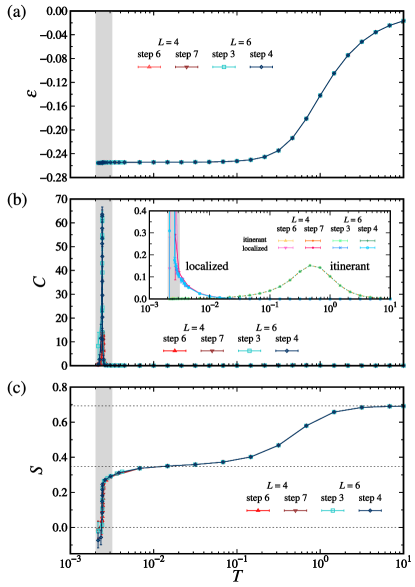
Figure 3: Thermodynamics of the hypernonagon Kitaev model obtained by QMC simulations for the isotropic exchange interactions $J_{x}=J_{y}=J_{z}=1/3$. Shown are the $T$ dependence of (a) the internal energy $\varepsilon$, (b) the specific heat $C$, and (c) the entropy $S$ per site at the last two optimization steps. The inset of (b) displays the decomposition into the contributions from the itinerant Majorana fermions and the localized $\mathbb{Z}_{2}$ fluxes. The data are calculated for the system sizes with $L=4$ and $L=6$. The gray area indicates the $T$ range plotted in Fig. 4. The dashed horizontal lines in (c) indicate $0$, $\frac{1}{2}\ln 2$, and $\ln 2$.

IV.2 Finite-temperature phase transition

In the following, we focus on the low-$T$ region where the specific heat $C$ shows a sharp peak (gray area in Fig. 3). Figure 4 displays the low-$T$ QMC data. The internal energy $\varepsilon$ suddenly drops at $T\approx 0.0024$, as shown in Fig. 4(a). The energy change becomes sharper for $L=6$ than $L=4$. Correspondingly, the specific heat $C$ shows a sharp peak, as shown in Fig. 4(b). We find that the peak height (width) becomes higher (narrower) for larger $L$, indicating a phase transition .

In order to clarify the nature of the phase transition, we calculate the histogram of the internal energy $\varepsilon$, $P(\varepsilon)$. The results are shown in Fig. 5. We find that the energy distribution bifurcates for both system sizes, while it has an additional structure in the low-energy part (we return to this point later). The bifurcation strongly suggests a first-order phase transition, which is consistent with the size dependence of the specific heat $C$, namely, the peak height increases roughly proportional to the system size as expected for a first-order phase transition.

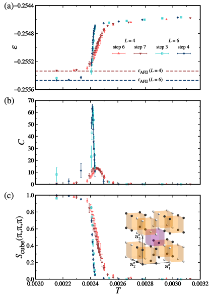
Figure 4: Low-$T$ phase transition. Shown are the $T$ dependence of (a) the internal energy $\varepsilon$ and (b) the specific heat $C$ as given in Figs. 3(a) and 3(b), respectively, but plotted on a linear $T$ scale, zooming in the low-$T$ regime (the gray areas in Fig. 3). (c) The order parameter for the $\mathbb{Z}_{2}$ flux ordering, $S_{\rm cube}(\textbf{Q})$ at $\textbf{Q}=(\pi,\pi,\pi)$ at the last two optimization steps. The inset of (c) indicates the flux configuration in the low-$T$ CSL phase, where black and white spheres represent fluxes with $W_{p}=+{\rm i}$ and $-{\rm i}$, respectively. $\varepsilon_{\rm AFII}$ in (a) indicates the ground state energy for each system size. See the main text for details.

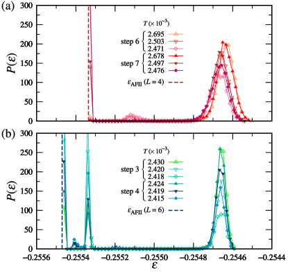
Figure 5: First-order nature of the thermal phase transition. Histograms of the internal energy $\varepsilon$, $P(\varepsilon)$, in the vicinity of the transition temperature $T_{c}=0.00244(4)$ obtained by QMC simulations for (a) $L=4$ and (b) $L=6$ at the last two optimization steps. $\varepsilon_{\rm AFII}$ is the internal energy calculated for the $W_{p}$ configuration in the AFII phase for each system size. See the text for details.

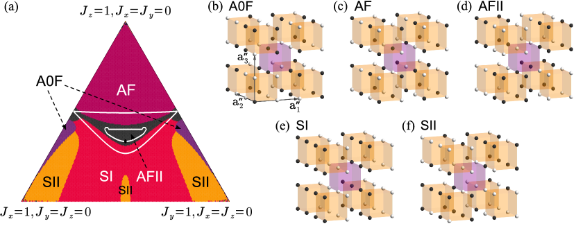
Figure 6: Ground state of the hypernonagon Kitaev model. (a) The ground state phase diagram in the parameter space $J_{x}+J_{y}+J_{z}=1$ ($J_{\gamma}\geq 0$) obtained by variational calculations. Each corner corresponds to the anisotropic limits where one of $J_{\gamma}=1$ and the other two are zero. The black dot at the center represents the isotropic case $J_{x}=J_{y}=J_{z}=1/3$. The white lines represent gapped/gapless boundaries with respect to the itinerant Majorana spectrum; the system has gapless excitations in the area sandwiched by the two closed white lines. Five distinct phases are found: A0F (purple), AF (magenta), AFII (gray), SI (red), and SII (yellow). The flux configurations are shown in (b)-(f) for each phase. The black and white spheres represent fluxes with $W_{p}=+{\mathrm{i}}$ and $-{\mathrm{i}}$, respectively. Since all the variational states have the same energy in the corners of the phase diagram, numerical noise may be seen close to them.

We find that the finite-$T$ phase transition is caused by ordering of the $\mathbb{Z}_{2}$ fluxes $W_{p}$. This can be monitored by the structure factor of $W_{p}$, defined in matrix form as

$$S^{\alpha\beta}_{\rm cube}(\textbf{k})=\frac{1}{8^{2}L^{3}}\langle W_{\alpha}(\textbf{k})\cdot[W_{\beta}(\textbf{k})]^{*}\rangle\,,$$ (4)

where

$$W_{\alpha}(\textbf{k})=\frac{1}{\sqrt{L^{3}}}\sum_{\textbf{r}}\mathrm{e}^{-\mathrm{i}\textbf{k}\cdot\textbf{r}}W_{\alpha}(\textbf{r})\,.$$ (5)

Here, r is the position vector for the orange hexahedral unit cell in Fig. 2(b) and $\alpha,\beta\in\{1,2,\ldots,8\}$ label the vertices of the hexahedron. We find that the structure factor develops a Bragg peak at $\textbf{k}=\textbf{Q}=(\pi,\pi,\pi)$, with all the matrix elements of $S^{\alpha\beta}_{\rm cube}(\textbf{Q})$ being equivalent. Hence, we define the order parameter $S_{\rm cube}(\textbf{Q})\equiv\sum_{\alpha,\beta}S^{\alpha\beta}_{\rm cube}(\textbf{Q})$ and plot its value as a function of $T$ in Fig. 4(c). The result indicates that the first-order transition of the system is caused by a spontaneous ordering of the $\mathbb{Z}_{2}$ fluxes where all fluxes in a given hexahedral unit have the same sign, while the units themselves form a staggered pattern. This is illustrated in the inset of Fig. 4(c). We call this flux order AFII (see Sec. V). As mentioned above, the ordering of $\{W_{p}\}$ corresponds to a spontaneous breaking of time-reversal symmetry. Hence, the transition observed here is deduced to occur from the high-$T$ paramagnetic phase to the low-$T$ quantum spin liquid phase with broken time-reversal symmetry, i.e., a CSL phase. In Fig. 4(a), we plot the ground state energy $\varepsilon_{\rm AFII}$ for this CSL phase for each $L$. Our QMC data quickly converge to these values below the transition $T$.

The peak $T$ of the specific heat $C$ does not change much from $L=4$ to $L=6$, as shown in Fig. 4(b). We estimate the transition $T$ to be $T_{c}=0.00244(4)$ so that both values are included in the error in the last digit, although more precise determination is necessary by the system-size extrapolation. We do not see any anomaly except at $T_{c}$ in the $T$ range studied here. This suggests that the hypernonagon Kitaev model at the isotropic point exhibits a single first-order transition to the CSL, similar to what is observed in its anisotropic limits Kato et al. (2017). However, given the peculiar structure of $P(\varepsilon)$ in Fig. 5, the possibility of multiple transitions within a very narrow $T$ range cannot be excluded at present, and needs to be examined carefully for larger system sizes. This is left for a future study.

In the 3D Kitaev models, the transition temperature $T_{c}$ is related to the loop tension, which defines the energy gap for a loop excitation of $W_{p}$ Kimchi et al. (2014); T. Eschmann et al. (2019). In our hypernonagon case, we estimate the flux gap, defined by the smallest excitation of a $W_{p}$ loop from the ground state, as $\Delta=0.0339(1)$. The previous studies for other 3D lattices showed that the ratio $T_{c}/\Delta$ is in the range of $\approx 0.11$–$0.15$ Nasu et al. (2014a); Mishchenko et al. (2017); T. Eschmann et al. (2019). In the hypernonagon case, however, the value of $T_{c}/\Delta\approx 0.07$ deviates from this trend: $T_{c}$ is considerably lower than the expected value given $\Delta$. The origin of the deviation can likely be traced back to the first-order nature of the transition in the hypernonagon lattice, where multiple symmetries (time-reversal and lattice point group) are broken simultaneously with the gauge ordering transition. In contrast, the transition for all other 3D Kitaev models appears to be continuous T. Eschmann et al. (2019), indicating that similar physics is at play as for the hyperhoneycomb and hyperoctagon cases for which the finite-$T$ transition has been shown to arise from a topological change of the loop-type excitations Nasu et al. (2014b, a); Mishchenko et al. (2017).

V Ground state phase diagram

Our calculations reveal several low-$T$ flux configurations when probing the phase diagram away from the isotropic coupling point, which all exhibit nonuniform arrangements of the $\mathbb{Z}_{2}$ fluxes. The five distinct arrangements are illustrated in Figs. 6(b)-6(f), which in the following we will refer to as A0F, AF, AFII, SI, and SII, respectively. Most of these were previously identified in certain parameter regimes, such as the SI configuration of Fig. 6(e) in initial studies O’Brien et al. (2016) of the hypernonagon model by using variational arguments, the A0F configuration of Fig. 6(b) in Ref. Kato et al., 2017, the SII configuration of Fig. 6(f) in the strong $J_{x}$ or $J_{y}$ limits Kato et al. (2017) with a subextensive degeneracy, and the AF configuration in the strong $J_{z}$ limit Kato et al. (2017). Only the AFII phase of Fig. 6(d) has hitherto remained unnoticed.

Using these five distinct ordering patterns as input for the variational calculations described in Sec. III.2, we can map out the entire zero-$T$ phase diagram of the $\mathbb{Z}_{2}$ flux sector for arbitrary Kitaev couplings. The result is summarized in Fig. 6(a) for the plane of $J_{x}+J_{y}+J_{z}=1$ with $J_{\gamma}\geq 0$ (with the phase diagram remaining the same when flipping the signs of all $J_{\gamma}$). In the phase diagram we find the AFII phase (gray area) around the isotropic point (black dot), consistent with our QMC results. When increasing $J_{z}$ (moving upwards in the phase diagram), the AFII phase gives way to an AF phase (magenta). On the other hand, when decreasing $J_{z}$ we find the SI phase (red), and finally the SII phase (yellow) at the bottom center as well as near the two bottom corners of the phase diagram. We also find narrow regions of the A0F phase (purple) near the edges of $J_{x}=0$ or $J_{y}=0$. We note that our results around the three corners are indeed consistent with ealier results Kato et al. (2017), derived perturbatively for the three anisotropic limits.

In addition to the phase boundaries arising from the $\mathbb{Z}_{2}$ flux ordering, we also determine the boundaries that arise from the transition between gapless and gapped band structures of the itinerant Majorana fermions – as indicated by the white lines in the phase diagram of Fig. 6(a). We find that in general these boundaries do not precisely coincide with the phase boundaries between the different flux patterns, i.e., for a given flux pattern there are regions where the Majorana spectrum is either gapped or gapless. In particular, the extent of the gapless region of the Majorana band structure corresponds to the region sandwiched by the two closed white lines in the phase diagram of Fig. 6(a). It is thus that the SI, AF, and AFII phases all have both gapped and gapless Majorana spectra, whereas for the A0F and SII phases the Majorana spectrum remains fully gapped for all parameters. We note that the isotropic point is right on the gapped/gapless boundary.

In the following sections, the nature of the gapless regions are discussed for the SI, AF, and AFII phases in further detail. As the lattice symmetries relevant to this discussion are the $C_{3}$-rotational, mirror, and inversion symmetries, the corresponding symmetry information for the different CSL flux phases is summarized in Table 1. Among the flux phases which host gapless fermions, only the SI phase breaks the rotational symmetry and two out of the three mirror symmetries. While the SI and AF phases respect inversion symmetry for all inversion centers, the AFII phase breaks inversion symmetry for the inversion centers corresponding to the orange hexahedra [see Fig. 6(d)]. In addition as discussed in Sec. II.2, by virtue of the hypernonagon lattice being non-bipartite, all flux configurations necessarily break time-reversal symmetry. For the AFII phase, however, the combination of time-reversal with the broken inversion symmetry operation is seen to yield a symmetry of the Hamiltonian.

Flux phase		$C_{3}$		Mirror planes		Inversion (purple / orange)
A0F		Yes		3		Yes / No
AF		Yes		3		Yes / Yes
AFII		Yes		3		Yes / No
SI		No		1		Yes / Yes
SII		No		1		No / No

Table 1: Overview of lattice symmetries for the different CSL phases. The relevant symmetries include $C_{3}$-rotational symmetry, the number of remaining mirror planes (for $J_{x}=J_{y}$) and whether inversion symmetries (corresponding to the purple and orange hexahedra) are present.

The physical inversion symmetry for all the CSL phases discussed here is represented projectively as

$$H(\textbf{k})=G^{\dagger}_{\mathcal{P}}~{}U^{\phantom{\dagger}}_{\mathcal{P}}~{}H(-\textbf{k})~{}U^{\dagger}_{\mathcal{P}}~{}G^{\phantom{\dagger}}_{\mathcal{P}},$$ (6)

where $U_{\mathcal{P}}$ is the matrix representation of the inversion operator acting on the unit cell and $G_{\mathcal{P}}$ is the associated $\mathbb{Z}_{2}$ gauge transformation. Note that for all the phases at hand, inversion symmetry is implemented trivially, i.e., with a uniform gauge transformation $G_{\mathcal{P}}$. A nonuniform gauge transformation necessitates a translation of $\mathbf{k}$ by half a reciprocal lattice vector on the right side of Eq. (6) O’Brien et al. (2016). The relevant energy relations are, thus, given by

$$E_{\alpha}(\textbf{k})=-E_{\beta}(-\textbf{k})\quad{\rm and}\quad E_{\alpha}(\textbf{k})=E_{\gamma}(-\textbf{k}),$$ (7)

due to particle-hole and inversion symmetry, respectively. Here $\alpha$, $\beta$, and $\gamma$ denote band indices.

V.1 SI phase

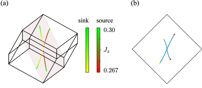
Figure 7: Gapless SI phase. (a) Evolution of Weyl nodes for coupling constants $0.267\leq J_{z}\leq 0.30$ with $J_{x}=J_{y}=(1-J_{z})/2$. The sink and source indicate the negatively- and positively-charged Weyl nodes, respectively. The shaded region indicates the remaining mirror plane in the SI phase with $J_{x}=J_{y}$. (b) Corresponding Fermi arcs on the 001-surface Brillouin zone for $(J_{x},J_{y},J_{z})=(0.36,0.36,0.28)$.

In the SI phase, the presence of trivially-implemented projective inversion symmetries prohibits the formation of stable Fermi surfaces due to the corresponding energy relation in Eq. (7) Hermanns and Trebst (2014). Furthermore, the absence of time-reversal symmetry prohibits the formation of stable nodal lines seen in some other Kitaev spin liquids, e.g., on the hyperhoneycomb lattice O’Brien et al. (2016), where such nodal lines are stabilized by a 1D winding number Burkov et al. (2011); Zhao and Wang (2013); Matsuura et al. (2013) associated with sublattice symmetry, i.e. a combination of trivially-implemented time-reversal and particle-hole symmetry. However, the combination of particle-hole and inversion symmetries allows for the presence of topologically protected Weyl nodes pinned to zero energy.

Indeed, diagonalizing the concrete Hamiltonian in the SI phase reveals an extended gapless Weyl spin liquid phase. Restricting the exchange couplings to the line $J_{x}=J_{y}=(1-J_{z})/2$, the gapless portion of the SI phase runs from $J_{z}\approx 0.267$, where the gap closes, to $J_{z}\approx 0.3$, where the ground state switches from the SI phase to the AFII phase. For $J_{z}\approx 0.267$, two positively-charged and two negatively-charged Weyl nodes simultaneously appear at the $\Gamma$ point of the Brillouin zone. As $J_{z}$ is further increased, the Weyl nodes split apart. For $J_{x}=J_{y}$, the Weyl nodes are pinned to the single mirror plane which is not broken in the SI phase.

Figure 7(a) shows the evolution of the Weyl nodes in the 3D Brillouin zone as the exchange couplings are varied for $0.276\leq J_{z}\leq 0.30$ with $J_{x}=J_{y}=(1-J_{z})/2$. The trajectory of negatively-charged Weyl nodes changes color from yellow to green as $J_{z}$ is increased, whereas the trajectory of positively-charged Weyl nodes changes from red to green. The corresponding Fermi arcs at the 001-surface Brillouin zone for $(J_{x},J_{y},J_{z})=(0.36,0.36,0.28)$ are plotted in Fig. 7(b).

V.2 AF phase

In the AF phase, as for the SI phase discussed above, the presence of trivially-implemented projective inversion symmetries prohibits the formation of stable Fermi surfaces. Furthermore, the absence of time-reversal symmetry prevents the formation of nodal lines protected by sublattice symmetry as mentioned above. However, the combination of particle-hole and inversion symmetries allows for the presence of topologically protected Weyl nodes pinned to zero energy.

Indeed, diagonalizing the concrete Hamiltonian in the AF phase reveals an extended region with Weyl nodes. Restricting the exchange couplings to the line $J_{x}=J_{y}=(1-J_{z})/2$, the gapless portion of the AF phase runs from $J_{z}\approx 0.42$, where the ground state switches from the AFII phase to the AF phase, to $J_{z}\approx 0.491$, where the Weyl nodes gap out. For $0.42<J_{z}\lesssim 0.491$, two oppositely-charged Weyl nodes are pinned to the $C_{3}$-invariant axis. As $J_{z}$ is increased, the two Weyl nodes move towards each other until they eventually meet at the $\Gamma$ point for $J_{z}\approx 0.491$ and mutually annihilate.

Figure 8: Gapless AF phase. (a) Evolution of Weyl nodes for coupling constants $0.42\leq J_{z}\leq 0.491$ with $J_{x}=J_{y}=(1-J_{z})/2$. The sink and source indicate the negatively- and positively-charged Weyl nodes, respectively. (b) Corresponding Fermi arc in the 001-surface Brillouin zone for $(J_{x},J_{y},J_{z})=(0.27,0.27,0.46)$ denoted in blue. Additional surface states are marked in red and are discussed in Appendix B.

Figure 8(a) shows the evolution of the Weyl nodes in the 3D Brillouin zone as the exchange couplings are varied for $0.42\leq J_{z}\leq 0.491$ with $J_{x}=J_{y}=(1-J_{z})/2$. The trajectory of negatively-charged Weyl nodes (sinks) changes color from yellow to green as $J_{z}$ is increased, whereas the trajectory of positively-charged Weyl nodes (sources) changes from red to green. The corresponding Fermi arc at the 001-surface of the Brillouin zone for $(J_{x},J_{y},J_{z})=(0.27,0.27,0.46)$ is plotted in blue in Fig. 8(b).

In addition to the Fermi arc which terminates at the projection of the Weyl nodes in the surface Brillouin zone, there appear additional line-like surface states which form incontractible loops. These can be seen as remnants of Fermi arcs due to the Weyl nodes which are gapped out in this part of the phase diagram. For a thorough discussion of these additional surface states, we refer to Appendix B.

V.3 AFII phase

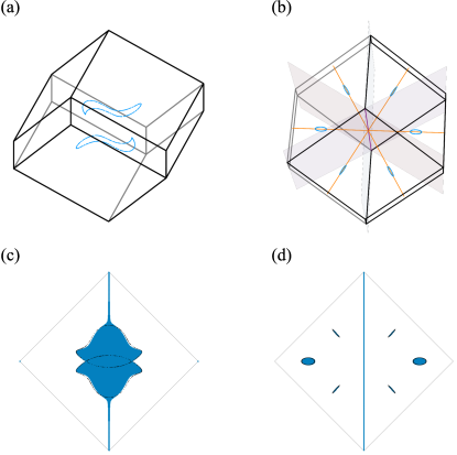
Figure 9: Gapless AFII phase. (a) Nodal lines for $(J_{x},J_{y},J_{z})=(0.34,0.34,0.32)$ shown in blue. (b) Nodal lines for $(J_{x},J_{y},J_{z})=(0.3035,0.3035,0.393)$ shown in blue. The shaded planes denote the three mirror invariant planes, whereas the orange lines denote the k points invariant under a combination of mirror and inversion symmetries. (c) and (d) Surface states for $J_{z}=0.32$ and $J_{z}=0.393$, respectively, depicted in blue along with projections of bulk nodal lines depicted in black for the 001-surface Brillouin zone.

In the AFII phase, as for the SI and AF phases, the presence of a trivially-implemented inversion symmetry prohibits the formation of stable Fermi surfaces. Furthermore, like for the SI phase, the absence of time-reversal symmetry prevents the formation of nodal lines protected by sublattice symmetry.

However, it has been shown that in a system where the combination of inversion and time-reversal symmetries is preserved, one may define both 1D and 2D $\mathbb{Z}_{2}$ winding numbers Kim et al. (2015); Fang et al. (2015). The 1D winding number corresponds to a Berry phase of either 0 or $\pi$ acquired upon traversal of a 1D loop. It may stabilize nodal lines similarly to what has been seen for time-reversal invariant Kitaev spin liquids, e.g., on the hyperhoneycomb lattice O’Brien et al. (2016). Additionally, pairs of nodal lines can be stabilized by the presence of a 2D $\mathbb{Z}_{2}$ winding number, i.e., a nodal line may carry a $\mathbb{Z}_{2}$ monopole charge Fang et al. (2015). Due to their monopole charges, such nodal lines must always be created and annihilated in pairs rather than being continuously deformed to a point and gapped out in isolation. Crucially, inversion and time-reversal symmetries need not individually be preserved in the system, only the combination of the two. For the hypernonagon lattice, any fixed flux sector breaks time-reversal symmetry spontaneously. However, in the AFII phase where one of the inversion symmetries is broken, the combination of the corresponding inversion operation with time-reversal indeed yields a symmetry of the Hamiltonian. In this case, line nodes can be stabilized even in the absence of sublattice symmetry.

Diagonalizing the concrete Hamiltonian in the AFII phase reveals an extended gapless region with nodal lines. Restricting the exchange couplings to the line $J_{x}=J_{y}=(1-J_{z})/2$, the gapless portion of the AFII phase runs from $J_{z}\approx 0.3$, where the ground state switches from the SI phase to the AFII phase, to $J_{z}\approx 0.42$, where the ground state switches from the AFII phase to the AF phase, with a region in between $1/3<J_{z}\lesssim 0.392$ for which the spectrum is fully gapped.

At the isotropic point $J_{z}=1/3$ there is a fourfold degeneracy at zero energy at the $\Gamma$ point which gaps out as soon as $J_{z}$ is increased. However, for $J_{z}<1/3$, this fourfold degeneracy is split into two nodal lines which grow larger and move away from each other as $J_{z}$ is increased further [see Fig. 9(a)]. Artificially extending the analysis of the AFII flux configuration for $J_{z}\lesssim 0.3$, where there is a phase transition to the SI phase, the nodal lines can be seen to wrap around the Brillouin zone before meeting once more and mutually annihilating at $J_{z}\approx 0.22$. Putting the system on a slab geometry, one finds both “drumhead” surface states Burkov et al. (2011); Phillips and Aji (2014); Chiu and Schnyder (2014); Chen et al. (2015); Mullen et al. (2015); Wawrzik et al. (2018) filling the projection of the nodal lines to the surface Brillouin zone as well as Fermi arc surface states connecting the two projections [see Fig. 9(c)]. The latter suggests that the nodal lines carry a $\mathbb{Z}_{2}$ monopole charge Gorbar et al. (2015a, b).

For the gapless region corresponding to $J_{z}\gtrsim 0.392$, a number of nodal lines are stabilized by a 1D $\mathbb{Z}_{2}$ winding number. For $J_{z}\approx 0.392$, a total of six nodal points appear along high-symmetry lines related to one another by inversion and mirror symmetries or, equivalently, by $C_{3}$ and inversion symmetries. The high-symmetry lines themselves correspond to momenta invariant under the combination of mirror and inversion symmetries – one such line for each of the three mirror planes [see Fig. 9(b)]. As $J_{z}$ is increased, the point nodes immediately expand to nodal lines which move through the Brillouin zone and are heavily deformed. Figure 9(b) shows these nodal lines for $J_{z}=0.393$. Due to the severe deformation of the nodal lines, the figure shows a “top” view from which the deformation is significantly less evident.

Putting the model on a slab geometry [see Figs. 9(c) and 9(d)], there are seen to be drumhead-type surface states filling the projection of the nodal lines to the surface Brillouin zone as well as the remnant of a Fermi arc from the $\mathbb{Z}_{2}$ monopole nodal lines which appear in another part of the phase diagram as discussed above. However, no Fermi arc like states are observed connecting the disjoint projections of the bulk nodal lines. The lack of such Fermi arc surface states along with the fact that the bulk nodal lines are not created and destroyed in pairs, rather they appear individually at arbitrary points in the Brillouin zone, indicates that they carry a 1D winding number rather than the 2D monopole charge.

VI Concluding remarks

To summarize, we have explored the physics arising from the crystalline ordering of the $\mathbb{Z}_{2}$ fluxes in the hypernonagon Kitaev model. The three-dimensionality of the lattice in combination with existence of odd-length plaquettes gives a potential for at least two types of finite-$T$ phase transitions – a topological one originating from loop proliferation of the $\mathbb{Z}_{2}$ flux excitations and the spontaneous breaking of time-reversal symmetry leading to a CSL. In addition, a previous study has suggested the breaking of additional point-group symmetries of the lattice by nonuniform ordering of the $\mathbb{Z}_{2}$ fluxes. Motivated to find such unconventional finite-$T$ phase transitions beyond the Landau-Ginzburg-Wilson description, we have employed large-scale, sign-free QMC simulations on the basis of the kernel polynomial method. While our numerics found a single phase transition, at which time-reversal and lattice symmetries are simultaneously broken, the transition itself turns out to be strongly first order in nature. Further exploring the zero-temperature physics of the model, we have established the presence of five distinct nonuniform crystalline $\mathbb{Z}_{2}$ flux orderings, all of which except for one are not commensurate with the underlying symmetries of the hypernonagon lattice. In addition, we calculated the band structures of the itinerant Majorana fermions for all the flux orderings. We found that in the three phases the itinerant Majorana fermions form both gapped and gapless excitation spectra, and this gapped/gapless boundary does not necessarily coincide with the boundaries between the different flux phases. Finally, we clarified the topological nature of the itinerant Majorana band structures by identifying topological features such as Weyl nodes or nodal lines which are accompanied by topologically protected surface states, Fermi arcs and drumhead states correspondingly.

Appendix A Lattice Information

As mentioned in Sec. II.1, it is possible to define an equivalent, but deformed version of the hypernonagon lattice in terms of honeycomb layers joined by mid-bond sites [see Fig. 1(b)]. The concrete choice of elementary unit cell for this deformed lattice has twelve sites with positions given by

$$\begin{matrix}[l]\mathbf{r}_{1}=\left(-\frac{2}{\sqrt{3}},0,0\right),&\mathbf{r}_{2}=\left(-\frac{7}{4\sqrt{3}},\frac{1}{4},0\right),\\ \\ \mathbf{r}_{3}=\left(-\frac{7}{4\sqrt{3}},\frac{1}{4},\frac{1}{\sqrt{3}}\right),&\mathbf{r}_{4}=\left(-\frac{\sqrt{3}}{2},\frac{1}{2},\frac{1}{\sqrt{3}}\right),\\ \\ \mathbf{r}_{5}=\left(-\frac{1}{2\sqrt{3}},-\frac{1}{2},0\right),&\mathbf{r}_{6}=\left(-\frac{1}{\sqrt{3}},-\frac{1}{2},0\right),\\ \\ \mathbf{r}_{7}=\left(-\frac{1}{\sqrt{3}},-\frac{1}{2},\frac{1}{\sqrt{3}}\right),&\mathbf{r}_{8}=\left(-\frac{\sqrt{3}}{2},-\frac{1}{2},\frac{1}{\sqrt{3}}\right),\\ \\ \mathbf{r}_{9}=\left(-\frac{1}{2\sqrt{3}},\frac{1}{2},0\right),&\mathbf{r}_{10}=\left(-\frac{1}{4\sqrt{3}},\frac{1}{4},0\right),\\ \\ \mathbf{r}_{11}=\left(-\frac{1}{4\sqrt{3}},\frac{1}{4},\frac{1}{\sqrt{3}}\right),&\mathbf{r}_{12}=\left(0,0,\frac{1}{\sqrt{3}}\right).\end{matrix}$$ (8)

The lattice vectors are chosen to be

$$\begin{matrix}[l]\mathbf{a}^{\prime}_{1}=\left(-\frac{\sqrt{3}}{2},\frac{1}{2},\frac{1}{\sqrt{3}}\right),&\mathbf{a}^{\prime}_{2}=\left(0,-1,\frac{1}{\sqrt{3}}\right),\\ \\ \mathbf{a}^{\prime}_{3}=\left(\frac{\sqrt{3}}{2},\frac{1}{2},\frac{1}{\sqrt{3}}\right)\end{matrix}$$ (9)

with corresponding reciprocal lattice vectors

$$\begin{matrix}[l]\mathbf{q}^{\prime}_{1}=\left(-\frac{2\pi}{\sqrt{3}},\frac{2\pi}{3},\frac{2\pi}{\sqrt{3}}\right),&\mathbf{q}^{\prime}_{2}=\left(0,-\frac{4\pi}{3},\frac{2\pi}{\sqrt{3}}\right),\\ \\ \mathbf{q}^{\prime}_{3}=\left(\frac{2\pi}{\sqrt{3}},\frac{2\pi}{3},\frac{2\pi}{\sqrt{3}}\right).\end{matrix}$$ (10)

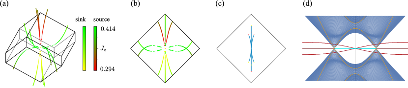
Figure 10: Evolution of Weyl nodes for coupling constants $0.294\leq J_{z}\leq 0.414$ with $J_{x}=J_{y}=(1-J_{z})/2$ in (a) the bulk Brillouin zone and (b) projected down to the 001-surface Brillouin zone, respectively. The two Weyl nodes on the $C_{3}$-invariant axis are not shown for clarity. (c) Corresponding Fermi arcs in the 001-surface Brillouin zone for $(J_{x},J_{y},J_{z})=(0.345,0.345,0.31)$. This includes the Weyl nodes which lie on the $C_{3}$-invariant axis along with their corresponding Fermi arc. (d) Band structures for $J_{z}=0.46$. The bulk band structure along the $C_{3}$-invariant axis is plotted in yellow showing the two Weyl nodes. The band structure for the slab geometry along the projection of the $C_{3}$ axis to the surface Brillouin zone is plotted in blue and red. The projection of the two Weyl nodes as well as the Fermi arc which connects them are colored blue. The bands responsible for the remaining surface states left over from the other Weyl nodes, which are gapped out for $J_{z}\approx 0.414$, are colored red.

The assignment of $x$, $y$ and $z$ bonds is depicted in Fig. 1(b) corresponding to red, green and blue colored bonds, respectively. Up to permutations of the bond types, this assignment is unique. All $x$ and $y$ bonds are related by a combination of $C_{3}$ and mirror symmetries. There are two distinct sets of $z$ bonds which are not related by lattice symmetries, however, all bonds of a given set may be mapped onto each other by a $C_{3}$ symmetry. The symmetry between $x$ and $y$ bonds is reflected in the ground state phase diagrams of Fig. 6(a).

Appendix B Surface states in the AF phase

As mentioned in the discussion of the AF phase in the main text, in addition to the Fermi arc which terminates at the projection of the Weyl nodes in the surface Brillouin zone, there appear additional line-like surface states which form incontractible loops. These can be seen as remnants of Fermi arcs due to Weyl nodes which are gapped out in this part of the phase diagram. If the flux configuration corresponding to the AF phase is artificially extended beyond its range of validity, i.e., for $J_{z}\lesssim 0.42$ with $J_{x}=J_{y}$, one finds the existence of an additional six Weyl nodes. These Weyl nodes emerge from the $\Gamma$-point at $J_{z}\approx 0.294$ and move away from one another as $J_{z}$ is increased, always pinned to the three mirror planes. At $J_{z}\approx 0.414$, the six Weyl nodes once again meet and annihilate at the $\Gamma$-point. However, as they do so, they trace out incontractible loops across the Brillouin zone. The evolution (excluding the two Weyl nodes on the $C_{3}$-invariant axis mentioned in the previous paragraph) in the bulk Brillouin zone as well as projected down to the 001-surface Brillouin zone, is depicted in Figs. 10(a) and (b), respectively.

A consequence of the trajectories of the Weyl nodes through the Brillouin zone is that their corresponding Fermi arcs [pictured in Fig. 10(c)], rather than shrinking to a point and gapping out with the Weyl nodes, are stretched out along similar incontractible loops. The result is that, while the Weyl nodes responsible for the surface states gap out, the surface states themselves remain behind [as can be seen in Fig. 8(b) of the main text]. Pictured in Fig. 10(d) is a composite of the bulk and slab geometry band structures for $J_{z}=0.46$ computed along the $C_{3}$-invariant axis and its projection to the 001-surface Brillouin zone, respectively. Here can be seen the Fermi arcs in blue which terminate at the projection of the Weyl nodes to the surface Brillouin zone at which point they dive back into the bulk. In red, however, are pictured the remnant surface bands from the Weyl nodes which have been gapped out. These bands are seen to be entirely disconnected from the bulk band structure.