A Narrow-stencil finite difference method for approximating viscosity solutions of fully nonlinear elliptic partial differential equations with applications to Hamilton-Jacobi-Bellman equations

Abstract

This paper presents a new narrow-stencil finite difference method for approximating the viscosity solution of second order fully nonlinear elliptic partial differential equations including Hamilton-Jacobi-Bellman equations. The proposed finite difference method naturally extends the Lax-Friedrichs method for first order problems to second order problems by introducing a key stabilization and guiding term called a “numerical moment”. The numerical moment uses the difference of two (central) Hessian approximations to resolve the potential low-regularity of viscosity solutions. It is proved that the proposed scheme is well posed (i.e, it has a unique solution) and stable in both the $\ell^{2}$-norm and the $\ell^{\infty}$-norm. The highlight of the paper is to prove the convergence of the proposed scheme to the viscosity solution of the underlying fully nonlinear second order problem using a novel discrete comparison argument. This paper extends the one-dimensional analogous method of [14] to the higher-dimensional setting. Numerical tests are presented to gauge the performance of the proposed finite difference methods and to validate the convergence result of the paper.

1 Introduction

This paper develops and analyzes a narrow-stencil finite difference approximation of the viscosity solution to the following fully nonlinear second order Dirichlet boundary value problem:

(1a) $$F[u](\mathbf{x})\equiv F\left(D^{2}u,\nabla u,u,\mathbf{x}\right) =0, \qquad\forall\mathbf{x}\in\Omega,$$

(1b) $$u(\mathbf{x}) =g(\mathbf{x}), \qquad\forall\mathbf{x}\in\partial\Omega,$$

where $\Omega\subset\mathbb{R}^{d}$ ($d\geq 2$) is a bounded domain and $D^{2}u(\mathbf{x})$ denotes the Hessian matrix of $u$ at $\mathbf{x}$. The PDE operator $F$ is a fully nonlinear second order differential operator in the sense that $F$ is nonlinear in $D^{2}u$ (or in at least one of its components). We assume $g$ is continuous and $F$ is Lipschitz in its first three arguments. Moreover, $F$ is assumed to be elliptic and satisfy a comparison principle (defined in Section 2.3). The paper focusses on a particular class of fully nonlinear PDEs called Hamilton-Jacobi-Bellman (HJB) equations which correspond to $F[u]=H[u]$, where

(2a) $$H[u] \equiv\min_{\theta\in\Theta}\bigl{(}L_{\theta}u-f_{\theta}\bigr{)},$$

(2b) $$L_{\theta}u =A^{\theta}(\mathbf{x}):D^{2}u+b^{\theta}(\mathbf{x})\cdot\nabla u+c^{\theta}(\mathbf{x})\,u.$$

HJB equations arise in various applications including stochastic optimal control, game theory, and mathematical finance (cf. [15]).

Numerical fully nonlinear PDEs has experienced some rapid developments in recent years. Various numerical methods have been proposed and tested (cf. [12, 23] and the references therein). In order to guarantee convergence to the viscosity solution of problem (1), most of these works follow the framework laid out by Barles-Souganidis in [1] which requires that a numerical scheme be monotone, consistent, and stable. It follows from a well-known result of [22] that, in general, monotone schemes are necessarily wide-stencil schemes as seen in [9, 10, 26, 29]. Consequently, to design convergent narrow-stencil schemes, one has to abandon the standard monotonicity requirement (in the sense of Barles-Souganidis [1]) and, instead, deal with non-monotone schemes. This in turn prohibits one to directly use the powerful and handy Barles-Souganidis (analysis) framework. On the other hand, it should be pointed out that monotone narrow-stencil schemes could be constructed for problem (1) in special cases. For example, when the matrix $A^{\theta}$ is diagonally dominant for all $\theta$, the methods proposed in [20, 2] become narrow-stencil schemes even though they require wide-stencils for general negative semi-definite matrices $A^{\theta}$. For isotropic coefficient matrices $A^{\theta}$ (i.e., $A^{\theta}$ diagonal), a monotone linear finite element method was proposed in [18]. Finally, we also mention that when $A^{\theta}$ satisfies a Cordes condition, a least square-like interior penalty discontinuous Galerkin (IP-DG) method was proposed in [30]. This method is obviously a narrow-stencil scheme, and it was proved to be convergent even though it is not monotone.

The primary goal of this paper is to develop a convergent narrow-stencil finite difference method for problem (1) in the general case when $F$ is uniformly elliptic. Thus, we only require $A^{\theta}$ to be uniformly negative definite as long as the underlying PDE satisfies the comparison principle. The method to be introduced in this paper can be regarded as a high dimensional extension of the one-dimensional finite difference method developed and analyzed by the authors in [14]. We note that this extension is far from trivial in terms of both method design and convergence analysis because of the additional difficulties caused by the second order mixed derivatives on the off-diagonal entries of the Hessian matrix $D^{2}u$ for $d\geq 2$. Indeed, constructing “correct” finite difference discretizations for those mixed derivatives and controlling their “bad” effect in the convergence analysis poses some significant new challenges. Recall that the main reason to use wide-stencils in the works cited above is exactly to “correctly” approximate the second order mixed derivatives. Hence, the new challenges which must be dealt with in this paper can be regarded as the price we need to pay for not using wide-stencils.

To achieve our goal, several key ideas are introduced and utilized in this paper. First, we introduce multiple discrete approximations of $\nabla u$ and $D^{2}u$ to locally capture the behavior of the underlying function $u$ when it has low regularity. The reason for using such multiple approximations is to compensate for the low resolution of a fixed grid, especially when using a narrow-stencil finite difference approximation. Second, as explained above, using narrow-stencils forces us to abandon the hope of constructing monotone finite difference schemes (again, in the sense of Barles-Souganidis [1]). However, in order to obtain a convergent scheme, the anticipated finite difference method must have some “good” structures. Our key motivating idea is to impose such a structure, called generalized monotonicity, on our finite difference scheme. We shall demonstrate that besides allowing for the use of narrow-stencils, generalized monotonicity is a more natural concept/structure than the usual monotonicity concept/structure, and it is much easier to verify. Third, to obtain practical generalized monotone finite difference methods, two important questions to answer are: how to build such a scheme and what is the primary mechanism that makes the method work? Inspired by the vanishing moment method developed in [11, 13], we propose a higher order stabilization term/mechanism, called a numerical moment, as a means to address these questions. We will see that the stabilization term/mechanism is the key for us to overcome the lack of monotonicity in the admissibility, stability, and convergence analysis.

The remainder of this paper is organized as follows. In Section 2 we introduce the basics of viscosity solution theory and elliptic operators as well as the corresponding notation. We also define our primary finite difference operators that will be used throughout the paper and list some identities for those difference operators. In Section 3 we first formulate our finite difference method and then prove several properties of the scheme. Section 4 is devoted to studying the well-posedness of the scheme. A contraction mapping technique based on a pseudo-time explicit Euler scheme is employed to prove the existence and uniqueness for the proposed finite difference scheme and to derive an $\ell^{2}$-norm stability estimate. In Section  5, an $\ell^{2}$-norm stability estimate for the second-order central difference quotients of the numerical solution is first derived using a Sobolev iteration technique. Then an $\ell^{\infty}$-norm stability estimate is derived based on combining both $\ell^{2}$ estimates. The results in Sections 4 and 5 rely upon some auxiliary linear algebra results that can be found in Appendix A. In Section 6 we present a detailed convergence analysis for the proposed finite difference method. In Section 7 we provide some numerical experiments that validate and complement the theory. The paper is concluded in Section 8 with a brief summary and some final remarks.

2 Preliminaries

We begin by recalling the viscosity solution concept for problem (1) as documented in [6, 8, 5] and defining basic difference operators that will be used to construct our finite difference method. We define the relevant function space notation in Section 2.1, state the definition of viscosity solutions in Section 2.2, and recall the definition of ellipticity and the comparison principle in Section 2.3. The comparison principle ensures uniqueness of solutions to (1). The specific assumptions for HJB equations will be given in Section 2.4. Lastly, in Section 2.5, we define our basic difference operators which will serve as the building blocks for constructing various discrete gradient and Hessian operators. The discrete gradient and Hessian operators will be used to define our narrow-stencil finite difference method in Section 3.

2.1 Function spaces and notation

Standard function and space notation as in [4] and [16] will be adopted in this paper. For example, for a bounded open domain $\Omega\subset\mathbb{R}^{d}$, $B(\Omega)$, $USC(\Omega)$, and $LSC(\Omega)$ are used to denote, respectively, the spaces of bounded, upper semicontinuous, and lower semicontinuous functions on $\Omega$. For any $v\in B(\Omega)$, we define

$$v^{*}(\mathbf{x})\equiv\limsup_{\mathbf{y}\to\mathbf{x}}v(\mathbf{y})\qquad\mbox{and}\qquad v_{*}(\mathbf{x})\equiv\liminf_{y\to\mathbf{x}}v(\mathbf{y}).$$

Then, $v^{*}\in USC(\Omega)$ and $v_{*}\in LSC(\Omega)$, and they are called the upper and lower semicontinuous envelopes of $v$, respectively. We also let $\mathcal{S}^{d\times d}\subset\mathbb{R}^{d\times d}$ denote the set of symmetric real-valued matrices.

In presenting the relevant viscosity solution concept for fully nonlinear second order PDEs, we shall use $G$ to denote a general fully nonlinear second order operator. More precisely, $G:\mathcal{S}^{d\times d}\times\mathbb{R}^{d}\times\mathbb{R}\times\overline{\Omega}\to\mathbb{R}$. The general second order fully nonlinear PDE problem is to seek a locally bounded function $u:\overline{\Omega}\to\mathbb{R}$ such that $u$ is a viscosity solution of

(3) $$G(D^{2}u,\nabla u,u,\mathbf{x}) =0\qquad\mbox{in }\overline{\Omega},$$

where we have adopted the convention of writing the boundary condition as a discontinuity of the PDE (cf. [1, p.274]). We shall treat the Dirichlet boundary condition explicitly in the formulation of our finite difference method for (3).

2.2 Viscosity solutions

Due to the full nonlinearity of the differential operator in (3), the standard weak solution concept based upon lowering the order of derivatives on the solution function using integration by parts is not applicable. Thus, a different solution concept is necessary for fully nonlinear PDEs. Among several available weak solution concepts for fully nonlinear PDEs, the best known one is the viscosity solution notion whose definition is stated below.

Definition 1.

Let $G$ denote the second order operator in (3).

(i) A locally bounded function $u:\overline{\Omega}\to\mathbb{R}$ is called a viscosity subsolution of (3) if $\;\forall\varphi\in C^{2}(\overline{\Omega})$, when $u^{*}-\varphi$ has a local maximum at $\mathbf{x}_{0}\in\overline{\Omega}$,

$$G_{*}(D^{2}\varphi(\mathbf{x}_{0}),\nabla\varphi(\mathbf{x}_{0}),u^{*}(\mathbf{x}_{0}),\mathbf{x}_{0})\leq 0.$$

(ii) A locally bounded function $u:\overline{\Omega}\to\mathbb{R}$ is called a viscosity supersolution of (3) if $\;\forall\varphi\in C^{2}(\overline{\Omega})$, when $u_{*}-\varphi$ has a local minimum at $\mathbf{x}_{0}\in\overline{\Omega}$,

$$G^{*}(D^{2}\varphi(\mathbf{x}_{0}),\nabla\varphi(\mathbf{x}_{0}),u_{*}(\mathbf{x}_{0}),\mathbf{x}_{0})\geq 0.$$

(iii) A locally bounded function $u:\overline{\Omega}\to\mathbb{R}$ is called a viscosity solution of (3) if $u$ is both a viscosity subsolution and a viscosity supersolution of (3).

Remark 2.1.

(a) Applying the above definition to the Dirichlet boundary value problem (1), we require the viscosity solution $u$ satisfies the Dirichlet boundary condition (1b) in the viscosity sense. Using the notation of [5, Section 7], this can be described as follows. First, define the boundary operator $B\in C\left(\mathcal{S}^{d\times d},\mathbb{R}^{d},\mathbb{R},\partial\Omega\right)$ by

(4) $$B(A,\mathbf{q},v,\mathbf{x})\equiv v(\mathbf{x})-g(\mathbf{x})$$

based on the Dirichlet boundary condition (1b), and then define the differential operator $G:\mathcal{S}^{d\times d}\times\mathbb{R}^{d}\times\mathbb{R}\times\overline{\Omega}\to\mathbb{R}$ by

$$G(D^{2}u,\nabla u,u,\mathbf{x})\equiv\begin{cases}F[u](\mathbf{x}),&\text{if }\mathbf{x}\in\Omega,\\ B[u](\mathbf{x}),&\text{if }\mathbf{x}\in\partial\Omega.\end{cases}$$

Then we have

$$G_{*}\left(A,\mathbf{q},v,\mathbf{x}\right)=\begin{cases}F\left(A,\mathbf{q},v,\mathbf{x}\right),&\text{if }\mathbf{x}\in\Omega,\\ \min\big{\{}F\left(A,\mathbf{q},v,\mathbf{x}\right),B\left(A,\mathbf{q},v,\mathbf{x}\right)\big{\}},&\text{if }\mathbf{x}\in\partial\Omega\end{cases}$$

and

$$G^{*}\left(A,\mathbf{q},v,\mathbf{x}\right)=\begin{cases}F\left(A,\mathbf{q},v,\mathbf{x}\right),&\text{if }\mathbf{x}\in\Omega,\\ \max\big{\{}F\left(A,\mathbf{q},v,\mathbf{x}\right),B\left(A,\mathbf{q},v,\mathbf{x}\right)\big{\}},&\text{if }\mathbf{x}\in\partial\Omega.\end{cases}$$

Using the boundary operator $B$, we have explicitly written the boundary condition as a discontinuity of the PDE operator $G$.

(b) If $g$ is continuous, then another way to enforce the Dirichlet boundary condition is in the pointwise sense. As explained in [5], the enforcing of the Dirichlet boundary condition in the viscosity sense and in the pointwise sense may not be equivalent in general.

The above definitions can be informally interpreted as follows. Without a loss of generality, we may assume $u^{*}(\mathbf{x}_{0})=\varphi(\mathbf{x}_{0})$ whenever $u^{*}-\varphi$ has a local maximum at $\mathbf{x}_{0}$ or $u_{*}(\mathbf{x}_{0})=\varphi(\mathbf{x}_{0})$ whenever $u_{*}-\varphi$ has a local minimum at $\mathbf{x}_{0}$. Then, $u$ is a viscosity solution of (3) if for all smooth functions $\varphi$ such that $\varphi$ “touches” the graph of $u^{*}$ from above at $\mathbf{x}_{0}$, we have $G_{*}(D^{2}\varphi(\mathbf{x}_{0}),\nabla\varphi(\mathbf{x}_{0}),\varphi(\mathbf{x}_{0}),\mathbf{x}_{0})\leq 0$, and for all smooth functions $\varphi$ such that $\varphi$ “touches” the graph of $u_{*}$ from below at $\mathbf{x}_{0}$, we have $G^{*}(D^{2}\varphi(\mathbf{x}_{0}),\nabla\varphi(\mathbf{x}_{0}),\varphi(\mathbf{x}_{0}),\mathbf{x}_{0})\geq 0$. A geometric interpretation of the definition of viscosity solutions can be found in Figure 1. Since the definition is based on locally moving derivatives from the viscosity solution to a smooth test function, the concept of viscosity solutions relies upon a “differentiation-by-parts” approach. This is in contrast to weak solution theory where derivatives are moved to a test function using an “integration-by-parts” approach, which, in general, is not a local operation.

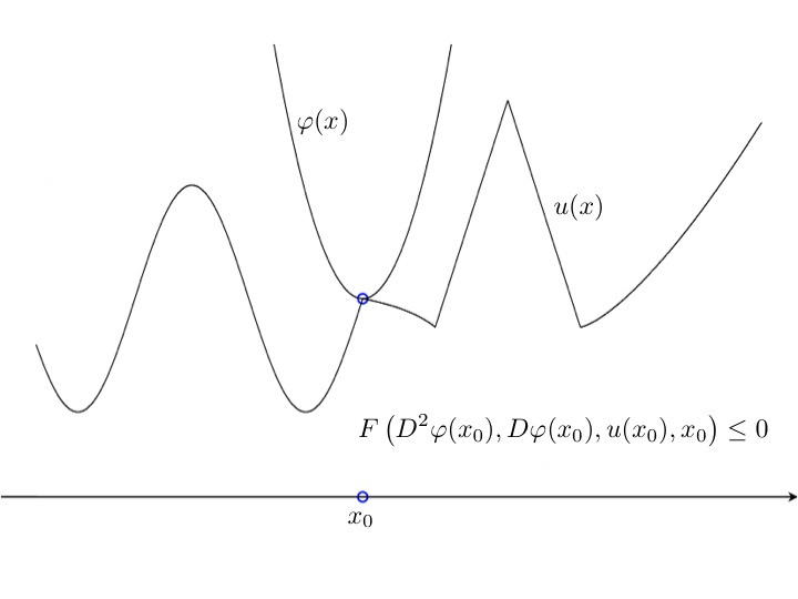
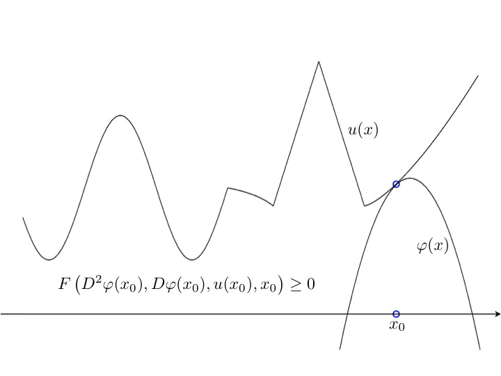
Fig. 1: A geometric interpretation of viscosity solutions for second order problems. The figure on the left corresponds to a viscosity subsolution being “touched” from above and the figure on the right corresponds to a viscosity supersolution being “touched” from below.

2.3 Ellipticity and the comparison principle

An advantage of the viscosity solution concept for fully nonlinear problems is that, due to its entirely local structure, it is flexible enough to seek solutions in the space of bounded functions. To ensure the existence and uniqueness of viscosity solutions, additional structure conditions on the differential operator $G$ are often necessary. The most common such conditions are an ellipticity requirement and a comparison principle. The following definitions of ellipticity and the comparison principle are standard (cf. [5]).

Definition 2.

(i) Equation (3) is said to be uniformly elliptic if, for all $(\mathbf{p},v,\mathbf{x})\in\mathbb{R}^{d}\times\mathbb{R}\times\overline{\Omega}$, there holds

$$\lambda\text{tr }(A-B)\leq G(B,\mathbf{p},v,\mathbf{x})-G(A,\mathbf{p},w,\mathbf{x})\leq\Lambda\text{tr }(A-B)$$

whenever $A\geq B$, where $A,B\in\mathcal{S}^{d\times d}$ and $A\geq B$ means that $A-B$ is a nonnegative definite matrix.

(ii) Equation (3) is said to be proper elliptic if, for all $(\mathbf{p},\mathbf{x})\in\mathbb{R}^{d}\times\overline{\Omega}$, there holds

$$G(A,\mathbf{p},v,\mathbf{x})\leq G(B,\mathbf{p},w,\mathbf{x})$$

whenever $v\leq w$ and $A\geq B$, where $v,w\in\mathbb{R}$ and $A,B\in\mathcal{S}^{d\times d}$.

(iii) Equation (3) is said to be degenerate elliptic if, for all $(\mathbf{p},v,\mathbf{x})\in\mathbb{R}^{d}\times\mathbb{R}\times\overline{\Omega}$, there holds

$$G(A,\mathbf{p},v,\mathbf{x})\leq G(B,\mathbf{p},v,\mathbf{x})$$

whenever $A\geq B$, where $A,B\in\mathcal{S}^{d\times d}$.

Definition 3.

Problem (3) is said to satisfy a comparison principle if the following statement holds. For any upper semicontinuous function $u$ and lower semicontinuous function $v$ on $\overline{\Omega}$, if $u$ is a viscosity subsolution and $v$ is a viscosity supersolution of (3), then $u\leq v$ on $\overline{\Omega}$.

The comparison principle is sometimes called a strong uniqueness property due to the fact it immediately yields the uniqueness of viscosity solutions for problem (3) (cf. [1]). When $G$ is differentiable, the degenerate ellipticity condition can also be defined by requiring that the matrix $\frac{\partial G}{\partial D^{2}u}$ is negative semi-definite while the proper ellipticity condition additionally requires the number $\frac{\partial G}{\partial u}$ is nonnegative (cf. [16, p. 441]). We then clearly see that the ellipticity concept for nonlinear problems generalizes the notion for linear elliptic equations.

Remark 2.2.

Since we have assumed that $G$ satisfies the comparison principle, it follows that that problem (3) has a unique viscosity solution $u\in C(\overline{\Omega})$.

2.4 Hamilton-Jacobi-Bellman equations

As mentioned in Section 1, a specific class of fully nonlinear PDEs that fits the structure requirements in this paper are (stationary) Hamilton-Jacobi-Bellman (HJB) equations described by (2).

We shall assume that $A^{\theta}$ is uniformly (in $\theta$) negative definite in the sense that there exists constants $0<\lambda\leq\Lambda$ such that

(5) $$-\Lambda|\xi|^{2}\leq A^{\theta}(\mathbf{x})\,\xi\cdot\xi\leq-\lambda|\xi|^{2}\qquad\forall\xi\in\mathbb{R}^{d},\mathbf{x}\in\Omega,\theta\in\Theta.$$

We also assume there exists a constant $K>0$ such that

$$\|A^{\theta}\|_{L^{\infty}(\Omega)},\,\|b^{\theta}\|_{L^{\infty}(\Omega)},\,\|c^{\theta}\|_{L^{\infty}(\Omega)}\leq K$$

and $c^{\theta}(\mathbf{x})\geq k_{0}>0$ for some constant $k_{0}$ for all $\mathbf{x}\in\Omega$ and $\theta\in\Theta$. Thus, the equation is proper elliptic and satisfies the comparison principle. We note that for stochastic optimal control applications, we have $c^{\theta}\equiv 0$ (cf. [15]). This case will also be considered. However, such problems may not satisfy a comparison principle as discussed in [24] and [28].

Under the above assumptions on the coefficients and the control set, problem (1)–(2) has a unique solution and $H$ is globally Lipschitz continuous. Thus, $H$ is differentiable almost everywhere and the weak derivatives are bounded by the constant $K$. Since $\Theta$ is closed and bounded, there actually exists a function $\theta^{*}(x)\in\Theta$ such that

$$H[u]=\min_{\theta\in\Theta}\bigl{(}L_{\theta}u-f_{\theta}\bigr{)}=A^{\theta^{*}}:D^{2}u+b^{\theta^{*}}\cdot\nabla u+c^{\theta^{*}}\,u=0\qquad\text{in }\Omega.$$

Thus, $\frac{\partial H}{\partial D^{2}u}=A^{\theta^{*}}$, $\frac{\partial H}{\partial\nabla u}=b^{\theta^{*}}$, and $\frac{\partial H}{\partial u}=c^{\theta^{*}}$, and we have $H$ is differentiable everywhere with bounded first order derivatives.

The analysis assumes a global Lipschitz condition for ease of presentation; however, locally Lipschitz should be sufficient. The global Lipschitz assumption excludes Monge-Ampère-type equations which are only conditionally degenerate elliptic [4] and locally Lipschitz. In light of the recent work [10], we know that the Monge-Ampère equation has an equivalent HJB reformulation. Much of the work of this paper can be extended to the Monge-Ampère equation via its HJB reformulation.

2.5 Difference operators

We introduce several difference operators for approximating first and second order partial derivatives. The multiple difference operators will be used to help resolve the low regularity of viscosity solutions and will play a key role in motivating and defining our new narrow-stencil FD methods.

Assume $\Omega$ is a $d$-rectangle, i.e., $\Omega=\left(a_{1},b_{1}\right)\times\left(a_{2},b_{2}\right)\times\cdots\times\left(a_{d},b_{d}\right)$. We shall only consider grids that are uniform in each coordinate $x_{i}$, $i=1,2,\ldots,d$. Let $J_{i}(\geq 2)$ be an integer and $h_{i}=\frac{b_{i}-a_{i}}{J_{i}-1}$ for $i=1,2,\ldots,d$. Define $\mathbf{h}=\left(h_{1},h_{2},\ldots,h_{d}\right)\in\mathbb{R}^{d}$, $h=\max_{i=1,2,\ldots,d}h_{i}$, $J=\prod_{i=1}^{d}J_{i}$, and $\mathbb{N}_{J}=\{\alpha=(\alpha_{1},\alpha_{2},\ldots,\alpha_{d})\mid 1\leq\alpha_{i}\leq J_{i},i=1,2,\ldots,d\}$. Then, $\left|\mathbb{N}_{J}\right|=J$. We partition $\Omega$ into $\prod_{i=1}^{d}\left(J_{i}-1\right)$ sub-$d$-rectangles with grid points $\mathbf{x}_{\alpha}=\bigl{(}a_{1}+(\alpha_{1}-1)h_{1},a_{2}+(\alpha_{2}-1)h_{2},\ldots,a_{d}+(\alpha_{d}-1)h_{d}\bigr{)}$ for each multi-index $\alpha\in\mathbb{N}_{J}$. We call $\mathcal{T}_{\mathbf{h}}=\{\mathbf{x}_{\alpha}\}_{\alpha\in\mathbb{N}_{J}}$ a mesh (set of nodes) for $\overline{\Omega}$. We also introduce an extended mesh $\mathcal{T}_{\mathbf{h}}^{\prime}$ which extends $\mathcal{T}_{\mathbf{h}}$ by a collection of ghost grid points that are at most one layer exterior to $\overline{\Omega}$ in each coordinate direction. In particular, we choose ghost grid points $\mathbf{x}$ such that $\mathbf{x}=\mathbf{y}\pm 2h_{i}\mathbf{e}_{i}$ for some $\mathbf{y}\in\mathcal{T}_{\mathbf{h}}\cap\Omega$, $i\in\{1,2,\ldots,d\}$. We set $J_{i}^{\prime}=J_{i}+2$ and $\mathbb{N}_{J}^{\prime}$ is defined by replacing $J_{i}$ by $J_{i}^{\prime}$ in the definition of $\mathbb{N}_{J}$ and then removing the extra multi-indices that would correspond to ghost grid points that are not in the set $\mathcal{T}_{\mathbf{h}}^{\prime}$ to ensure $|\mathbb{N}_{J}^{\prime}|=|\mathcal{T}_{\mathbf{h}}^{\prime}|$.

2.5.1 First order difference operators

We define the standard forward and backward difference operators as well as the central difference operator for approximating first order derivatives including the gradient operator. The forward and backward difference operators will serve as the building blocks for constructing all of the first and second order difference operators in this paper.

Let $\left\{\mathbf{e}_{i}\right\}_{i=1}^{d}$ denote the canonical basis vectors for $\mathbb{R}^{d}$. Define the (first order) forward and backward difference operators by

(6) $$\delta_{x_{i},h_{i}}^{+}v(\mathbf{x})\equiv\frac{v(\mathbf{x}+h_{i}\mathbf{e}_{i})-v(\mathbf{x})}{h_{i}},\qquad\delta_{x_{i},h_{i}}^{-}v(\mathbf{x})\equiv\frac{v(\mathbf{x})-v(\mathbf{x}-h_{i}\mathbf{e}_{i})}{h_{i}}$$

for a function $v$ defined on $\mathbb{R}^{d}$ and

$$\delta_{x_{i},h_{i}}^{+}V_{\alpha}\equiv\frac{V_{\alpha+\mathbf{e}_{i}}-V_{\alpha}}{h_{i}},\qquad\delta_{x_{i},h_{i}}^{-}V_{\alpha}\equiv\frac{V_{\alpha}-V_{\alpha-\mathbf{e}_{i}}}{h_{i}}$$

for a grid function $V$ defined on the grid $\mathcal{T}_{h}$. Note that “ghost-values” may need to be introduced in order for the above difference operators to be well-defined on the boundary of $\Omega$. We also define the following central difference operator:

(7) $$\delta_{x_{i},h_{i}}\equiv\frac{1}{2}\left(\delta_{x_{i},h_{i}}^{+}+\delta_{x_{i},h_{i}}^{-}\right)\qquad\mbox{for }i=1,2,\cdots,d.$$

Lastly, we define the “sided” and central gradient operators $\nabla_{\mathbf{h}}^{+}$, $\nabla_{\mathbf{h}}^{-}$, and $\nabla_{\mathbf{h}}$ by

(8) $$\nabla_{\mathbf{h}}^{\pm}\equiv\bigl{[}\delta^{\pm}_{x_{1},h_{1}},\delta_{x_{2},h_{2}}^{\pm},\cdots,\delta_{x_{d},h_{d}}^{\pm}\bigr{]}^{T},\quad\nabla_{\mathbf{h}}\equiv\bigl{[}\delta_{x_{1},h_{1}},\delta_{x_{2},h_{2}},\cdots,\delta_{x_{d},h_{d}}\bigr{]}^{T}.$$

2.5.2 Second order difference operators

We now introduce a number of difference operators that approximate second order derivatives including the Hessian operator. Using the forward and backward difference operators introduced in the previous subsection, we have the following four possible approximations of the second order differential operator $\partial^{2}_{x_{i}x_{j}}$:

$$D_{\mathbf{h},ij}^{\mu\nu}\equiv\delta_{x_{j},h_{j}}^{\nu}\delta_{x_{i},h_{i}}^{\mu}\qquad\mbox{for }\mu,\nu\in\{+,-\},$$

which in turn leads to the definition of the following four approximations of the Hessian operator $D^{2}\equiv[\partial^{2}_{x_{i}x_{j}}]$:

(9) $$D_{\mathbf{h}}^{\mu\nu}\equiv\bigl{[}D_{\mathbf{h},ij}^{\mu\nu}\bigr{]}_{i,j=1}^{d}\qquad\mbox{for }\mu,\nu\in\{+,-\}.$$

To construct our numerical methods in the next section, we also need to introduce the following three sets of averaged second order difference operators:

(10a) $$\widehat{\delta}_{x_{i},x_{j};h_{i},h_{j}}^{2} \equiv\frac{1}{2}\bigl{(}D_{\mathbf{h},ij}^{+-}+D_{\mathbf{h},ij}^{-+}\bigr{)}=\frac{1}{2}\bigl{(}\delta_{x_{j},h_{j}}^{-}\delta_{x_{i},h_{i}}^{+}+\delta_{x_{j},h_{j}}^{+}\delta_{x_{i},h_{i}}^{-}\bigr{)},$$

(10b) $$\widetilde{\delta}_{x_{i},x_{j};h_{i},h_{j}}^{2} \equiv\frac{1}{2}\bigl{(}D_{\mathbf{h},ij}^{--}+D_{\mathbf{h},ij}^{++}\bigr{)}=\frac{1}{2}\bigl{(}\delta_{x_{j},h_{j}}^{+}\delta_{x_{i},h_{i}}^{+}+\delta_{x_{j},h_{j}}^{-}\delta_{x_{i},h_{i}}^{-}\bigr{)},$$

(10c) $$\overline{\delta}_{x_{i},x_{j};h_{i},h_{j}}^{2} \equiv\frac{1}{2}\bigl{(}\widehat{\delta}_{x_{i},x_{j};h_{i},h_{j}}^{2}+\widetilde{\delta}_{x_{i},x_{j};h_{i},h_{j}}^{2}\bigr{)}=\frac{1}{4}\bigl{(}D_{\mathbf{h},ij}^{++}+D_{\mathbf{h},ij}^{+-}+D_{\mathbf{h},ij}^{-+}+D_{\mathbf{h},ij}^{--}\bigr{)}$$

$$=\frac{1}{4}\left(\delta_{x_{j},h_{j}}^{+}\delta_{x_{i},h_{i}}^{+}+\delta_{x_{j},h_{j}}^{-}\delta_{x_{i},h_{i}}^{+}+\delta_{x_{j},h_{j}}^{+}\delta_{x_{i},h_{i}}^{-}+\delta_{x_{j},h_{j}}^{-}\delta_{x_{i},h_{i}}^{-}\right)$$

for all $i,j=1,2,\ldots,d$. For notation brievity, we also set

$$\delta_{x_{i},h_{i}}^{2}\equiv\widehat{\delta}_{x_{i},h_{i}}^{2}\equiv\widehat{\delta}_{x_{i},x_{i};h_{i},h_{i}}^{2},\qquad\widetilde{\delta}_{x_{i},h_{i}}^{2}\equiv\widetilde{\delta}_{x_{i},x_{i};h_{i},h_{i}}^{2},\qquad\overline{\delta}_{x_{i},h_{i}}^{2}\equiv\overline{\delta}_{x_{i},x_{i};h_{i},h_{i}}^{2}.$$

Using the above difference operators, we define the following three “centered” approximations of the Hessian operator $D^{2}\equiv[\partial^{2}_{x_{i}x_{j}}]$:

(11) $$\widehat{D}_{\mathbf{h}}^{2}=\bigl{[}\widehat{\delta}_{x_{i},x_{j};h_{i},h_{j}}^{2}\bigr{]}_{i,j=1}^{d},\quad\widetilde{D}_{\mathbf{h}}^{2}=\bigl{[}\widetilde{\delta}_{x_{i},x_{j};h_{i},h_{j}}^{2}\bigr{]}_{i,j=1}^{d},\quad\overline{D}_{\mathbf{h}}^{2}=\bigl{[}\overline{\delta}_{x_{i},x_{j};h_{i},h_{j}}^{2}\bigr{]}_{i,j=1}^{d}.$$

We will also consider the (standard) central approximation of the Hessian operator $D_{\mathbf{h}}^{2}$ defined by

(12) $$\left[D_{\mathbf{h}}^{2}\right]_{ij}\equiv\begin{cases}\delta_{x_{i},h_{i}}^{2}&\text{if }i=j,\\ \overline{\delta}_{x_{i},x_{j};h_{i},h_{j}}^{2},\qquad&\text{if }i\neq j.\end{cases}$$

We now record some facts that can be easily verified for the various second order operators. First,

$$2\widehat{D}_{\mathbf{h}}^{2}=D_{\mathbf{h}}^{+-}+D_{\mathbf{h}}^{-+},\quad 2\widetilde{D}_{\mathbf{h}}^{2}=D_{\mathbf{h}}^{--}+D_{\mathbf{h}}^{++},\quad 2\overline{D}_{\mathbf{h}}^{2}=\widehat{D}_{\mathbf{h}}^{2}+\widetilde{D}_{\mathbf{h}}^{2}.$$

Second, a simple computation reveals

(13a) $$\widehat{\delta}_{x_{i},x_{j};h_{i},h_{j}}^{2}v(\mathbf{x}) =-\frac{v(\mathbf{x}+h_{i}\mathbf{e}_{i}-h_{j}\mathbf{e}_{j})-v(\mathbf{x}+h_{i}\mathbf{e}_{i})-\big{[}v(\mathbf{x}-h_{j}\mathbf{e}_{j})-v(\mathbf{x})\big{]}}{2h_{i}h_{j}}$$

$$\quad-\frac{v(\mathbf{x}-h_{i}\mathbf{e}_{i}+h_{j}\mathbf{e}_{j})-v(\mathbf{x}-h_{i}\mathbf{e}_{i})-\big{[}v(\mathbf{x}+h_{j}\mathbf{e}_{j})-v(\mathbf{x})\big{]}}{2h_{i}h_{j}},$$

(13b) $$\widetilde{\delta}_{x_{i},x_{j};h_{i},h_{j}}^{2}v(\mathbf{x}) =\frac{v(\mathbf{x}+h_{i}\mathbf{e}_{i}+h_{j}\mathbf{e}_{j})-v(\mathbf{x}+h_{i}\mathbf{e}_{i})-\big{[}v(\mathbf{x}+h_{j}\mathbf{e}_{j})-v(\mathbf{x})\big{]}}{2h_{i}h_{j}}$$

$$\quad+\frac{v(\mathbf{x}-h_{i}\mathbf{e}_{i}-h_{j}\mathbf{e}_{j})-v(\mathbf{x}-h_{i}\mathbf{e}_{i})-\big{[}v(\mathbf{x}-h_{j}\mathbf{e}_{j})-v(\mathbf{x})\big{]}}{2h_{i}h_{j}},$$

(13c) $$\overline{\delta}_{x_{i},x_{j};h_{i},h_{j}}^{2}v(\mathbf{x}) =\frac{v(\mathbf{x}+h_{i}\mathbf{e}_{i}+h_{j}\mathbf{e}_{j})+v(\mathbf{x}-h_{i}\mathbf{e}_{i}-h_{j}\mathbf{e}_{j})}{4h_{i}h_{j}}$$

$$\quad-\frac{v(\mathbf{x}-h_{i}\mathbf{e}_{i}+h_{j}\mathbf{e}_{j})+v(\mathbf{x}+h_{i}\mathbf{e}_{i}-h_{j}\mathbf{e}_{j})}{4h_{i}h_{j}}.$$

Lastly, there holds the relationships

(14a) $$\delta_{x_{i},h_{i}}^{2} =\delta_{x_{i},h_{i}}^{\pm}\delta_{x_{i},h_{i}}^{\mp},$$

(14b) $$\delta_{x_{i},2h_{i}}^{2} =\overline{\delta}_{x_{i},h_{i}}^{2}=\delta_{x_{i},h_{i}}\delta_{x_{i},h_{i}}.$$

We have $\delta_{x_{i},h_{i}}^{2}\equiv\widehat{\delta}_{x_{i},h_{i}}^{2}$ is the standard (second order) three-point central difference operator for approximating second order derivatives in one-dimension, $\overline{\delta}_{x_{i},h_{i}}^{2}=\delta_{x_{i},2h_{i}}^{2}$ is a lower-resolution (second-order) three-point central difference operator for approximating second order derivatives in one-dimension, $\widetilde{\delta}_{x_{i},h_{i}}^{2}$ is a (second order) five-point central difference operator for approximating second order derivatives in one-dimension, $\overline{\delta}_{x_{i},x_{j};h_{i},h_{j}}^{2}$ is the standard (second order) central difference operator for approximating second order mixed derivatives, and $\widehat{\delta}_{x_{i},x_{j};h_{i},h_{j}}^{2}$ and $\widetilde{\delta}_{x_{i},x_{j};h_{i},h_{j}}^{2}$ are two alternative (second order) central difference operators for approximating second order mixed derivatives. Observe that in two dimensions, $\widehat{D}_{\mathbf{h}}^{2}$ corresponds to a 7-point stencil, $\overline{D}_{\mathbf{h}}^{2}$ and $D_{\mathbf{h}}^{2}$ correspond to 9-point stencils, and $\widetilde{D}_{\mathbf{h}}^{2}$ corresponds to an 11-point stencil, as seen in Figure 2. The operators $\widehat{D}_{\mathbf{h}}^{2}$ and $D_{\mathbf{h}}^{2}$ use nearest neighbors in the stencil (including diagonal directions) while $\overline{D}_{\mathbf{h}}^{2}$ and $\widetilde{D}_{\mathbf{h}}^{2}$ use neighbors two steps away in each Cartesian direction.

Fig. 2: Local stencils for the discrete central Hessian operators $\widehat{D}_{\mathbf{h}}^{2}v$, $\widetilde{D}_{\mathbf{h}}^{2}v$, $\overline{D}_{\mathbf{h}}^{2}v$, and $D_{\mathbf{h}}^{2}v$ in two dimensions. Circled nodes correspond to a discrete approximation of $v_{xx}$. Boxed nodes correspond to a discrete approximation of $v_{xy}$. Nodes with a diamond correspond to a discrete approximation of $v_{yy}$.

We lastly introduce the (diagonal) variables $\xi_{i}^{j}=\xi_{j}^{i}$ and $\eta_{i}^{j}=\eta_{j}^{i}$ so that we can define the central difference operators $\delta_{\xi_{i}^{j},\mathbf{h}}^{2}$ and $\delta_{\eta_{i}^{j},\mathbf{h}}^{2}$ by

(15a) $$\delta_{\xi_{i}^{j},\mathbf{h}}^{2}v(\mathbf{x}) \equiv\frac{v(\mathbf{x}-h_{i}\mathbf{e}_{i}+h_{j}\mathbf{e}_{j})-2v(\mathbf{x})+v(\mathbf{x}+h_{i}\mathbf{e}_{i}-h_{j}\mathbf{e}_{j})}{h_{i}^{2}+h_{j}^{2}},$$

(15b) $$\delta_{\eta_{i}^{j},\mathbf{h}}^{2}v(\mathbf{x}) \equiv\frac{v(\mathbf{x}+h_{i}\mathbf{e}_{i}+h_{j}\mathbf{e}_{j})-2v(\mathbf{x})+v(\mathbf{x}-h_{i}\mathbf{e}_{i}-h_{j}\mathbf{e}_{j})}{h_{i}^{2}+h_{j}^{2}}$$

for all $i,j=1,2,\ldots,d$ with $i\neq j$. Then, a direct computation yields

(16a) $$\bigl{[}\overline{D}_{\mathbf{h}}^{2}v\bigr{]}_{ij} =\bigl{[}D_{\mathbf{h}}^{2}v\bigr{]}_{ij}=\frac{h_{i}^{2}+h_{j}^{2}}{4h_{i}h_{j}}\left(\delta_{\eta_{i}^{j},\mathbf{h}}^{2}v-\delta_{\xi_{i}^{j},\mathbf{h}}^{2}v\right),$$

(16b) $$\bigl{[}\widehat{D}_{\mathbf{h}}^{2}v\bigr{]}_{ij} =\frac{h_{i}}{2h_{j}}\delta_{x_{i},h_{i}}^{2}v+\frac{h_{j}}{2h_{i}}\delta_{x_{j},h_{j}}^{2}v-\frac{h_{i}^{2}+h_{j}^{2}}{2h_{i}h_{j}}\delta_{\xi_{i}^{j},\mathbf{h}}^{2}v,$$

(16c) $$\bigl{[}\widetilde{D}_{\mathbf{h}}^{2}v\bigr{]}_{ij} =-\frac{h_{i}}{2h_{j}}\delta_{x_{i},h_{i}}^{2}v-\frac{h_{j}}{2h_{i}}\delta_{x_{j},h_{j}}^{2}v+\frac{h_{i}^{2}+h_{j}^{2}}{2h_{i}h_{j}}\delta_{\eta_{i}^{j},\mathbf{h}}^{2}v,$$

relationships that are illustrated in Figure 3. Lastly, there holds

(17) $$\bigl{[}\widetilde{D}_{\mathbf{h}}^{2}V_{\alpha}\bigr{]}_{ii}-\bigl{[}\widehat{D}_{\mathbf{h}}^{2}V_{\alpha}\bigr{]}_{ii} =\widetilde{\delta}_{x_{i},h_{i}}^{2}V_{\alpha}-\delta_{x_{i},h_{i}}^{2}V_{\alpha}$$

$$=2\left(\delta_{x_{i},2h_{i}}^{2}V_{\alpha}-\delta_{x_{i},h_{i}}^{2}V_{\alpha}\right)$$

$$=\frac{1}{2}\left(\delta_{x_{i},h_{i}}^{2}V_{\alpha-\mathbf{e}_{i}}-2\delta_{x_{i},h_{i}}^{2}V_{\alpha}+\delta_{x_{i},h_{i}}^{2}V_{\alpha+\mathbf{e}_{i}}\right)$$

for all $i=1,2,\ldots,d$.

Fig. 3: Illustration of the relationship between the Cartesian directions and diagonal directions when defining various mixed second order partial derivative approximations. Blue corresponds to added three-point (non-mixed) second derivative approximations and red corresponds to subtracted three-point (non-mixed) second derivative approximations.

3 A narrow-stencil finite difference method

We now propose a new finite difference method for approximating viscosity solutions of the fully nonlinear second order problem (1). In the construction of such a narrow-stencil scheme, our main idea is to design a numerical operator that utilizes the various numerical Hessians defined in the previous section so that a relaxed (or generalized) monotonicity condition is satisfied. The crux of the formulation is to introduce the concept of numerical moments which can be considered analogous to the concept of numerical viscosities used in the Crandall and Lions’ finite difference framework for (first order) Hamilton-Jacobi equations. Below, we first define our narrow-stencil finite difference method, and we then describe the idea and details of numerical moments. We also prove a generalized monotonicity result for our proposed numerical operator.

3.1 Formulation of the narrow-stencil finite difference method

In Section 2.5.2 we defined four basic sided discrete Hessian operators $D_{\mathbf{h}}^{\mu\nu}$ for $\mu,\nu\in\{+,-\}$. These four operators are the building blocks for constructing our numerical operator $\widehat{F}$ that approximates the differential operator $F$. However, inspired by our earlier 1-D work [14], we construct the numerical operator $\widehat{F}$ so that it only depends explicitly upon the central difference operators $\widehat{D}_{\mathbf{h}}^{2}$ and $\widetilde{D}_{\mathbf{h}}^{2}$ with regard to the Hessian argument in $F$. Recall that $\mathcal{T}_{\mathbf{h}}^{\prime}$ denotes the extended mesh of $\overline{\Omega}$ that includes ghost mesh points and $\mathbb{N}_{J}^{\prime}$ is the corresponding extended index set of $\mathbb{N}_{J}$ (see Section 2.5).

Our specific narrow-stencil finite difference method is defined by seeking a grid function $U_{\alpha}:\mathbb{N}_{J}^{\prime}\to\mathbb{R}$ such that for all $\alpha\in\mathbb{N}_{J}$

(18a) $$\widehat{F}[U_{\alpha},\mathbf{x}_{\alpha}] =0 \qquad\mbox{for }\mathbf{x}_{\alpha}\in\mathcal{T}_{\mathbf{h}}\cap\Omega,$$

(18b) $$U_{\alpha} =g(\mathbf{x}_{\alpha}) \qquad\mbox{for }\mathbf{x}_{\alpha}\in\mathcal{T}_{\mathbf{h}}\cap\partial\Omega,$$

where

(19) $$\widehat{F}[U_{\alpha},\mathbf{x}_{\alpha}] \equiv\widetilde{F}\bigl{(}D_{\mathbf{h}}^{--}U_{\alpha},D_{\mathbf{h}}^{-+}U_{\alpha},D_{\mathbf{h}}^{+-}U_{\alpha},D_{\mathbf{h}}^{++}U_{\alpha},\nabla_{\mathbf{h}}^{+}U_{\alpha},\nabla_{\mathbf{h}}^{-}U_{\alpha},U_{\alpha},\mathbf{x}_{\alpha}\bigr{)}$$

$$\equiv\widehat{F}(\widehat{D}_{\mathbf{h}}^{2}U_{\alpha},\widetilde{D}_{\mathbf{h}}^{2}U_{\alpha},\nabla_{\mathbf{h}}^{+}U_{\alpha},\nabla_{\mathbf{h}}^{-}U_{\alpha},U_{\alpha},\mathbf{x}_{\alpha})$$

$$\equiv F\left(\overline{D}_{\mathbf{h}}^{2}U_{\alpha},\nabla_{\mathbf{h}}U_{\alpha},U_{\alpha},\mathbf{x}_{\alpha}\right)+A(U_{\alpha},\mathbf{x}_{\alpha}):\bigl{(}\widetilde{D}_{\mathbf{h}}^{2}U_{\alpha}-\widehat{D}_{\mathbf{h}}^{2}U_{\alpha}\bigr{)}$$

$$\qquad-\vec{\beta}(U_{\alpha},\mathbf{x}_{\alpha})\cdot\bigl{(}\nabla_{\mathbf{h}}^{+}U_{\alpha}-\nabla_{\mathbf{h}}^{-}U_{\alpha}\bigr{)},$$

for $A:\mathbb{R}^{J}\times\mathcal{T}_{\mathbf{h}}\to\mathbb{R}^{d\times d}$ a matrix-valued function and $\vec{\beta}:\mathbb{R}^{J}\times\mathcal{T}_{\mathbf{h}}\to\mathbb{R}^{d}$ a vector-valued function. Recall that $2\overline{D}_{\mathbf{h}}^{2}U_{\alpha}=\widetilde{D}_{\mathbf{h}}^{2}U_{\alpha}+\widehat{D}_{\mathbf{h}}^{2}U_{\alpha}$ and $2\nabla_{\mathbf{h}}U_{\alpha}=\nabla_{\mathbf{h}}^{+}U_{\alpha}+\nabla_{\mathbf{h}}^{-}U_{\alpha}$. Hence, $\overline{D}_{\mathbf{h}}^{2}U_{\alpha}$ and $\nabla_{\mathbf{h}}U_{\alpha}$ are not regarded as independent variables in the function $\widehat{F}$. We also note that the explicit dependence of $\widehat{F}$ on the $U_{\alpha}$ and $\mathbf{x}_{\alpha}$ arguments is inherited from $F$. Suitable choices for $A$ and $\vec{\beta}$ will be specified in Section 3.3 to guarantee well-posedness and convergence of the scheme.

In order for the above scheme to be well defined, the issue of how to provide the ghost values must be addressed. This is because when $\mathbf{x}_{\alpha}$ is next to the boundary $\partial\Omega$, equation (18a) uses ghost grid points which are outside of the domain $\Omega$ when evaluating $\widetilde{D}_{\mathbf{h}}^{2}U_{\alpha}$. Inspired by our 1-D work [14], we propose to use the following auxiliary equations, which can be viewed as a discretization of an additional boundary condition, to define the required ghost values in terms of the boundary and interior grid values:

(20) $$\Delta_{\mathbf{h}}U_{\alpha}\equiv\sum_{i=1}^{d}\delta_{x_{i},h_{i}}^{2}U_{\alpha}=0\qquad\mbox{for }\mathbf{x}_{\alpha}\in\mathcal{S}_{\mathbf{h}}\subset\mathcal{T}_{\mathbf{h}}\cap\partial\Omega,$$

where

(21) $$\mathcal{S}_{\mathbf{h}}\equiv\big{\{}\mathbf{x}_{\alpha}\in\mathcal{T}_{\mathbf{h}}\cap\partial\Omega\mid \,\mathbf{x}_{\alpha}+h_{i}\mathbf{e}_{i}\in\mathcal{T}_{\mathbf{h}}\cap\Omega\text{ or }\mathbf{x}_{\alpha}-h_{i}\mathbf{e}_{i}\in\mathcal{T}_{\mathbf{h}}\cap\Omega$$

$$\text{ for some }i\in\{1,2,\ldots,d\}\big{\}}.$$

We refer the reader to [14, 21, 12] for detailed explanations of why such auxiliary equations are appropriate from the PDE point of view. See Figure 4 for an illustration of how to implement the auxiliary boundary condition (20).

We remark that the definition of scheme (18)–(20) does not depend on the particular structure of the differential operator $F$. Hence, it is defined for all fully nonlinear second order PDEs including HJB equations and Monge-Ampère-type equations. We also note that the numerical operator $\widehat{F}$ defined by (19) satisfies a consistency property which says that $\widehat{F}[U_{\alpha},\mathbf{x}_{\alpha}]=F(P,\mathbf{q},U_{\alpha},\mathbf{x}_{\alpha})$ provided $\widetilde{D}_{\mathbf{h}}^{2}U_{\alpha}=\widehat{D}_{\mathbf{h}}^{2}U_{\alpha}=P$ and $\nabla_{\mathbf{h}}^{+}U_{\alpha}=\nabla_{\mathbf{h}}^{-}U_{\alpha}=\mathbf{q}$.

Fig. 4: An example in two dimensions of how to enforce the auxiliary boundary condition when building the matrix representation of $\delta_{x_{i},2h_{i}}^{2}$. The circled nodes correspond to evaluating $\Delta_{2\mathbf{h}}U_{1}$. The blue and red ghost nodes are defined using the auxiliary boundary condition $\Delta_{\mathbf{h}}U_{\alpha}=0$ along $\partial\Omega$. The blue and red nodes along $\partial\Omega$ are treated as knowns. Thus, we can replace the ghost nodes with unknown nodes corresponding to grid points in the interior of the domain as well as known values coming from the Dirichlet boundary condition. Note that the green nodes are ghost nodes that are not needed since they do not appear in the calculation of $\widehat{F}[U]$. Accordingly, the corner mesh node is not included in the construction of the set $\mathcal{S}_{\mathbf{h}}$ over which the auxiliary boundary condition is enforced.

3.2 Numerical moments

Since the last two terms in (19) where the numerical operator $\widehat{F}$ is defined are special, we now take a closer look at them and explain the insights behind their introduction. First, a direct calculation immediately yields

(22) $$\delta_{x_{i},h_{i}}^{+}U_{\alpha}-\delta_{x_{i},h_{i}}^{-}U_{\alpha}=h_{i}\,\frac{U_{\alpha-h_{i}\mathbf{e}_{i}}-2U_{\alpha}+U_{\alpha+h_{i}\mathbf{e}_{i}}}{h_{i}^{2}}=h_{i}\,\delta_{x_{i},h_{i}}^{2}U_{\alpha},$$

which is a central difference approximation of $u_{x_{i}x_{i}}(\mathbf{x}_{\alpha})$ scaled by $h_{i}$. This is the very reason that this term is called a numerical viscosity in the literature, and it was used in [7] to construct a Lax-Friedrichs monotone scheme for Hamilton-Jacobi equations.

Second, also by a direct calculation, we get for $i,j\in\{1,2,\ldots,d\}$

(23) $$\bigl{[}\widetilde{D}_{\mathbf{h}}^{2}V_{\alpha}\bigr{]}_{ij}-\bigl{[}\widehat{D}_{\mathbf{h}}^{2}V_{\alpha}\bigr{]}_{ij} =\frac{1}{2}\bigl{(}\delta_{x_{i},h_{i}}^{+}\delta_{x_{j},h_{j}}^{+}-\delta_{x_{i},h_{i}}^{+}\delta_{x_{j},h_{j}}^{-}-\delta_{x_{i},h_{i}}^{-}\delta_{x_{j},h_{j}}^{+}+\delta_{x_{i},h_{i}}^{-}\delta_{x_{j},h_{j}}^{-}\bigr{)}V_{\alpha}$$

$$=\frac{h_{i}h_{j}}{2}\delta_{x_{i},h_{i}}^{2}\delta_{x_{j},h_{j}}^{2}V_{\alpha}=\frac{h_{i}h_{j}}{2}\delta_{x_{j},h_{j}}^{2}\delta_{x_{i},h_{i}}^{2}V_{\alpha},$$

which is an $O(h_{i}^{2}+h_{j}^{2})$ approximation of $v_{x_{i}x_{i}x_{j}x_{j}}(\mathbf{x}_{\alpha})$ scaled by $h_{i}h_{j}/2$. Thus,

$$2\mathbf{1}_{d\times d}:\left(\widetilde{D}_{\mathbf{h}}^{2}-\widehat{D}_{\mathbf{h}}^{2}\right)V_{\alpha}\approx h^{2}\Delta^{2}v(\mathbf{x}_{\alpha}),$$

where $\mathbf{1}_{d\times d}$ denotes the $d\times d$ matrix with all entries equal to $1$.

Due to the above observation and motivated by its connection to the vanishing moment method of [11], we introduce the following definition for the above expression.

Definition 4.

Let $A:\mathbb{R}^{J}\times\mathcal{T}_{\mathbf{h}}\to\mathbb{R}^{d\times d}$ and $V$ be a given grid function. The discrete operator $M:\mathbb{R}^{J}\to\mathbb{R}$ defined by

$$M[V,\mathbf{x}_{\alpha}]\equiv A\bigl{(}V_{\alpha},\mathbf{x}_{\alpha}\bigr{)}:\bigl{(}\widetilde{D}_{\mathbf{h}}^{2}V_{\alpha}-\widehat{D}_{\mathbf{h}}^{2}V_{\alpha}\bigr{)}$$

for all $\mathbf{x}_{\alpha}\in\mathcal{T}_{\mathbf{h}}\cap\Omega$ is called a numerical moment operator.

Let $M_{ij}$ denote the $(i,j)$ component of the matrix difference $\bigl{[}\widetilde{D}_{\mathbf{h}}^{2}V_{\alpha}\bigr{]}-\bigl{[}\widehat{D}_{\mathbf{h}}^{2}V_{\alpha}\bigr{]}$ and let $A_{i}$ and $A_{j}$ denote the matrix representations of the difference quotients $-\delta_{x_{i},h_{i}}^{2}V_{\alpha}$ and $-\delta_{x_{j},h_{j}}^{2}V_{\alpha}$ with Dirichlet boundary conditions, respectively. Then,

$$M_{ij}=\frac{1}{2}h_{i}h_{j}A_{i}A_{j}=\frac{1}{2}h_{i}h_{j}A_{j}A_{i}.$$

Since $A_{i}$ and $A_{j}$ are symmetric positive definite, it follows that $M_{ij}$ is symmetric positive definite. Thus, the numerical moment is a strictly positive operator. Similarly, by (22), we have the numerical viscosity is also a strictly positive operator.

3.3 Generalized monotonicity properties of the numerical operator $\widehat{F}$

In the definition of $\widehat{F}$, no restriction or guideline is given for the choices of the matrix-valued function $A$ and the vector-valued function $\vec{\beta}$. Suggested by the admissibility and stability proofs to be given in subsequent sections, we consider a special family of the pairs $A$ and $\vec{\beta}$, that is, $A=\gamma\mathbf{1}_{d\times d}$ for some constant $\gamma>0$ and $\vec{\beta}=\beta\vec{1}$ for some constant $\beta\geq 0$, where $\mathbf{1}_{d\times d}$ and $\vec{1}$ denote the matrix and the vector with all entries equal to one, respectively. Thus, the numerical operator is a linear perturbation of the nonlinear operator $F$. We note that the particular choice for $\gamma$ and $\beta$ depends on the Lipschitz constants of the differential operator $F$ which we now explain. For the ease of presentation we only present the details for the case that $F$ is differentiable with respect to its first three arguments and make a comment for the Lipschitz continuous case at the end.

Since $F$ is proper elliptic and differentiable, there exist constants $K_{ii}\geq k_{ii}>0$, $k_{0}\geq 0$, and $K_{ij},K_{i},K^{0}\geq 0$ such that

$$-K_{ii}\leq\frac{\partial F}{\partial u_{x_{i}x_{i}}}\leq-k_{ii},\qquad k_{0}\leq\frac{\partial F}{\partial u}\leq K^{0},$$

$$\left|\frac{\partial F}{\partial u_{x_{i}x_{j}}}\right|\leq K_{ij},\qquad \left|\frac{\partial F}{\partial u_{x_{i}}}\right|\leq K_{i}$$

for all $i,j$. Let $k_{**}=\min\{k_{ii}\}$, $K^{**}=\max\left\{K_{ij}\right\}$, and $K^{*}=\max\left\{K_{i}\right\}$.

By the definition of $\overline{D}_{\mathbf{h}}^{2}U_{\alpha}$ and $\nabla_{\mathbf{h}}U_{\alpha}$, we get

(24a) $$\frac{\partial\widehat{F}}{\partial\widetilde{D}_{\mathbf{h}}^{2}U_{\alpha}} =\frac{1}{2}\frac{\partial F}{D^{2}u}+\gamma\mathbf{1}_{d\times d}\geq\left(\gamma-\frac{1}{2}K^{**}\right)\mathbf{1}_{d\times d},$$

(24b) $$\frac{\partial\widehat{F}}{\partial\widehat{D}_{\mathbf{h}}^{2}U_{\alpha}} =\frac{1}{2}\frac{\partial F}{D^{2}u}-\gamma\mathbf{1}_{d\times d}\leq\left(\frac{1}{2}K^{**}-\gamma\right)\mathbf{1}_{d\times d},$$

(24c) $$\frac{\partial\widehat{F}}{\partial\nabla_{\mathbf{h}}^{+}U_{\alpha}} =\frac{1}{2}\frac{\partial F}{\partial\nabla u}-\beta\vec{1}\leq\left(\frac{1}{2}K^{*}-\beta\right)\vec{1},$$

(24d) $$\frac{\partial\widehat{F}}{\partial\nabla_{\mathbf{h}}^{-}U_{\alpha}} =\frac{1}{2}\frac{\partial F}{\partial\nabla u}+\beta\vec{1}\geq\left(\beta-\frac{1}{2}K^{*}\right)\vec{1},$$

(24e) $$\frac{\partial\widehat{F}}{\partial U_{\alpha}} =\frac{\partial F}{\partial u}\geq k_{0},$$

where the inequalities hold component-wise. Clearly, for sufficiently large $\gamma$ and $\beta$, every partial derivative in (24) has a fixed sign as reflected in the following lemma.

Lemma 5.

Assume that $F$ is proper elliptic and has bounded derivatives with respect to its first three arguments for all $x\in\Omega$. Then for sufficiently large $\gamma>0$ and $\beta\geq 0$, the numerical operator $\widehat{F}$ is nonincreasing with respect to each component of $\widehat{D}_{\mathbf{h}}^{2}U_{\alpha}$ and $\nabla_{\mathbf{h}}^{+}U_{\alpha}$ and nondecreasing with respect to each component of $\widetilde{D}_{\mathbf{h}}^{2}U_{\alpha}$, $\nabla_{\mathbf{h}}^{-}U_{\alpha}$, and $U_{\alpha}$.

Proof.

The assertion holds by (24) if $\gamma$ and $\beta$ are chosen such that $\gamma\geq\frac{K^{**}}{2}$ and $\beta\geq\frac{K^{*}}{2}$. The proof is complete. ∎

Remark 3.1.

(a) It is easy to see that the conclusion of Lemma 5 still holds if $F$ is proper elliptic and Lipschitz continuous with respect to its first three arguments for all $x\in\Omega$. This is because the inequalities in (24) still hold if all of the partial derivatives are replaced by their respective difference quotients, which is sufficient to ensure the monotonicity stated in the lemma.

(b) It should be noted that the monotonicity proved above in Lemma 5 is nonstandard. First, it holds only with respect to the various zero-, first-, and second-order difference operators. Second, the monotonicity with respect to each matrix or vector argument holds component-wise; in other words, in a component-wise ordering for these matrix or vector arguments.

(c) We shall refer to the monotonicity stated in Lemma 5 for $\widehat{F}$ as generalized monotonicity conditions throughout the rest of the paper. We also note that, for $h$ sufficiently small, we can choose $\beta=0$ when $k_{**}>0$. i.e., $F$ is not degenerate elliptic.

4 $\ell^{2}$-norm stability and well-posedness

The goal of this section is to show that the proposed narrow stencil scheme as defined in Section 3.3 with the choices of the parameters

(25) $$A=\gamma\mathbf{1}_{d\times d},\qquad\vec{\beta}=\beta\vec{1}$$

has a unique solution for sufficiently large $\gamma,\beta\geq 0$ that is uniformly bounded in a weighted $\ell^{2}$ norm. For transparency, we consider the second-order PDE problem

(26a) $$F[u](\mathbf{x})\equiv F\left(D^{2}u,u,\mathbf{x}\right) =0 \qquad\forall\mathbf{x}\in\Omega\subset\mathbb{R}^{d},$$

(26b) $$u(\mathbf{x}) =g(\mathbf{x}) \qquad\forall\mathbf{x}\in\partial\Omega.$$

We assume that $F$ is degenerate elliptic (see Definition 2), differentiable, and Lipschitz with respect to the first two arguments. Since $F$ is independent of $\nabla u$ in (26), we choose $\beta=0$. We note that the results for this special case can be extended to the more general PDE (1).

The idea for proving the well-posedness and stability of the method is to equivalently reformulate the proposed scheme as a fixed point problem for a nonlinear mapping and to prove the mapping is contractive in the $\ell^{2}$-norm. The well-posedness of the scheme then follows from the Contractive Mapping Theorem and the weighted $\ell^{2}$-norm stability will be obtained as a consequence of the contractive property. To this end, let $S(\mathcal{T}_{\mathbf{h}}^{\prime})$ denote the space of all grid functions on $\mathcal{T}_{\mathbf{h}}^{\prime}$, and introduce the mapping $\mathcal{M}_{\rho}:S(\mathcal{T}_{\mathbf{h}}^{\prime})\to S(\mathcal{T}_{\mathbf{h}}^{\prime})$ defined by

(27) $$\widehat{U}\equiv\mathcal{M}_{\rho}U,$$

where the grid function $\widehat{U}\in S(\mathcal{T}_{\mathbf{h}}^{\prime})$ is defined by

(28a) $$\widehat{U}_{\alpha} =U_{\alpha}-\rho\widehat{F}\left[U_{\alpha},\mathbf{x}_{\alpha}\right],\qquad \text{if }\mathbf{x}_{\alpha}\in\mathcal{T}_{\mathbf{h}}\cap\Omega,$$

(28b) $$\widehat{U}_{\alpha} =g(\mathbf{x}_{\alpha}), \text{if }\mathbf{x}_{\alpha}\in\mathcal{T}_{\mathbf{h}}\cap\partial\Omega,$$

(28c) $$\Delta_{\mathbf{h}}\widehat{U}_{\alpha} =0, \text{if }\mathbf{x}_{\alpha}\in\mathcal{S}_{\mathbf{h}}\subset\mathcal{T}_{\mathbf{h}}\cap\partial\Omega$$

for $\rho>0$ an underdetermined constant. Clearly, the iteration defined in (28) is the standard forward Euler method with pseudo time-step $\rho$. In the following, we will show that the mapping $\mathcal{M}_{\rho}$ is a contraction with respect to the $\ell^{2}$ norm when $\gamma>0$ is sufficiently large and $\rho>0$ is sufficiently small. We note that this is in contrast to the corresponding analysis for monotone methods that shows the same fixed point iteration is a contraction with respect to the $\ell^{\infty}$ norm.

A couple of remarks are needed here. First, the auxiliary boundary condition (28c) is used to extend $\widehat{U}$ to a layer of ghost points that are needed in the evaluation of $\widehat{F}$ in (28a). Note that the boundary conditions in (28) are consistent with those in (18)–(20). Second, any fixed point of $\mathcal{M}_{\rho}$ is a solution to the proposed finite difference scheme (18)–(20) and vice versa.

To show that the mapping $\mathcal{M}_{\rho}$ has a unique fixed point in $S(\mathcal{T}_{\mathbf{h}}^{\prime})$, we first establish a lemma that specifies conditions under which $\mathcal{M}_{\rho}$ is a contraction in $\ell^{2}$. The proof relies upon a couple of auxiliary linear algebra results that can be found in Section A.

Lemma 6.

Suppose the operator $F$ in (26) is proper elliptic, differentiable, and Lipschitz continuous with respect to its first two arguments. Choose $U,V\in S(\mathcal{T}_{\mathbf{h}}^{\prime})$, and let $\widehat{U}=\mathcal{M}_{\rho}U$ and $\widehat{V}=\mathcal{M}_{\rho}V$ for $\mathcal{M}_{\rho}$ defined by (27) and (28) with $\gamma>K^{**}/2$ and $\beta=0$. Then there holds

$$\|\widehat{U}-\widehat{V}\|_{\ell^{2}(\mathcal{T}_{\mathbf{h}})}\leq(1-\rho k_{**}cd-\rho k_{0}d-\rho\gamma ch_{*}^{2})\|U-V\|_{\ell^{2}(\mathcal{T}_{\mathbf{h}})}$$

for all $\rho>0$ sufficiently small and some constant $c$ independent of $h$ and $h_{*}=\min_{i}\{h_{i}\}$.

Proof.

Let $W\equiv V-U$ and $\widehat{W}\equiv\widehat{V}-\widehat{U}$. By the Mean Value Theorem and (24), there holds

(29) $$\widehat{W}_{\alpha}=W_{\alpha}-\rho\left(\widehat{F}[V_{\alpha},\mathbf{x}_{\alpha}]-\widehat{F}[U_{\alpha},\mathbf{x}_{\alpha}]\right)$$

$$\,=W_{\alpha}-\rho\left(\frac{1}{2}\frac{\partial F}{\partial D^{2}u}+\gamma\mathbf{1}_{d\times d}\right):\widetilde{D}_{\mathbf{h}}^{2}W_{\alpha}-\rho\left(\frac{1}{2}\frac{\partial F}{\partial D^{2}u}-\gamma\mathbf{1}_{d\times d}\right):\widehat{D}_{\mathbf{h}}^{2}W_{\alpha}-\rho\frac{\partial F}{\partial u}W_{\alpha}$$

$$\,=\left(1-\rho\frac{\partial F}{\partial u}\right)W_{\alpha}-\rho\sum_{i=1}^{d}\frac{\partial F}{\partial u_{x_{i}x_{i}}}\delta_{x_{i},2h_{i}}^{2}W_{\alpha}$$

$$\quad-\rho\gamma\sum_{i=1}^{d}\left(\left[\widetilde{D}_{\mathbf{h}}^{2}W_{\alpha}\right]_{ii}-\left[\widehat{D}_{\mathbf{h}}^{2}W_{\alpha}\right]_{ii}\right)$$

$$\quad-\rho\sum_{i=1}^{d}\sum_{j=1\atop j\neq i}^{d}\left(\frac{1}{2}\frac{\partial F}{\partial u_{x_{i}x_{j}}}+\gamma\right)\left[\widetilde{D}_{\mathbf{h}}^{2}W_{\alpha}\right]_{ij}-\rho\sum_{i=1}^{d}\sum_{j=1\atop j\neq i}^{d}\left(\frac{1}{2}\frac{\partial F}{\partial u_{x_{i}x_{j}}}-\gamma\right)\left[\widehat{D}_{\mathbf{h}}^{2}W_{\alpha}\right]_{ij}$$

$$\,\equiv G_{\alpha}W_{\alpha}$$

where $G_{\alpha}$ is a linear operator which depends on $V_{\alpha}$ and $U_{\alpha}$.

Observe that the boundary conditions can naturally be eliminated since $W_{\alpha}=\widehat{W}_{\alpha}=0$ for all $\mathbf{x}_{\alpha}\in\mathcal{T}_{\mathbf{h}}\cap\partial\Omega$ and the auxiliary boundary condition implies that, for each $\mathbf{x}_{\alpha}\in\mathcal{S}_{\mathbf{h}}\subset\mathcal{T}_{\mathbf{h}}\cap\partial\Omega$, there exists an index $i$ such that $W_{\alpha+\mathbf{e}_{i}}=-W_{\alpha-\mathbf{e}_{i}}$ and $\widehat{W}_{\alpha+\mathbf{e}_{i}}=-\widehat{W}_{\alpha-\mathbf{e}_{i}}$. Thus, the problem can naturally be reformulated on the interior grid $\mathcal{T}_{\mathbf{h}}\cap\Omega$.

Next, we are going to write the above mapping (on grid functions) as an equivalent matrix transformation (on vectors). To this end, let $J_{0}=|\mathcal{T}_{\mathbf{h}}\cap\Omega|$ and $\widehat{\mathbf{W}},\mathbf{W}\in\mathbb{R}^{J_{0}}$ denote the vectorization of the grid functions $\widehat{W}$ and $W$ restricted to $\mathcal{T}_{\mathbf{h}}\cap\Omega$, respectively. We first introduce a series of symmetric positive definite matrices that correspond to the various central difference operators appearing in (29). Let $A_{i}$ denote the matrix representation of $-\delta_{x_{i},2h_{i}}^{2}W_{\alpha}$ and $\lambda_{i}$ be its smallest eigenvalue. Define $\lambda_{0}=\min_{i}\{\lambda_{i}\}$. Then,

$$A_{i}\geq\lambda_{i}I\geq\lambda_{0}I.$$

Let $A_{ii}$ denote the matrix representation of $[\widetilde{D}_{\mathbf{h}}^{2}W_{\alpha}]_{ii}-[\widehat{D}_{\mathbf{h}}^{2}W_{\alpha}]_{ii}$. By (23) and the choice of the auxiliary boundary condition restricted to the boundary nodes in $\mathcal{S}_{\mathbf{h}}$, we have $A_{ii}$ is symmetric positive definite with minimal eigenvalue bounded below by $ch_{i}^{2}$ for some constant $c$ independent of $h$ using the fact that the minimal eigenvalue of the matrix representation of $-\delta_{x_{i},h_{i}}^{2}$ with Dirichlet boundary conditions is a positive constant independent of $h$. Thus,

$$A_{ii}\geq ch_{*}^{2}I.$$

Let $\widetilde{A}_{ij}$ denote the matrix representation of the operator $[\widetilde{D}_{\mathbf{h}}^{2}W_{\alpha}]_{ij}$ and $\widehat{A}_{ij}$ denote the matrix representation of the operator $[-\widehat{D}_{\mathbf{h}}^{2}W_{\alpha}]_{ij}$. Then, by (16),

$$\widetilde{A}_{ij}=\frac{1}{2h_{i}h_{j}}\left(B_{i}+B_{j}-B_{\eta,ij}\right),\qquad\widehat{A}_{ij}=-\frac{1}{2h_{i}h_{j}}\left(-B_{i}-B_{j}+B_{\xi,ij}\right)$$

for $B_{i}$ being the matrix representation of $2W_{\alpha}-W_{\alpha+\mathbf{e}_{i}}-W_{\alpha-\mathbf{e}_{i}}$, $B_{j}$ the matrix representation of $2W_{\alpha}-W_{\alpha+\mathbf{e}_{j}}-W_{\alpha-\mathbf{e}_{j}}$, $B_{\eta,ij}$ the matrix representation of $2W_{\alpha}-W_{\alpha-\mathbf{e}_{i}-\mathbf{e}_{j}}-W_{\alpha+\mathbf{e}_{i}+\mathbf{e}_{j}}$, and $B_{\xi,ij}$ the matrix representation of $2W_{\alpha}-W_{\alpha-\mathbf{e}_{i}+\mathbf{e}_{j}}-W_{\alpha+\mathbf{e}_{i}-\mathbf{e}_{j}}$. Then, $B_{i}$, $B_{j}$, $B_{\eta,ij}$, and $B_{\xi,ij}$ are all symmetric positive definite and

$$B_{i}+B_{j}=X^{-1}(B_{\eta,ij}+B_{\xi,ij})X$$

for a nonsingular matrix $X$ corresponding to the coordinate transformation that maps $x_{i}\to\eta_{i}^{j}$ and $x_{j}\to\xi_{i}^{j}$. Thus, the eigenvalues of $B_{i}+B_{j}$ and $B_{\eta,ij}+B_{\xi,ij}$ are the same. Since both matrices are normal, we have there exists an orthogonal matrix $Q$ such that

$$B_{i}+B_{j}=Q^{T}(B_{\eta,ij}+B_{\xi,ij})Q>Q^{T}BQ$$

for $B=B_{\eta,ij},B_{\xi,ij}$, and it follows by Lemma 14 that

$$B_{i}+B_{j}>B_{\eta,ij},\qquad B_{i}+B_{j}>B_{\xi,ij}.$$

Therefore, $\widetilde{A}_{ij}$ and $\widehat{A}_{ij}$ are symmetric positive definite.

We next introduce several diagonal matrices that correspond to the various coefficients for the central difference operators appearing in (29). Let $F_{0}$ denote the diagonal matrix corresponding to the nodal values of $\frac{\partial F}{\partial u}$, $F_{i}$ denote the matrix corresponding to $-\frac{\partial F}{\partial u_{x_{i}x_{i}}}$, $\widetilde{F}_{ij}$ denote the matrix corresponding to $\frac{1}{2}\frac{\partial F}{\partial u_{x_{i}x_{j}}}+\gamma$, and $\widehat{F}_{ij}$ denote the matrix corresponding to $\gamma-\frac{1}{2}\frac{\partial F}{\partial u_{x_{i}x_{j}}}$. Then,

$$F_{0}\geq k_{0}I,\qquad F_{i}\geq k_{**}I,\qquad\widetilde{F}_{ij}\geq\left(\gamma-K^{**}/2\right)I,\qquad\widehat{F}_{ij}\geq\left(\gamma-K^{**}/2\right)I.$$

Let $N=1+2d+2d(d-1)$. Putting everything together, we have (29) can be equivalently written as

(30) $$\widehat{\mathbf{W}}=G\mathbf{W},$$

where

$$G =I-\rho F_{0}-\rho\sum_{i=1}^{d}F_{i}A_{i}-\rho\gamma\sum_{i=1}^{d}A_{ii}-\rho\sum_{i=1}^{d}\sum_{j=1\atop j\neq i}^{d}\left(\widetilde{F}_{ij}\widetilde{A}_{ij}+\widehat{F}_{ij}\widehat{A}_{ij}\right)$$

$$=\frac{1}{2}I+\left(\frac{1}{2N}I-\rho F_{0}\right)+\sum_{i=1}^{d}\left(\frac{1}{4N}I-\rho\frac{k_{**}}{2}A_{i}\right)$$

$$\qquad+\sum_{i=1}^{d}\left[\frac{1}{4N}I-\rho\left(F_{i}-\frac{k_{**}}{2}I\right)A_{i}\right]+\sum_{i=1}^{d}\left(\frac{1}{2N}I-\rho\gamma A_{ii}\right)$$

$$\qquad+\sum_{i=1}^{d}\sum_{j=1\atop j\neq i}^{d}\left(\frac{1}{2N}I-\rho\widetilde{F}_{ij}\widetilde{A}_{ij}\right)+\sum_{i=1}^{d}\sum_{j=1\atop j\neq i}^{d}\left(\frac{1}{2N}I-\rho\widehat{F}_{ij}\widehat{A}_{ij}\right).$$

Notice that the $F$ matrices are symmetric positive definite since they are all diagonal with strictly positive entries and the $A$ matrices are all symmetric positive definite. Thus, by Lemma 16, for $\rho>0$ sufficiently small, there holds

(31) $$\|G\|_{2} \leq\frac{1}{2}+\left\|\frac{1}{2N}I-\rho F_{0}\right\|_{2}+\sum_{i=1}^{d}\left\|\frac{1}{4N}I-\rho\frac{k_{**}}{2}A_{i}\right\|_{2}$$

$$\qquad+\sum_{i=1}^{d}\left\|\frac{1}{4N}I-\rho\left(F_{i}-\frac{k_{**}}{2}I\right)A_{i}\right\|_{2}+\sum_{i=1}^{d}\left\|\frac{1}{2N}I-\rho\gamma A_{ii}\right\|_{2}$$

$$\qquad+\sum_{i=1}^{d}\sum_{j=1\atop j\neq i}^{d}\left\|\frac{1}{2N}I-\rho\widetilde{F}_{ij}\widetilde{A}_{ij}\right\|_{2}+\sum_{i=1}^{d}\sum_{j=1\atop j\neq i}^{d}\left\|\frac{1}{2N}I-\rho\widehat{F}_{ij}\widehat{A}_{ij}\right\|_{2}$$

$$\leq\frac{1}{2}-\rho k_{0}-\rho\frac{dk_{**}\lambda_{0}}{2}-\rho d\gamma ch_{*}^{2}+N\frac{1}{2N}$$

$$=1-\rho k_{0}-\rho\frac{dk_{**}\lambda_{0}}{2}-\rho d\gamma ch_{*}^{2},$$

which, when combined with the inequality $\|\widehat{\bf{W}}\|_{2}\leq\|G\|_{2}\|\mathbf{W}\|_{2}$, yields the desired inequality. The proof is complete. ∎

As a corollary to Lemma 6, we immediately have the following well-posedness result for our finite difference scheme.

Theorem 7.

Suppose the operator $F$ in (26) is proper elliptic and Lipschitz continuous with respect to its first two arguments. The scheme defined by (18)–(20) and (25) for problem (26) with $\gamma>K^{**}/2$ and $\beta=0$ has a unique solution.

Proof.

By Lemma 6, we have there exists a value $\rho>0$ such that the operator $\mathcal{M}_{\rho}$ is a contraction in its matrix form. By the Contractive Mapping Theorem we conclude that $\mathcal{M}_{\rho}$ has a unique fixed point $U\in S(\mathcal{T}_{\mathbf{h}}^{\prime})$. Thus, there is a unique solution to the FD scheme (18)–(20) and (25) in the space $S(\mathcal{T}_{\mathbf{h}}^{\prime})$ by the equivalence of the fixed-point problem. The proof is complete. ∎

Remark 4.1.

We emphasize that the scheme has a unique solution even for degenerate problems with $k_{**}=0$ and $k_{0}=0$. Furthermore, if $F$ is independent of $u_{x_{i}x_{j}}$ for all $i\neq j$, then we can choose $\gamma=0$.

We now derive an $\ell^{2}$-norm stability estimate for the proposed narrow-stencil finite difference scheme when the PDE operator $F$ is proper elliptic.

Theorem 8.

Suppose the operator $F$ in (26) is proper elliptic and Lipschitz continuous with respect to its first two arguments and $k_{0}>0$ or $k_{**}>0$, where $k_{0}$ denotes the lower ellipticity constant with respect to the zeroth order variable and $k_{**}$ denotes the lower ellipticity constant with respect to the second order variable. The finite difference scheme defined by (18)–(20) and (25) for problem (26) with $\widehat{F}$ defined by (19) with $\gamma>K^{**}/2$ and $\beta=0$ is $\ell^{2}$-norm stable when $F(0,0,\cdot)\in C^{0}(\overline{\Omega})$ and $g\in C^{0}(\partial\Omega)$ in the sense that the unique solution $U$ of the scheme satisfies

$$\Bigl{(}\prod_{i=1,2,\ldots,d}h_{i}^{\frac{1}{2}}\Bigr{)}\left\|U\right\|_{\ell^{2}(\mathcal{T}_{\mathbf{h}}\cap\Omega)}+\left\|U\right\|_{\ell^{\infty}(\mathcal{T}_{\mathbf{h}}\cap\partial\Omega)}\leq C,$$

where $C$ is a positive constant independent of $\mathbf{h}$ that depends on $\Omega$, the lower (proper) ellipticity constants $k_{0}$ and $k_{**}$, $\|F(0,0,\cdot)\|_{C^{0}(\overline{\Omega})}$, and $\|g\|_{C^{0}(\partial\Omega)}$.

Proof.

Let $\mathcal{M}_{\rho}$ be the mapping defined by (27) and $\rho>0$ be sufficiently small to ensure Lemma 6 holds. Define $\theta\equiv 1-\rho k_{**}c-\rho k_{0}\in(0,1)$. Then, by Lemma 6 and Theorem 7, for $U$ the solution to the proposed FD scheme and $V\in S(\mathcal{T}_{\mathbf{h}}^{\prime})$, there holds

$$\|U\|_{\ell^{2}(\mathcal{T}_{\mathbf{h}}\cap\Omega)} =\|\widehat{U}\|_{\ell^{2}(\mathcal{T}_{\mathbf{h}}\cap\Omega)}$$

$$\leq\|\widehat{U}-\widehat{V}\|_{\ell^{2}(\mathcal{T}_{\mathbf{h}}\cap\Omega)}+\|\widehat{V}\|_{\ell^{2}(\mathcal{T}_{\mathbf{h}}\cap\Omega)}$$

$$\leq\theta\|U-V\|_{\ell^{2}(\mathcal{T}_{\mathbf{h}}\cap\Omega)}+\|\widehat{V}\|_{\ell^{2}(\mathcal{T}_{\mathbf{h}}\cap\Omega)}$$

$$\leq\theta\|U\|_{\ell^{2}(\mathcal{T}_{\mathbf{h}}\cap\Omega)}+\theta\|V\|_{\ell^{2}(\mathcal{T}_{\mathbf{h}}\cap\Omega)}+\|\widehat{V}\|_{\ell^{2}(\mathcal{T}_{\mathbf{h}}\cap\Omega)},$$

where the restriction to $\mathcal{T}_{\mathbf{h}}\cap\Omega$ follows from the fact that we can assume $U_{\alpha}=V_{\alpha}=0$ on $\mathcal{T}_{\mathbf{h}}\cap\partial\Omega$ without a loss of generality in the proof of Lemma 6. Thus,

(32) $$\left\|U\right\|_{\ell^{2}(\mathcal{T}_{\mathbf{h}}\cap\Omega)}\leq\frac{\theta}{1-\theta}\Bigl{(}\|V\|_{\ell^{2}(\mathcal{T}_{\mathbf{h}}\cap\Omega)}+\frac{1}{\theta}\|\widehat{V}\|_{\ell^{2}(\mathcal{T}_{\mathbf{h}}\cap\Omega)}\Bigr{)}.$$

Choose $V=0\in S(\mathcal{T}_{\mathbf{h}}^{\prime})$. Then, $\|0\|_{\ell^{2}(\mathcal{T}_{\mathbf{h}}\cap\Omega)}=0$, and we have

(33) $$\left\|U\right\|_{\ell^{2}(\mathcal{T}_{\mathbf{h}}\cap\Omega)}\leq\frac{1}{1-\theta}\|\widehat{0}\|_{\ell^{2}(\mathcal{T}_{\mathbf{h}}\cap\Omega)}.$$

Thus, the result holds if we can uniformly bound $\frac{1}{1-\theta}\|\widehat{0}\|_{\ell^{2}(\mathcal{T}_{\mathbf{h}}\cap\Omega)}$.

By the definition of $\mathcal{M}_{\rho}$ in (28), we have $\widehat{0}$ is the solution to

(34a) $$\widehat{0}_{\alpha} =-\rho F(0,0,\mathbf{x}_{\alpha})\qquad \text{for all }\mathbf{x}_{\alpha}\in\Omega,$$

(34b) $$\widehat{0}_{\alpha} =g(\mathbf{x}_{\alpha}) \text{for all }\mathbf{x}_{\alpha}\in\partial\Omega.$$

Thus,

$$\|\widehat{0}\|_{\ell^{2}(\mathcal{T}_{\mathbf{h}}\cap\Omega)}\leq\rho\|F(0,0,\cdot)\|_{\ell^{2}(\mathcal{T}_{\mathbf{h}}\cap\Omega)}.$$

Plugging this into (33), it follows that

$$\left\|U\right\|_{\ell^{2}(\mathcal{T}_{\mathbf{h}}\cap\Omega)}\leq\frac{1}{k_{**}c+k_{0}}\|F(0,0,\cdot)\|_{\ell^{2}(\mathcal{T}_{\mathbf{h}}\cap\Omega)}.$$

Thus,

$$\Bigl{(}\prod_{i=1,2,\ldots,d}h_{i}^{\frac{1}{2}}\Bigr{)}\bigl{\|}U\bigr{\|}_{\ell^{2}(\mathcal{T}_{\mathbf{h}}\cap\Omega)} \leq\Bigl{(}\prod_{i=1,2,\ldots,d}h_{i}^{\frac{1}{2}}\Bigr{)}\frac{1}{k_{**}c+k_{0}}\|F(0,0,\cdot)\|_{\ell^{2}(\mathcal{T}_{\mathbf{h}}\cap\Omega)}$$

$$\leq\frac{|\Omega|^{d}}{k_{**}c+k_{0}}\|F(0,0,\cdot)\|_{C^{0}(\overline{\Omega})},$$

and the result follows from the fact that $U_{\alpha}=g(\mathbf{x}_{\alpha})$ for all $\mathbf{x}_{\alpha}\in\mathcal{T}_{\mathbf{h}}\cap\partial\Omega$ with $\|g\|_{C^{0}(\partial\Omega)}<\infty$. The proof is complete. ∎

Remark 4.2.

Note that the weighting $\bigl{(}\prod_{i=1,2,\ldots,d}h_{i}^{\frac{1}{2}}\bigr{)}$ comes from the fact that we are bounding $U$ in $\ell^{2}$. The weighting is consistent with using the $L^{2}$-norm for $F(0,0,\cdot)$ in the limit as $h\to 0$.

5 $\ell^{2}$-norm stability for discrete second order derivatives and $\ell^{\infty}$-norm stability

In this section we derive an $\ell^{\infty}$-norm stability estimate for solutions of the proposed finite difference method using a novel discrete Sobolev embedding estimate that requires first showing $\ell^{2}$-norm stability for discrete second order derivatives of the solution to the finite difference method.

5.1 $\ell^{2}$-norm stability for discrete second order derivatives

In this subsection we derive uniform $\ell^{2}$-norm estimates for the discrete second order derivatives $\delta_{x_{i},2h_{i}}^{2}U$ by using another fixed-point mapping based on a Sobolev iteration technique. Again for the ease of presentation we consider the parameters

$$A=\gamma\mathbf{1}_{d\times d},\qquad\vec{\beta}=\beta\vec{1}$$

for $\gamma,\beta\geq 0$ sufficiently large and the PDE problem (26).

Consider the mapping $\mathcal{M}_{1,\rho}:S(\mathcal{T}_{\mathbf{h}}^{\prime})\to S(\mathcal{T}_{\mathbf{h}}^{\prime})$ defined by

(35) $$\widehat{U}\equiv\mathcal{M}_{1,\rho}U,$$

where the grid function $\widehat{U}\in S(\mathcal{T}_{\mathbf{h}}^{\prime})$ is defined by

(36a) $$-\delta_{x_{1},2h_{1}}^{2}\widehat{U}_{\alpha} =-\delta_{x_{1},2h_{1}}^{2}U_{\alpha}-\rho\widehat{F}\left[U_{\alpha},\mathbf{x}_{\alpha}\right],\qquad \text{if }\mathbf{x}_{\alpha}\in\mathcal{T}_{\mathbf{h}}\cap\Omega,$$

(36b) $$\widehat{U}_{\alpha} =g(\mathbf{x}_{\alpha}), \text{if }\mathbf{x}_{\alpha}\in\mathcal{T}_{\mathbf{h}}\cap\partial\Omega,$$

(36c) $$\Delta_{\mathbf{h}}\widehat{U}_{\alpha} =0, \text{if }\mathbf{x}_{\alpha}\in\mathcal{S}_{\mathbf{h}}\subset\mathcal{T}_{\mathbf{h}}\cap\partial\Omega$$

for $\rho>0$ constant. Note that any fixed point of $\mathcal{M}_{1,\rho}$ is a solution to the proposed finite difference scheme (18)–(20) and vice versa.

Lemma 9.

Suppose the operator $F$ in (26) is proper elliptic, differentiable, and Lipschitz continuous with respect to its first two arguments. Choose $U,V\in S(\mathcal{T}_{\mathbf{h}}^{\prime})$, and let $\widehat{U}=\mathcal{M}_{1,\rho}U$ and $\widehat{V}=\mathcal{M}_{1,\rho}V$ for $\mathcal{M}_{1,\rho}$ defined by (35) and (36) with $\widehat{F}$ defined by (19), $\gamma>K^{**}/2$, and $\beta=0$. Then there holds

$$\Big{\|}\delta_{x_{1},2h_{1}}^{2}\big{(}\widehat{U}-\widehat{V}\big{)}\Big{\|}_{\ell^{2}(\mathcal{T}_{\mathbf{h}}\cap\Omega)}\leq(1-\rho k_{**})\Big{\|}\delta_{x_{1},2h_{1}}^{2}\left(U-V\right)\Big{\|}_{\ell^{2}(\mathcal{T}_{\mathbf{h}}\cap\Omega)}$$

for all $\rho>0$ with $\rho$ sufficiently small.

Proof.

Let $W\equiv V-U$ and $\widehat{W}\equiv\widehat{V}-\widehat{U}$. Then, $W_{\alpha}=\widehat{W}_{\alpha}=0$ for all $\mathbf{x}_{\alpha}\in\partial\Omega$, and by the Mean Value Theorem, there holds

(37) $$-\delta_{x_{1},2h_{1}}^{2}\widehat{W}_{\alpha}=-\delta_{x_{1},2h_{1}}^{2}W_{\alpha}-\rho\left(\widehat{F}[V_{\alpha},\mathbf{x}_{\alpha}]-\widehat{F}[U_{\alpha},\mathbf{x}_{\alpha}]\right)$$

$$\,=-(1-\rho k_{**})\delta_{x_{1},2h_{1}}^{2}W_{\alpha}-\rho\Bigl{(}\frac{\partial F}{\partial u_{x_{1}x_{1}}}+k_{**}\Bigr{)}\delta_{x_{1},2h_{1}}^{2}W_{\alpha}$$

$$\quad-\rho\sum_{i=2}^{d}\frac{\partial F}{\partial u_{x_{i}x_{i}}}\delta_{x_{i},2h_{i}}^{2}W_{\alpha}-\rho\frac{\partial F}{\partial u}W_{\alpha}-\rho\gamma\sum_{i=1}^{d}\Bigl{(}\Bigl{[}\widetilde{D}_{\mathbf{h}}^{2}W_{\alpha}\Bigr{]}_{ii}-\Bigl{[}\widehat{D}_{\mathbf{h}}^{2}W_{\alpha}\bigr{]}_{ii}\Bigr{)}$$

$$\quad-\rho\sum_{i=1}^{d}\sum_{j=1\atop j\neq i}^{d}\Bigl{(}\frac{1}{2}\frac{\partial F}{\partial u_{x_{i}x_{j}}}+\gamma\Bigr{)}\Bigl{[}\widetilde{D}_{\mathbf{h}}^{2}W_{\alpha}\Bigr{]}_{ij}-\rho\sum_{i=1}^{d}\sum_{j=1\atop j\neq i}^{d}\Bigl{(}\gamma-\frac{1}{2}\frac{\partial F}{\partial u_{x_{i}x_{j}}}\Bigr{)}\Bigl{[}-\widehat{D}_{\mathbf{h}}^{2}W_{\alpha}\Bigr{]}_{ij}$$

$$\,\equiv-(1-\rho k_{**})\delta_{x_{1},2h_{1}}^{2}W_{\alpha}-\rho G^{\prime}_{\alpha}W_{\alpha}$$

for a linear operator $G^{\prime}_{\alpha}$ which depends on $U$, $V$.

Let $\widehat{\mathbf{W}},\mathbf{W}\in\mathbb{R}^{J_{0}}$ denote the vectorization of the grid functions $\widehat{W}$ and $W$ restricted to $\mathcal{T}_{\mathbf{h}}\cap\Omega$, respectively. Let $D_{2h}^{2}$ denote the matrix representation of the operator $-\delta_{x_{1},2h_{1}}^{2}W_{\alpha}$ complemented by the boundary condition $\eqref{M21_rho_matrix_bc1}$. Then, using the notation in the proof of Lemma 6 to rewrite (37), we have

(38) $$D^{2}_{2h}\widehat{\mathbf{W}}=G\bf{W},$$

where

$$G =\left(1-\rho k_{**}\right)D^{2}_{2h}-\rho\left(F_{1}-k_{**}I\right)D^{2}_{2h}$$

$$\quad-\rho\sum_{i=2}^{d}F_{i}A_{i}-\rho F_{0}-\rho\gamma\sum_{i=1}^{d}A_{ii}-\rho\sum_{i=1}^{d}\sum_{j=1\atop j\neq i}^{d}\left(\widetilde{F}_{ij}\widetilde{A}_{ij}+\widehat{F}_{ij}\widehat{A}_{ij}\right)$$

$$=\left(\frac{1}{2}-\rho k_{**}\right)D^{2}_{2h}+\left(\frac{1}{2N}I-\rho\left(F_{1}-k_{**}I\right)\right)D^{2}_{2h}$$

$$\quad+\sum_{i=2}^{d}\left(\frac{1}{2N}D^{2}_{2h}-\rho F_{i}A_{i}\right)+\left(\frac{1}{2N}D^{2}_{2h}-\rho F_{0}\right)+\sum_{i=1}^{d}\left(\frac{1}{2N}D^{2}_{2h}-\rho\gamma A_{ii}\right)$$

$$\quad+\sum_{i=1}^{d}\sum_{j=1\atop j\neq i}^{d}\left(\frac{1}{2N}D^{2}_{2h}-\rho\widetilde{F}_{ij}\widetilde{A}_{ij}\right)+\sum_{i=1}^{d}\sum_{j=1\atop j\neq i}^{d}\left(\frac{1}{2N}D^{2}_{2h}-\rho\widehat{F}_{ij}\widehat{A}_{ij}\right)$$

for $N=1+2d+2d(d-1)$. Thus, by Corollary 17 with $B=D^{2}_{2h}$, there holds

$$\|G\mathbf{W}\|_{2} \leq\left(\frac{1}{2}-\rho k_{**}\right)\|D^{2}_{2h}\mathbf{W}\|_{2}+N\frac{1}{2N}\|D^{2}_{2h}\mathbf{W}\|_{2}=\left(1-\rho k_{**}\right)\|D^{2}_{2h}\mathbf{W}\|_{2}$$

for $\rho>0$ sufficiently small. Taking the $\ell^{2}$ norm of both sides of (38), it follows that

$$\|D^{2}_{2h}\widehat{\mathbf{W}}\|_{2}\leq\left(1-\rho k_{**}\right)\|D^{2}_{2h}\mathbf{W}\|_{2}.$$

The proof is complete. ∎

Lemma 10.

Suppose the operator $F$ in (26) is proper elliptic and Lipschitz continuous with respect to its first two arguments and $k_{**}>0$, where $k_{**}$ denotes the lower ellipticity constant with respect to the second order variable. Let $U$ be the unique solution to the finite difference scheme defined by (18)–(20) and (25) for problem (26) with $\gamma>K^{**}/2$ and $\beta=0$. Then,

$$\Bigl{(}\prod_{i=1,2,\ldots,d}h_{i}^{\frac{1}{2}}\Bigr{)}\left\|\delta_{x_{1},2h_{1}}^{2}U\right\|_{\ell^{2}(\mathcal{T}_{\mathbf{h}}\cap\Omega)}\leq C,$$

where $C$ is a positive constant independent of $\mathbf{h}$ that depends on $\Omega$, the lower ellipticity constant $k_{**}$, and $\|F(0,0,\cdot)\|_{C^{0}(\overline{\Omega})}$.

Proof.

Let $\mathcal{M}^{2}_{1,\rho}$ be the mapping defined by (35) and $\rho>0$ sufficiently small to ensure $\mathcal{M}^{2}_{1,\rho}$ is a contraction. Let $\widehat{0}$ denote the image of the input $0$ under the mapping, that is, $\widehat{0}$ satisfies

(39) $$-\delta_{x_{1},2h_{1}}^{2}\widehat{0}_{\alpha} =-\rho F(0,0,\mathbf{x}_{\alpha})\qquad \text{for all }\mathbf{x}_{\alpha}\in\mathcal{T}_{\mathbf{h}}\cap\Omega.$$

Then, by Lemma 9, for $U$ the solution to the proposed FD scheme, there holds

$$\left\|\delta_{x_{1},2h_{1}}^{2}U\right\|_{\ell^{2}(\mathcal{T}_{\mathbf{h}}\cap\Omega)} \leq\left\|\delta_{x_{1},2h_{1}}^{2}(U-\widehat{0})\right\|_{\ell^{2}(\mathcal{T}_{\mathbf{h}}\cap\Omega)}+\|\delta_{x_{1},2h_{1}}^{2}\widehat{0}\|_{\ell^{2}(\mathcal{T}_{\mathbf{h}}\cap\Omega)}$$

$$\leq(1-\rho k_{**})\left\|\delta_{x_{1},2h_{1}}^{2}(U-0)\right\|_{\ell^{2}(\mathcal{T}_{\mathbf{h}}\cap\Omega)}+\|\delta_{x_{1},2h_{1}}^{2}\widehat{0}\|_{\ell^{2}(\mathcal{T}_{\mathbf{h}}\cap\Omega)}.$$

Hence,

(40) $$\left\|\delta_{x_{1},2h_{1}}^{2}U\right\|_{\ell^{2}(\mathcal{T}_{\mathbf{h}}\cap\Omega)}\leq\frac{1}{\rho k_{**}}\|\delta_{x_{1},2h_{1}}^{2}\widehat{0}\|_{\ell^{2}(\mathcal{T}_{\mathbf{h}}\cap\Omega)}.$$

It follows from (39) that

$$\|\delta_{x_{1},2h_{1}}^{2}\widehat{0}\|_{\ell^{2}(\mathcal{T}_{\mathbf{h}}\cap\Omega)}\leq\rho\|F(0,0,\cdot)\|_{\ell^{2}(\mathcal{T}_{\mathbf{h}}\cap\Omega)}.$$

Plugging this into (40) yields

$$\Bigl{(}\prod_{i=1,2,\ldots,d}h_{i}^{\frac{1}{2}}\Bigr{)}\left\|\delta_{x_{1},2h_{1}}^{2}U\right\|_{\ell^{2}(\mathcal{T}_{\mathbf{h}}\cap\Omega)} \leq\frac{|\Omega|^{d}}{k_{**}}\|F(0,0,\cdot)\|_{C^{0}(\overline{\Omega})}.$$

The proof is complete. ∎

Clearly the analysis in this section can be extended to uniformly bound $\delta_{x_{i},2h_{i}}^{2}U$ for all $i=1,2,\ldots,d$ as reflected in the following theorem.

Theorem 11.

Under the assumptions of Lemma 10, there holds

$$\Bigl{(}\prod_{i=1,2,\ldots,d}h_{i}^{\frac{1}{2}}\Bigr{)}\left\|\delta_{x_{\ell},2h_{\ell}}^{2}U\right\|_{\ell^{2}(\mathcal{T}_{\mathbf{h}}\cap\Omega)}\leq C$$

for all $\ell=1,2,\ldots,d$, where $C$ is a positive constant independent of $\mathbf{h}$ that depends on $\Omega$, the lower ellipticity constant $k_{**}$, and $\|F(0,0,\cdot)\|_{C^{0}(\overline{\Omega})}$.

5.2 $\ell^{\infty}$-norm stability

We now derive an $\ell^{\infty}$-norm stability estimate for the numerical solution $U$ using the $\ell^{\infty}$-norm estimate for $U$ restricted to the boundary in Theorem 8 and the (high-order) $\ell^{2}$-norm stability estimate obtained in Theorem 11. Such an $\ell^{\infty}$-norm stability estimate is vital for our convergence analysis to be given in Section 6. This result also has an independent interest because it can be regarded as a discrete Sobolev embedding result which holds for all grid functions that satisfy the two stability estimates of Theorems 8 and 11 as well as the Dirichlet boundary condition.

We first define a piecewise constant extension $u_{\mathbf{h}}$ for a given grid function $U\in S(\mathcal{T}_{\mathbf{h}}^{\prime})$ to be used in the proof of the stability theorem. Let $\alpha\in\mathbb{N}_{J}^{\prime}$, and define $B_{\alpha}$ by

$$B_{\alpha}\equiv\prod_{i=1,2,\ldots,d}\big{(}\mathbf{x}_{\alpha}-\frac{h_{i}}{2}{\mathbf{e}_{i}},\mathbf{x}_{\alpha}+\frac{h_{i}}{2}{\mathbf{e}_{i}}\big{]},$$

where $\{\mathbf{e}_{i}\}_{i=1}^{d}$ denotes the canonical basis for $\mathbb{R}^{d}$. We define the piecewise constant extension $u_{\mathbf{h}}$ of a grid function $U$ by

(41) $$u_{\mathbf{h}}(\mathbf{x})\equiv U_{\alpha},\qquad\mathbf{x}\in B_{\alpha}$$

for all $\mathbf{x}\in\Omega^{\prime}\equiv\cup_{\alpha\in\mathbb{N}_{J}^{\prime}}B_{\alpha}\supset\overline{\Omega}$.

To motivate the proof, assume $u_{\mathbf{h}_{k}}\to v$ pointwise. By the uniform $L^{2}$ stability of $u_{\mathbf{h}_{k}}$ guaranteed by Theorem 8, we have $v\in L^{2}(\Omega)$. Suppose $v\in H^{2}(\Omega)$. Then $v\in C^{0}(\overline{\Omega})$ for $d=1,2,3$ by the Sobolev embedding theorem. In order to prove the result using only the discrete high-order stability of $u_{\mathbf{h}_{k}}$ guaranteed by Theorem 11, we assume the pointwise limit function $v$ is discontinuous and arrive at a contradiction. Such a contradiction arises because if $v$ is discontinuous at $\mathbf{x}_{0}$, we can choose a sequence $\mathbf{x}_{k}\to\mathbf{x}_{0}$ such that $u_{\mathbf{h}_{k}}(\mathbf{x}_{k})$ has a similar “jump” with

$$C_{2}\geq\|\delta_{x_{\ell},2h_{\ell}}^{2}u_{\mathbf{h}_{k}}\|_{L^{2}(\Omega)}\geq h_{\ell}^{d/2}\left|\delta_{x_{\ell},2h_{\ell}}^{2}u_{\mathbf{h}_{k}}(\mathbf{x}_{k})\right|=\mathcal{O}(h_{\ell}^{d/2-2})\to\infty$$

for $d=1,2,3$ whenever $h_{\ell}=\min h_{j}$ for all $k$. Thus, $v\in C^{0}(\overline{\Omega})$, and it follows that $v$ is uniformly bounded. Consequently, $u_{\mathbf{h}_{k}}$ cannot be unbounded as $k\to\infty$. The key to the proof is constructing the correct pointwise limit function $v$.

Theorem 12.

Under the assumptions of Lemma 10, the numerical solution $U$ is stable in the $\ell^{\infty}$-norm for $d\leq 3$; that is, $U$ satisfies

$$\left\|U\right\|_{\ell^{\infty}(\mathcal{T}_{\mathbf{h}})}\leq C$$

for $d\leq 3$, where $C$ is a positive constant independent of $\mathbf{h}$.

Proof.

To show that $U$ is uniformly bounded independent of $\mathbf{h}$, we will use a proof by contradiction. Suppose there exists a sequence $\mathbf{h}_{k}$ such that $h_{k}\to 0$ and $\left\|U^{(k)}\right\|_{\ell^{\infty}(\mathcal{T}_{\mathbf{h}_{k}})}\to\infty$. Let $u_{\mathbf{h}_{k}}$ denote the piecewise constant extension of the grid function $U^{(k)}$ defined by (41). Then, there exists a point $\mathbf{x}_{0}\in\overline{\Omega}$ and a sequence $\mathbf{x}_{k}\in\mathcal{T}_{\mathbf{h}_{k}}$ such that $\mathbf{x}_{k}\to\mathbf{x}_{0}$ and $\left|u_{\mathbf{h}_{k}}(\mathbf{x}_{k})\right|\to\infty$. Furthermore, since $g\in C^{0}(\partial\Omega)$ and $u_{\mathbf{h}_{k}}(\mathbf{x})=g(\mathbf{x})$ for all $\mathbf{x}\in\mathcal{T}_{\mathbf{h}_{k}}\setminus\Omega$, we choose a subsequence such that $\mathbf{x}_{k}$ does not correspond to a boundary node for all $k$. In the following assume $u_{\mathbf{h}_{k}}(\mathbf{x}_{k})\to+\infty$. The proof can easily be modified for $u_{\mathbf{h}_{k}}(\mathbf{x}_{k})\to-\infty$.

Define the sequence $i_{k}\subset\{1,2,\ldots,d\}$ such that $h_{i_{k}}^{(k)}=\min_{j}h_{j}^{(k)}$ for all $k$. Choose subsequences such that $i_{k}=i^{*}$ for some $i^{*}\in\{1,2,\ldots,d\}$ for all $k$. Let $\widetilde{g}\in C(\mathbb{R}^{d})$ such that $\widetilde{g}\big{|}_{\partial\Omega}=g$, $\widetilde{U}^{(k)}$ denote the extension of $U^{(k)}$ to a grid over $\mathbb{R}^{d}$ that contains $\mathcal{T}_{\mathbf{h}_{k}}$ with $\widetilde{U}^{(k)}_{\alpha}=\widetilde{g}(\mathbf{x}_{\alpha})$ for all $\mathbf{x}_{\alpha}\notin\mathcal{T}_{\mathbf{h}_{k}}\cap\Omega$, and $\widetilde{u}_{\mathbf{h}_{k}}$ denote its corresponding piecewise constant extension. Define the function $v:\overline{\Omega}\to\overline{\mathbb{R}}$ by

(42) $$v(\mathbf{x})=\limsup_{k\to\infty\atop\sigma\to 0}\widetilde{u}_{\mathbf{h}_{k}}\left(\mathbf{x}+(\mathbf{x}_{k}-\mathbf{x}_{0})+\sigma\mathbf{e}_{i^{*}}\right),$$

where we have restricted the paths to only vary along the $x_{i^{*}}$ direction. Then, $v$ is upper semi-continuous along the $x_{i^{*}}$ direction. Since $\mathbf{x}_{k}\in\Omega$ for all $k$, there holds $v(\mathbf{x}_{0})=\infty$ since $\widetilde{u}_{\mathbf{h}_{k}}(\mathbf{x}_{k})=u_{\mathbf{h}_{k}}(\mathbf{x}_{k})\to\infty$.

Suppose there exists $\mathbf{x}^{*}\in\overline{\Omega}$ such that $v$ is discontinuous at $\mathbf{x}^{*}$ along the $x_{i^{*}}$ direction, i.e.,

$$v(\mathbf{x}^{*})\neq\lim_{\sigma\to 0^{+}}v(\mathbf{x}^{*}+\sigma\mathbf{e}_{i^{*}})\qquad\text{or}\qquad v(\mathbf{x}^{*})\neq\lim_{\sigma\to 0^{-}}v(\mathbf{x}^{*}+\sigma\mathbf{e}_{i^{*}}).$$

We consider two cases based on whether $\mathbf{x}^{*}\in\Omega$ or $\mathbf{x}^{*}\in\partial\Omega$.

Case 1: $\mathbf{x}^{*}\in\Omega$. Then, by the definition of $v$ in (42), there exists a sequence $\sigma_{k}\to 0$ and a constant $c>0$ such that

(43a) $$u_{\mathbf{h}_{k}}\left(\mathbf{x}+(\mathbf{x}_{k}-\mathbf{x}_{0})+\sigma_{k}\mathbf{e}_{i^{*}}\right)\to v(\mathbf{x}^{*}),$$

(43b) $$\left(2h_{i^{*}}^{(k)}\right)^{2}\delta_{x_{i^{*}},2h_{i^{*}}^{(k)}}^{2}u_{\mathbf{h}_{k}}\left(\mathbf{x}+(\mathbf{x}_{k}-\mathbf{x}_{0})+\sigma_{k}\mathbf{e}_{i^{*}}\right)\to-c$$

since

$$\limsup_{k\to\infty}\Big{[}u_{\mathbf{h}_{k}}\bigl{(}\mathbf{x}+(\mathbf{x}_{k}-\mathbf{x}_{0})+\sigma_{k}\mathbf{e}_{i^{*}}\bigr{)}-u_{\mathbf{h}_{k}}\bigl{(}\mathbf{x}+(\mathbf{x}_{k}-\mathbf{x}_{0})+\sigma_{k}\mathbf{e}_{i^{*}}\pm 2h_{i^{*}}^{(k)}\mathbf{e}_{i^{*}}\bigr{)}\Big{]}\geq 0$$

and at least one choice must be positive if $v$ is discontinuous at $\mathbf{x}^{*}$ along the $x_{i^{*}}$ direction. Define $\mathbf{z}_{k}=\mathbf{x}+(\mathbf{x}_{k}-\mathbf{x}_{0})+\sigma_{k}\mathbf{e}_{i^{*}}\in\Omega$ for $k$ sufficiently large. Applying Theorem 11, there exists a constant $C_{2}$ independent of $\mathbf{h}_{k}$ such that

(44) $$C_{2} \geq\Bigl{(}\prod_{j=1,2,\ldots,d}\sqrt{h_{j}^{(k)}}\Bigr{)}\left\|\delta_{x_{i^{*}},2h_{i^{*}}^{(k)}}^{2}U\right\|_{\ell^{2}(\mathcal{T}_{\mathbf{h}_{k}}\cap\Omega)}$$

$$\geq\Bigl{(}h_{i^{*}}^{(k)}\Bigr{)}^{d/2}\left\|\delta_{x_{i^{*}},2h_{i^{*}}^{(k)}}^{2}U\right\|_{\ell^{2}(\mathcal{T}_{\mathbf{h}_{k}}\cap\Omega)}$$

$$\geq\Bigl{(}h_{i^{*}}^{(k)}\Bigr{)}^{d/2}\left|\delta_{x_{i^{*}},2h_{i^{*}}^{(k)}}^{2}u_{\mathbf{h}_{k}}(\mathbf{z}_{k})\right|$$

$$\geq\frac{c}{8}\Bigl{(}h_{i^{*}}^{(k)}\Bigr{)}^{d/2-2}$$

for all $k$ sufficiently large, a contradiction when $d\leq 3$ since $\Bigl{(}h_{i^{*}}^{(k)}\Bigr{)}^{d/2-2}\to+\infty$.

Case 2: $\mathbf{x}^{*}\in\partial\Omega$. Suppose there exists a sequence $\mathbf{z}_{k}\to\mathbf{x}^{*}$ such that $\widetilde{u}_{\mathbf{h}_{k}}(\mathbf{z}_{k})\to v(\mathbf{x}^{*})$ with $\mathbf{z}_{k}\in\Omega$ for all $k$. Then, the same argument as Case 1 applies leading to a contradiction. Thus, we have the only sequences $\mathbf{z}_{k}\to\mathbf{x}^{*}$ with $\widetilde{u}_{\mathbf{h}_{k}}(\mathbf{z}_{k})\to v(\mathbf{x}^{*})$ must satisfy $\mathbf{z}_{k}\notin\Omega$ for all $k$, from which we have $v(\mathbf{x}^{*})=g(\mathbf{x}^{*})$.

Assume $\mathbf{z}_{k}+\sigma\mathbf{e}_{i^{*}}\notin\Omega$ for all $\sigma\in\mathbb{R}$ and $k>0$. Then, $\widetilde{u}_{\mathbf{h}_{k}}(\mathbf{z}_{k}+\sigma\mathbf{e}_{i^{*}})=\widetilde{g}(\mathbf{z}_{k}+\sigma\mathbf{e}_{i^{*}})\to\widetilde{g}(\mathbf{x}^{*}+\sigma\mathbf{e}_{i^{*}})$ as $k\to\infty$ and $\widetilde{g}(\mathbf{x}^{*}+\sigma\mathbf{e}_{i^{*}})\to g(\mathbf{x}^{*})=v(\mathbf{x}^{*})$ as $\sigma\to 0$, contradicting the assumption that $v$ is discontinuous at $\mathbf{x}^{*}$ along the $x_{i^{*}}$ direction. Thus, by the continuity of $\widetilde{g}$, we can assume $\mathbf{z}_{k}\in\partial\Omega$ and either $\mathbf{z}_{k}+2h_{i^{*}}^{(k)}\mathbf{e}_{i^{*}}\in\Omega$ or $\mathbf{z}_{k}-2h_{i^{*}}^{(k)}\mathbf{e}_{i^{*}}\in\Omega$ for $k$ sufficiently large.

Without a loss of generality, assume $\mathbf{z}_{k}+2h_{i^{*}}^{(k)}\mathbf{e}_{i^{*}}\in\Omega$. Then, by the definition of $v$ in (42) and the fact that no sequence can be used that approaches $\mathbf{x}^{*}$ from the interior of $\Omega$, there holds

(45) $$\limsup_{k\to\infty}u_{\mathbf{h}_{k}}(\mathbf{z}_{k}+2h_{i^{*}}^{(k)}\mathbf{e}_{i^{*}})<v(\mathbf{x}^{*}).$$

Define $c>0$ by

$$c=\limsup_{k\to\infty}\left[u_{\mathbf{h}_{k}}(\mathbf{z}_{k})-u_{\mathbf{h}_{k}}(\mathbf{z}_{k}+2h_{i^{*}}^{(k)}\mathbf{e}_{i^{*}})\right].$$

Suppose

$$c\neq\limsup_{k\to\infty}\left[u_{\mathbf{h}_{k}}(\mathbf{z}_{k}+4h_{i^{*}}^{(k)}\mathbf{e}_{i^{*}}))-u_{\mathbf{h}_{k}}(\mathbf{z}_{k}+2h_{i^{*}}^{(k)}\mathbf{e}_{i^{*}})\right].$$

Then, we have

$$\left(2h_{i^{*}}^{(k)}\right)^{2}\left|\delta_{x_{i^{*}},2h_{i^{*}}^{(k)}}^{2}u_{\mathbf{h}_{k}}\left(\mathbf{z}_{k}+2h_{i^{*}}^{(k)}\mathbf{e}_{i^{*}}\right)\right|\neq 0,$$

and we can again form a contradiction to the $\ell^{2}$ stability of $\delta_{x_{i^{*}},2h_{i^{*}}^{(k)}}^{2}u_{\mathbf{h}_{k}}$ for $d\leq 3$ using the estimate (44) with $\mathbf{z}_{k}$ replaced by $\mathbf{z}_{k}+2h_{i^{*}}^{(k)}\mathbf{e}_{i^{*}}$. Thus, we must have

$$c=\limsup_{k\to\infty}\left[u_{\mathbf{h}_{k}}(\mathbf{z}_{k}+4h_{i^{*}}^{(k)}\mathbf{e}_{i^{*}}))-u_{\mathbf{h}_{k}}(\mathbf{z}_{k}+2h_{i^{*}}^{(k)}\mathbf{e}_{i^{*}})\right].$$

Continuing in this fashion, we can show

(46) $$c=\limsup_{k\to\infty}\left[u_{\mathbf{h}_{k}}(\mathbf{z}_{k}+(2N_{k}+2)h_{i^{*}}^{(k)}\mathbf{e}_{i^{*}}))-u_{\mathbf{h}_{k}}(\mathbf{z}_{k}+2N_{k}h_{i^{*}}^{(k)}\mathbf{e}_{i^{*}})\right]$$

for all $N_{k}$ such that $\mathbf{z}_{k}+(2N_{k}+1)h_{i^{*}}^{(k)}\mathbf{e}_{i^{*}}\in\overline{\Omega}$ or $\mathbf{z}_{k}+(2N_{k}+2)h_{i^{*}}^{(k)}\mathbf{e}_{i^{*}}\in\overline{\Omega}$. However, as $k\to\infty$, this would imply $\widetilde{u}_{\mathbf{h}_{k}}(\mathbf{s}_{k})\to-\infty$ for some sequence $\mathbf{s}_{k}\notin\Omega$ with $\mathbf{s}_{k}\to\mathbf{s}\in\partial\Omega$ on the opposite side of the domain from $\mathbf{x}^{*}$. Note that $\mathbf{s}_{k}\in\partial\Omega$ or $\mathbf{s}_{k}$ is a ghost point adjacent to $\partial\Omega$. Thus, $\widetilde{u}_{\mathbf{h}_{k}}(\mathbf{s}_{k})=\widetilde{g}(s_{\alpha})\to-\infty$ is a contradiction, and it follows that $\mathbf{x}^{*}\not\in\partial\Omega$.

Combining both cases, we have $v$ defined by (42) must be continuous over $\overline{\Omega}$ along the $x_{i^{*}}$ direction. Let the line segment $S\subset\overline{\Omega}$ be defined by

$$S=\left\{\mathbf{x}\in\overline{\Omega}\mid\mathbf{x}=\mathbf{x}_{0}+\sigma\mathbf{e}_{i^{*}}\text{ for some }\sigma\in\mathbb{R}\right\}.$$

Then $v$ is continuous over $S$, and we have $v$ is uniformly bounded over $S$. This is a contradiction to the fact that $v(\mathbf{x}_{0})=\infty$ and $\mathbf{x}_{0}\in S$.

If $u_{\mathbf{h}_{k}}(\mathbf{x}_{k})\to-\infty$, then we can construct $v$ to be lower semi-continuous along the $x_{i^{*}}$ direction by using the $\liminf$ in (42) and arrive at an analogous contradiction in that $v(\mathbf{x}_{0})\neq-\infty$. Therefore, we must have $\left\|U\right\|_{\ell^{\infty}(\mathcal{T}_{\mathbf{h}})}$ is uniformly bounded independent of $h$ when $d\leq 3$. The proof is complete. ∎

6 Convergence of the narrow-stencil finite difference scheme

The goal of this section is to establish the convergence of the solution to the proposed scheme (18)–(20) and (25) to the viscosity solution of (1). Since the scheme is not monotone in the sense of [1], the convergence framework therein is not applicable to our scheme. Instead, we shall give a direct convergence proof which can be regarded as the high dimensional extension of the 1-D proof given in our early work [14]. The new proof is more involved due to the additional difficulty caused by the mixed second order derivatives in the Hessian $D^{2}u$.

Before stating our convergence theorem and presenting its proof, we first give a wholistic account of the proof. Let $\overline{u}$ (resp. $\underline{u}$) denote the upper (resp. lower) limit of the sequence $\{u_{\mathbf{h}_{k}}\}$ (see (48) for the precise definition) which exists because $u_{\mathbf{h}_{k}}$ is uniformly bounded in the $L^{\infty}$-norm. Our task is to show that $\overline{u}$ (resp. $\underline{u}$) is a viscosity subsolution (resp. supersolution) of problem (1). To this end, let $\varphi\in C^{2}$ be a test function and $\overline{u}-\varphi$ take a local maximum at $\mathbf{x}_{0}\in\Omega$ (the case $\mathbf{x}_{0}\in\partial\Omega$ needs to be considered separately to check that the boundary condition is satisfied in the viscosity sense). We must show that $F(D^{2}\varphi(\mathbf{x}_{0}),\nabla\varphi(\mathbf{x}_{0}),\overline{u}(\mathbf{x}_{0}),\mathbf{x}_{0})\leq 0$ using the fact that $\widehat{F}[u_{\mathbf{h}_{k}},\mathbf{x}_{0}]=0$. As expected, the difficulty of the proof is caused by the loss of the monotonicity (in the Barles-Souganidis sense [1]) of our numerical scheme. Moreover, the complexity of the proof for the above desired inequality depends on the regularity of $\overline{u}$. We will consider three cases: (i) $\overline{u}\in C^{2}$; (ii) $\overline{u}_{x_{\ell}}\in\mbox{Lip}\setminus C^{1}$; (iii) $\overline{u}_{x_{\ell}}\not\in\mbox{Lip}$ for some $\ell=1,2,\cdots,d.$.

Case (i) is easy due to the consistency of the scheme and the ellipticity of $F$. The other two cases are more involved. The second case (ii) is subtle in that $\nabla\overline{u}$ is Lipschitz but $\overline{u}\notin C^{2}$ implying $D^{2}\overline{u}$ exists almost everywhere and is bounded but there is no guarantee that $D^{2}\overline{u}(\mathbf{x}_{0})\leq D^{2}\varphi(\mathbf{x}_{0})$. The key is to choose a maximizing sequence similar to the Barles-Souganidis proof but show that the narrow-stencil scheme still provides sufficient directional resolution without needing a wide-stencil. This requires using a strategic interpolation function and choosing the the correct path when sending $\mathbf{h}_{k}\to\mathbf{0}^{+}$ and $\mathbf{x}_{k}\to\mathbf{x}_{0}$ to ensure that the local grid approximately aligns with the eigenvectors of $H-D^{2}\varphi(\mathbf{x}_{0})$ for an appropriate matrix $H$ such that $D^{2}\overline{u}(\mathbf{x}_{k})\to H$.

The rest of the proof focuses on case (iii) where $\bigl{[}\widetilde{D}_{\mathbf{h}_{k}}^{2}\overline{u}(\mathbf{x}_{0})]_{\ell\ell}$ is unbounded for some $1\leq\ell\leq d$. Let $\{u_{\mathbf{h}_{k}}\}$ be a corresponding subsequence such that $u_{\mathbf{h}_{k}}\to\overline{u}$ at $\mathbf{x}_{0}$ and $\bigl{[}\widetilde{D}_{\mathbf{h}_{k}}^{2}u_{\mathbf{h}_{k}}(\mathbf{x}_{0})]_{\ell\ell}$ becomes unbounded as $k\to\infty$. We then choose subsequences such that $h_{\ell}^{(k)}<<h_{j}^{(k)}$ for all $j\neq\ell$ ensuring $\bigl{[}\widetilde{D}_{\mathbf{h}_{k}}^{2}u_{\mathbf{h}_{k}}(\mathbf{x}_{0})]_{\ell\ell}<<\bigl{[}\widetilde{D}_{\mathbf{h}_{k}}^{2}u_{\mathbf{h}_{k}}(\mathbf{x}_{0})]_{jj}$. Using the ellipticity of $F$, we can extract the positive term $-k_{**}\bigl{[}\widetilde{D}_{\mathbf{h}_{k}}^{2}u_{\mathbf{h}_{k}}(\mathbf{x}_{0})]_{\ell\ell}\to+\infty$. Since the term scales as $\left(h_{\ell}^{(k)}\right)^{-2}$, we expect this term to dominate when $h_{\ell}^{(k)}<<h_{j}^{(k)}$. As such, we use this term to absorb all of the remaining unsigned terms that result when passing from $\widehat{F}[u_{\mathbf{h}_{k}},\mathbf{x}_{0}]$ to $F[\varphi](\mathbf{x}_{0})$. The numerical moment ensures the existence of an index $\ell$ such that $\bigl{[}\widetilde{D}_{\mathbf{h}_{k}}^{2}u_{\mathbf{h}_{k}}(\mathbf{x}_{0})]_{\ell\ell}$ becomes unbounded as $k\to\infty$ if any term in the discretization diverges.

In order to exploit the blow-up inherent to case (iii), we consider three possibilities: (a) $\overline{u}$ is $C^{1}$; (b) $\overline{u}$ is Lipschitz, i.e., $\nabla\overline{u}$ exists almost everywhere and is bounded; (c) $\nabla\overline{u}$ does not exist due to unboundedness. As motivation, if $\overline{u}\in C^{1}$, we would have $\nabla\overline{u}(\mathbf{x}_{0})=\nabla\varphi(\mathbf{x}_{0})$ and $\nabla\overline{u}$ is bounded on a neighborhood of $\mathbf{x}_{0}$, a property that can be exploited to bound the mixed second order derivatives in the Hessian approximation $D_{\mathbf{h}_{k}}^{2}u_{\mathbf{h}_{k}}$. When $\nabla\overline{u}$ is bounded, we can use a similar argument as $(a)$ and the continuity of $\overline{u}$ to ensure the other terms in the discretization do not behave too badly. When $\nabla\overline{u}(\mathbf{x}_{0})$ is unbounded, our idea is to use the fact that $\bigl{[}\widetilde{D}_{\mathbf{h}_{k}}^{2}u_{\mathbf{h}_{k}}(\mathbf{x}_{0})\bigr{]}_{\ell\ell}$ diverges at a high enough rate to directly absorb all of the other terms. Thus, the convergence proof is based on using the special structure of the scheme and choosing appropriate sequences that exploit the regularity of the underlying viscosity subsolution $\overline{u}$. In addition, the ellipticity of $F$ and the Lipschitz continuity of $F$ play an important role for us to move “derivatives” onto $\varphi$.

Figure 5 illustrates an aspect of the wholistic approach assuming the function can be touched from above. For lower-regularity functions, we expect the diagonal components in the numerical moment to be positive giving additional freedom to absorb the contributions of the non-monotone components in the scheme. This idea is illustrated in Figure 5 where we see that for smooth functions we expect the numerical moment terms $\widetilde{\delta}_{x_{i},h_{i}^{(k)}}^{2}u_{\mathbf{h}_{k}}(\mathbf{x}_{0})-\widehat{\delta}_{x_{i},h_{i}^{(k)}}^{2}u_{\mathbf{h}_{k}}(\mathbf{x}_{0})$ to be negative (and going to zero by the consistency of the scheme) and for non-smooth functions we expect them to be positive and potentially diverging.

Fig. 5: The regularity of $v$ determines the sign of the nonmixed components of the numerical moment. If $v$ has lower regularity and can be touched from above at $\mathbf{x}_{0}$, then we expect the terms to be increasingly positive.

Theorem 13.

Suppose that $g$ is continuous on $\partial\Omega$. Assume problem (1) satisfies the comparison principle of Definition 3, has a unique continuous viscosity solution $u$, the operator $F$ is proper elliptic with a lower ellipticity constant $k_{**}>0$, and $F$ is Lipschitz continuous with respect to its first three arguments. Let $U\in S(\mathcal{T}_{\mathbf{h}}^{\prime})$ be the solution to the finite difference scheme defined by (18)–(20) and (25) with $\gamma\geq\frac{K^{**}}{2}$ and $\beta\geq\frac{K^{*}}{2}$ for $K^{**}=\max\left\{K_{ij}\right\}$ and $K^{*}=\max\left\{K_{i}\right\}$, where $K_{ij}$ and $K_{i}$ denote the Lipschitz constants of $F$ with respect to the components of the $D^{2}u$ and $\nabla u$ arguments, respectively. Let $u_{\mathbf{h}}$ be the piecewise constant extension of $U$ defined by (41). Suppose the scheme is admissible and $\ell^{\infty}$-norm stable. Then $u_{\mathbf{h}}$ converges to $u$ locally uniformly as $\mathbf{h}\to\mathbf{0}^{+}$.

Proof.

Since the proof is long and technical, we divide it into six steps.

Step 1: Because the finite difference scheme is $\ell^{\infty}$-norm stable, there exists a constant $C>0$ such that

(47) $$\left\|u_{\mathbf{h}}\right\|_{L^{\infty}(\Omega)}\leq C$$

independent of $\mathbf{h}$. Define the upper and lower semicontinuous functions $\overline{u}$ and $\underline{u}$ by

(48) $$\overline{u}(\mathbf{x})\equiv\limsup_{\mathbf{h}\to\mathbf{0}^{+}\atop\xi\to\mathbf{x}}u_{\mathbf{h}}(\xi),\qquad\underline{u}(\mathbf{x})\equiv\liminf_{\mathbf{h}\to\mathbf{0}^{+}\atop\xi\to\mathbf{x}}u_{\mathbf{h}}(\xi),$$

where the limits are understood as multi-limits (we refer the reader to [17] for an introduction to multi-limits and multi-index notation). The remainder of the proof is to show that $\overline{u}$ and $\underline{u}$ are, respectively, a viscosity subsolution and a viscosity supersolution of (1). Hence, they must be the same and coincide with the viscosity solution of (1) by the comparison principle. We will only show that $\overline{u}$ is a viscosity subsolution since the proof that $\underline{u}$ is a viscosity supersolution is analogous.

Step 2: To show $\overline{u}$ is a viscosity subsolution of (1), let $\varphi\in C^{2}(\overline{\Omega})$ such that $\overline{u}-\varphi$ takes a strict local maximum at $\mathbf{x}_{0}\in\overline{\Omega}$. We first assume that $\varphi\in\mathcal{P}_{2}$, the set of all quadratic polynomials. In Step 4 we shall consider the general test function $\varphi\in C^{2}(\overline{\Omega})$. Without a loss of generality, we assume $\overline{u}(\mathbf{x}_{0})=\varphi(\mathbf{x}_{0})$ (after a translation in the dependent variable). Then there exists a ball, $B_{r_{0}}(\mathbf{x}_{0})\subset\mathbb{R}^{d}$, centered at $\mathbf{x}_{0}$ with radius $r_{0}>0$ (in the $\ell^{\infty}$ metric) such that

(49) $$\overline{u}(\mathbf{x})-\varphi(\mathbf{x})<\overline{u}(\mathbf{x}_{0})-\varphi(\mathbf{x}_{0})=0\qquad\forall\mathbf{x}\in\left(B_{r_{0}}(\mathbf{x}_{0})\cap\overline{\Omega}\right)\setminus\{\mathbf{x}_{0}\}.$$

Step 3: We now show that if $\mathbf{x}_{0}\in\Omega$, then

(50) $$F\bigl{(}D^{2}\varphi(\mathbf{x}_{0}),\nabla\varphi(\mathbf{x}_{0}),\varphi(\mathbf{x}_{0}),\mathbf{x}_{0}\bigr{)}\leq 0,$$

and, if $\mathbf{x}_{0}\in\partial\Omega$, then either

(51a) $$F\bigl{(}D^{2}\varphi(\mathbf{x}_{0}),\nabla\varphi(\mathbf{x}_{0}),\varphi(\mathbf{x}_{0}),\mathbf{x}_{0}\bigr{)} \leq 0$$

(51b) $$B\left[\varphi\right](\mathbf{x}_{0}) \leq 0.$$

Such a conclusion would validate that $\overline{u}$ is a viscosity subsolution of (1) and satisfies the boundary condition in the viscosity sense with respect to the quadratic test function $\varphi$.

Step 3a: We first consider the scenario when $\mathbf{x}_{0}\in\Omega$ and prove that (50) holds. To this end, we will consider cases based on the regularity of $\overline{u}$ at $\mathbf{x}_{0}$.

By the definition of $\overline{u}$ and (49), there exists (maximizing) sequences $\{\mathbf{h}_{\mathbf{k}}\}$, $\{\mathbf{x}_{\mathbf{k}}\}$, and $\{\mathbf{z}_{\mathbf{k}}\}$ such that

(52a) $$\mathbf{h}_{\mathbf{k}}\to\mathbf{0}^{+},$$

(52b) $$\mathbf{x}_{\mathbf{k}}\to\mathbf{x}_{0}\text{ with }\mathbf{x}_{\mathbf{k}}\in\mathcal{T}_{\mathbf{h}_{\mathbf{k}}},$$

(52c) $$u_{\mathbf{h}_{\mathbf{k}}}(\mathbf{x}_{\mathbf{k}})\to\overline{u}(\mathbf{x}_{0}),$$

(52d) $$\mathbf{z}_{\mathbf{k}}\to\mathbf{x}_{0}\text{ with }\left|x_{i}^{(k_{i})}-z_{i}^{(k_{i})}\right|\leq\frac{1}{2}h_{i}^{(k_{i})}\text{ and }u_{\mathbf{h}_{\mathbf{k}}}(\mathbf{z}_{\mathbf{k}})=u_{\mathbf{h}_{\mathbf{k}}}(\mathbf{x}_{\mathbf{k}}),$$

(52e) $$u_{\mathbf{h}_{\mathbf{k}}}(\mathbf{z})-\varphi(\mathbf{z})\text{ is locally maximized at }\mathbf{z}=\mathbf{z}_{\mathbf{k}}\text{ for all }\min\mathbf{k}\text{ sufficiently large}.$$

Note that the need for the two possibly different points $\mathbf{x}_{\mathbf{k}}$ and $\mathbf{z}_{\mathbf{k}}$ is due to the fact that $u_{\mathbf{h}_{\mathbf{k}}}$ is piecewise constant and $\varphi$ is not. Let $\mathcal{N}_{\mathbf{k}}\subset\mathcal{T}_{\mathbf{h}_{\mathbf{k}}}^{\prime}$ denote the local neighborhood of $\mathbf{x}_{\mathbf{k}}$ defined by

(53) $$\mathcal{N}_{\mathbf{k}}\equiv\Big{\{}\mathbf{x}\in\mathcal{T}_{\mathbf{h}_{\mathbf{k}}}\mid \mathbf{x}=\mathbf{x}_{\mathbf{k}}+\sum_{i=1}^{d}\alpha_{i}h_{i}^{(k_{i})}\mathbf{e}_{i}\text{ for some }\alpha_{i}\in\{1,0,-1\}\Big{\}},$$

and let $\overline{\mathcal{N}}_{\mathbf{k}}$ denote the local stencil of the proposed finite difference scheme centered at $\mathbf{x}_{\mathbf{k}}$. Thus, $\mathcal{N}_{\mathbf{k}}$ denotes all nearest neighbors while $\overline{\mathcal{N}}_{\mathbf{k}}$ does not contain all nearest neighbors when $d\geq 3$ and contains additional nodes two steps away in the Cartesian directions. We denote the corresponding neighborhoods centered at $\mathbf{z}_{\mathbf{k}}$ by $\mathcal{N}_{\mathbf{k}}^{\prime}$ and $\overline{\mathcal{N}}_{\mathbf{k}}^{\prime}$, where $\mathcal{N}_{\mathbf{k}}^{\prime}$ is defined by

$$\mathcal{N}_{\mathbf{k}}^{\prime}\equiv\left\{\mathbf{z}\mid\mathbf{z}=\mathbf{x}+(\mathbf{z}_{\mathbf{k}}-\mathbf{x}_{\mathbf{k}})\text{ for some }\mathbf{x}\in\mathcal{N}_{\mathbf{k}}\right\}$$

and $\overline{\mathcal{N}}_{\mathbf{k}}^{\prime}$ consists of the local stencil of the proposed finite difference scheme centered at $\mathbf{z}_{\mathbf{k}}$. Observe that $\mathbf{z}_{\mathbf{k}}\in\mathcal{N}_{\mathbf{k}}^{\prime}\cap\overline{\mathcal{N}}_{\mathbf{k}}^{\prime}$, and, for $\min\mathbf{k}$ sufficiently large, we have

(54) $$u_{\mathbf{h}_{\mathbf{k}}}(\mathbf{z}_{\mathbf{k}})-\varphi(\mathbf{z}_{\mathbf{k}})>u_{\mathbf{h}_{\mathbf{k}}}(\mathbf{z}_{\mathbf{k}}^{\prime})-\varphi(\mathbf{z}_{\mathbf{k}}^{\prime})\text{ for all }\mathbf{z}_{\mathbf{k}}^{\prime}\in\left(\mathcal{N}_{\mathbf{k}}^{\prime}\cup\overline{\mathcal{N}}_{\mathbf{k}}^{\prime}\right)\setminus\{\mathbf{z}_{\mathbf{k}}\}.$$

Thus,

(55a) $$\delta_{x_{i},h_{i}^{(k_{i})}}^{-}u_{\mathbf{h}_{\mathbf{k}}}(\mathbf{z}_{\mathbf{k}})\geq\delta_{x_{i},h_{i}^{(k_{i})}}^{-}\varphi(\mathbf{z}_{\mathbf{k}})\to\varphi_{x_{i}}(\mathbf{x}_{0}),$$

(55b) $$\delta_{x_{i},h_{i}^{(k_{i})}}^{+}u_{\mathbf{h}_{\mathbf{k}}}(\mathbf{z}_{\mathbf{k}})\leq\delta_{x_{i},h_{i}^{(k_{i})}}^{+}\varphi(\mathbf{z}_{\mathbf{k}})\to\varphi_{x_{i}}(\mathbf{x}_{0}),$$

(55c) $$\delta_{x_{i},h_{i}^{(k_{i})}}^{2}u_{\mathbf{h}_{\mathbf{k}}}(\mathbf{z}_{\mathbf{k}})\leq\delta_{x_{i},h_{i}^{(k_{i})}}^{2}\varphi(\mathbf{z}_{\mathbf{k}})=\varphi_{x_{i}x_{i}}(\mathbf{x}_{0}),$$

(55d) $$\delta_{x_{i},2h_{i}^{(k_{i})}}^{2}u_{\mathbf{h}_{\mathbf{k}}}(\mathbf{z}_{\mathbf{k}})\leq\delta_{x_{i},2h_{i}^{(k_{i})}}^{2}\varphi(\mathbf{z}_{\mathbf{k}})=\varphi_{x_{i}x_{i}}(\mathbf{x}_{0}),$$

(55e) $$\delta_{\xi_{i}^{j},\mathbf{h}_{\mathbf{k}}}^{2}u_{\mathbf{h}_{\mathbf{k}}}(\mathbf{z}_{\mathbf{k}})\leq\delta_{\xi_{i}^{j},\mathbf{h}_{\mathbf{k}}}^{2}\varphi(\mathbf{z}_{\mathbf{k}}),$$

(55f) $$\delta_{\eta_{i}^{j},\mathbf{h}_{\mathbf{k}}}^{2}u_{\mathbf{h}_{\mathbf{k}}}(\mathbf{z}_{\mathbf{k}})\leq\delta_{\eta_{i}^{j},\mathbf{h}_{\mathbf{k}}}^{2}\varphi(\mathbf{z}_{\mathbf{k}})$$

for all $\min\mathbf{k}$ sufficiently large.

Using the fact that $\left|\mathcal{N}_{\mathbf{k}}^{\prime}\cup\overline{\mathcal{N}}_{\mathbf{k}}^{\prime}\right|=3^{d}+2d$, we can uniquely define the local interpolation function $u^{(\mathbf{k})}$ of $u_{\mathbf{h}_{\mathbf{k}}}$ by

(56a) $$u^{(\mathbf{k})}\in S,$$

(56b) $$u^{(\mathbf{k})}(\mathbf{z})=u_{\mathbf{h}_{\mathbf{k}}}(\mathbf{z})\text{ for all }\mathbf{z}\in\mathcal{N}_{\mathbf{k}}^{\prime}\cup\overline{\mathcal{N}}_{\mathbf{k}}^{\prime},$$

where

$$S \equiv Q_{2}\cup\text{span }\{x_{j}^{3},x_{j}^{4};\ j=1,2,\cdots,d\},$$

$$Q_{2} \equiv\text{span }\Bigl{\{}p(x)=\sum_{\ell_{j}=0,1,2\atop 1\leq j\leq d}a_{\ell_{1}\ell_{2}\cdots\ell_{d}}x_{1}^{\ell_{1}}x_{2}^{\ell_{2}}\cdots x_{d}^{\ell_{d}}\Bigr{\}}.$$

Thus, $S$ corresponds to adding monomials of degree 3 and 4 to the standard space $Q_{2}$ formed by the tensor product of polynomials with degree 2 or less. For $d=2$, we have

$$u^{(\mathbf{k})}(\mathbf{x}) =a_{0,0}+a_{1,0}x_{1}+a_{2,0}x_{1}^{2}+a_{0,1}x_{2}+a_{0,2}x_{2}^{2}$$

$$\qquad+a_{1,1}x_{1}x_{2}+a_{2,1}x_{1}^{2}x_{2}+a_{1,2}x_{1}x_{2}^{2}+a_{2,2}x_{1}^{2}x_{2}^{2}$$

$$\qquad+b_{0}x_{1}^{3}+b_{1}x_{1}^{4}+c_{0}x_{2}^{3}+c_{1}x_{2}^{4}$$

for some unknown constants $a_{i,j},b_{\ell},c_{\ell}$ with $i,j\in\{0,1,2\}$, $\ell\in\{0,1\}$. Define $H^{(\mathbf{k})}\in\mathbb{R}^{d\times d}$ by $H^{(\mathbf{k})}=D^{2}u^{(\mathbf{k})}(\mathbf{z}_{\mathbf{k}})$. We now consider cases based on whether $H^{(\mathbf{k})}$ is bounded or not. When the sequence is bounded, we will use the definition of the local neighborhood $\mathcal{N}_{\mathbf{k}}^{\prime}$ to provide directional resolution by choosing the path $\mathbf{h}_{\mathbf{k}}$ appropriately. When the sequence is not bounded, we will exploit the lower regularity of the underlying limiting function $\overline{u}$ combined with the ellipticity of $F$ and/or the numerical moment to help move derivatives onto $\varphi$.

Case (i): $\{H^{(\mathbf{k})}\}$ has a uniformly bounded subsequence.

In this case, there exists a symmetric matrix $H\in\mathbb{R}^{d\times d}$ and a subsequence (not relabeled) such that $H^{(\mathbf{k})}\to H$. Using the facts that the following (central) discrete operators are all second-order accurate and $u^{(\mathbf{k})}$ is smooth for all $\mathbf{k}$ with $D^{2}u^{(\mathbf{k})}\to H$, we also have $D_{\mathbf{h}_{\mathbf{k}}}^{2}u_{\mathbf{h}_{\mathbf{k}}}(\mathbf{z}_{\mathbf{k}})\to H$, $\overline{D}_{\mathbf{h}_{\mathbf{k}}}^{2}u_{\mathbf{h}_{\mathbf{k}}}(\mathbf{z}_{\mathbf{k}})\to H$, $\widetilde{D}_{\mathbf{h}_{\mathbf{k}}}^{2}u_{\mathbf{h}_{\mathbf{k}}}(\mathbf{z}_{\mathbf{k}})\to H$, and $\widehat{D}_{\mathbf{h}_{\mathbf{k}}}^{2}u_{\mathbf{h}_{\mathbf{k}}}(\mathbf{z}_{\mathbf{k}})\to H$.

We show $D^{2}\varphi-H$ is symmetric positive semidefinite. By the symmetry of $D^{2}\varphi-H$, there exists a unitary matrix $Q$ and a diagonal matrix $\Lambda$ such that $D^{2}\varphi-H=Q\Lambda Q^{T}$. Let $\mathbf{q}_{i}$ denote the $i$th column of $Q$. Then, $\Lambda_{ii}=\mathbf{q}_{i}^{T}(D^{2}\varphi-H)\mathbf{q}_{i}$. By the definition of $\mathcal{N}_{\mathbf{k}}^{\prime}$, there exists a multi-index $\mathbf{k}_{0}$ such that $\mathbf{d}\equiv\mathbf{z}-\mathbf{z}_{\mathbf{k}_{0}}$ is essentially parallel to $\mathbf{q}_{i}$ for some $\mathbf{z}\in\mathcal{N}_{\mathbf{k}_{0}}^{\prime}$. Define

$$\delta_{\mathbf{d}}^{2}v(\mathbf{x})\equiv\frac{v(\mathbf{x}-\mathbf{d})-2v(\mathbf{x})+v(\mathbf{x}+\mathbf{d})}{\mathbf{d}\cdot\mathbf{d}},$$

which can be proved to be a second order approximation of the directional derivative $\partial^{2}_{\mathbf{d}}v(\mathbf{x})$. Choose $\epsilon>0$. Then, there exists a multi-index $\mathbf{k}_{0}$ such that

(57a) $$\Bigl{|}\mathbf{q}_{i}\cdot\left(D^{2}\varphi(\mathbf{z}_{\mathbf{k}_{0}})-H\right)\mathbf{q}_{i}-\frac{1}{\mathbf{d}\cdot\mathbf{d}}\mathbf{d}\cdot\left(D^{2}\varphi(\mathbf{z}_{\mathbf{k}_{0}})-H\right)\mathbf{d}\Bigr{|}<\epsilon/3,$$

(57b) $$\Bigl{|}\frac{1}{\mathbf{d}\cdot\mathbf{d}}\mathbf{d}\cdot\left(H-H^{(\mathbf{k}_{0})}\right)\mathbf{d}\Bigr{|}<\epsilon/3,$$

(57c) $$\Bigl{|}\partial^{2}_{\mathbf{d}}(\varphi-u^{(\mathbf{k}_{0})})(\mathbf{z}_{\mathbf{k}_{0}})-\delta_{\mathbf{d}}^{2}\left(\varphi-u^{(\mathbf{k}_{0})}\right)(\mathbf{z}_{\mathbf{k}_{0}})\Bigr{|}<\epsilon/3.$$

Thus, there holds

$$\Lambda_{ii} =\mathbf{q}_{i}\cdot\left(D^{2}\varphi(\mathbf{z}_{\mathbf{k}_{0}})-H\right)\mathbf{q}_{i}\geq\frac{1}{\mathbf{d}\cdot\mathbf{d}}\mathbf{d}\cdot\left(D^{2}\varphi(\mathbf{z}_{\mathbf{k}_{0}})-H\right)\mathbf{d}-\epsilon/3$$

$$\geq\frac{1}{\mathbf{d}\cdot\mathbf{d}}\mathbf{d}\cdot\left(D^{2}\varphi-H^{(\mathbf{k}_{0})}\right)(\mathbf{z}_{\mathbf{k}_{0}})\mathbf{d}-2\epsilon/3$$

$$=\frac{1}{\mathbf{d}\cdot\mathbf{d}}\mathbf{d}\cdot\left(D^{2}\varphi-D^{2}u^{(\mathbf{k}_{0})}\right)(\mathbf{z}_{\mathbf{k}_{0}})\mathbf{d}-2\epsilon/3=\partial^{2}_{\mathbf{d}}(\varphi-u^{(\mathbf{k}_{0})})(\mathbf{z}_{\mathbf{k}_{0}})-2\epsilon/3$$

$$\geq\delta_{\mathbf{d}}^{2}\left(\varphi-u^{(\mathbf{k}_{0})}\right)(\mathbf{z}_{\mathbf{k}_{0}})-\epsilon$$

$$>-\epsilon$$

by the definition of the interpolation function $u^{(\mathbf{k}_{0})}$ and (54). Therefore, $\Lambda_{ii}\geq 0$. Since $i\in\{1,2,\ldots,d\}$ was arbitrary, it follows that $D^{2}\varphi\geq H$.

There holds $\nabla_{\mathbf{h}_{\mathbf{k}}}^{\pm}u_{\mathbf{h}_{\mathbf{k}}}(\mathbf{z}_{\mathbf{k}})\to\nabla\varphi(\mathbf{x}_{0})$ by (55a), (55b), and the fact that $D_{\mathbf{h}_{\mathbf{k}}}^{2}u_{\mathbf{h}_{\mathbf{k}}}(\mathbf{z}_{\mathbf{k}})$ is convergent. Thus,

$$0 =\lim_{\min\mathbf{k}\to\infty}\widehat{F}\left[u_{\mathbf{h}_{\mathbf{k}}},\mathbf{x}_{0}\right]$$

$$=F\left(H,\nabla\varphi(\mathbf{x}_{0}),\varphi(\mathbf{x}_{0}),\mathbf{x}_{0}\right)\geq F\left(D^{2}\varphi(\mathbf{x}_{0}),\nabla\varphi(\mathbf{x}_{0}),\varphi(\mathbf{x}_{0}),\mathbf{x}_{0}\right)$$

by the consistency of the scheme and the ellipticity of $F$.

Case (ii): $\{H^{(\mathbf{k})}\}$ does not have a uniformly bounded subsequence.

Choose a grid function $\widetilde{u}_{\mathbf{h}_{\mathbf{k}}}\leq\varphi$, and define the local interpolation function $\widetilde{u}^{(\mathbf{k})}$ by

(58a) $$\widetilde{u}^{(\mathbf{k})}\in S,$$

(58b) $$\widetilde{u}^{(\mathbf{k})}(\mathbf{z})=u_{\mathbf{h}_{\mathbf{k}}}(\mathbf{z})\text{ for all }\mathbf{z}\in\overline{\mathcal{N}}_{\mathbf{k}}^{\prime},$$

(58c) $$\widetilde{u}^{(\mathbf{k})}(\mathbf{z})=\widetilde{u}_{\mathbf{h}_{\mathbf{k}}}(\mathbf{z})\text{ for all }\mathbf{z}\in\mathcal{N}_{\mathbf{k}}^{\prime}\setminus\overline{\mathcal{N}}_{\mathbf{k}}^{\prime}.$$

Define $\widetilde{H}^{(\mathbf{k})}\in\mathbb{R}^{d\times d}$ by $\widetilde{H}^{(\mathbf{k})}=D^{2}\widetilde{u}^{(\mathbf{k})}(\mathbf{z}_{\mathbf{k}})$.

Suppose there exists a subsequence such that $\widetilde{H}^{(\mathbf{k})}$ is uniformly bounded. Then, we can apply the same arguments as in Case (i) to the grid functions $u_{\mathbf{h}_{\mathbf{k}}}^{\prime}$ defined by

$$u_{\mathbf{h}_{\mathbf{k}}}^{\prime}(\mathbf{z})\equiv\begin{cases}\widetilde{u}_{\mathbf{h}_{\mathbf{k}}}(\mathbf{z})&\text{ if }\mathbf{z}\in\mathcal{N}_{\mathbf{k}}^{\prime}\setminus\overline{\mathcal{N}}_{\mathbf{k}}^{\prime},\\ u_{\mathbf{h}_{\mathbf{k}}}(\mathbf{z})&\text{ otherwise}\end{cases}$$

for all $\mathbf{z}\in\mathcal{N}_{\mathbf{k}}^{\prime}\cup\overline{\mathcal{N}}_{\mathbf{k}}^{\prime}$ to show that $F\left(D^{2}\varphi(\mathbf{x}_{0}),\nabla\varphi(\mathbf{x}_{0}),\varphi(\mathbf{x}_{0}),\mathbf{x}_{0}\right)\leq 0$.

For the remainder of Case (ii), we assume that for all choices of $\widetilde{u}_{\mathbf{h}_{\mathbf{k}}}$ the sequence $\widetilde{H}^{(\mathbf{k})}$ does not have a bounded subsequence. Then, there exists a pair of indices $(i,j)$ such that the sequence $[\widetilde{D}_{\mathbf{h}_{\mathbf{k}}}^{2}u_{\mathbf{h}_{\mathbf{k}}}(\mathbf{z}_{\mathbf{k}})]_{ij}$ or $[\widehat{D}_{\mathbf{h}_{\mathbf{k}}}^{2}u_{\mathbf{h}_{\mathbf{k}}}(\mathbf{z}_{\mathbf{k}})]_{ij}$ does not have a bounded subsequence. By the definition of the scheme and (16), there holds

(59) $$0 =\widehat{F}[u_{\mathbf{h}_{\mathbf{k}}},\mathbf{x}_{0}]$$

$$=F\left(\overline{D}_{\mathbf{h}_{\mathbf{k}}}^{2}u_{\mathbf{h}_{\mathbf{k}}}(\mathbf{z}_{\mathbf{k}}),\nabla_{\mathbf{h}_{\mathbf{k}}}u_{\mathbf{h}_{\mathbf{k}}}(\mathbf{z}_{\mathbf{k}}),u_{\mathbf{h}_{\mathbf{k}}}(\mathbf{x}_{\mathbf{k}}),\mathbf{x}_{\mathbf{k}}\right)$$

$$\quad+2\gamma\sum_{i=1}^{d}\left(\delta_{x_{i},2h_{i}^{(k_{i})}}^{2}u_{\mathbf{h}_{\mathbf{k}}}(\mathbf{z}_{\mathbf{k}})-\delta_{x_{i},h_{i}^{(k_{i})}}^{2}u_{\mathbf{h}_{\mathbf{k}}}(\mathbf{z}_{\mathbf{k}})\right)$$

$$\quad-\gamma\sum_{i=1}^{d}\sum_{j=1\atop j\neq i}^{d}\left(\frac{h_{i}^{(k_{i})}}{h_{j}^{(k_{j})}}\delta_{x_{i},h_{i}^{(k_{i})}}^{2}u_{\mathbf{h}_{\mathbf{k}}}(\mathbf{z}_{\mathbf{k}})+\frac{h_{j}^{(k_{j})}}{h_{i}^{(k_{i})}}\delta_{x_{j},h_{j}^{(k_{j})}}^{2}u_{\mathbf{h}_{\mathbf{k}}}(\mathbf{z}_{\mathbf{k}})\right)$$

$$\quad+\gamma\sum_{i=1}^{d}\sum_{j=1\atop j\neq i}^{d}\frac{\big{(}h_{i}^{(k_{i})}\big{)}^{2}+\big{(}h_{j}^{(k_{j})}\big{)}^{2}}{2h_{i}^{(k_{i})}h_{j}^{(k_{j})}}\left(\delta_{\xi_{i}^{j},\mathbf{h}_{\mathbf{k}}}^{2}u_{\mathbf{h}_{\mathbf{k}}}(\mathbf{z}_{\mathbf{k}})+\delta_{\eta_{i}^{j},\mathbf{h}_{\mathbf{k}}}^{2}u_{\mathbf{h}_{\mathbf{k}}}(\mathbf{z}_{\mathbf{k}})\right)$$

$$\quad-\beta\vec{1}\cdot\left[\nabla_{\mathbf{h}_{\mathbf{k}}}^{+}-\nabla_{\mathbf{h}_{\mathbf{k}}}^{-}\right]_{i}u_{\mathbf{h}_{\mathbf{k}}}(\mathbf{x}_{0}).$$

By the choice of $\gamma$ and $\beta$ and (55), we have there exists an index $\ell$ such that $\delta_{x_{\ell},h_{\ell}^{(k_{\ell})}}^{2}u_{\mathbf{h}_{\mathbf{k}}}(\mathbf{z}_{\mathbf{k}})\to-\infty$ if one of the following three limits holds: $\delta_{\xi_{i}^{j},\mathbf{h}_{\mathbf{k}}}^{2}u_{\mathbf{h}_{\mathbf{k}}}(\mathbf{z}_{\mathbf{k}})\to-\infty$, $\delta_{\eta_{i}^{j},\mathbf{h}_{\mathbf{k}}}^{2}u_{\mathbf{h}_{\mathbf{k}}}(\mathbf{z}_{\mathbf{k}})\to-\infty$, or $\delta_{x_{\ell},2h_{\ell}^{(k_{\ell})}}^{2}u_{\mathbf{h}_{\mathbf{k}}}(\mathbf{z}_{\mathbf{k}})\to-\infty$. Therefore, there exists an index $\ell$ such that the sequence $\delta_{x_{\ell},h_{\ell}^{(k_{\ell})}}^{2}u_{\mathbf{h}_{\mathbf{k}}}(\mathbf{z}_{\mathbf{k}})$ does not have a bounded subsequence as $\min\mathbf{k}\to\infty$.

Our aim now is to move the approximate derivatives onto $\varphi$ in (59). To proceed, we first choose sequences $\{\mathbf{h}_{\mathbf{k}}\}$ and $\{\mathbf{x}_{\mathbf{k}}\}$ that maximize the rate at which $\delta_{x_{\ell},h_{\ell}^{(k_{\ell})}}^{2}u_{\mathbf{h}_{\mathbf{k}}}(\mathbf{x}_{\mathbf{k}})$ diverges.

Suppose $\lim_{\min\mathbf{k}\to\infty}\delta_{x_{\ell},h_{\ell}^{(k_{\ell})}}^{2}u_{\mathbf{h}_{\mathbf{k}}}(\mathbf{x}_{\mathbf{k}})=-\infty$. Choose the function $f:[0,\infty)\to[0,\infty]$ such that

(60a) $$f(0)=0,$$

(60b) $$f\text{ is strictly increasing},$$

(60c) $$0>\liminf_{\min\mathbf{k}\to\infty}f\left(h_{\ell}^{(k_{\ell})}\right)\delta_{x_{\ell},h_{\ell}^{(k_{\ell})}}^{2}u_{\mathbf{h}_{\mathbf{k}}}(\mathbf{x}_{\mathbf{k}})>-\infty.$$

Then, there exists a function $f_{\ell}$ satisfying (60) such that

(61) $$\limsup_{h\to 0^{+}}\frac{f_{\ell}(h)}{f(h)}<\infty\text{ for all choices of $f$ satisfying \eqref{f_rate}}$$

and all sequences $\mathbf{h}_{\mathbf{k}}\to\mathbf{0}^{+}$ and $\mathbf{x}_{\mathbf{k}}\to\mathbf{x}_{0}$ such that $\delta_{x_{\ell},h_{\ell}^{(k_{\ell})}}^{2}u_{\mathbf{h}_{\mathbf{k}}}(\mathbf{x}_{\mathbf{k}})\to-\infty$. Thus, $(f_{\ell})^{-1}$ represents the rate at which $\delta_{x_{\ell},h_{\ell}^{(k_{\ell})}}^{2}u_{\mathbf{h}_{\mathbf{k}}}(\mathbf{x}_{\mathbf{k}})$ diverges for the choice of sequences $\mathbf{h}_{\mathbf{k}}\to\mathbf{0}^{+}$ and $\mathbf{x}_{\mathbf{k}}\to\mathbf{x}_{0}$ that maximize the rate at which $\delta_{x_{\ell},h_{\ell}^{(k_{\ell})}}^{2}u_{\mathbf{h}_{\mathbf{k}}}(\mathbf{x}_{\mathbf{k}})$ diverges. (Note that this may not be the same choice of sequences used to form $H^{(k)}$ since we now choose the sequence that blows up at the fastest rate.) Furthermore, we have there exists a constant $C_{\ell}>0$ such that

(62) $$\liminf_{\min\mathbf{k}\to\infty}f_{\ell}\left(h_{\ell}^{(k_{\ell})}\right)\delta_{x_{\ell},h_{\ell}^{(k_{\ell})}}^{2}u_{\mathbf{h}_{\mathbf{k}}}(\mathbf{x}_{\mathbf{k}})=-C_{\ell}.$$

Therefore, there exists subsequences (not relabelled) such that

(63) $$\lim_{\min\mathbf{k}\to\infty}f_{\ell}\left(h_{\ell}^{(k_{\ell})}\right)\delta_{x_{k_{\ell}},h_{\ell}^{(k_{\ell})}}^{2}u_{\mathbf{h}_{\mathbf{k}}}(\mathbf{x}_{\mathbf{k}})=-C_{\ell}.$$

We can also show that the $(\ell,\ell)$ component of the numerical moment is nonnegative. By (63), (62), and (17), we have

(64) $$\liminf_{\min\mathbf{k}\to\infty}f_{\ell}\left(h_{\ell}^{(k_{\ell})}\right)\left[\widetilde{D}_{\mathbf{h}_{\mathbf{k}}}^{2}u_{\mathbf{h}_{\mathbf{k}}}(\mathbf{x}_{\mathbf{k}})-\widehat{D}_{\mathbf{h}_{\mathbf{k}}}^{2}u_{\mathbf{h}_{\mathbf{k}}}(\mathbf{x}_{\mathbf{k}})\right]_{\ell\ell}$$

$$\qquad\liminf_{\min\mathbf{k}\to\infty}f_{\ell}\left(h_{\ell}^{(k_{\ell})}\right)\bigg{(}\frac{1}{2}\delta_{x_{k_{\ell}},h_{\ell}^{(k_{\ell})}}^{2}u_{\mathbf{h}_{\mathbf{k}}}(\mathbf{x}_{\mathbf{k}}-h_{\ell}^{(k_{\ell})}\mathbf{e}_{\ell})-\delta_{x_{k_{\ell}},h_{\ell}^{(k_{\ell})}}^{2}u_{\mathbf{h}_{\mathbf{k}}}(\mathbf{x}_{\mathbf{k}})$$

$$\qquad\qquad+\frac{1}{2}\delta_{x_{k_{\ell}},h_{\ell}^{(k_{\ell})}}^{2}u_{\mathbf{h}_{\mathbf{k}}}(\mathbf{x}_{\mathbf{k}}+h_{\ell}^{(k_{\ell})}\mathbf{e}_{\ell})\bigg{)}$$

$$\qquad\geq-\frac{1}{2}C_{\ell}+C_{\ell}-\frac{1}{2}C_{\ell}=0.$$

Consequently,

(65) $$f_{\ell}\left(h_{\ell}^{(k_{\ell})}\right)\left[\widetilde{D}_{\mathbf{h}_{\mathbf{k}}}^{2}u_{\mathbf{h}_{\mathbf{k}}}(\mathbf{x}_{\mathbf{k}})-\widehat{D}_{\mathbf{h}_{\mathbf{k}}}^{2}u_{\mathbf{h}_{\mathbf{k}}}(\mathbf{x}_{\mathbf{k}})\right]_{\ell\ell}\geq-\frac{k_{**}}{4\gamma}C_{\ell}$$

for all $\min\mathbf{k}$ sufficiently large.

For the remainder of case (ii) we will use the following strategy. By the definition of the scheme, there holds

$$0=\widehat{F}[u_{\mathbf{h}_{\mathbf{k}}},\mathbf{x}_{\mathbf{k}}]\implies 0=f_{\ell}\left(h_{\ell}^{(k_{\ell})}\right)\widehat{F}[u_{\mathbf{h}_{\mathbf{k}}},\mathbf{x}_{\mathbf{k}}].$$

We will exploit the blow-up in $\delta_{x_{k_{\ell}},h_{\ell}^{(k_{\ell})}}^{2}u_{\mathbf{h}_{\mathbf{k}}}(\mathbf{x}_{\mathbf{k}})$ by letting $\min\mathbf{k}$ be sufficiently large and sending $k_{\ell}\to\infty$. Using the structure of $\widehat{F}$ and the choice of the sequences $\{\mathbf{h}_{\mathbf{k}}\}$ and $\{\mathbf{x}_{\mathbf{k}}\}$, we will be able to show that, for $k_{\ell}>>k_{j}$ for all $j\neq\ell$, there holds

$$f_{\ell}\left(h_{\ell}^{(k_{\ell})}\right)\widehat{F}[u_{\mathbf{h}_{\mathbf{k}}},\mathbf{x}_{\mathbf{k}}]>f_{\ell}\left(h_{\ell}^{(k_{\ell})}\right)F\left(D^{2}\varphi(\mathbf{x}_{0}),\nabla\varphi(\mathbf{x}_{0}),\varphi(\mathbf{x}_{0}),\mathbf{x}_{\mathbf{k}}\right)$$

when $\min\mathbf{k}$ is sufficiently large. The bound $0\geq F[\varphi](\mathbf{x}_{0})$ follows since $f_{\ell}\left(h_{\ell}^{(k_{\ell})}\right)>0$ and $\mathbf{x}_{\mathbf{k}}\to\mathbf{x}_{0}$.

In order to move derivatives onto $\varphi$, we can simply use the elliptic structure and Lipschitz continuity of $F$ while exploiting (64) and the fact that

(66) $$-f_{\ell}\left(h_{\ell}^{(k_{\ell})}\right)\delta_{x_{k_{\ell}},h_{\ell}^{(k_{\ell})}}^{2}u_{\mathbf{h}_{\mathbf{k}}}(\mathbf{x}_{\mathbf{k}})\geq\frac{1}{2}C_{\ell}$$

for all $\min\mathbf{k}$ sufficiently large. Indeed, using (17) and (22) in (19), there holds

$$0 =\widehat{F}[u_{\mathbf{h}_{\mathbf{k}}},\mathbf{x}_{\mathbf{k}}]$$

$$=F\left(D^{2}\varphi(\mathbf{x}_{0}),\nabla\varphi(\mathbf{x}_{0}),\varphi(\mathbf{x}_{0}),\mathbf{x}_{\mathbf{k}}\right)$$

$$\quad+\widehat{F}[u_{\mathbf{h}_{\mathbf{k}}},\mathbf{x}_{\mathbf{k}}]-F\left(D^{2}\varphi(\mathbf{x}_{0}),\nabla\varphi(\mathbf{x}_{0}),\varphi(\mathbf{x}_{0}),\mathbf{x}_{\mathbf{k}}\right)$$

$$=F\left(D^{2}\varphi(\mathbf{x}_{0}),\nabla\varphi(\mathbf{x}_{0}),\varphi(\mathbf{x}_{0}),\mathbf{x}_{\mathbf{k}}\right)$$

$$\quad+F\left(\overline{D}_{\mathbf{h}_{\mathbf{k}}}^{2}u_{\mathbf{h}_{\mathbf{k}}}(\mathbf{x}_{\mathbf{k}}),\overline{\nabla}_{\mathbf{h}_{\mathbf{k}}}u_{\mathbf{h}_{\mathbf{k}}}(\mathbf{x}_{\mathbf{k}}),u_{\mathbf{h}_{\mathbf{k}}}(\mathbf{x}_{\mathbf{k}}),\mathbf{x}_{\mathbf{k}}\right)-F\left(D^{2}\varphi(\mathbf{x}_{0}),\nabla\varphi(\mathbf{x}_{0}),\varphi(\mathbf{x}_{0}),\mathbf{x}_{\mathbf{k}}\right)$$

$$\quad-\beta\sum_{i\neq\ell}^{d}h_{i}^{(k_{i})}\delta_{x_{i},h_{i}^{(k_{i})}}^{2}u_{\mathbf{h}_{\mathbf{k}}}(\mathbf{x}_{\mathbf{k}})+\gamma\sum_{i=1}^{d}\sum_{j=1\atop(i,j)\neq(\ell,\ell)}^{d}\left(\left[\widetilde{D}_{\mathbf{h}_{\mathbf{k}}}^{2}\right]_{ij}-\left[\widehat{D}_{\mathbf{h}_{\mathbf{k}}}^{2}\right]_{ij}\right)u_{\mathbf{h}_{\mathbf{k}}}(\mathbf{x}_{\mathbf{k}})$$

$$\quad-\beta h_{\ell}^{(k_{\ell})}\delta_{x_{\ell},h_{\ell}^{(k_{\ell})}}^{2}u_{\mathbf{h}_{\mathbf{k}}}(\mathbf{x}_{\mathbf{k}})+\gamma\left(\left[\widetilde{D}_{\mathbf{h}_{\mathbf{k}}}^{2}\right]_{\ell\ell}-\left[\widehat{D}_{\mathbf{h}_{\mathbf{k}}}^{2}\right]_{\ell\ell}\right)u_{\mathbf{h}_{\mathbf{k}}}(\mathbf{x}_{\mathbf{k}})$$

$$\geq F\left(D^{2}\varphi(\mathbf{x}_{0}),\nabla\varphi(\mathbf{x}_{0}),\varphi(\mathbf{x}_{0}),\mathbf{x}_{\mathbf{k}}\right)$$

$$\quad-2(K^{**}+\gamma)\sum_{i=1}^{d}\sum_{j=1\atop(i,j)\neq(\ell,\ell)}^{d}\left(\left|\left[\widetilde{D}_{\mathbf{h}_{\mathbf{k}}}^{2}u_{\mathbf{h}_{\mathbf{k}}}(\mathbf{x}_{\mathbf{k}})\right]_{ij}\right|+\left|\left[\widehat{D}_{\mathbf{h}_{\mathbf{k}}}^{2}u_{\mathbf{h}_{\mathbf{k}}}(\mathbf{x}_{\mathbf{k}})\right]_{ij}\right|+\left|\left[D^{2}\varphi(\mathbf{x}_{0})\right]_{ij}\right|\right)$$

$$\quad-K^{**}\left|\varphi_{x_{\ell}x_{\ell}}(\mathbf{x}_{0})\right|-K^{*}\sum_{i=1}^{d}\left(\left|\delta_{x_{i},h_{i}^{(k_{i})}}u_{\mathbf{h}_{\mathbf{k}}}(\mathbf{x}_{\mathbf{k}})\right|+\left|\varphi_{x_{i}}(\mathbf{x}_{0})\right|\right)$$

$$\quad-K^{0}\left(\left|u_{\mathbf{h}_{\mathbf{k}}}(\mathbf{x}_{\mathbf{k}})\right|+\left|\varphi(\mathbf{x}_{0})\right|\right)-\beta\sum_{i\neq\ell}^{d}\left|h_{i}^{(k_{i})}\delta_{x_{i},h_{i}^{(k_{i})}}^{2}u_{\mathbf{h}_{\mathbf{k}}}(\mathbf{x}_{\mathbf{k}})\right|$$

$$\quad-\left(k_{**}+\beta h_{\ell}^{(k_{\ell})}\right)\delta_{x_{\ell},h_{\ell}^{(k_{\ell})}}^{2}u_{\mathbf{h}_{\mathbf{k}}}(\mathbf{x}_{\mathbf{k}})+(2\gamma-K^{**})\left(\delta_{x_{k_{\ell}},2h_{\ell}^{(k_{\ell})}}^{2}-\delta_{x_{k_{\ell}},h_{\ell}^{(k_{\ell})}}^{2}\right)u_{\mathbf{h}_{\mathbf{k}}}(\mathbf{x}_{\mathbf{k}}).$$

Let $h_{\mathbf{k}}^{\prime}=\min_{i\neq\ell}h_{i}^{(k_{i})}$. Since $\|D^{2}\varphi(\mathbf{x}_{0})\|_{\max}$, $\|\nabla\varphi(\mathbf{x}_{0})\|_{\max}$, $|\varphi(\mathbf{x}_{0})|$, and $|u_{\mathbf{h}_{\mathbf{k}}}(\mathbf{x}_{\mathbf{k}})|$ are uniformly bounded, there exists a constant $M>0$ such that

(67) $$0 =f_{\ell}\left(h_{\ell}^{(k_{\ell})}\right)\widehat{F}[u_{\mathbf{h}_{\mathbf{k}}},\mathbf{x}_{\mathbf{k}}]$$

$$\geq f_{\ell}\left(h_{\ell}^{(k_{\ell})}\right)F\left(D^{2}\varphi(\mathbf{x}_{0}),\nabla\varphi(\mathbf{x}_{0}),\varphi(\mathbf{x}_{0}),\mathbf{x}_{\mathbf{k}}\right)-f_{\ell}\left(h_{\ell}^{(k_{\ell})}\right)\frac{M}{\left(h_{\mathbf{k}}^{\prime}\right)^{2}}$$

$$\quad-4(K^{**}+\gamma)f_{\ell}\left(h_{\ell}^{(k_{\ell})}\right)\sum_{i\neq\ell}^{d}\left(\left|\left[\widetilde{D}_{\mathbf{h}_{\mathbf{k}}}^{2}u_{\mathbf{h}_{\mathbf{k}}}(\mathbf{x}_{\mathbf{k}})\right]_{\ell i}\right|+\left|\left[\widehat{D}_{\mathbf{h}_{\mathbf{k}}}^{2}u_{\mathbf{h}_{\mathbf{k}}}(\mathbf{x}_{\mathbf{k}})\right]_{\ell i}\right|\right)$$

$$\quad-K^{*}f_{\ell}\left(h_{\ell}^{(k_{\ell})}\right)\left|\delta_{x_{\ell},h_{\ell}^{(k_{\ell})}}u_{\mathbf{h}_{\mathbf{k}}}(\mathbf{x}_{\mathbf{k}})\right|+\frac{1}{4}\left(k_{**}+\beta h_{\ell}^{(k_{\ell})}\right)C_{\ell}$$

for all $\min\mathbf{k}$ sufficiently large by (65) and (66). In order to bound the negative terms in (67) by $\frac{1}{4}\left(k_{**}+\beta h_{\ell}^{(k_{\ell})}\right)C_{\ell}$, we will consider three subcases depending on how the function $f_{\ell}(h)$ behaves as $h\to 0^{+}$.

Subcase (iia): Suppose $\liminf_{k_{\ell}\to\infty}\frac{f_{\ell}\left(h_{\ell}^{(k_{\ell})}\right)}{h_{\ell}^{(k_{\ell})}}=0$. Then, by (13) and the stability of the scheme, there exists a constant $M^{\prime}>0$ independent of $h_{\ell}^{(k_{\ell})}$ and a subsequence (not relabelled) such that

(68a) $$\frac{f_{\ell}\left(h_{\ell}^{(k_{\ell})}\right)}{h_{\ell}^{(k_{\ell})}}\left|h_{\ell}^{(k_{\ell})}\left[\widetilde{D}_{\mathbf{h}_{\mathbf{k}}}^{2}u_{\mathbf{h}_{\mathbf{k}}}(\mathbf{x}_{\mathbf{k}})\right]_{\ell i}\right|\leq\frac{f_{\ell}\left(h_{\ell}^{(k_{\ell})}\right)}{h_{\ell}^{(k_{\ell})}}\frac{M^{\prime}}{h_{\mathbf{k}}^{\prime}},$$

(68b) $$\frac{f_{\ell}\left(h_{\ell}^{(k_{\ell})}\right)}{h_{\ell}^{(k_{\ell})}}\left|h_{\ell}^{(k_{\ell})}\left[\widehat{D}_{\mathbf{h}_{\mathbf{k}}}^{2}u_{\mathbf{h}_{\mathbf{k}}}(\mathbf{x}_{\mathbf{k}})\right]_{\ell i}\right|\leq\frac{f_{\ell}\left(h_{\ell}^{(k_{\ell})}\right)}{h_{\ell}^{(k_{\ell})}}\frac{M^{\prime}}{h_{\mathbf{k}}^{\prime}},$$

(68c) $$\frac{f_{\ell}\left(h_{\ell}^{(k_{\ell})}\right)}{h_{\ell}^{(k_{\ell})}}\left|h_{\ell}^{(k_{\ell})}\delta_{x_{\ell},h_{\ell}^{(k_{\ell})}}u_{\mathbf{h}_{\mathbf{k}}}(\mathbf{x}_{\mathbf{k}})\right|\leq\frac{f_{\ell}\left(h_{\ell}^{(k_{\ell})}\right)}{h_{\ell}^{(k_{\ell})}}M^{\prime}$$

for all $i\neq\ell$ and $\min\mathbf{k}$ sufficiently large. Therefore, there exists indices $K_{0}$, $K_{\ell}$ with $K_{\ell}>>K_{0}$ such that for $k_{i}=K_{0}$ for all $i\neq\ell$, there holds

(69) $$\frac{f_{\ell}\left(h_{\ell}^{(k_{\ell})}\right)}{h_{\ell}^{(k_{\ell})}}\bigg{[}8d\left(1+K^{**}+\gamma+K^{*}\right)\frac{M+M^{\prime}}{\left(h_{\mathbf{k}}^{\prime}\right)^{2}}\bigg{]}<\frac{k_{**}C_{\ell}}{8}$$

for all $k_{\ell}>K_{\ell}$. Plugging (69) into (67), it follows that, for some index $\mathbf{k}$,

$$0 \geq f_{\ell}\left(h_{\ell}^{(k_{\ell})}\right)F\left(D^{2}\varphi(\mathbf{x}_{0}),\nabla\varphi(\mathbf{x}_{0}),\varphi(\mathbf{x}_{0}),\mathbf{x}_{\mathbf{k}}\right)+\frac{1}{8}\left(k_{**}+\beta h_{\ell}^{(k_{\ell})}\right)C_{\ell}$$

$$>f_{\ell}\left(h_{\ell}^{(k_{\ell})}\right)F\left(D^{2}\varphi(\mathbf{x}_{0}),\nabla\varphi(\mathbf{x}_{0}),\varphi(\mathbf{x}_{0}),\mathbf{x}_{\mathbf{k}}\right)$$

from which we can conclude $0\geq F\left(D^{2}\varphi(\mathbf{x}_{0}),\nabla\varphi(\mathbf{x}_{0}),\varphi(\mathbf{x}_{0}),\mathbf{x}_{0}\right)$.

Subcase (iib): Suppose $0<C_{b}\leq\liminf_{k_{\ell}\to\infty}\frac{f_{\ell}\left(h_{\ell}^{(k_{\ell})}\right)}{h_{\ell}^{(k_{\ell})}}\leq C_{B}<\infty$ for some constants $C_{b}$, $C_{B}$.

Assume that there exists sequences $\eta_{\mathbf{k}}\to\mathbf{0}^{+}$ and $\mathbf{z}_{\mathbf{k}}\to\mathbf{x}_{0}$ such that

$$\limsup_{\min\mathbf{k}\to\infty}\big{(}\left|u_{\eta_{\mathbf{k}}}(\mathbf{z}_{\mathbf{k}})-u_{\eta_{\mathbf{k}}}(\mathbf{z}_{\mathbf{k}}-\eta_{k_{\ell}}\mathbf{e}_{\ell})\right|+\left|u_{\eta_{\mathbf{k}}}(\mathbf{z}_{\mathbf{k}})-u_{\eta_{\mathbf{k}}}(\mathbf{z}_{\mathbf{k}}+\eta_{k_{\ell}}\mathbf{e}_{\ell})\right|\big{)}>0.$$

Then, by the upper semi-continuity and definition of $\overline{u}$, there exists a choice for the sequences $\eta_{\mathbf{k}}\to\mathbf{0}^{+}$ and $\mathbf{z}_{\mathbf{k}}\to\mathbf{x}_{0}$ and a constant $C_{0}>0$ such that

$$\lim_{\min\mathbf{k}\to\infty}\left[u_{\eta_{\mathbf{k}}}(\mathbf{z}_{\mathbf{k}}-\eta_{k_{\ell}}\mathbf{e}_{\ell})-2u_{\eta_{\mathbf{k}}}(\mathbf{z}_{\mathbf{k}})+u_{\eta_{\mathbf{k}}}(\mathbf{z}_{\mathbf{k}}+\eta_{k_{\ell}}\mathbf{e}_{\ell})\right]=-C_{0},$$

and it follows that

$$\limsup_{\min\mathbf{k}\to\infty}f_{\ell}\left(\eta_{\ell}^{(k_{\ell})}\right)\delta_{x_{\ell},\eta_{\ell}^{(k_{\ell})}}^{2}u_{\eta_{\mathbf{k}}}(\mathbf{z}_{\mathbf{k}})$$

$$\quad=\limsup_{\min\mathbf{k}\to\infty}\frac{f_{\ell}\left(\eta_{\ell}^{(k_{\ell})}\right)}{\eta_{\ell}^{(k_{\ell})}}\left[\left(\eta_{\ell}^{(k_{\ell})}\right)^{2}\delta_{x_{\ell},\eta_{\ell}^{(k_{\ell})}}^{2}u_{\eta_{\mathbf{k}}}(\mathbf{z}_{\mathbf{k}})\right]\frac{1}{\eta_{\ell}^{(k_{\ell})}}$$

$$\quad\leq-C_{b}\frac{C_{0}}{2}\liminf_{\min\mathbf{k}\to\infty}\frac{1}{\eta_{\ell}^{(k_{\ell})}}=-\infty,$$

a contradiction to (62). Thus, we must have

(70) $$\limsup_{\min\mathbf{k}\to\infty}\big{(}\left|u_{\eta_{\mathbf{k}}}(\mathbf{z}_{\mathbf{k}})-u_{\eta_{\mathbf{k}}}(\mathbf{z}_{\mathbf{k}}-\eta_{k_{\ell}}\mathbf{e}_{\ell})\right|+\left|u_{\eta_{\mathbf{k}}}(\mathbf{z}_{\mathbf{k}})-u_{\eta_{\mathbf{k}}}(\mathbf{z}_{\mathbf{k}}+\eta_{k_{\ell}}\mathbf{e}_{\ell})\right|\big{)}=0.$$

Applying (70), we have

$$0=\limsup_{\min\mathbf{k}\to\infty}\bigg{(} \left|u_{\mathbf{h}_{\mathbf{k}}}(\mathbf{x}_{\mathbf{k}}+h_{\ell}^{(k_{\ell})}\mathbf{e}_{\ell}\pm h_{i}^{(k_{i})}\mathbf{e}_{i})-u_{\mathbf{h}_{\mathbf{k}}}(\mathbf{x}_{\mathbf{k}}\pm h_{i}^{(k_{i})}\mathbf{e}_{i})\right|$$

$$\qquad+\left|u_{\mathbf{h}_{\mathbf{k}}}(\mathbf{x}_{\mathbf{k}}-h_{\ell}^{(k_{\ell})}\mathbf{e}_{\ell}\pm h_{i}^{(k_{i})}\mathbf{e}_{i})-u_{\mathbf{h}_{\mathbf{k}}}(\mathbf{x}_{\mathbf{k}}\pm h_{i}^{(k_{i})}\mathbf{e}_{i})\right|$$

$$\qquad+\left|u_{\mathbf{h}_{\mathbf{k}}}(\mathbf{x}_{\mathbf{k}}\pm h_{\ell}^{(k_{\ell})}\mathbf{e}_{\ell})-u_{\mathbf{h}_{\mathbf{k}}}(\mathbf{x}_{\mathbf{k}})\right|\bigg{)}.$$

Therefore, by (13), there exists indices $K_{0}$, $K_{\ell}$ with $K_{\ell}>>K_{0}$ such that for $k_{i}=K_{0}$ for all $i\neq\ell$, there holds

(71a) $$\frac{f_{\ell}\left(h_{\ell}^{(k_{\ell})}\right)}{h_{\ell}^{(k_{\ell})}}\left|h_{\ell}^{(k_{\ell})}\left[\widetilde{D}_{\mathbf{h}_{\mathbf{k}}}^{2}u_{\mathbf{h}_{\mathbf{k}}}(\mathbf{x}_{\mathbf{k}})\right]_{\ell i}\right|\leq 2C_{B}\left|h_{\ell}^{(k_{\ell})}\left[\widetilde{D}_{\mathbf{h}_{\mathbf{k}}}^{2}u_{\mathbf{h}_{\mathbf{k}}}(\mathbf{x}_{\mathbf{k}})\right]_{\ell i}\right|$$

$$\qquad\leq\frac{k_{**}C_{\ell}}{64d(K^{**}+\gamma)},$$

(71b) $$\frac{f_{\ell}\left(h_{\ell}^{(k_{\ell})}\right)}{h_{\ell}^{(k_{\ell})}}\left|h_{\ell}^{(k_{\ell})}\left[\widehat{D}_{\mathbf{h}_{\mathbf{k}}}^{2}u_{\mathbf{h}_{\mathbf{k}}}(\mathbf{x}_{\mathbf{k}})\right]_{\ell i}\right|\leq 2C_{B}\left|h_{\ell}^{(k_{\ell})}\left[\widehat{D}_{\mathbf{h}_{\mathbf{k}}}^{2}u_{\mathbf{h}_{\mathbf{k}}}(\mathbf{x}_{\mathbf{k}})\right]_{\ell i}\right|$$

$$\qquad\leq\frac{k_{**}C_{\ell}}{64d(K^{**}+\gamma)},$$

(71c) $$\frac{f_{\ell}\left(h_{\ell}^{(k_{\ell})}\right)}{h_{\ell}^{(k_{\ell})}}\left|h_{\ell}^{(k_{\ell})}\delta_{x_{\ell},h_{\ell}^{(k_{\ell})}}u_{\mathbf{h}_{\mathbf{k}}}(\mathbf{x}_{\mathbf{k}})\right|\leq 2C_{B}\left|h_{\ell}^{(k_{\ell})}\delta_{x_{\ell},h_{\ell}^{(k_{\ell})}}u_{\mathbf{h}_{\mathbf{k}}}(\mathbf{x}_{\mathbf{k}})\right|$$

$$\qquad\leq\frac{k_{**}C_{\ell}}{64dK^{*}},$$

(71d) $$f_{\ell}\left(h_{\ell}^{(k_{\ell})}\right)\frac{M}{\left(h_{\mathbf{k}}^{\prime}\right)^{2}}\leq\frac{k_{**}C_{\ell}}{64d}$$

for all $k_{\ell}>K_{\ell}$ for some subsequence (not relabelled) such that

$$\limsup_{k_{\ell}\to\infty}\frac{f_{\ell}\left(h_{\ell}^{(k_{\ell})}\right)}{h_{\ell}^{(k_{\ell})}}\leq C_{B}.$$

Plugging (71) into (67), it follows that, for some index $\mathbf{k}$,

$$0 \geq f_{\ell}\left(h_{\ell}^{(k_{\ell})}\right)F\left(D^{2}\varphi(\mathbf{x}_{0}),\nabla\varphi(\mathbf{x}_{0}),\varphi(\mathbf{x}_{0}),\mathbf{x}_{\mathbf{k}}\right)+\frac{1}{8}\left(k_{**}+\beta h_{\ell}^{(k_{\ell})}\right)C_{\ell}$$

$$>f_{\ell}\left(h_{\ell}^{(k_{\ell})}\right)F\left(D^{2}\varphi(\mathbf{x}_{0}),\nabla\varphi(\mathbf{x}_{0}),\varphi(\mathbf{x}_{0}),\mathbf{x}_{\mathbf{k}}\right)$$

from which we can conclude $0\geq F\left(D^{2}\varphi(\mathbf{x}_{0}),\nabla\varphi(\mathbf{x}_{0}),\varphi(\mathbf{x}_{0}),\mathbf{x}_{0}\right)$.

Subcase (iic): Suppose $\lim_{k_{\ell}\to\infty}\frac{f_{\ell}\left(h_{\ell}^{(k_{\ell})}\right)}{h_{\ell}^{(k_{\ell})}}=\infty$. Without a loss of generality, we also assume $\lim_{k_{j}\to\infty}\frac{f_{j}\left(h_{j}^{(k_{j})}\right)}{h_{j}^{(k_{j})}}=\infty$ for all $j\neq\ell$ for which there exists sequences $\eta_{\mathbf{k}}\to\mathbf{0}^{+}$ and $\mathbf{z}_{\mathbf{k}}\to\mathbf{x}_{0}$ such that $\liminf_{\min\mathbf{k}\to\infty}\delta_{x_{j},\eta_{j}^{(k_{j})}}^{2}u_{\eta_{\mathbf{k}}}(\mathbf{z}_{\mathbf{k}})=-\infty$. Otherwise, we could repeat the same arguments in Subcase (iia) or Subcase (iib) with the index $\ell$ replaced by the index $j$ to show that $0\geq F\left(D^{2}\varphi(\mathbf{x}_{0}),\nabla\varphi(\mathbf{x}_{0}),\varphi(\mathbf{x}_{0}),\mathbf{x}_{0}\right)$ since we would analogously have

$$0 >f_{j}\left(h_{j}^{(k_{j})}\right)F\left(D^{2}\varphi(\mathbf{x}_{0}),\nabla\varphi(\mathbf{x}_{0}),\varphi(\mathbf{x}_{0}),\mathbf{x}_{\mathbf{k}}\right)$$

for some index $\mathbf{k}$ with $f_{j}$ defined by (61). Consequently, by Subcase (iib), we can assume $\overline{u}$ is continuous at $\mathbf{x}_{0}$.

By assumption, there exists a function $g_{\ell}$ such that

(72a) $$g_{\ell}(0)=0,$$

(72b) $$g_{\ell}\text{ is strictly increasing},$$

(72c) $$C_{c}\leq\liminf_{h\to 0^{+}}\frac{f_{\ell}(h)g_{\ell}(h)}{h}\leq\limsup_{h\to 0^{+}}\frac{f_{\ell}(h)g_{\ell}(h)}{h}\leq C_{C}$$

for some constants $0<C_{c}\leq C_{C}<\infty$, i.e., $f_{\ell}g_{\ell}\in\mathcal{O}(h)$. We first show there holds $\limsup_{\min\mathbf{k}\to\infty}\left|\delta_{x_{\ell},h_{\ell}^{(k_{\ell})}}^{+}u_{\mathbf{h}_{\mathbf{k}}}(\mathbf{x}_{\mathbf{k}})-\delta_{x_{\ell},h_{\ell}^{(k_{\ell})}}^{-}u_{\mathbf{h}_{\mathbf{k}}}(\mathbf{x}_{\mathbf{k}})\right|=0$.

Suppose there exists sequences $\eta_{\mathbf{k}}\to\mathbf{0}^{+}$ and $\mathbf{z}_{\mathbf{k}}\to\mathbf{x}_{0}$ and a constant $C^{\prime}$ such that

$$\lim_{\min\mathbf{k}\to\infty}\big{(}\delta_{x_{\ell},\eta_{\ell}^{(k_{\ell})}}^{+}u_{\eta_{\mathbf{k}}}(\mathbf{z}_{\mathbf{k}})-\delta_{x_{\ell},\eta_{\ell}^{(k_{\ell})}}^{-}u_{\eta_{\mathbf{k}}}(\mathbf{z}_{\mathbf{k}})\big{)}=-C^{\prime}\neq 0,$$

i.e., there exists a path approaching $\mathbf{x}_{0}$ over which $\overline{u}$ would have a corner along the $x_{\ell}$ direction. Then, since $\overline{u}$ can be touched from above by a smooth function, we must have $C^{\prime}>0$, and it follows that

$$\limsup_{\min\mathbf{k}\to\infty}f_{\ell}\left(\eta_{\ell}^{(k_{\ell})}\right)\delta_{x_{\ell},\eta_{\ell}^{(k_{\ell})}}^{2}u_{\eta_{\mathbf{k}}}(\mathbf{z}_{\mathbf{k}})$$

$$\quad=\limsup_{\min\mathbf{k}\to\infty}\frac{f_{\ell}\left(\eta_{\ell}^{(k_{\ell})}\right)}{\eta_{\ell}^{(k_{\ell})}}\left[\delta_{x_{\ell},\eta_{\ell}^{(k_{\ell})}}^{+}u_{\eta_{\mathbf{k}}}(\mathbf{z}_{\mathbf{k}})-\delta_{x_{\ell},\eta_{\ell}^{(k_{\ell})}}^{-}u_{\eta_{\mathbf{k}}}(\mathbf{z}_{\mathbf{k}})\right]$$

$$\quad=\limsup_{\min\mathbf{k}\to\infty}\frac{f_{\ell}\left(\eta_{\ell}^{(k_{\ell})}\right)g_{\ell}\left(\eta_{\ell}^{(k_{\ell})}\right)}{\eta_{\ell}^{(k_{\ell})}}\left[\delta_{x_{\ell},\eta_{\ell}^{(k_{\ell})}}^{+}u_{\eta_{\mathbf{k}}}(\mathbf{z}_{\mathbf{k}})-\delta_{x_{\ell},\eta_{\ell}^{(k_{\ell})}}^{-}u_{\eta_{\mathbf{k}}}(\mathbf{z}_{\mathbf{k}})\right]\frac{1}{g_{\ell}\left(\eta_{\ell}^{(k_{\ell})}\right)}$$

$$\quad\geq-\frac{C_{c}C^{\prime}}{2}\liminf_{\min\mathbf{k}\to\infty}\frac{1}{g_{\ell}\left(\eta_{\ell}^{(k_{\ell})}\right)}=-\infty,$$

a contradiction to (62). Therefore, we must have

(73) $$\limsup_{\min\mathbf{k}\to\infty}\left|\delta_{x_{\ell},\eta_{\ell}^{(k_{\ell})}}^{+}u_{\eta_{\mathbf{k}}}(\mathbf{z}_{\mathbf{k}})-\delta_{x_{\ell},\eta_{\ell}^{(k_{\ell})}}^{-}u_{\eta_{\mathbf{k}}}(\mathbf{z}_{\mathbf{k}})\right|=0$$

for all sequences $\eta_{\mathbf{k}}\to\mathbf{0}^{+}$ and $\mathbf{z}_{\mathbf{k}}\to\mathbf{x}_{0}$.

For the remainder of Subcase (iic) we choose the maximizing sequences $\mathbf{h}_{\mathbf{k}}$, $\mathbf{x}_{\mathbf{k}}$, and $\mathbf{z}_{\mathbf{k}}$ constructed in (52) and satisfying (55) with $\liminf_{\min\mathbf{k}\to\infty}\delta_{x_{\ell},h_{\ell}^{(k_{\ell})}}^{2}u_{\mathbf{h}_{\mathbf{k}}}(\mathbf{z}_{\mathbf{k}})=-\infty$ as discussed at the beginning of Case (ii). The strategies in Subcases (iia) and (iib) relied upon having a sequence diverge at a sufficiently high rate. Since no such sequence exists, we can exploit the extra structure of the maximizing sequence without having non-signed terms dominate in (67). In particular, we will use the fact that $\overline{u}$ is touched from above by a smooth function at $\mathbf{x}_{0}$ to show $\nabla_{\mathbf{h}_{\mathbf{k}}}u_{\mathbf{h}_{\mathbf{k}}}(\mathbf{x}_{\mathbf{k}})\to\nabla\varphi(\mathbf{x}_{0})$.

Notationally, we let $\widetilde{f}_{\ell}$ denote the rate function and select a subsequence such that

$$\lim_{\min\mathbf{k}\to\infty}\widetilde{f}_{\ell}\left(h_{\ell}^{(k_{\ell})}\right)\delta_{x_{\ell},h_{\ell}^{(k_{\ell})}}^{2}u_{\mathbf{h}_{\mathbf{k}}}(\mathbf{z}_{\mathbf{k}})=\liminf_{\min\mathbf{k}\to\infty}\widetilde{f}_{\ell}\left(h_{\ell}^{(k_{\ell})}\right)\delta_{x_{\ell},h_{\ell}^{(k_{\ell})}}^{2}u_{\mathbf{h}_{\mathbf{k}}}(\mathbf{z}_{\mathbf{k}})=-\widetilde{C}_{\ell}$$

for some constant $\widetilde{C}_{\ell}>0$. By (55) and (73), we must have

(74) $$\lim_{\min\mathbf{k}\to\infty}\delta_{x_{i},h_{i}^{(k_{i})}}^{\pm}u_{\mathbf{h}_{\mathbf{k}}}(\mathbf{z}_{\mathbf{k}})=\varphi_{x_{i}}(\mathbf{x}_{0})$$

for all $i=1,2,\ldots,d$.

We now show that $\left|\delta_{x_{\ell},h_{\ell}^{(k_{\ell})}}^{+}u_{\mathbf{h}_{\mathbf{k}}}(\mathbf{z}_{\mathbf{k}}\pm h_{i}^{(k_{i})}\mathbf{e}_{i})\right|$ is uniformly bounded. Suppose there exists an index $i\neq\ell$ such that

$$\limsup_{\min\mathbf{k}\to\infty}\left|\delta_{x_{\ell},h_{\ell}^{(k_{\ell})}}^{+}u_{\mathbf{h}_{\mathbf{k}}}(\mathbf{z}_{\mathbf{k}}\pm h_{i}^{(k_{i})}\mathbf{e}_{i})\right|=\infty.$$

Assume $\lim_{\min\mathbf{k}\to\infty}\delta_{x_{\ell},h_{\ell}^{(k_{\ell})}}^{+}u_{\mathbf{h}_{\mathbf{k}}}(\mathbf{z}_{\mathbf{k}}+h_{i}^{(k_{i})}\mathbf{e}_{i})=\infty$ for some subsequence (not relabelled). The case when the sequence diverges to $-\infty$ will be discussed in the later.

A simple computation reveals

(75) $$\delta_{x_{\ell},h_{\ell}^{(k_{\ell})}}^{+}u_{\mathbf{h}_{\mathbf{k}}}(\mathbf{z}_{\mathbf{k}}+h_{i}^{(k_{i})}\mathbf{e}_{i}) =\frac{u_{\mathbf{h}_{\mathbf{k}}}(\mathbf{z}_{\mathbf{k}}+h_{i}^{(k_{i})}\mathbf{e}_{i}+h_{\ell}^{(k_{\ell})}\mathbf{e}_{\ell})-u_{\mathbf{h}_{\mathbf{k}}}(\mathbf{z}_{\mathbf{k}})}{h_{\ell}^{(k_{\ell})}}$$

$$\qquad-\frac{h_{i}^{(k_{i})}}{h_{\ell}^{(k_{\ell})}}\delta_{x_{i},h_{i}^{(k_{i})}}^{+}u_{\mathbf{h}_{\mathbf{k}}}(\mathbf{z}_{\mathbf{k}}).$$

Choose a subsequence with a single index $k$ such that

$$c_{h}\leq\frac{h_{i}^{(k)}}{h_{\ell}^{(k)}}\leq C_{h}$$

for some constants $0<c_{h}<C_{h}$ independent of $k$, i.e., choose a quasi-uniform subsequence of $\mathbf{h}_{\mathbf{k}}$. Define $\delta_{\eta_{\ell}^{i},\mathbf{h}_{k}}^{+}$ by

$$\delta_{\eta_{\ell}^{i},\mathbf{h}_{k}}^{+}v(x)\equiv\frac{v(\mathbf{z}_{k}+h_{i}^{(k)}\mathbf{e}_{i}+h_{\ell}^{(k)}\mathbf{e}_{\ell})-v(\mathbf{z}_{k})}{\sqrt{\left(h_{\ell}^{(k)}\right)^{2}+\left(h_{i}^{(k)}\right)^{2}}}$$

and the constant $c_{k}\in\left[1,\frac{\sqrt{1+C_{h}^{2}}}{c_{h}}\right]$ such that

$$c_{k}h_{\ell}^{(k)}=\sqrt{\left(h_{\ell}^{(k)}\right)^{2}+\left(h_{i}^{(k)}\right)^{2}}.$$

Then, by (75), there exists a constant $C^{\prime}>0$ such that

$$\delta_{\eta_{\ell}^{i},\mathbf{h}_{k}}^{+}\left(u_{\mathbf{h}_{k}}-\varphi\right)(\mathbf{z}_{k}) =\frac{1}{c_{k}}\delta_{x_{\ell},h_{\ell}^{(k)}}^{+}\left(u_{\mathbf{h}_{k}}-\varphi\right)(\mathbf{z}_{k}+h_{i}^{(k)}\mathbf{e}_{i})+\frac{h_{i}^{(k)}}{c_{k}h_{\ell}^{(k)}}\delta_{x_{i},h_{i}^{(k)}}^{+}\left(u_{\mathbf{h}_{k}}-\varphi\right)(\mathbf{z}_{k})$$

$$\geq\delta_{x_{\ell},h_{\ell}^{(k)}}^{+}u_{\mathbf{h}_{k}}(\mathbf{z}_{k}+h_{i}^{(k)}\mathbf{e}_{i})-C^{\prime}$$

for all $k$ sufficiently large. Hence,

$$\delta_{\eta_{\ell}^{i},\mathbf{h}_{k}}^{+}\left(u_{\mathbf{h}_{k}}-\varphi\right)(\mathbf{z}_{k})\to\infty,$$

a contradiction to (54). Therefore, $\limsup_{\min\mathbf{k}\to\infty}\delta_{x_{\ell},h_{\ell}^{(k_{\ell})}}^{+}u_{\mathbf{h}_{\mathbf{k}}}(\mathbf{z}_{\mathbf{k}}+h_{i}^{(k_{i})}\mathbf{e}_{i})<\infty$.

We can analogously show $\liminf_{\min\mathbf{k}\to\infty}\delta_{x_{\ell},h_{\ell}^{(k_{\ell})}}^{+}u_{\mathbf{h}_{\mathbf{k}}}(\mathbf{z}_{\mathbf{k}}+h_{i}^{(k_{i})}\mathbf{e}_{i})>-\infty$ by assuming it diverges and arriving at the contradiction $\delta_{\xi_{\ell}^{i},\mathbf{h}_{k}}^{-}\left(u_{\mathbf{h}_{k}}-\varphi\right)(\mathbf{z}_{k})\to-\infty$ for the analogous operator $\delta_{\xi_{\ell}^{i},\mathbf{h}_{k}}^{-}$ defined by

$$\delta_{\xi_{\ell}^{i},\mathbf{h}_{k}}^{-}v(x)\equiv\frac{v(\mathbf{z}_{k})-v(\mathbf{z}_{k}+h_{i}^{(k)}\mathbf{e}_{i}-h_{\ell}^{(k)}\mathbf{e}_{\ell})}{\sqrt{\left(h_{\ell}^{(k)}\right)^{2}+\left(h_{i}^{(k)}\right)^{2}}}.$$

The argument now uses (73) to guarantee the existence of a subsequence such that $\delta_{x_{\ell},h_{\ell}^{(k_{\ell})}}^{-}u_{\mathbf{h}_{\mathbf{k}}}(\mathbf{z}_{\mathbf{k}}+h_{i}^{(k_{i})}\mathbf{e}_{i})\to-\infty$ with $\delta_{\xi_{\ell}^{i},\mathbf{h}_{k}}^{-}u_{\mathbf{h}_{\mathbf{k}}}(\mathbf{z}_{\mathbf{k}})\leq\delta_{x_{\ell},h_{\ell}^{(k_{\ell})}}^{-}u_{\mathbf{h}_{\mathbf{k}}}(\mathbf{z}_{\mathbf{k}}+h_{i}^{(k_{i})}\mathbf{e}_{i})+C^{\prime}$. Therefore, we have

(76) $$\limsup_{\min\mathbf{k}\to\infty}\left|\delta_{x_{\ell},h_{k_{\ell}}}^{\mu}u_{\mathbf{h}_{\mathbf{k}}}(\mathbf{z}_{\mathbf{k}}\pm h_{i}^{(k_{i})}\mathbf{e}_{i})\right|<\infty\qquad\mu\in\{+,-\}$$

as a consequence of (73).

Applying (76), there exists a constant $C^{\prime\prime}>0$ independent of $h_{\ell}^{(k_{\ell})}$ and a subsequence (not relabelled) such that

$$\left|\left[D_{\mathbf{h}_{\mathbf{k}}}^{\mu\nu}u_{\mathbf{h}_{\mathbf{k}}}(\mathbf{z}_{\mathbf{k}})\right]_{\ell i}\right| =\left|\delta_{x_{i},h_{i}^{(k_{i})}}^{\nu}\delta_{x_{\ell},h_{\ell}^{(k_{\ell})}}^{\mu}u_{\mathbf{h}_{\mathbf{k}}}(\mathbf{x}_{\mathbf{k}})\right|\leq\frac{4}{h_{\mathbf{k}}^{\prime}}C^{\prime\prime}$$

for all $i\neq\ell$, $\mu,\nu\in\{+,-\}$, and $\min\mathbf{k}$ sufficiently large. By (10), it follows that there exists a constant $M^{\prime\prime}>0$ independent of $h_{\ell}^{(k_{\ell})}$ and a subsequence (not relabelled) such that

(77a) $$\widetilde{f}_{\ell}\left(h_{\ell}^{(k_{\ell})}\right)\left|\left[\widetilde{D}_{\mathbf{h}_{\mathbf{k}}}^{2}u_{\mathbf{h}_{\mathbf{k}}}(\mathbf{x}_{\mathbf{k}})\right]_{\ell i}\right|\leq\widetilde{f}_{\ell}\left(h_{\ell}^{(k_{\ell})}\right)\frac{M^{\prime\prime}}{h_{\mathbf{k}}^{\prime}},$$

(77b) $$\widetilde{f}_{\ell}\left(h_{\ell}^{(k_{\ell})}\right)\left|\left[\widehat{D}_{\mathbf{h}_{\mathbf{k}}}^{2}u_{\mathbf{h}_{\mathbf{k}}}(\mathbf{x}_{\mathbf{k}})\right]_{\ell i}\right|\leq\widetilde{f}_{\ell}\left(h_{\ell}^{(k_{\ell})}\right)\frac{M^{\prime\prime}}{h_{\mathbf{k}}^{\prime}},$$

(77c) $$\widetilde{f}_{\ell}\left(h_{\ell}^{(k_{\ell})}\right)\left|\delta_{x_{\ell},h_{\ell}^{(k_{\ell})}}u_{\mathbf{h}_{\mathbf{k}}}(\mathbf{x}_{\mathbf{k}})\right|\leq\widetilde{f}_{\ell}\left(h_{\ell}^{(k_{\ell})}\right)M^{\prime\prime}$$

for all $i\neq\ell$ and $\min\mathbf{k}$ sufficiently large. Therefore, there exists indices $K_{0}$, $K_{\ell}$ with $K_{\ell}>>K_{0}$ such that for $k_{i}=K_{0}$ for all $i\neq\ell$, there holds

(78) $$\widetilde{f}_{\ell}\left(h_{\ell}^{(k_{\ell})}\right)\bigg{[}8d\left(1+K^{**}+\gamma+K^{*}\right)\frac{M+M^{\prime\prime}}{\left(h_{\mathbf{k}}^{\prime}\right)^{2}}\bigg{]}<\frac{k_{**}C_{\ell}}{8}$$

for all $k_{\ell}>K_{\ell}$. Plugging (78) into (67) with $f_{\ell}$ replaced by $\widetilde{f}_{\ell}$, it follows that, for some index $\mathbf{k}$,

$$0 \geq\widetilde{f}_{\ell}\left(h_{\ell}^{(k_{\ell})}\right)F\left(D^{2}\varphi(\mathbf{x}_{0}),\nabla\varphi(\mathbf{x}_{0}),\varphi(\mathbf{x}_{0}),\mathbf{x}_{\mathbf{k}}\right)+\frac{1}{8}\left(k_{**}+\beta h_{\ell}^{(k_{\ell})}\right)C_{\ell}$$

$$>\widetilde{f}_{\ell}\left(h_{\ell}^{(k_{\ell})}\right)F\left(D^{2}\varphi(\mathbf{x}_{0}),\nabla\varphi(\mathbf{x}_{0}),\varphi(\mathbf{x}_{0}),\mathbf{x}_{\mathbf{k}}\right)$$

from which we can conclude $0\geq F\left(D^{2}\varphi(\mathbf{x}_{0}),\nabla\varphi(\mathbf{x}_{0}),\varphi(\mathbf{x}_{0}),\mathbf{x}_{0}\right)$.

All cases exhausted, we must have $0\geq F\left(D^{2}\varphi(\mathbf{x}_{0}),\nabla\varphi(\mathbf{x}_{0}),\varphi(\mathbf{x}_{0}),\mathbf{x}_{0}\right)$ whenever $\mathbf{x}_{0}\in\Omega$.

Step 3b: We now consider the other scenario when $\mathbf{x}_{0}\in\partial\Omega$ and show (51) holds. Suppose (i) $\overline{u}(\mathbf{x}_{0})\leq g(\mathbf{x}_{0})$. Then

$$B\left[\varphi\right](\mathbf{x}_{0})=\varphi(\mathbf{x}_{0})-g(\mathbf{x}_{0})=\overline{u}(\mathbf{x}_{0})-g(\mathbf{x}_{0})\leq 0.$$

Hence, the assertion holds.

Suppose (ii) there exists a sequence $\{\mathbf{x}_{\mathbf{k}}\}\to\mathbf{x}_{0}$ such that $\mathbf{x}_{\mathbf{k}}\in\mathcal{T}_{\mathbf{k}_{\mathbf{k}}}\cap\partial\Omega$ for all $\mathbf{k}$ and $u_{\mathbf{h}_{\mathbf{k}}}(\mathbf{x}_{\mathbf{k}})\to\overline{u}(\mathbf{x}_{0})$. Then $u_{\mathbf{h}_{\mathbf{k}}}(\mathbf{x}_{\mathbf{k}})=u_{\mathbf{h}_{\mathbf{k}}}(\mathbf{x}_{b_{\mathbf{k}}})=g(\mathbf{x}_{b_{\mathbf{k}}})$ for some boundary node $\mathbf{x}_{b_{\mathbf{k}}}$. By the continuity of $\varphi$ and $g$ and the fact $\overline{u}(\mathbf{x}_{0})=\lim_{\min\mathbf{k}\to\infty}u_{\mathbf{h}_{\mathbf{k}}}(\mathbf{x}_{b_{\mathbf{k}}})$, it follows that $\varphi(\mathbf{x}_{0})=\overline{u}(\mathbf{x}_{0})=g(\mathbf{x}_{0})$ and we have $B[\varphi](\mathbf{x}_{0})\leq 0$ by (i).

Suppose (iii) there exists a subsequence (not relabeled) $\{\mathbf{x}_{\mathbf{k}}\}\in\mathcal{T}_{\mathbf{h}_{\mathbf{k}}}\cap\Omega$ for which $u_{\mathbf{h}_{\mathbf{k}}}(\mathbf{x}_{\mathbf{k}})=u_{\mathbf{h}_{\mathbf{k}}}(\mathbf{x}_{\alpha_{\mathbf{k}}})$ for some interior node $\mathbf{x}_{\alpha_{\mathbf{k}}}$ for all $\mathbf{k}$. If $\overline{u}(\mathbf{x}_{0})\leq g(\mathbf{x}_{0})$, we have $B\left[\varphi\right](\mathbf{x}_{0})\leq 0$ by (i). Thus, we can assume $\overline{u}(\mathbf{x}_{0})>g(\mathbf{x}_{0})$. Using the same argument as in Step 3a and the ellipticity of $F$, we can show

$$0\geq F\bigl{(}D^{2}\varphi(\mathbf{x}_{0}),\nabla\varphi(\mathbf{x}_{0}),\varphi(\mathbf{x}_{0}),\mathbf{x}_{0}\bigr{)}$$

by using the scheme directly with $0=\widehat{F}[u_{\mathbf{h}_{\mathbf{k}}},\mathbf{x}_{\alpha_{\mathbf{k}}}]$ for $u_{\mathbf{h}_{\mathbf{k}}}(\mathbf{x}_{\alpha_{\mathbf{k}}})\to\overline{u}(\mathbf{x}_{0})$.

Combing (i), (ii), and (iii) which represent all (not mutually exclusive) scenarios, we have $\overline{u}$ is a subsolution of the boundary condition in the viscosity sense since we either have

$$B[\varphi](\mathbf{x}_{0})\leq 0$$

or

$$F\bigl{(}D^{2}\varphi(\mathbf{x}_{0}),\nabla\varphi(\mathbf{x}_{0}),\varphi(\mathbf{x}_{0}),\mathbf{x}_{0}\bigr{)}\leq 0.$$

Step 4: We consider the case of a general test function $\varphi\in C^{2}(\overline{\Omega})$ which is alluded to in Step 3. Recall that $\overline{u}-\varphi$ is assumed to have a local maximum at $\mathbf{x}_{0}$. Using Taylor’s formula we write

$$\varphi(\mathbf{x}) =\varphi(\mathbf{x}_{0})+\nabla\varphi(\mathbf{x}_{0})\cdot(\mathbf{x}-\mathbf{x}_{0})+\frac{1}{2}(\mathbf{x}-\mathbf{x}_{0})^{T}D^{2}\varphi(\mathbf{x}_{0})(\mathbf{x}-\mathbf{x}_{0})+o(|\mathbf{x}-\mathbf{x}_{0}|^{2})$$

$$\equiv p(\mathbf{x})+o(|\mathbf{x}-\mathbf{x}_{0}|^{2}).$$

For any $\sigma>0$, we define the following quadratic polynomial:

$$p^{\sigma}(\mathbf{x}) \equiv p(\mathbf{x})+\sigma|\mathbf{x}-\mathbf{x}_{0}|^{2}$$

$$=\varphi(\mathbf{x}_{0})+\nabla\varphi(\mathbf{x}_{0})\cdot(\mathbf{x}-\mathbf{x}_{0})+(\mathbf{x}-\mathbf{x}_{0})^{T}\bigl{[}\sigma\,I_{d\times d}+\frac{1}{2}D^{2}\varphi(\mathbf{x}_{0})\bigr{]}(\mathbf{x}-\mathbf{x}_{0}).$$

Trivially, $\nabla p^{\sigma}(\mathbf{x})=\nabla\varphi(\mathbf{x}_{0})+[2\sigma+D^{2}\varphi(\mathbf{x}_{0})](\mathbf{x}-\mathbf{x}_{0})$, $D^{2}p^{\sigma}(\mathbf{x})=2\sigma I_{d\times d}+D^{2}\varphi(x_{0})$, and $\varphi(\mathbf{x})-p^{\sigma}(\mathbf{x})=o(|\mathbf{x}-\mathbf{x}_{0}|^{2})-\sigma|\mathbf{x}-\mathbf{x}_{0}|^{2}\leq 0$. Thus, $\varphi-p^{\sigma}$ has a local maximum at $\mathbf{x}_{0}$ and, therefore, $\overline{u}-p^{\sigma}$ has a local maximum at $\mathbf{x}_{0}$. By the result of Step 3 we have $F\bigl{(}D^{2}p^{\sigma}(\mathbf{x}_{0}),\nabla p^{\sigma}(\mathbf{x}_{0}),p^{\sigma}(\mathbf{x}_{0}),\mathbf{x}_{0}\bigr{)}\leq 0$, that is, $F\bigl{(}2\sigma I_{d\times d}+D^{2}\varphi(\mathbf{x}_{0},\nabla\varphi(\mathbf{x}_{0}),\varphi(\mathbf{x}_{0}),\mathbf{x}_{0}\bigr{)}\leq 0$. Taking $\liminf_{\sigma\to 0^{+}}$ and using the continuity of $F$ we obtain

$$0 \geq\liminf_{\sigma\to 0^{+}}F\bigl{(}2\sigma I_{d\times d}+D^{2}\varphi(\mathbf{x}_{0}),\nabla\varphi(\mathbf{x}_{0}),\varphi(\mathbf{x}_{0}),\mathbf{x}_{0}\bigr{)}$$

$$\geq F\bigl{(}D^{2}\varphi(\mathbf{x}_{0}),\nabla\varphi(\mathbf{x}_{0}),\varphi(\mathbf{x}_{0}),\mathbf{x}_{0}\bigr{)}.$$

Thus, $\overline{u}$ is a viscosity subsolution of (1).

Step 5: By following almost the same lines as those of Steps 2-4 we can show that if $\underline{u}-\varphi$ takes a local minimum at $\mathbf{x}_{0}\in\overline{\Omega}$ for some $\varphi\in C^{2}(\overline{\Omega})$ with $\overline{u}(\mathbf{x}_{0})=\varphi(\mathbf{x}_{0})$, then either

$$F\bigl{(}D^{2}\varphi(\mathbf{x}_{0}),\nabla\varphi(\mathbf{x}_{0}),\varphi(\mathbf{x}_{0}),\mathbf{x}_{0}\bigr{)}\geq 0$$

if $\mathbf{x}_{0}\in\Omega$ or

$$F\bigl{(}D^{2}\varphi(\mathbf{x}_{0}),\nabla\varphi(\mathbf{x}_{0}),\varphi(\mathbf{x}_{0}),\mathbf{x}_{0}\bigr{)} \geq 0$$

$$B\left[\varphi\right](\mathbf{x}_{0}) \geq 0$$

if $\mathbf{x}_{0}\in\partial\Omega$. Hence, $\underline{u}$ is a viscosity supersolution of (1).

Step 6: By the comparison principle (see Definition 3), we get $\overline{u}\leq\underline{u}$ on $\Omega$. On the other hand, by their definitions, we have $\underline{u}\leq\overline{u}$ on $\Omega$. Thus, $\overline{u}=\underline{u}$, which coincides with the unique continuous viscosity solution $u$ of (1). The proof is complete. ∎

We end this section with a couple of remarks concerning the convergence analysis.

Remark 6.1.

(a) The maximizing sequence defined by (52) would be sufficient to prove convergence if the underlying FD scheme were monotone. When $\overline{u}$ was sufficiently smooth but could be touched by a smooth function, we could use the maximizing sequence paired with the ellipticity of $F$ and the consistency of $\widehat{F}$ to move derivatives onto $\varphi$. When $\overline{u}$ was not sufficiently smooth, we chose an alternative sequence/path that better exploited the lack of regularity for $\overline{u}$ via the ellipticity of $F$ and the generalized monotonicity of $\widehat{F}$.

(b) The numerical moment played the role of a nonnegative term (when choosing an appropriate subsequence) and allowed us to exploit the fact that $k_{**}>0$. In particular, the generalized monotonicity property ensured by the numerical moment guaranteed that any divergent behavior corresponding to a mixed partial derivative approximation led to divergent behavior for an approximation of $u_{x_{\ell}x_{\ell}}$ for some Cartesian direction $x_{\ell}$. Thus, the monotonicity associated with the elliptic structure coming from the PDE could be exploited directly to move derivatives onto $\varphi$ via the divergence of $u_{x_{\ell}x_{\ell}}$.

(c) Theorem 13 is proved under the assumption that the numerical scheme is admissible and $\ell^{\infty}$-norm stable giving potentially wider applicability of the convergence result. We remark that this assumption has been verified for the narrow-stencil finite difference scheme proposed in this paper when $d=2,3$ by exploiting spectral properties of the numerical moment (see Sections 4 and 5) and a discrete Sobolev embedding result.

7 Numerical experiments

In this section we present several two-dimensional numerical tests to gauge the performance of the proposed narrow-stencil finite difference scheme for approximating viscosity solutions. All tests are performed using Matlab and the built-in nonlinear solver fsolve with an initial guess given by the zero function on the interior of the domain. The errors are measured in the $\ell^{\infty}$ norm. The examples will correspond to HJB operators independent of the gradient argument. We use the numerical operator $\widehat{F}$ with the numerical moment and the numerical viscosity given by (25) for $\gamma>0$ specified and the numerical viscosity coefficient $\beta=0$. We note that both uniformly and degenerate elliptic cases are considered, and refer the interested reader to [21] to see additional numerical tests for the Monge-Ampère equation.

7.1 Test 1: Finite Control Set

Consider the HJB equation (2) with $\Omega=(0,1)^{2}$,

$$A^{\theta}(x,y)\in \Bigg{\{}\left[\begin{array}[]{cc}-1&1\\ 1&-1\end{array}\right],\left[\begin{array}[]{cc}-2&1\\ 1&-1\end{array}\right],\left[\begin{array}[]{cc}-1&-1\\ -1&-1\end{array}\right],\left[\begin{array}[]{cc}-1&-1\\ -1&-2\end{array}\right],$$

$$\qquad\left[\begin{array}[]{cc}-2&1\\ 1&-2\end{array}\right],\left[\begin{array}[]{cc}-2&-1\\ -1&-2\end{array}\right],\left[\begin{array}[]{cc}-2&-1\\ -1&-1\end{array}\right],\left[\begin{array}[]{cc}-1&-1\\ -1&-2\end{array}\right]\Bigg{\}},$$

$\beta^{\theta}=\vec{0}$, $c^{\theta}=0$, and $f_{\theta}$ and Dirichlet boundary data chosen such that the exact solution is given by $u(x,y)=\sin\bigl{(}2\pi(1.2x-y)\bigr{)}$. Then, the optimal control $A^{\theta^{*}}(x,y)$ corresponds to a discontinuous coefficient matrix. Furthermore, each choice for $A^{\theta}$ is symmetric negative semidefinite and the control set corresponds to a family of degenerate elliptic problems such as

$$-u_{xx}-2u_{xy}-u_{yy}=f$$

when assuming $u_{xy}=u_{yx}$. Simple central difference methods are known to diverge for such examples as seen in [25]. However, with the numerical moment, we recover convergent, non-monotone schemes. The results for $A=4\mathbf{1}$ can be found in Table 1 which shows nearly second order convergence.

$h$	Error	Order
3.63e-02	7.25e-01
2.40e-02	3.72e-01	1.61
1.79e-02	2.25e-01	1.72
1.19e-02	1.09e-01	1.78
8.89e-03	6.41e-02	1.82
7.11e-03	4.24e-02	1.85

Table 1: Approximations for Test 1 with $A=4\mathbf{1}$.

7.2 Test 2: Infinite Control Set

This example is adapted from [30]. Let $\Lambda=[0,\pi/3]\times SO(2)$, where $SO(2)$ is the set of $2\times 2$ rotation matrices and define $\sigma^{\theta}$ by

$$\sigma^{\theta}\equiv R^{T}\left[\begin{array}[]{cc}1&\sin(\phi)\\ 0&\cos(\phi)\end{array}\right],\qquad\theta=(\phi,R)\in\Lambda.$$

Consider the HJB equation (2) with $\Omega=(0,1)^{2}$, $A^{\theta}=\frac{1}{2}\sigma^{\theta}\left(\sigma^{\theta}\right)^{T}$, $\beta^{\theta}=\vec{0}$, $c^{\theta}=\pi^{2}$, and $f_{\theta}=\sqrt{3}\sin^{2}(\phi/\pi^{2})+g$, with $g$ chosen independent of $\theta$, and Dirichlet boundary data chosen such that the exact solution is given by $u(x,y)=e^{xy}\sin(\pi x)\sin(\pi y)$. Thus, the optimal controls vary significantly throughout the domain and the corresponding diffusion coefficient is not diagonally dominant in parts of $\Omega$. Furthermore, the coefficient matrix is degenerate for certain choices of $\theta$. The problem corresponds to optimizing over the choice of orientation and angle between two Wiener diffusions. The results for $A=4\mathbf{1}$ can be found in Table 2 which shows nearly second order convergence.

$h$	Error	Order
9.43e-02	2.60e-01
6.15e-02	1.28e-01	1.66
4.56e-02	7.32e-02	1.86
3.63e-02	4.69e-02	1.94
2.89e-02	2.99e-02	1.97

Table 2: Approximations for Test 2 with $A=4\mathbf{1}$.

7.3 Test 3: Low Regularity Solution

Consider the second order linear problem with non-divergence form

$$A(x,y):D^{2}u=f\qquad\text{in }\Omega$$

with $\Omega=(-0.5,0.5)^{2}$,

$$A(x,y)=\frac{16}{9}\left[\begin{array}[]{cc}x^{2/3}&-x^{1/3}y^{1/3}\\ -x^{1/3}y^{1/3}&y^{2/3}\end{array}\right],$$

and $f(x)$ and Dirichlet boundary data chosen such that the solution is given by $u(x,y)=x^{4/3}-y^{4/3}\in W^{m,p}(\Omega)$ for $(4-3m)p>-1$. Then, the problem is degenerate elliptic and the exact solution is not in $C^{2}(\Omega)$. The results for $A=4\mathbf{1}$ can be found in Table 3. Similar test results hold for approximating the viscosity solution of the infinite Laplacian

$$-\Delta_{\infty}u\equiv-\nabla u\cdot D^{2}u\nabla u=-u_{x}^{2}u_{xx}-u_{x}u_{y}u_{xy}-u_{y}u_{x}u_{yx}-u_{y}^{2}u_{yy}=0$$

with Dirichlet boundary data chosen such that the solution is given by $u(x,y)=x^{4/3}-y^{4/3}$. For the test we have fixed the value of $\nabla u$ in the definition of $A(x,y)$.

$h$	Error	Order
6.15e-02	3.38e-02
4.56e-02	3.01e-02	0.38
3.63e-02	2.73e-02	0.42
2.89e-02	2.50e-02	0.40
2.24e-02	2.26e-02	0.40
1.43e-02	1.89e-02	0.40

Table 3: Approximations for Test 3 with $A=4\mathbf{1}$.

8 Conclusion

In this paper we have constructed and analyzed a new narrow-stencil finite difference (FD) method for approximating the viscosity solution of fully nonlinear second order problems such as the Hamilton-Jacobi-Bellman (HJB) problem from stochastic optimal control. The new Lax-Friedrichs-like FD method is well-posed, $\ell^{p}$-norm stable (for $p=2,\infty$), and convergent. The fundamental building block of the scheme is a numerical moment, a discrete operator that corresponds to a high order linear perturbation of the problem. The conditions for choosing the numerical moment are easy to realize in practice. By removing the monotonicity condition, narrow-stencils can be used to design convergent schemes for a much wider class of fully nonlinear problems.

The numerical tests in Section 7 as well as the tests found in [14] provide strong evidence that the stabilization technique based on adding a numerical moment can be used to remove the numerical artifacts that plague standard FD discretizations of fully nonlinear problems (see [12]). By using a high order stabilization term, the scheme approximates a low-regularity function as a limit of smoother functions. Consequently, low-regularity artifacts are removed and/or destabilized by the scheme.

The FD method proposed in this paper can be applied to various fully nonlinear second order elliptic problems as well as linear problems with non-divergence form. While the analysis is carried out for the case when the differential operators are globally Lipschitz, we expect most of the results still hold for locally Lipschitz operators when using adaptive numerical moments. The numerical moment may also be used as a low-regularity indicator that can be explored for designing adaptive schemes (which will be reported in a future work). The methods in this paper can easily be extended to parabolic problems with the form

$$u_{t}+F(D^{2}u,\nabla u,u,t,x)=0$$

using the method of lines. As such, these methods are suitable for many application problems. Both the theoretical analysis of this paper for approximating HJB equations and the positive numerical tests regarding the Monge-Ampère equation found in [21] hint at the robustness of the proposed narrow-stencil FD method and an underlying framework for designing narrow-stencil methods for fully nonlinear PDEs. As the method and results presented in this paper are exploited at the solver level, we expect this new FD method to be a significant step in the design of practical methods for approximating viscosity solutions.

Appendix A Some auxiliary linear algebra results

Below we present a simple result for comparing two SPD matrices and several $2$-norm estimate results for perturbations of the identity matrix and SPD matrices. These results, which have independent interests, are crucially used to analyze the $\ell_{2}$-norm stabilities of the proposed narrow-stencil finite difference method in Sections 4 and 5.

Lemma 14.

Let $A,B,Q\in\mathbb{R}^{J\times J}$ such that $A,B$ are symmetric positive definite and $Q$ is orthogonal. Suppose $A-Q^{T}BQ$ is symmetric positive definite. Then $A-B$ is symmetric positive definite.

Proof.

Since $Q$ is orthogonal, it has a complete set of eigenvectors $\{\mathbf{v}_{1},\mathbf{v}_{2},\ldots,\mathbf{v}_{J}\}$ that spans $\mathbb{R}^{J}$. Furthermore, each corresponding eigenvalue satisfies $|\lambda_{k}|=1$ for all $k=1,2,\ldots,J$.

Choose $k\in\{1,2,\ldots,J\}$. Then

$$\mathbf{v}_{k}^{T}Q^{T}BQ\mathbf{v}_{k}=\lambda_{k}^{2}\mathbf{v}_{k}^{T}B\mathbf{v}_{k}=\mathbf{v}_{k}^{T}B\mathbf{v}_{k},$$

and it follows that

$$\mathbf{v}_{k}^{T}\left(A-Q^{T}BQ\right)\mathbf{v}_{k}=\mathbf{v}_{k}^{T}(A-B)\mathbf{v}_{k}.$$

Let $X\in\mathbb{R}^{J\times J}$ be defined by $[X]_{k}=\mathbf{v}_{k}$. Then $X$ is nonsingular, and we have

$$A-Q^{T}BQ\qquad\text{is SPD} \implies X^{T}\left(A-Q^{T}BQ\right)X$$ is SPD

$$\implies X^{T}\left(A-B\right)X$$ is SPD

$$\implies(X^{-1})^{T}X^{T}\left(A-B\right)XX^{-1}$$ is SPD

$$\implies A-B \qquad\text{is SPD}.$$

The proof is complete. ∎

Lemma 15.

Let $A,B\in\mathbb{R}^{J\times J}$ such that $A,B$ are symmetric positive definite. Then

$$\|(B-\tau A)\mathbf{x}\|_{2}\leq\|B\mathbf{x}\|_{2}\qquad\forall\mathbf{x}\in\mathbb{R}^{J}$$

for all $\tau>0$ sufficiently small.

Proof.

Let $B=Q\Lambda Q^{*}$ for $\Lambda>0$. Choose $\tau>0$ sufficiently small such that $\Lambda-\tau Q^{*}AQ$ is SPD. Then, $(\Lambda-\tau Q^{*}AQ)^{2}\leq\Lambda^{2}$, and, for $\mathbf{y}=Q^{*}\mathbf{x}$, there holds

$$\|(B-\tau A)\mathbf{x}\|_{2}^{2} =\|(Q\Lambda Q^{*}-\tau A)\mathbf{x}\|_{2}^{2}$$

$$=\|Q(\Lambda-\tau Q^{*}AQ)Q^{*}\mathbf{x}\|_{2}^{2}$$

$$=\|(\Lambda-\tau Q^{*}AQ)\mathbf{y}\|_{2}^{2}$$

$$=\mathbf{y}^{*}(\Lambda-\tau Q^{*}AQ)^{2}\mathbf{y}$$

$$\leq\mathbf{y}^{*}\Lambda^{2}\mathbf{y}$$

$$=\|\Lambda\mathbf{y}\|_{2}^{2}=\|\Lambda Q^{*}\mathbf{x}\|_{2}^{2}=\|Q\Lambda Q^{*}\mathbf{x}\|_{2}^{2}$$

$$=\|B\mathbf{x}\|_{2}^{2}.$$

The proof is complete. ∎

Lemma 16.

Let $A,F\in\mathbb{R}^{J\times J}$ such that $A,F$ are symmetric positive definite. Define $R\in\mathbb{R}^{J\times J}$ such that $R$ is upper triangular and $F=R^{*}R$. Then

$$\|\sigma I-FA\|_{2}\leq\sigma$$

for all positive constants $\sigma$ such that $\sigma I>RAR^{*}$.

Proof.

By assumption, $\sigma I-RAR^{*}$ is symmetric positive definite. Thus $R^{*}(\sigma I-RAR^{*})R$ is symmetric positive definite, and it follows that

$$R^{*}(\sigma I-RAR^{*})R =\sigma F-FAF\leq\sigma F.$$

By symmetry, $\left(R^{*}(\sigma I-RAR^{*})R\right)^{2}<\sigma^{2}F^{2}$, and we have

$$\mathbf{w}^{*}R^{*}(\sigma I-RAR^{*})RR^{*}(\sigma I-RAR^{*})R\mathbf{w}-\mathbf{w}^{*}\sigma^{2}F^{2}\mathbf{w}$$

$$\qquad=\mathbf{w}^{*}\left(R^{*}(\sigma I-RAR^{*})RR^{*}(\sigma I-RAR^{*})R-\sigma^{2}F^{2}\right)\mathbf{w}$$

$$\qquad\leq 0$$

for all $\mathbf{w}\in\mathbb{R}^{J}$. Let $\mathbf{z}\in\mathbb{R}^{J}$ and $\mathbf{w}=F^{-1}\mathbf{z}$. Then

$$\|R^{*}(\sigma I-RAR^{*})(R^{*})^{-1}\mathbf{z}\|_{2}^{2}$$

$$\qquad=\mathbf{z}^{*}\left[(R^{*})^{-1}\right]^{*}(\sigma I-RAR^{*})RR^{*}(\sigma I-RAR^{*})(R^{*})^{-1}\mathbf{z}$$

$$\qquad=\mathbf{z}^{*}\left[RR^{-1}(R^{*})^{-1}\right]^{*}(\sigma I-RAR^{*})RR^{*}(\sigma I-RAR^{*})RR^{-1}(R^{*})^{-1}\mathbf{z}$$

$$\qquad=\mathbf{z}^{*}\left[R(R^{*}R)^{-1}\right]^{*}(\sigma I-RAR^{*})RR^{*}(\sigma I-RAR^{*})R(R^{*}R)^{-1}\mathbf{z}$$

$$\qquad=\left[RF^{-1}\mathbf{z}\right]^{*}(\sigma I-RAR^{*})RR^{*}(\sigma I-RAR^{*})RF^{-1}\mathbf{z}$$

$$\qquad=\mathbf{w}^{*}R^{*}(\sigma I-RAR^{*})RR^{*}(\sigma I-RAR^{*})R\mathbf{w}$$

$$\qquad\leq\mathbf{w}^{*}\sigma^{2}F^{2}\mathbf{w}=\|\sigma F\mathbf{w}\|_{2}^{2}=\|\sigma FF^{-1}\mathbf{z}\|_{2}^{2}$$

$$\qquad=\sigma^{2}\|\mathbf{z}\|_{2}^{2},$$

and it follows that

$$\|\sigma I-FA\|_{2} =\sup_{\mathbf{z}\neq\vec{0}}\frac{\|(\sigma I-FA)\mathbf{z}\|_{2}}{\|\mathbf{z}\|_{2}}$$

$$=\sup_{\mathbf{z}\neq\vec{0}}\frac{\|(\sigma I-R^{*}RA)\mathbf{z}\|_{2}}{\|\mathbf{z}\|_{2}}$$

$$=\sup_{\mathbf{z}\neq\vec{0}}\frac{\|R^{*}(\sigma I-RAR^{*})(R^{*})^{-1}\mathbf{z}\|_{2}}{\|\mathbf{z}\|_{2}}$$

$$\leq\sup_{\mathbf{z}\neq\vec{0}}\frac{\sigma\|\mathbf{z}\|_{2}}{\|\mathbf{z}\|_{2}}=\sigma.$$

The proof is complete. ∎

Corollary 17.

Let $A,B,F\in\mathbb{R}^{J\times J}$ such that $A,B,F$ are symmetric positive definite. Then

$$\|(B-\tau FA)\mathbf{x}\|_{2}\leq\|B\mathbf{x}\|_{2}\qquad\forall\mathbf{x}\in\mathbb{R}^{J}$$

for all $\tau>0$ sufficiently small.

Proof.

Since $B$ is SPD, there exists matrices $Q,\Lambda\in\mathbb{R}^{J\times J}$ such that $B=Q\Lambda Q^{*}$ with $Q$ orthogonal and $\Lambda$ diagonal with $\lambda_{ii}>0$ for all $i=1,2,\ldots,J$. Let $\lambda_{*}$ denote the smallest diagonal entry of $\Lambda$.

Choose $\mathbf{x}\in\mathbb{R}^{J}$. Observe that, by Lemma 16, the singular values of the matrix $(\lambda_{*}/2)I-\tau(Q^{*}FQ)(Q^{*}AQ)$ are all bounded above by $\lambda_{*}/2$ when $\tau$ is sufficiently small since $Q^{*}FQ$ and $Q^{*}AQ$ are SPD. Let $(\lambda_{*}/2)I-\tau(Q^{*}FQ)(Q^{*}AQ)=U\Sigma V^{*}$ be a singular value decomposition. Then,

$$\left\|\big{(}(\lambda_{*}/2)I-\tau(Q^{*}FQ)(Q^{*}AQ)\big{)}\mathbf{x}\right\|_{2}$$

$$\qquad=\left\|U\Sigma V^{*}\mathbf{x}\right\|_{2}\leq\left\|U(\lambda_{*}/2)IV^{*}\mathbf{x}\right\|_{2}=(\lambda_{*}/2)\left\|UV^{*}\mathbf{x}\right\|_{2}.$$

Observe that $UV^{*}$ is unitary and, consequently, normal. Thus, there exists a diagonal matrix $\widetilde{\Lambda}$ and a unitary matrix $\widetilde{U}$ such that $UV^{*}=\widetilde{U}\widetilde{\Lambda}\widetilde{U}^{*}$ with $\widetilde{\lambda}_{ii}\in\{-1,1\}$ for all $i$. Then, there holds $|\widetilde{\Lambda}|=I$ so that $\widetilde{U}|\widetilde{\Lambda}|\widetilde{U}^{*}=\widetilde{U}\widetilde{U}^{*}=I$.

Let $\mathbf{y}=Q^{*}\mathbf{x}$. Since each component $[\Lambda-(\lambda_{*}/2)I]_{ii}>0$ for all $i$, we have the length of the vector $\big{(}\Lambda-(\lambda_{*}/2)I\big{)}\mathbf{y}+\big{(}(\lambda_{*}/2)I-\tau(Q^{*}FQ)(Q^{*}AQ)\big{)}\mathbf{y}$ is maximized when each component of $\big{(}(\lambda_{*}/2)I-\tau(Q^{*}FQ)(Q^{*}AQ)\big{)}\mathbf{y}$ is scaled by the maximal positive amount, i.e., $\lambda_{*}/2$. Thus,

$$\|\left(B-\tau FA\right)\mathbf{x}\|_{2} =\|\left(Q\Lambda Q^{*}-\tau FA\right)\mathbf{x}\|_{2}$$

$$=\|Q\left(\Lambda Q^{*}-\tau Q^{*}FA\right)\mathbf{x}\|_{2}=\|\left(\Lambda Q^{*}-\tau Q^{*}FA\right)\mathbf{x}\|_{2}$$

$$=\|\left(\Lambda-\tau Q^{*}FAQ\right)Q^{*}\mathbf{x}\|_{2}=\|\left(\Lambda-\tau Q^{*}FAQ\right)\mathbf{y}\|_{2}$$

$$=\|\left(\Lambda-\tau(Q^{*}FQ)(Q^{*}AQ)\right)\mathbf{y}\|_{2}$$

$$=\|\left(\Lambda-(\lambda_{*}/2)I\right)\mathbf{y}+\left((\lambda_{*}/2)I-\tau(Q^{*}FQ)(Q^{*}AQ)\right)\mathbf{y}\|_{2}$$

$$=\|\left(\Lambda-(\lambda_{*}/2)I\right)\mathbf{y}+U\Sigma V^{*}\mathbf{y}\|_{2}$$

$$\leq\|\left(\Lambda-(\lambda_{*}/2)I\right)\mathbf{y}+(\lambda_{*}/2)\widetilde{U}|\widetilde{\Lambda}|\widetilde{U}^{*}\mathbf{y}\|_{2}$$

$$=\|\left(\Lambda-(\lambda_{*}/2)I\right)\mathbf{y}+(\lambda_{*}/2)\mathbf{y}\|_{2}$$

$$=\|\Lambda\mathbf{y}\|_{2}=\|\Lambda Q^{*}\mathbf{x}\|_{2}=\|Q\Lambda Q^{*}\mathbf{x}\|_{2}=\|B\mathbf{x}\|_{2}$$

for all $\tau$ sufficiently small. The proof is complete. ∎

References

- [1] G. Barles and P. E. Souganidis, Convergence of approximation schemes for fully nonlinear second order equations, Asymptotic Anal., 4:271–283, 1991.
- [2] F. Bonnans and H. Zidani, Consistency of generalized finite difference schemes for the stochastic HJB equation, SIAM J. Numer. Anal., 41:1008-1021, 2003.
- [3] G. Buffoni, Nonnegative and skew-symmetric perturbations of a matrix with positive inverse, Math. Comput., 54(189):189–194, 1990.
- [4] L. A. Caffarelli and X. Cabré, Fully nonlinear elliptic equations, Vol. 43 of American Mathematical Society Colloquium Publications, AMS, Providence, RI, 1995.
- [5] M. G. Crandall, H. Ishii, and P.-L. Lions, User’s guide to viscosity solutions of second order partial differential equations, Bull. Amer. Math. Soc., 27:1–67, 1992.
- [6] M. G. Crandall and P.-L. Lions, Viscosity solutions of Hamilton-Jacobi equations, Trans. Amer. Math. Soc. 277:1–42, 1983.
- [7] M. G. Crandall and P.-L. Lions, Two approximations of solutions of Hamilton-Jacobi equations, Math. Comp., 43:1–19, 1984.
- [8] M. G. Crandall, L. C. Evans, and P.-L. Lions, Some properties of viscosity solutions of Hamilton-Jacobi equations, Trans. Amer. Math. Soc., 282:487–502, 1984.
- [9] K. Debrabant and E. Jakobsen, Semi-Lagrangian schemes for linear and fully non-linear diffusion equations, Math. Comp., 82:1433–1462, 2013.
- [10] X. Feng and M. Jensen, Convergent semi-Lagrangian methods for the Monge-Ampère equation on unstructured grids, SIAM J. Numer. Anal., 55:691–712, 2017.
- [11] X. Feng and M. Neilan, Mixed finite element methods for the fully nonlinear Monge-Ampére equation based on the vanishing moment method, SIAM J. Numer. Anal. 47:1226–1250, 2009.
- [12] X. Feng, R. Glowinski, and M. Neilan, Recent developments in numerical methods for fully nonlinear second order partial differential equations, SIAM Rev., 55:205–267, 2013.
- [13] X. Feng and M. Neilan, The vanishing moment method for fully nonlinear second order partial differential equations: formulation, theory, and numerical analysis, arxiv.org/abs/1109.1183v2.
- [14] X. Feng, C. Kao, and T. Lewis, Convergent FD methods for one-dimensional fully nonlinear second order partial differential equations, J. Comput. Appl. Math., 254:81–98, 2013.
- [15] W. H. Fleming and H. M. Soner. Controlled Markov Process and Viscosity Solutions, Springer, New York, 2006.
- [16] D. Gilbarg and N. S. Trudinger, Elliptic Partial Differential Equations of Second Order, Classics in Mathematics, Springer-Verlag, Berlin, 2001.
- [17] E. Habil, Double Sequences and Double Series, 14, 2005. http://www2.iugaza.edu.ps/ar /periodical/articles/volume%2014-%20Issue%20%20-studies%20-16.pdf
- [18] M. Jensen and I. Smears, On the convergence of finite element methods for Hamilton-Jacobi-Bellman equations, SIAM J. Numer. Anal. 51:137–162, 2013.
- [19] D. Kröner, M. Ohlberger, and C. Rohde, An Introduction to Recent Developments in Theory and Numerics for Conservation Laws: Proceedings of the International School on Theory and Numerics for Conservation Laws, Freiburg/Littenweiler, October 20–24, 1997, Volume 5 of Lecture Notes in Computational Science and Engineering. Springer Science & Business Media, 2012.
- [20] H. Kushner and P. G. Dupuis, Numerical methods for stochastic optimal control problems in continuous time, Volume 24 of Applications of Mathematics, Springer, New York, 1992.
- [21] T. Lewis, Finite Difference and Discontinuous Galerkin Finite Element Methods for Fully Nonlinear Second Order Partial Differential Equations, Ph.D. Thesis, University of Tennessee, 2013.
- [22] T. S. Motzkin and W. Wasow, On the approximation of linear elliptic elliptic differential equations by difference equations with positive coefficients, J. Math. Phys., 31:253–259, 1953.
- [23] M. Neilan, A.J. Salgado and W. Zhang, Numerical analysis of strongly nonlinear PDEs, Acta Numerica, 26, 137-303. doi:10.1017/S0962492917000071.
- [24] R. H. Nochetto, D. Ntogakas, and W. Zhang, Two-scale method for the Monge-Ampére equation: convergence rates, arXiv:1706.06193 [math.NA], 2017.
- [25] A. M. Oberman, Convergent difference schemes for degenerate elliptic and parabolic equations: Hamilton-Jacobi equations and free boundary problems, SIAM J. Numer. Anal., Vol. 44, No. 2, 879–895, 2006.
- [26] A. Oberman, Wide stencil finite difference schemes for the elliptic Monge-Ampère equation and functions of the eigenvalues of the Hessian, Discrt. Cont. Dynam. Syst. series B, 10:221-238, 2008.
- [27] H. S. Price, Monotone and oscillation matrices applied to finite difference approximations, Math. Comp., 22:489–516, 1968.
- [28] M. Safonov, Nonuniqueness for second-order elliptic equations with measurable coefficients, SIAM J. Numeri. Anal., Vol. 30, No. 4, 379–395, 1999.
- [29] A. J. Salgado and W. Zhang, Finite element approximation of the Isaacs equation, ESAIM: Math. Model. Numer. Anal., Vol. 53, Issue 2, 351–374, 2019.
- [30] I. Smears and E. Süli, Discontinuous Galerkin finite element approximation of Hamilton-Jacobi-Bellman equations with Cordes coefficients, SIAM J. Numer. Anal. 52:993–1016, 2014.