Exploring the Distributional Properties of the Non-Gaussian Random Field Models

Abstract

In the environmental modeling field, the exploratory analysis of responses often exhibits spatial correlation as well as some non-Gaussian attributes such as skewness and/or heavy-tailedness. Consequently, we propose a general spatial model based on scale-shape mixtures of the multivariate skew-normal distribution. Intuitively, it incorporates distinct random effects to account for the spatial dependencies not explained by a simple Gaussian random field model. Importantly, the proposed model is capable of generating a wide range of skewness and kurtosis levels. Meanwhile, we demonstrate that the skewness mixing can induce asymmetric tail dependence at sub-asymptotic and/or asymptotic levels.

Keywords: Scale-shape mixtures, Heavy tails, Skewness, Tail dependence.

Mathematics Subject Classification (2010): 62M30, 62G32.

 

 

1 Introduction

Many environmental random phenomena are spatially correlated, which means that similar observed values in a domain are likely to occur near one another than those far away. Random field (RF) models have been widely investigated for analysis of this kind of data that arise in epidemiology, climatology and many other disciplines. The Gaussian random field (GRF) model is fairly well-accepted as a custom working model, see Gelfand and Schliep (2016) for more detailed information. Despite such well-established theory, GRF models are not always preferred in studies of empirical data that do not conform to bell-shape distributions. In other words, spatial responses usually exhibit substantial skewness and/or extra kurtosis, which is particularly prevalent in environmental applications.

One of standard and pragmatic approaches is to consider the multivariate non-normal family of distributions to extend the GRF model. In this regard, the specification of a distribution family with particular behaviour for the finite-dimensional distributions of a RF is a delicate issue, see Ma (2009) and Minozzo and Ferracuti (2012). Much progress has been made in the general area of non-Gaussian RF models, such as elliptically contoured RF models (Ma, 2013), skew-Gaussian RF (SGRF) models (Zhang and El-Shaarawi, 2010; Genton and Zhang, 2012; Schmidt et al., 2017), asymmetric Laplace RF models (Lum and Gelfand, 2012) and Tukey g-and-h RF models (Xu and Genton, 2017), just to name a few recent contributions. These models are applied to accommodate skewness and/or heavy-tailedness encountered in spatial data. Even though these non-Gaussian models lead to desirable modeling strategies, it is not guaranteed that they should always be applicable. For example, their model structures can only induce limited range of either but not both of positive or negative skewness. Further, their model performances are hindered by constraints on the parameters to ensure the existence of the moments.

When a spatial tactic is applied to extreme data, its attainable degree of tail dependence must be characterized and quantified. This is a big concern in dependence modeling (Apputhurai and Stephenson, 2011; Davison et al., 2013; Opitz, 2016; Huser et al., 2017; Morris et al., 2017; Wadsworth et al., 2017; Krupskii et al., 2018; Huser and Wadsworth, 2018). Max-stable RF models are a useful tool to analyze spatial extremes and widely considered to model the maxima observed at sites in a spatial domain, see Dey and Yan (2016) and the references therein for further details. Unfortunately, these models assume that the marginal variables are asymptotically dependent with dependence structure determined by rigid form taken by the asymptotic results. Such an assumption is inappropriate for real-world applications. Actually, fitting a misspecified model to the data contributes to an incorrect estimation of probabilities of extreme joint events. Practically speaking, the asymptotic arguments as well as statistical inference for tail dependence analysis is applicable as the number of independent replications from the underlying field becomes large. On the other hand, some of these models may be appropriate only on the local scale where observations collected over a small number of spatial locations are assumed a priori to be always dependent. Moreover, a general class of models that induce asymmetric tail dependence at sub-asymptotic and/or asymptotic levels have so far received little attention. These issues motivate us to develop a variant of SGRF which generates more sophisticated tail dependence structures for extremal data or other heavy-tailed phenomena.

The current work is built on earlier study by Mahmoudian (2017), who employed a four-level hierarchical spatial model in terms of the generalized skew-normal distribution (GSN) of Sahu et al. (2003), but here the mixing components which incorporate the skewness is embedded in the first stage of hierarchy, supporting plausible estimation results. Besides, the ideas inspired by this author are here extended to estimate the direction of skewness from data. Because the accessible skewness under GSN distribution is limited, we consider the scale-mixtures of this probability model to induce an unlimited amount of the skewness. Outliers as well as regions with inflated variances may be detected in the Gaussian framework, by virtue of taking into account the scale mixtures of GRF models (Palacios and Steel, 2006; Bueno et al., 2017; Fagundes et al., 2018). To model simultaneously skewness and heaviness in tails, the GSN distributed RF model is rescaled according to the suggested model of Palacios and Steel (2006) and is reshaped in terms of a GRF model. The final step, i.e. shape/skewness mixture formulation is employed to address the challenge of skewness direction and magnitude identification in spatial modeling.

We illustrate that our model is capable of describing various amount of skewness and kurtosis ranging from mild to large. We realize that not only all finite-dimensional distributions of the proposed SGRF model are asymptotically independent but also at finite levels different degrees of dependence are achievable. Fortunately, the skewness parameters play the main role in this respect so that the amount of skewness towards different directions calibrates speed of convergence of the tail probability to the asymptotically independent and/or dependent limits. We hope that using the model with the aforementioned tail characteristics could support sensible risk estimation of severe joint extreme events. Moreover, the parametrization of the adopted distribution for a SGRF is such that the second-order stationarity assumption is not violated and its covariances vanish as the distances among spatial locations go to infinity.

The article is organized as follows. In Section 2, we introduce the GSN distribution as a skew-normal model of interest. Then in Section 3, we discuss about the tail dependence properties, moments and stochastic representation of the GSN distribution. The robustness of the proposed RF model is also studied in Section 4. Finally, conclusions based on the results are given in Section 5.

2 The GSN distribution

One of the challenges for statistical procedures is to define skewed distributions. In the large class of skew models (e.g., Azzalini and Captianio, 2014), we restrict attention to the GSN family of distributions. Reasons behind this are preservation of the correlation structure under induced skewness, appealing generating mechanisms and desirable fitting properties. Let $\phi_{n}(\cdot;\mbox{\boldmath{$\mu$}},\mbox{\boldmath{$\Sigma$}})$ and $\Phi_{n}(\cdot;\mbox{\boldmath{$\mu$}},\mbox{\boldmath{$\Sigma$}})$ are the probability distribution function (pdf) and cumulative distribution function (cdf) of ${\rm N}_{n}(\mbox{\boldmath{$\mu$}},\mbox{\boldmath{$\Sigma$}})$, respectively. Concerning its definition, a n-dimensional random vector $Z$ is said to have a multivariate GSN distribution, denoted by ${\rm GSN}_{n}(\mbox{\boldmath{$\mu$}},\mbox{\boldmath{$\Sigma$}},\mbox{\boldmath{$\delta$}})$, if its pdf is of the form

$$f(\mbox{\boldmath{$z$}})=2^{n}\phi_{n}(\mbox{\boldmath{$z$}};\mbox{\boldmath{$\mu$}},\mbox{\boldmath{$\Sigma$}}+\mbox{\boldmath{$D$}}^{2})\Phi_{n}(\mbox{\boldmath{$D$}}(\mbox{\boldmath{$\Sigma$}}+\mbox{\boldmath{$D$}}^{2})^{-1}(\mbox{\boldmath{$z$}}-\mbox{\boldmath{$\mu$}});\mbox{\boldmath{$0$}},\mbox{\boldmath{$\Delta$}}),\quad\mbox{\boldmath{$z$}}\in\mathbb{R}^{n},$$ (1)

where $\mbox{\boldmath{$\mu$}}\in\mathbb{R}^{n}$, $\mbox{\boldmath{$\Sigma$}}\in\mathbb{R}^{n\times n}$, $\mbox{\boldmath{$\delta$}}\in\mathbb{R}^{n}$, $\mbox{\boldmath{$D$}}={\rm diag}(\mbox{\boldmath{$\delta$}})$, $\mbox{\boldmath{$D$}}^{2}={\rm diag}(\delta_{1}^{2},\ldots,\delta_{n}^{2})$ and $\mbox{\boldmath{$\Delta$}}=\mbox{\boldmath{$I$}}_{n}-\mbox{\boldmath{$D$}}(\mbox{\boldmath{$\Sigma$}}+\mbox{\boldmath{$D$}}^{2})^{-1}\mbox{\boldmath{$D$}}$. Here, ${\rm diag}(\mbox{\boldmath{$\eta$}})$ represents a diagonal matrix with diagonal elements specified by the vector $\eta$. Note that for $\mbox{\boldmath{$\delta$}}=\mbox{\boldmath{$0$}}_{n}$ where $\mbox{\boldmath{$0$}}_{n}$ is a $n\times 1$ vector of zeros, (1) reduces to the symmetric ${\rm N}_{n}(\mbox{\boldmath{$\mu$}},\mbox{\boldmath{$\Sigma$}})$ pdf, whereas for non-zero values of $\delta$, it produces a perturbed family of ${\rm N}_{n}(\mbox{\boldmath{$\mu$}},\mbox{\boldmath{$\Sigma$}})$ pdfs. If $Z$ has pdf (1), its moment generating function (mgf) is given implicitly by

$$M_{Z}(\mbox{\boldmath{$t$}})=2^{n}\exp\left(\mbox{\boldmath{$t$}}^{\prime}\mbox{\boldmath{$\mu$}}+\frac{1}{2}\mbox{\boldmath{$t$}}^{\prime}(\mbox{\boldmath{$\Sigma$}}+\mbox{\boldmath{$D$}}^{2})\mbox{\boldmath{$t$}}\right)\Phi_{n}(\mbox{\boldmath{$D$}}\mbox{\boldmath{$t$}}),\quad\mbox{\boldmath{$t$}}\in\mathbb{R}^{n},$$ (2)

in which $\Phi_{n}(\cdot)$ is the cdf of ${\rm N}_{n}(\mbox{\boldmath{$0$}},\mbox{\boldmath{$I$}}_{n})$. Let $V_{i}\stackrel{{\scriptstyle\;\rm i.i.d.}}{{\sim}}{\rm HN}_{1}(0,1)$ where ${\rm HN}_{1}$ represents univariate half standard normal distribution and $\mbox{\boldmath{$V$}}=(V_{1},\ldots,V_{n})^{\prime}$ be independent of $\mbox{\boldmath{$W$}}\sim{\rm N}_{n}(\mbox{\boldmath{$0$}},\mbox{\boldmath{$\Sigma$}})$. The GSN distribution as defined in (1) would be stochastically represented as $\mbox{\boldmath{$Z$}}\stackrel{{\scriptstyle\,\rm d}}{{=}}\mbox{\boldmath{$\mu$}}+\mbox{\boldmath{$D$}}\mbox{\boldmath{$V$}}+\mbox{\boldmath{$W$}}$ in which $\stackrel{{\scriptstyle\,\rm d}}{{=}}$ means ‘as distributed’.

In the remaining part of this section, we discuss about the tail probabilities of the GSN model. The tail dependence coefficient (TDC) is a simple measure to quantify occurrences of the concurrent extreme events; high level of TDC implies more probability of simultaneous extreme events. We focus on the upper tail of the GSN distribution; the lower tail properties can be considered similarly. Let $\mbox{\boldmath{$Z$}}=(Z_{1},Z_{2})^{\prime}$ be a two-dimensional random vector. The upper tail dependence coefficient (UTDC) of a random vector $Z$ is defined by

$$\chi=\lim_{u\rightarrow 1^{-}}P[F_{2}(Z_{2})>u|F_{1}(Z_{1})>u],$$

where $F_{i}(\cdot)$ for $i=1,2$ is the marginal cdf of $Z_{i}$. The bivariate distribution family is said to be upper tail dependent if $0<\chi\leq 1$ and upper tail independent if $\chi=0$, in the case the limit exists. In particular, the multivariate normal distribution cannot accommodate tail dependency (Coles et al., 1999). From Beranger et al. (2019) as well as the references therein, we know that most of the multivariate skew-normal distributions are asymptotically independent. Unfortunately, the default version of the GSN distribution entirely lacks any flexibility in tail dependence. Thereby, we investigate the tail probabilities of the following bivariate GSN distribution

$${\rm GSN}_{2}\left(-\sqrt{\frac{2}{\pi}}\mbox{\boldmath{$\Gamma$}}^{1/2}\mbox{\boldmath{$\delta$}},\mbox{\boldmath{$\Gamma$}},\mbox{\boldmath{$\Gamma$}}^{1/2}\mbox{\boldmath{$\delta$}}\right),$$ (3)

where $\Gamma$ is an $2\times 2$ correlation matrix, whose off-diagonal elements are equal to $\rho$. Since the tail dependence only depends on the tail behaviour of the random variables, the GSN distributed random vector with zero mean vector is designated in (3). The intuition behind this specification is that the tail flexibility becomes possible in some particular setting when a shape-mixture extension of the GSN distribution is taken into consideration. We study the tail property for the skew-normal model of interest in the following proposition.

Proposition 2.1.

The UTDC of the GSN distribution in (3) is zero for

• $0\leq\delta_{1}\leq\delta_{2}$, $\delta_{1},\delta_{2}<0$ and $\delta_{1}<0\leq\delta_{2}$.

• $0\leq\delta_{2}<\delta_{1}$ whenever

  $$\delta_{1}<\sqrt{\frac{(1+\delta^{2}_{2})(1+\rho)}{2\rho}-1}.$$

Proof. See Mahmoudian (2019) for a proof.
According to Proposition 2.1 and its proof, the regular arguments do not entail the asymptotic independence for $0\leq\delta_{2}<\delta_{1}$ with condition $\delta_{1}>\sqrt{(1+\delta^{2}_{2})(1+\rho)/(2\rho)-1}$, and $\delta_{2}<0\leq\delta_{1}$.

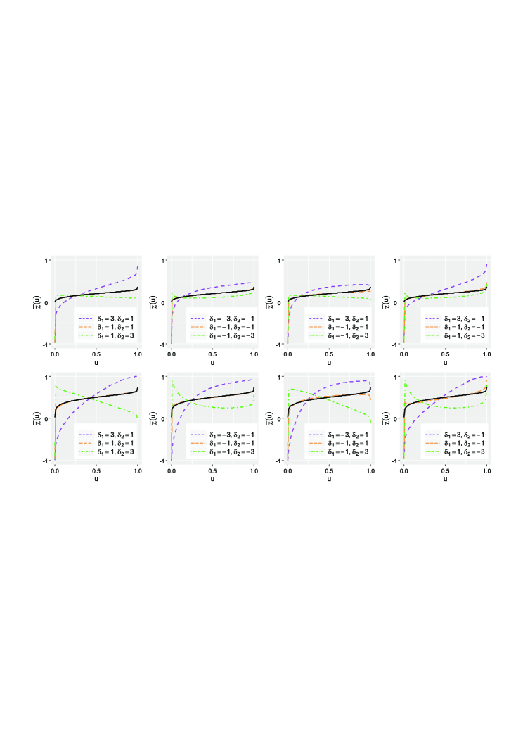
Figure 1: The dependence measure $\bar{\chi}(u)$ for the GSN distribution: the curves shown on first row correspond to $\rho=0.4$ as well as specified values of the $\delta_{i}$. The second row accords with $\rho=0.8$. The solid line in each panel corresponds to the normal distribution.

Under the asymptotic independence, Coles et al. (1999) recommended to characterize the extremal dependence at finite upper levels by

$$\bar{\chi}(u)=\frac{2\ln(P[F_{1}(Z_{1})>u])}{\ln(P[F_{1}(Z_{1})>u,F_{2}(Z_{2})>u])}-1,$$

where $-1\leq\bar{\chi}(u)\leq 1$ for all $0\leq u\leq 1$ and its larger magnitudes correspond to stronger dependence. (1) illustrate how the tail probabilities under the given GSN distribution in (3) varies with different values of the correlation parameter $\rho$ and various choices of the skewness parameters $\delta_{i}$.

These figures reveal a large variety of tail behaviours with different decay or increase rates. One can see that the sign change of skewness parameters results in conflicting shapes of the curves such as position of the curves relative to the Gaussian counterpart and dense or sparse behaviour. Another remark is that the tail probabilities of the GSN distribution in terms of $\bar{\chi}(u)$ is not always an increasing function of the correlation parameter. The special cases in these figures, in light of Proposition 2.1, are the ones with $0\leq\delta_{2}<\delta_{1}$ and $\delta_{2}<0\leq\delta_{1}$ which indicates some evidence for asymptotic dependence. Lastly, they manifestly exhibit positive extremal dependence while the negative and near dependence is appeared to a lesser extent under the current setting. Overall, these findings indicate that this version of GSN distribution can induce tail dependence at sub-asymptotic and/or asymptotic levels. The strength of dependence appears to vary with correlation as well as separation of skewness parameters. Of course, the parameters value $\delta_{1}=0$ and $\delta_{2}=0$ display null extremal dependence. Notably, the tail probabilities of all pairs of variables under the GSN distribution is not driven by a single parameter like a multivariate t distribution whose UTDC converges to the positive value for finite value of the degrees of freedom parameter regardless of the correlation parameter (Demarta and McNeil, 2005).

The numerical integration is implemented using the statistical software R (R Core Team, 2018). The computation of the $\bar{\chi}(\cdot)$ is restricted to the interval $[\zeta,1-\zeta]$, where $\zeta$ is defined by machine precision, about $10^{-9}$ on our machine.

3 The GSN distributed random field

A spatial RF model $\{Y(\mbox{\boldmath{$s$}}):\mbox{\boldmath{$s$}}\in\mathcal{D}\subset\mathbb{R}^{2}\}$ is a collection of random variables indexed via $\mbox{\boldmath{$s$}}\in\mathcal{D}$. If a finite set of locations $\{\mbox{\boldmath{$s$}}_{1},\ldots,\mbox{\boldmath{$s$}}_{n}\}\in\mathcal{D}$ is observed, then the finite-dimensional distributions for each $n\geq 1$ must satisfy Kolmogorov’s compatibility conditions. Using the mgf in (2), it can be shown that the compatibility conditions are satisfied under the GSN finite-dimensional distributions. Therefore, the GSN distributed RF is well-defined (Mahmoudian, 2018).

A key idea to link the GSN distribution and the spatial model is to view $Y$ as follows

$$Y(\mbox{\boldmath{$s$}})=\mu(\mbox{\boldmath{$s$}})+Z(\mbox{\boldmath{$s$}})+\epsilon(\mbox{\boldmath{$s$}}),$$ (4)

where $\mu(\mbox{\boldmath{$s$}})$, $Z(\mbox{\boldmath{$s$}})$ and $\epsilon(\mbox{\boldmath{$s$}})$ being location dependent mean function, a smooth-scale SGRF with

$${\rm GSN}_{n}(\mbox{\boldmath{$0$}},\mbox{\boldmath{$\Sigma$}},\mbox{\boldmath{$\delta$}})$$

finite-dimensional distribution and an i.i.d. (independent and identically distributed) GRF independent of $Z(\mbox{\boldmath{$s$}})$ with mean zero and variance $\tau^{2}$, respectively. The parameter $\tau^{2}$ is called nugget effect in geostatistical context. Equivalently, let that $\{W(\mbox{\boldmath{$s$}}):\mbox{\boldmath{$s$}}\in\mathbb{R}^{2}\}$ and $\{\delta(\mbox{\boldmath{$s$}}):\mbox{\boldmath{$s$}}\in\mathbb{R}^{2}\}$ be two stationary GRF defined on $\mathbb{R}^{2}$ and assume that $W(\mbox{\boldmath{$s$}})$ and $\delta(\mbox{\boldmath{$s$}})$ be independent, with components having following means

$${\rm E}[W(\mbox{\boldmath{$s$}})]=0,\quad{\rm E}[\delta(\mbox{\boldmath{$s$}})]=\gamma,\quad\mbox{\boldmath{$s$}}\in\mathbb{R}^{2},$$

and covariances

$${\rm Cov}[W(\mbox{\boldmath{$s$}}),W(\mbox{\boldmath{$s$}}^{\prime})]=\sigma^{2}\rho_{w}(||\mbox{\boldmath{$s$}}-\mbox{\boldmath{$s$}}^{\prime}||),\quad{\rm Cov}[\delta(\mbox{\boldmath{$s$}}),\delta(\mbox{\boldmath{$s$}}^{\prime})]=\gamma^{2}\rho_{\delta}(||\mbox{\boldmath{$s$}}-\mbox{\boldmath{$s$}}^{\prime}||),\quad\mbox{\boldmath{$s$}},\mbox{\boldmath{$s$}}^{\prime}\in\mathbb{R}^{2},$$ (5)

where $||\mbox{\boldmath{$s$}}-\mbox{\boldmath{$s$}}^{\prime}||$ is a Euclidean distance between two field measurement locations $s$ and $\mbox{\boldmath{$s$}}^{\prime}$. Furthermore, $\rho_{w}(\cdot)$ and $\rho_{\delta}(\cdot)$ in (5) are the corresponding spatial correlation functions of $W(\mbox{\boldmath{$s$}})$ and $\delta(\mbox{\boldmath{$s$}})$, respectively. Note that, under this formulation when distance between spatial locations goes to the infinity, the covariances of this SGRF vanish. One option for the correlation function is the Mat$\acute{\textrm{e}}$rn family of the correlation functions, given by

$$\rho(||\mbox{\boldmath{$s$}}-\mbox{\boldmath{$s$}}^{\prime}||;\psi,\xi)=\frac{1}{2^{\xi-1}\Gamma(\xi)}\left(\frac{1}{\psi}||\mbox{\boldmath{$s$}}-\mbox{\boldmath{$s$}}^{\prime}||\right)^{\xi}\mathcal{K}_{\xi}\left(\frac{1}{\psi}||\mbox{\boldmath{$s$}}-\mbox{\boldmath{$s$}}^{\prime}||\right),$$ (6)

where $\psi$ is a range parameter, $\Gamma(\cdot)$ is the gamma function and $\mathcal{K}_{\xi}(\cdot)$ is the modified Bessel function of the third kind of order $\xi>0$ (Stein, 1999). It depends on a smoothness parameter $\xi$ which directly controls the mean square differentiability of RF realizations. If $\xi>1$ then Mat$\acute{\textrm{e}}$rn correlation functions are once mean square differentiable, and if $\xi=3/2$, the correlation functions are of the closed form $(1+||\mbox{\boldmath{$s$}}-\mbox{\boldmath{$s$}}^{\prime}||/\psi)\exp(-||\mbox{\boldmath{$s$}}-\mbox{\boldmath{$s$}}^{\prime}||/\psi)$. Because parameters of the Mat$\acute{\textrm{e}}$rn correlation function often being poorly identified (Zhang, 2004), we set $\xi=3/2$. Under this setting, the range parameter $\psi$ is appeared out of the exponential term. Accordingly, data may contribute more information on estimation of $\psi$. Throughout the text, similar Mat$\acute{\textrm{e}}$rn correlation function with $\xi=3/2$ is adopted for each of $\rho_{w}(\cdot)$ and $\rho_{\delta}(\cdot)$ to ensure the existence of such GSN distributed RF model.

By assuming $T(\mbox{\boldmath{$s$}})=V(\mbox{\boldmath{$s$}})-\sqrt{2/\pi}$ and $V(\mbox{\boldmath{$s$}})\stackrel{{\scriptstyle\;\rm i.i.d.}}{{\sim}}{\rm HN}_{1}(0,1)$, one can employ the following representation of the spatial SGRF model

$$Y(\mbox{\boldmath{$s$}})=\mu(\mbox{\boldmath{$s$}})+W(\mbox{\boldmath{$s$}})+\delta(\mbox{\boldmath{$s$}})T(\mbox{\boldmath{$s$}})+\epsilon(\mbox{\boldmath{$s$}}).$$ (7)

Several properties of SGRF in the GSN family could be deduced from (7). Let us assume the case when the mean function is constant: $\mu(\mbox{\boldmath{$s$}})=\mu$ for all $\mbox{\boldmath{$s$}}\in\mathbb{R}^{2}$, then the skewed field defined in (7) is stationary with expectations

$${\rm E}[Y(\mbox{\boldmath{$s$}})]=\mu,\quad\mbox{\boldmath{$s$}}\in\mathbb{R}^{2},$$

variances

$${\rm Var}[Y(\mbox{\boldmath{$s$}})]=\tau^{2}+\sigma^{2}+2\gamma^{2}\left(1-\frac{2}{\pi}\right),\quad\mbox{\boldmath{$s$}}\in\mathbb{R}^{2},$$

and covariances

$${\rm Cov}[Y(\mbox{\boldmath{$s$}}),Y(\mbox{\boldmath{$s$}}^{\prime})]=\sigma^{2}{\rm\rho}_{w}(||\mbox{\boldmath{$s$}}-\mbox{\boldmath{$s$}}^{\prime}||),\quad\mbox{\boldmath{$s$}},\mbox{\boldmath{$s$}}^{\prime}\in\mathbb{R}^{2}.$$

4 Heavy-tailed construction of SGRF model

In this section, we consider the scale mixture of the GSN distributed RF model and discuss about its skewness and kurtosis. Let $Y_{i}=Y(\mbox{\boldmath{$s$}}_{i})$ denote the observation at spatial location $\mbox{\boldmath{$s$}}_{i}$ and consider the data model

$$Y_{i}=\mbox{\boldmath{$X$}}(\mbox{\boldmath{$s$}}_{i})^{\prime}\mbox{\boldmath{$\beta$}}+\sigma\lambda_{i}^{-1/2}W_{i}+\gamma\lambda_{i}^{-1/2}\delta_{i}T_{i}+\epsilon_{i},$$ (8)

where $X(\mbox{\boldmath{$s$}}_{i})$ is a $(p\times 1)$ vector of known location dependent covariates, $\beta$ is a $(p\times 1)$ vector of unknown regression parameters, $\sigma>0$ is the scale parameter, $\gamma\in\mathbb{R}$ is the asymmetry parameter and the spatial random effect $W_{i}=W(\mbox{\boldmath{$s$}}_{i})$ is independent of $T_{i}=T(\mbox{\boldmath{$s$}}_{i})$, follows a GRF model defined by

$$\mbox{\boldmath{$W$}}=(W_{1},\ldots,W_{n})^{\prime}\sim{\rm N}_{n}(0,\mbox{\boldmath{$H$}}),$$

where $H$ is a correlation matrix describing the spatial dependence, whose elements are given by (6) with $\xi=3/2$. The asymmetry parameter, $\gamma$, controls the direction and magnitude of skewness. It is worth recalling that negative values of $\gamma$ induce negative skewness, positive values generate positive skewness, and $\gamma=0$ corresponds to symmetry. To allow altered skewness mixing variable for each measurement location, by setting $\delta_{i}=\delta(\mbox{\boldmath{$s$}}_{i})$, we adopt the following GRF model for $\delta(\cdot)$:

$$\mbox{\boldmath{$\delta$}}=(\delta_{1},\ldots,\delta_{n})^{\prime}\sim{\rm N}_{n}(\mbox{\boldmath{$1$}}_{n},\mbox{\boldmath{$H$}}).$$

Also an additional set of latent random variables, $\lambda_{i}=\lambda(\mbox{\boldmath{$s$}}_{i})>0$, is introduced here to deal with the presence of outliers in the spatial responses. The scale mixing variables, $\mbox{\boldmath{$\lambda$}}=(\lambda_{1},\ldots,\lambda_{n})^{\prime}$, are assumed to be spatially correlated to induce the mean square continuity. Hence, $\lambda$ on the logarithm scale can be modeled by a GRF model as follows

$$\ln(\mbox{\boldmath{$\lambda$}})\sim{\rm N}_{n}\left(-\frac{\nu}{2}\mbox{\boldmath{$1$}}_{n},\nu\mbox{\boldmath{$H$}}\right),$$ (9)

where $\nu>0$ is the tail-weight parameter regulating the heaviness in tails of the RF. When the spatial model is rescaled according to the transformed GRF model in (9), on average the resultant finite-dimensional distribution is a GSN probability model with inflated variance. While large values of the tail-weight parameter has been found to provide heavier tails, the SGRF model corresponds to the limiting case when $\nu$ tends toward zero. Additionally, taking into account different correlation structures entails little flexibility in comparison to the skewness parameters. Therefore, we assume similar spatial correlation matrix for $\lambda(\cdot)$ and $W(\cdot)$. This assumption further can be assessed by analyzing real data sets in terms of better prediction results.

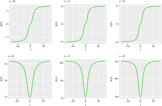
Figure 2: Coefficients of skewness (first row) and kurtosis (second row) for the model in (8) with respect to various values of the parameters $\gamma$ and $\nu$.

Now, we compute the coefficient of skewness and kurtosis of (8). Tedious but straightforward algebra proved that these coefficients are given, respectively, by

$${\rm S}(Y) =\frac{4\gamma^{3}\exp\left(\frac{15\nu}{8}\right)\left(\frac{4}{\pi}-1\right)\sqrt{\frac{2}{\pi}}}{\left[\tau^{2}+\sigma^{2}\exp(\nu)+2\gamma^{2}\exp(\nu)\left(1-\frac{2}{\pi}\right)\right]^{3/2}},$$

$${\rm K}(Y) =\frac{3\tau^{4}+3\sigma^{4}\exp(3\nu)+6\sigma^{2}\tau^{2}\exp(\nu)+12\sigma^{2}\gamma^{2}A_{1}+12\tau^{2}\gamma^{2}A_{2}+10\gamma^{4}A_{3}}{\left[\tau^{2}+\sigma^{2}\exp(\nu)+2\gamma^{2}\exp(\nu)\left(1-\frac{2}{\pi}\right)\right]^{2}},$$

in which

$$A_{1}=\exp(3\nu)\left(1-\frac{2}{\pi}\right),\quad A_{2}=\exp(\nu)\left(1-\frac{2}{\pi}\right),\quad A_{3}=\exp(3\nu)\left(3-\frac{4}{\pi}-\frac{12}{\pi^{2}}\right).$$

These measures are used to produce (2) which is plotted by varying $\gamma$ for different values of the parameter $\nu$ after assuming $\tau=1$ and $\sigma=1$, denoted by standard case. We do not introduce these parameters into the assessments, because they have minor impacts on skewness and kurtosis. Essentially, for fixed values of $\gamma$ and $\nu$, ${\rm S}(Y)$, and ${\rm K}(Y)$ decrease for increasing values of $\tau$ or $\sigma$. However, for large values of $\tau$ or $\sigma$, the skewness and kurtosis coefficients have similar patterns for greater values of $\gamma$ and $\nu$ than the ones that were assumed in the standard case. It can be examined when $\nu=0$, ${\rm S}(Y)$ varies in the interval $(-1.41,1.41)$, while ${\rm K}(Y)$ takes values in the range $(3,9.67)$. An aspect to be stressed right away is that the parameter $\nu$ ($\gamma$) is not concerned with tail (skewness) of the RF model merely. The addition of this extra parameter, $\nu$ ($\gamma$), to allow for flexibility in the GRF supports the skewness (tail) whose size expands with $\nu$ ($\gamma$). Consequently, both of $\nu$ and $\gamma$ control the non-Gaussian strength.

5 Conclusions

We extend the methodology previously presented in the literature to accurately incorporate size and direction of the skewness into the RF model. An elegant consequence is that the SGRF model with spatially varying skewness parameters do a great job in capturing tail probabilities which are thought to possess some degree of tail dependence.

References

- Apputhurai and Stephenson (2011) Apputhurai, P. and Stephenson, A.G., 2011. Accounting for uncertainty in extremal dependence modeling using Bayesian model averaging techniques. Journal of Statistical Planning and Inference 141, 1800-1807.
- Azzalini and Captianio (2014) Azzalini, A. and Captianio, A., 2014. The Skew-Normal and Related Families. IMS Monographs Series, Cambridge University Press.
- Beranger et al. (2019) Beranger, B., Padoan, S.A. and Xu, Y. and Sisson, S.A., 2019. Extremal properties of the multivariate extended skew-normal distribution, Part B. Statistics & Probability Letters 147, 105-114.
- Berger et al. (2001) Berger, J.O., De Oliveira, V. and Sans, B., 2001. Objective Bayesian analysis of spatially correlated data. Journal of the American Statistical Association 93 (456), 1361-1374.
- Bueno et al. (2017) Bueno, R.S., Fonseca, T.C.O. and Schmidt, A.M., 2017. Accounting for covariate information in the scale component of spatio-temporal mixing models. Spatial Statistics 22, 196-218.
- Coles et al. (1999) Coles, S., Heffernan, J. and Tawn, J., 1999. Dependence measures for extreme value analyses. Extremes 2 (4), 339-365.
- Cowles et al. (2009) Cowles, M.K., Yan, J. and Smith, B., 2009. Reparameterized and marginalized posterior and predictive sampling for complex Bayesian geostatistical models. Journal of Computational and Graphical Statistics 18 (2), 262-282.
- Davison et al. (2013) Davison, A.C., Huser, R. and Thibaud, E., 2013. Geostatistics of dependent and asymptotically independent extremes. Mathematical Geosciences 45 (5), 511-529.
- Demarta and McNeil (2005) Demarta, S. and McNeil, A.J., 2005. The t copula and related copulas. International Statistical Review 73, 111-129.
- Dey and Yan (2016) Dey, D.K. and Yan, J., 2016. Extreme Value Modeling and Risk Analysis: Methods and Applications. Boca Raton : CRC Press.
- Fagundes et al. (2018) Fagundes, R.S., Uribe-Opazo, M. A., Galea, M. and Guedes, L. P. C., 2018. Spatial variability in slash linear modeling with finite second moment. Journal of Agricultural, Biological and Environmental Statistics 23 (2), 276-296.
- Gelfand and Schliep (2016) Gelfand, A.E. and Schliep, E.M., 2016. Spatial statistics and Gaussian processes: a beautiful marriage. Spatial Statistics 18, 86-104.
- Genton and Zhang (2012) Genton, M. and Zhang, H., 2012. Identifiability problems in some non- Gaussian spatial random fields. Chilean Journal of Statistics 3, 171-179.
- Huser et al. (2017) Huser, R., Opitz, T. and Thibaud, E., 2017. Bridging asymptotic independence and dependence in spatial extremes using Gaussian scale mixtures. Spatial Statistics 21, 166-186.
- Huser and Wadsworth (2018) Huser, R. and Wadsworth, J.L., 2018. Modeling spatial processes with unknown extremal dependence class. Journal of the American Statistical Association, DOI: 10.1080/01621459.2017.1411813.
- Krupskii et al. (2018) Krupskii, P., Huser, R. and Genton, M.G., 2018. Factor copula models for replicated spatial data. Journal of the American Statistical Association 113 (521), 467-479.
- Lum and Gelfand (2012) Lum, K. and Gelfand, A.E., 2012. Spatial quantile multiple regression using the asymmetric Laplace process. Bayesian Analysis 7 (2), 235-258.
- Ma (2009) Ma, C., 2009. Construction of non-Gaussian random fields with any given correlation structure. Journal of Statistical Planning and Inference 139 (3), 780-787.
- Ma (2013) Ma, C., 2013. K-distributed vector random fields in space and time. Statistics & Probability Letters 83, 1143-1150.
- Mahmoudian (2017) Mahmoudian, B., 2017. A skewed and heavy-tailed latent random field model for spatial extremes. Journal of Computational and Graphical Statistics 26 (3), 658-670.
- Mahmoudian (2018) Mahmoudian, B., 2018. On the existence of some skew-Gaussian random field models. Statistics & Probability Letters 137, 331-335.
- Mahmoudian (2019) Mahmoudian, B., 2019. Non-Gaussian Bayesian geostatistical modeling of replicated spatial data. Under revision.
- Minozzo and Ferracuti (2012) Minozzo, M. and Ferracuti, L., 2012. On the existence of some skew- normal stationary processes. Chilean Journal of Statistics 3, 157-170.
- Morris et al. (2017) Morris, S.A., Reich, B.J., Thibaud, E. and Cooley, D., 2017. A space-time skew-t model for threshold exceedances. Biometrics, 73 (3), 749-758.
- Opitz (2016) Opitz, T., 2016. Modeling asymptotically independent spatial extremes based on Laplace random fields. Spatial Statistics 16, 1-18.
- Palacios and Steel (2006) Palacios, M.B. and Steel, M.F.J., 2006. Non-Gaussian Bayesian geostatistical modeling. Journal of the American Statistical Association 101 (474), 604-618.
- R Core Team (2018) R Core Team, 2018. R: A language and environment for statistical computing. R Foundation for Statistical Computing, Vienna, Austria. URL https://www.R-project.org/.
- Sahu et al. (2003) Sahu, S.K., Dey, D.K. and Branco, M.D., 2003. A new class of multivariate skew distributions with applications to Bayesian regression models. Canadian Journal of Statistics 31 (2), 129-150.
- Schmidt et al. (2017) Schmidt, A.M., Gonçalves, K.C.M. and Velozo, P.L., 2017. Spatiotemporal models for skewed processes. Environmetrics 28 (6), e2411.
- Stein (1999) Stein, M.L., 1999. Interpolation of Spatial Data: Some Theory for Kriging. New York: Springer-Verlag.
- Wadsworth et al. (2017) Wadsworth, J.L., Tawn, J.A., Davison, A.C. and Elton, D.M., 2017. Modelling across extremal dependence classes. Journal of the Royal Statistical Society, Series B 79 (1), 149-175.
- Xu and Genton (2017) Xu, G. and Genton, M., 2017. Tukey g-and-h random fields. Journal of the American Statistical Association 112 (519), 1236-1249.
- Zhang (2004) Zhang, H., 2004. Inconsistent estimation and asymptotically equal interpolations in model-based geostatistics. Journal of the American Statistical Association 99 (465), 250-261.
- Zhang and El-Shaarawi (2010) Zhang, H. and El-Shaarawi, A., 2010. On spatial skew-Gaussian processes and applications. Environmetrics 21 (1), 33-47.