The Price of Anarchy in Routing Games as a Function of the Demand

Abstract.

The price of anarchy has become a standard measure of the efficiency of equilibria in games. Most of the literature in this area has focused on establishing worst-case bounds for specific classes of games, such as routing games or more general congestion games. Recently, the price of anarchy in routing games has been studied as a function of the traffic demand, providing asymptotic results in light and heavy traffic. The aim of this paper is to study the price of anarchy in nonatomic routing games in the intermediate region of the demand. To achieve this goal, we begin by establishing some smoothness properties of Wardrop equilibria and social optima for general smooth costs. In the case of affine costs we show that the equilibrium is piecewise linear, with break points at the demand levels at which the set of active paths changes. We prove that the number of such break points is finite, although it can be exponential in the size of the network. Exploiting a scaling law between the equilibrium and the social optimum, we derive a similar behavior for the optimal flows. We then prove that in any interval between break points the price of anarchy is smooth and it is either monotone (decreasing or increasing) over the full interval, or it decreases up to a certain minimum point in the interior of the interval and increases afterwards. We deduce that for affine costs the maximum of the price of anarchy can only occur at the break points. For general costs we provide counterexamples showing that the set of break points is not always finite.

1. Introduction

Nonatomic routing games provide a model for the distribution of traffic over networks with a large number of drivers, each one representing a negligible fraction of the total demand. The model is based on a directed graph with one or more origin-destination pairs, and the costs are identified with the delays incurred to go from origin to destination. The delay on an edge is a nondecreasing function of the load of players on that edge, and the delay of a path is additive over its edges. The standard solution concept for such nonatomic games is the Wardrop equilibrium, according to which the traffic in each origin-destination (OD) pair travels along paths of minimum delay. The aggregate social cost experienced by the whole traffic is therefore the product of these minimal delays multiplied by the corresponding traffic demands, summed over all OD pairs.

Equilibria are known to be inefficient, so that a social planner would be able to reduce the social cost by redirecting flows along the network. The most common measure of inefficiency is the price of anarchy (PoA), that is, the ratio of the social cost at equilibrium over the minimum social cost. For nonatomic congestion games with affine costs, the value of the price of anarchy (PoA) is bounded above by $4/3$, and this bound is known to be sharp (Roughgarden and Tardos,, 2002). On the other hand, for a large class of cost functions, including all polynomials, the PoA converges to $1$ as the traffic demand goes either to $0$ or to infinity. In other words, equilibria tend to perfect efficiency both in light and heavy traffic (Colini-Baldeschi et al.,, 2020, Wu et al.,, 2021).

Empirical studies have shown that in real networks, and for intermediate levels of the demand, the PoA tends to oscillate and often does not reach the worst case bounds.

(a) A simple network with affine costs

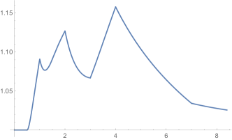
(b) PoA as a function of the traffic demand

Figure 1. Oscillations of the price of anarchy

Figure 1 shows a typical profile of the PoA as a function of the traffic demand. It starts at 1 for low levels of traffic, then it exhibits some oscillations with a number of nonsmooth spikes, and eventually it decreases smoothly back to 1 in the highly congested regime. The shape and number of these oscillations and spikes is the object of this paper.

1.1. Our contribution

We consider nonatomic routing games over a network with a single OD, and we study the behavior of the price of anarchy as a function of the traffic demand.

To achieve our goal, we need some general results on the continuity and monotonicity of the equilibrium costs and flows. We resort to the classical result in Beckmann et al., (1956) according to which a Wardrop equilibrium is a solution of a convex optimization program. We show that the optimal value of this program is convex and continuously differentiable as a function of the demand, and its derivative is precisely the equilibrium cost. A similar result is established for the minimum social cost.

When the costs have a strictly positive derivative, we show that the equilibrium loads and the PoA are in fact $C^{1}$ at each demand level that is regular, in the sense that all the optimal paths carry a strictly positive flow. This regularity fails in particular at the so-called $\widehat{\mathcal{E}}$-breakpoints, which are demand levels at which the set of shortest paths at equilibrium changes.

For affine costs we bypass regularity and we show directly that the equilibrium cost is piecewise linear and differentiable except at $\widehat{\mathcal{E}}$-breakpoints. The crucial property is that if the set of shortest paths is the same at two demand levels, then this set remains optimal in between. From here it follows that the number of $\widehat{\mathcal{E}}$-breakpoints is finite, though it can be exponentially large. It also follows that between $\widehat{\mathcal{E}}$-breakpoints the PoA is differentiable and either is monotone, or is first decreasing and then increasing, so it has a unique minimum in the interior of the interval. From this we conclude that the maximum of the PoA is attained at an $\widehat{\mathcal{E}}$-breakpoint.

We finally present several examples showing how these properties might fail for general costs.

1.2. Related Work

The standard solution concept in nonatomic routing games is due to Wardrop, (1952). Its mathematical properties were first studied by Beckmann et al., (1956); early algorithms for computing equilibria were proposed by Tomlin, (1966) for affine costs, and by Dafermos and Sparrow, (1969) for general convex costs. For historical surveys on the topic we refer to Florian and Hearn, (1995) as well as Correa and Stier-Moses, (2011).

Several papers have considered the sensitivity of the equilibrium flows and costs with respect to variations of the traffic demand. Hall, (1978) showed that an increase in the demand of one OD pair always increases the equilibrium cost for that pair, whereas Fisk, (1979) observed that the cost on a different OD could be reduced. These questions were further explored by Dafermos and Nagurney, (1984). In a different direction, Patriksson, (2004) characterized the existence of directional derivatives for the equilibrium. Josefsson and Patriksson, (2007) proved that equilibrium costs are always directionally differentiable, whereas equilibrium edge loads not always are. Englert et al., (2010) showed that there exist single OD network games where an $\varepsilon$-increase in the traffic demand produces a global migration of traffic from one set of equilibrium paths to a disjoint set of paths, but, nevertheless, the load on each edge changes at most by $\varepsilon$. Moreover, if the cost functions are polynomials of degree at most $d$, then the equilibrium costs increase at most of a multiplicative factor $(1+\varepsilon)^{d}$. Takalloo and Kwon, (2020) extended this last result to games with multiple OD pairs.

The recognition that selfish behavior produces social inefficiency goes back at least to Pigou, (1920). A measure to quantify this inefficiency was proposed by Koutsoupias and Papadimitriou, (1999), by considering the ratio of the social cost of the worst equilibrium over the optimum social cost. It was termed price of anarchy by Papadimitriou, (2001). A PoA close to one indicates efficiency of the equilibria of the game, whereas a high PoA implies that, in the worst scenario, strategic behavior can lead to significant social inefficiency. Most of the subsequent literature established sharp bounds for the PoA for specific classes of games, notably for congestion games and in particular for routing games. Roughgarden and Tardos, (2002) showed that in every nonatomic congestion game with affine costs the PoA is bounded above by $4/3$. Moreover, this bound is sharp and attained in a traffic game with a simple two-edge parallel network. Roughgarden, (2003) generalized this result to polynomial functions of maximum degree $d$ showing that the PoA grows as $\Theta(d/\log d)$. Dumrauf and Gairing, (2006) refined the result when the cost functions are sums of monomials whose degrees are between $q$ and $d$. Roughgarden and Tardos, (2004) extended the analysis to all differentiable cost function $c$ such that $xc(x)$ is convex. Less regular costs and different optimizing criteria for the social cost were studied by Correa et al., (2008, 2004, 2007).

Some papers took a more applied view and studied the actual value of the PoA in real networks. Youn et al., (2008, 2009) dealt with traffic in Boston, London, and New York, and noted that the PoA exhibits a similar pattern in the three cities: it is $1$ when traffic is light, it oscillates in the central region and then goes back to $1$ when traffic increases. A similar behavior was observed by O’Hare et al., (2016), who—taking an approach that relates to the one in this paper—showed how an expansion and/or retraction of the routes used at equilibrium affects the behavior of the PoA. Experimentally, Monnot et al., (2017) studied the commuting behavior of a large number of Singaporean students and concluded that the PoA is overall low and far from the worst case scenarios.

An analytical justification for the asymptotic efficiency of the PoA in light and heavy traffic was presented in Colini-Baldeschi et al., (2019, 2020), Wu et al., (2021). Colini-Baldeschi et al., (2019) considered the case of single OD parallel networks and proved that, in heavy traffic, the PoA converges to one when the cost functions are regularly varying. Their results were extended in various directions in Colini-Baldeschi et al., (2020), considering general networks and analyzing both the light and heavy traffic asymptotics. A different technique, called scalability, was used by Wu et al., (2021) to study the case of heavy traffic.

Wu and Möhring, (2020) considered issues that are quite close to the one examined here. They defined a metric on the space of nonatomic congestion games that share the same network, commodities, and strategies, but differ in terms of demands and cost functions. Using this metric they showed that the PoA is a continuous function of both the demand and the costs. Then they performed a sensitivity analysis of the PoA with respect to variations of the game in terms of this metric.

In a very interesting recent paper Klimm and Warode, (2021) (see also the conference version Klimm and Warode,, 2019) consider nonatomic routing games with piecewise linear costs and present algorithms to track the full path of Wardrop equilibria when the demands vary proportionally along a fixed direction. These algorithms are based on (positive or negative) electrical flows on undirected graphs and are then suitably adapted to positive flows on directed graphs. The connection between their paper and ours will be discussed in Section 4.

The behavior of the PoA as a function of a different parameter was studied by Cominetti et al., (2019). In that case the parameter of interest was the probability that players actually take part in the game. Colini-Baldeschi et al., (2018) studied the possibility of achieving efficiency in routing games via the use of tolls, when the demand can vary, while Gemici et al., (2019) analyzed the income inequality effects of reducing the PoA via tolls.

1.3. Organization of the paper

In Section 2 we recall the model of nonatomic routing games, and we set the notations and the standing assumptions. Section 3 investigates the smoothness of the equilibrium costs and of the PoA as a function of the demand, for general nondecreasing smooth costs. The behavior of the PoA for affine costs is studied in Section 4. Section 5 presents various examples.

2. The nonatomic congestion model

We consider a nonatomic routing game with a single origin-destination pair. The network is described by a directed multigraph $\mathcal{G}=(\mathcal{V},\mathcal{E})$ with vertex set $\mathcal{V}$, edge set $\mathcal{E}$, an origin $O\in\mathcal{V}$, and a destination $D\in\mathcal{V}$. The traffic demand is given by a positive real number $\mu>0$, interpreted as vehicles per hour, which has to be routed along a set $\mathcal{P}$ of simple paths from $O$ to $D$. The nonatomic hypothesis means that each vehicle controls a negligible fraction of the total traffic, and consequently the traffic flows are treated as continuous variables.

The traffic flow on path $p$ is denoted by $f_{p}$ and the set of feasible flow profiles is

$$\mathcal{F}_{\mu}=\left\{\boldsymbol{f}=(f_{p})_{p\in\mathcal{P}}\colon f_{p}\geq 0\text{ and }\sum_{p\in\mathcal{P}}f_{p}=\mu\right\}.$$ (2.1)

Each flow profile $\boldsymbol{f}\in\mathcal{F}_{\mu}$ induces a load profile $\boldsymbol{x}=(x_{e})_{e\in\mathcal{E}}$ with $x_{e}=\sum_{p\ni e}f_{p}$ representing the aggregate traffic over the edge $e$. We call $\mathcal{X}_{\mu}$ the set of all such load profiles. Note that different flow profiles may induce the same edge loads so this correspondence is not bijective.

Every edge $e\in\mathcal{E}$ has a continuous nondecreasing cost function $c_{e}\colon[0,+\infty)\to[0,+\infty)$, where $c_{e}(x_{e})$ represents the travel time (or unit cost) of traversing the edge when the load is $x_{e}$. When the traffic is distributed according to $\boldsymbol{f}=(f_{p})_{p\in\mathcal{P}}$ with induced load profile $\boldsymbol{x}=(x_{e})_{e\in\mathcal{E}}$, the cost experienced by traveling on a path $p\in\mathcal{P}$ is given by

$$c_{p}(\boldsymbol{f})\coloneqq\sum_{e\in p}c_{e}\left(\sum_{p^{\prime}\ni e}f_{p^{\prime}}\right)=\sum_{e\in p}c_{e}(x_{e}).$$ (2.2)

With a slight abuse of notation, we use the same symbol $c$ for the cost function over paths and over edges. The meaning should be clear from the context.

2.1. Wardrop equilibrium

A feasible flow profile is called a Wardrop equilibrium if the paths that are actually used have minimum cost. Formally, $\boldsymbol{f}^{\ast}\in\mathcal{F}_{\mu}$ is an equilibrium iff there exists $\lambda\in\mathbb{R}$ such that

$$\begin{cases}c_{p}(\boldsymbol{f}^{\ast})=\lambda&\text{for each }p\in\mathcal{P}\text{ such that }f^{\ast}_{p}>0,\\ c_{p}(\boldsymbol{f}^{\ast})\geq\lambda&\text{for each }p\in\mathcal{P}\text{ such that }f^{\ast}_{p}=0.\end{cases}$$ (2.3)

The quantity $\lambda$ is called the equilibrium cost, and is a function of $\mu$.

As noted by Beckmann et al., (1956), Wardrop equilibria coincide with the optimal solutions of the convex minimization problem

$$V(\mu)\coloneqq\min_{\boldsymbol{f}\in\mathcal{F}_{\mu}}\sum_{e\in\mathcal{E}}C_{e}\left(\sum_{p^{\prime}\ni e}f_{p^{\prime}}\right)=\min_{x\in\mathcal{X}_{\mu}}\sum_{e\in\mathcal{E}}C_{e}(x_{e}),$$ (2.4)

where $C_{e}(\,\cdot\,)$ is the primitive of the edge cost $c_{e}(\,\cdot\,)$, that is,

$$C_{e}(x_{e})=\int_{0}^{x_{e}}\!\!c_{e}(z)\ \textup{d}z.$$ (2.5)

This follows by noting that (2.3) are the optimality conditions for $V(\mu)$, with the equilibrium cost $\lambda$ playing the role of a Lagrange multiplier for the constraint $\sum_{p}f_{p}=\mu$. It follows that, for each fixed demand $\mu$ an equilibrium flow $\boldsymbol{f}^{\ast}$ always exists.

Although Wardrop equilibria are not always unique, all of them induce the same edge costs $\tau_{e}(\mu)\coloneqq c_{e}(x^{\ast}_{e})$. In particular they have the same equilibrium cost $\lambda=\lambda(\mu)$, which is simply the shortest $O$-$D$ distance:

$$\lambda(\mu)=\min_{p\in\mathcal{P}}\sum_{e\in p}\tau_{e}(\mu).$$ (2.6)

As a matter of fact, as proved by Fukushima, (1984), the equilibrium edge costs $\tau_{e}=\tau_{e}(\mu)$ are the unique optimal solution of the strictly convex dual program

$$\min_{\tau}\sum_{e\in\mathcal{E}}C_{e}^{*}(\tau_{e})-\mu\,\min_{p\in\mathcal{P}}\sum_{e\in p}\tau_{e}$$ (2.7)

where $C_{e}^{*}(\,\cdot\,)$ is the Fenchel conjugate of $C_{e}(\,\cdot\,)$, which is strictly convex.

2.2. Social optimum and efficiency of equilibria

The total cost experienced by all users traveling across the network is called the social cost and is denoted by

$$\operatorname{\mathsf{SC}}(\boldsymbol{f})\coloneqq\sum_{p\in\mathcal{P}}f_{p}\,c_{p}(\boldsymbol{f})=\sum_{e\in\mathcal{E}}x_{e}\,c_{e}(x_{e}).$$ (2.8)

Since in equilibrium all the paths that carry flow have the same cost $\lambda(\mu)$, it follows that all equilibria have the same social cost, that is,

$$\operatorname{\mathsf{SC}}(\boldsymbol{f}^{\ast})=\sum_{p\in\mathcal{P}}f^{\ast}_{p}\,c_{p}(\boldsymbol{f}^{\ast})=\sum_{p\in\mathcal{P}}f^{\ast}_{p}\,\lambda(\mu)=\mu\,\lambda(\mu).$$ (2.9)

A feasible flow $\widetilde{\boldsymbol{f}}\in\mathcal{F}_{\mu}$ is called an optimum flow if it minimizes the social cost, that is, $\widetilde{\boldsymbol{f}}$ is an optimal solution of

$$\widetilde{V}(\mu)\coloneqq\min_{\boldsymbol{f}\in\mathcal{F}_{\mu}}\operatorname{\mathsf{SC}}(\boldsymbol{f})=\min_{\boldsymbol{f}\in\mathcal{F}_{\mu}}\sum_{e\in\mathcal{E}}\widetilde{C}_{e}\left(\sum_{p^{\prime}\ni e}f_{p^{\prime}}\right),$$ (2.10)

where $\widetilde{C}_{e}(x_{e})=x_{e}\,c_{e}(x_{e})$. The price of anarchy (PoA) is then defined as the ratio between the social cost at equilibrium $\mu\,\lambda(\mu)$ and the minimum social cost $\widetilde{V}(\mu)$:

$$\operatorname{\mathsf{PoA}}(\mu)=\frac{\mu\,\lambda(\mu)}{\widetilde{V}(\mu)}.$$ (2.11)

Our main goal is to investigate the smoothness of the function $\mu\mapsto\operatorname{\mathsf{PoA}}(\mu)$ and to understand the kinks and monotonicity properties observed in the example of Fig. 1(b). To this end, Section 3 presents some preliminary results on the differentiability of equilibria as a function of the demand $\mu$. More precise results will be discussed in Section 4 for the case with affine costs.

3. Differentiability of equilibria and price of anarchy

In order to study the smoothness of the PoA, we begin by establishing some preliminary facts on the differentiability of the optimal value function $\mu\mapsto V(\mu)$ and the smoothness of the equilibrium loads $\mu\mapsto x^{\ast}_{e}(\mu)$. These results follow from general convex duality and sensitivity analysis of parametric optimization problems. The following property does not seem to have been stated earlier in the literature, at least in this generality.

Proposition 3.1.

The map $\mu\mapsto V(\mu)$ is convex and $C^{1}$ on $(0,\infty)$ with $V^{\prime}(\mu)=\lambda(\mu)$ continuous and nondecreasing. Moreover, the equilibrium costs $\tau_{e}(\mu)$ are uniquely defined and continuous.

Proof.

This is a consequence of the convex duality theorem. Indeed, consider the perturbation function $\varphi_{\mu}:\mathbb{R}^{|\mathcal{P}|}\times\mathbb{R}\to\mathbb{R}\cup\{+\infty\}$, given by

$$\varphi_{\mu}(\boldsymbol{f},z)=\begin{cases}\sum_{e\in\mathcal{E}}c_{e}\left(\sum_{p^{\prime}\ni e}f_{p^{\prime}}\right)&\text{if }\boldsymbol{f}\geq\boldsymbol{0},\ \sum_{p}f_{p}=\mu+z\\ +\infty&\text{otherwise}.\end{cases}$$ (3.1)

Clearly $\varphi_{\mu}$ is a proper closed convex function (Rockafellar,, 1997, page 24). Calling

$$v_{\mu}(z)=\inf_{\boldsymbol{f}}\varphi_{\mu}(\boldsymbol{f},z),$$ (3.2)

we have $V(\mu+z)=v_{\mu}(z)$ and in particular $V(\mu)=v_{\mu}(0)$ which we consider as the primal problem $(\mathsf{P}_{\mu})$. From general convex duality, we have that $z\mapsto v_{\mu}(z)=V(\mu+z)$ is a convex function, from which we deduce that $V(\,\cdot\,)$ is convex. Moreover, the perturbation function $\varphi_{\mu}$ yields a corresponding dual

$$(\mathsf{D}_{\mu})\quad\min_{\lambda\in\mathbb{R}}\varphi_{\mu}^{*}(\boldsymbol{0},\lambda),$$ (3.3)

where $\varphi_{\mu}^{*}$ is the Fenchel conjugate function, that is,

$$\varphi_{\mu}^{*}(\boldsymbol{0},\lambda) =\sup_{\boldsymbol{f},z}~{}\langle\boldsymbol{0},\boldsymbol{f}\rangle+\lambda z-\varphi_{\mu}(\boldsymbol{f},z)$$

$$=\sup_{\boldsymbol{f}\geq\boldsymbol{0}}\lambda\left(\sum_{p}f_{p}-\mu\right)-\sum_{e\in\mathcal{E}}C_{e}\left(\sum_{p^{\prime}\ni e}f_{p^{\prime}}\right).$$

Since $V(\mu^{\prime})$ is finite for all $\mu^{\prime}\in(0,\infty)$, it follows that $v_{\mu}(z)=V(\mu+z)$ is finite for $z$ in some interval around $0$, and then the convex duality theorem implies that there is no duality gap and the subdifferential $\partial v_{\mu}(0)$ at $z=0$ coincides with the optimal solution set $\mathsf{S}(\mathsf{D}_{\mu})$ of the dual problem, that is, $\partial V(\mu)=\partial v_{\mu}(0)=\mathsf{S}(\mathsf{D}_{\mu})$.

We claim that the dual problem has a unique solution, which is exactly the equilibrium cost $\lambda(\mu)$. Indeed, fix an optimal solution $\boldsymbol{f}^{\ast}$ for $v_{\mu}(0)=V(\mu)$ and recall that this is just a Wardrop equilibrium. The dual optimal solutions are precisely the $\lambda$’s such that

$$\varphi_{\mu}(\boldsymbol{f}^{\ast},0)+\varphi_{\mu}^{*}(\boldsymbol{0},\lambda)=0.$$

This equation can be written explicitly as

$$\sum_{e\in\mathcal{E}}C_{e}\left(\sum_{p\ni e}f^{\ast}_{p}\right)+\sup_{\boldsymbol{f}\geq\boldsymbol{0}}~{}\lambda\left(\sum_{p}f_{p}-\mu\right)-\sum_{e\in\mathcal{E}}C_{e}\left(\sum_{p^{\prime}\ni e}f_{p^{\prime}}\right)=0,$$

from which it follows that $\boldsymbol{f}=\boldsymbol{f}^{\ast}$ is an optimal solution in the latter supremum. The corresponding optimality conditions are

$$\lambda-\sum_{e\in p}c_{e}\left(\sum_{p^{\prime}\ni e}f^{\ast}_{p^{\prime}}\right)=0, \quad\text{ if }f^{\ast}_{p}>0,$$

$$\lambda-\sum_{e\in p}c_{e}\left(\sum_{p^{\prime}\ni e}f^{\ast}_{p^{\prime}}\right)\leq 0, \quad\text{ if }f^{\ast}_{p}=0,$$

which imply that $\lambda$ is the equilibrium cost for the Wardrop equilibrium, that is, $\lambda=\lambda(\mu)$. It follows that $\partial V(\mu)=\{\lambda(\mu)\}$ so that $\mu\mapsto V(\mu)$ is not only convex but also differentiable with $V^{\prime}(\mu)=\lambda(\mu)$. The conclusion follows by noting that every convex differentiable function is automatically of class $C^{1}$, with $V^{\prime}(\mu)$ nondecreasing.

The continuity of the equilibrium edge costs $\tau_{e}=\tau_{e}(\mu)$ is a consequence of Berge’s maximum theorem (see, e.g., Aliprantis and Border,, 2006, Section 17.5). Indeed, the equilibrium edge costs are optimal solutions for the dual program in Eq. 2.7. Since the objective function is jointly continuous in $(\tau,\mu)$, Berge’s theorem implies that the optimal solution correspondence is upper-semicontinous. However, in this case the optimal solution is unique, so that the optimal correspondence is single-valued, and, as a consequence, the equilibrium edge costs $\tau_{e}(\mu)$ are continuous. ∎

As an immediate consequence of Proposition 3.1 we obtain the following result:

Corollary 3.2.

If the costs $c_{e}(\,\cdot\,)$ are strictly increasing and continuous, the equilibrium loads $x^{\ast}_{e}(\mu)=c_{e}^{-1}(\tau_{e}(\mu))$ are unique and continuous.

For multiple origin-destination networks with continuous and strictly increasing costs, the continuity of the equilibrium loads $x^{\ast}_{e}$ as a function of the demands was already proved in Hall, (1978, Theorem 1). On the other hand, Hall, (1978, Theorem 2) proved the continuity of the equilibrium costs provided that all paths carry a strictly positive flow, while Hall, (1978, Theorem 3) showed that the equilibrium cost of each OD increases with the corresponding demand. As shown in Proposition 3.1, for a single origin-destination the continuity and monotonicity of the equilibrium cost requires neither that costs be strictly increasing nor that all paths carry a strictly positive flow. Although this might be considered a minor improvement, allowing for nondecreasing costs and particularly constant costs is a convenient extension.

For the analysis of the PoA, the most relevant part of Proposition 3.1 is the smoothness of $V(\,\cdot\,)$ and the characterization of its derivative $V^{\prime}(\mu)=\lambda(\mu)$. In particular, considering the social optimum problem (2.10) we get the following direct consequence:

Proposition 3.3.

Let the costs $c_{e}(\,\cdot\,)$ be $C^{1}$ and nondecreasing with $x_{e}\mapsto x_{e}\,c_{e}(x_{e})$ convex. Then the optimal social cost $\mu\mapsto\widetilde{V}(\mu)$ is convex and $C^{1}$. Moreover, $\mu\mapsto\operatorname{\mathsf{PoA}}(\mu)$ is continuous in $(0,+\infty)$ and differentiable at every $\mu$ where the equilibrium cost $\lambda(\mu)$ is differentiable.

Proof.

The assumptions on $c_{e}(\,\cdot\,)$ imply that the marginal costs

$$\widetilde{c}_{e}(x_{e})\coloneqq\widetilde{C}_{e}^{\prime}(x_{e})=c_{e}(x_{e})+x_{e}\,c_{e}^{\prime}(x_{e})$$ (3.4)

are continuous and nondecreasing. It follows that the optimal flows are the Wardrop equilibria for these marginal costs, and the smoothness of $\widetilde{V}(\mu)$ follows from Proposition 3.1. For the PoA it suffices to observe that $\lambda(\mu)$ is continuous and then use the equality (2.11). ∎

Wu and Möhring, (2020) recently established a very general result on the continuity of the PoA with respect to the demands and also with respect to perturbations of the cost functions. However, differentiability was not addressed in their paper.

3.1. Differentiability of equilibrium costs

In order to use Proposition 3.3 it is convenient to find conditions that ensure the differentiability of the equilibrium cost $\lambda(\mu)$. In this section we present one such result, which also guarantees the differentiability of the resource loads $x^{\ast}_{e}(\mu)$. This follows from the implicit function theorem applied to the system of first order optimality conditions for Eq. 2.4. Given a vertex $v\in\mathcal{V}$, call $\mathcal{N^{+}}(v)$ and $\mathcal{N^{-}}(v)$ the sets of out-edges and in-edges of $v$, respectively, and $\mathcal{P}(O,v)$ the set of all paths from $O$ to $v$. Moreover, call $\mathcal{E}\left(v,w\right)$ the set of all edges $e\in\mathcal{E}$ that go from $v$ to $w$. Then, an equilibrium load profile $(x^{\ast}_{e})_{e\in\mathcal{E}}$ for a total demand $\mu$ is characterized as a solution of

$$x_{e}\geq 0~{}\text{ for all }~{}e\in\mathcal{E},$$ (3.5)

$$\sum_{e\in\mathcal{N^{+}}(v)}x_{e}-\sum_{e\in\mathcal{N^{-}}(v)}x_{e}=\begin{cases}~{}~{}0&\text{ if }v\neq O,D,\\ ~{}~{}\mu&\text{ if }v=O,\\ -\mu&\text{ if }v=D,\end{cases}\quad\text{for all }v\in\mathcal{V},$$ (3.6)

$$T_{O}=0~{}\text{ and }~{}T_{w}\leq T_{v}+\tau_{e}~{}\text{ for all }~{}e\in\mathcal{E}(v,w),$$ (3.7)

$$x_{e}\cdot(T_{w}-T_{v}-\tau_{e})=0~{}\text{ for all }~{}e\in\mathcal{E}(v,w),$$ (3.8)

$$\tau_{e}=c_{e}(x_{e})~{}\text{ for all }~{}e\in\mathcal{E},$$ (3.9)

where $\tau_{e}$ is the equilibrium cost of the edge $e$ and

$$T_{v}\coloneqq\min_{p\in\mathcal{P}(O,v)}\sum_{e\in p}\tau_{e}$$ (3.10)

is the equilibrium cost of a shortest path from the origin $O$ to vertex $v$.

For the subsequent analysis we define the active network as the set of all edges that lie on some shortest path. We also consider the demand levels at which this set changes.

Definition 3.4.

For each $\mu>0$ we let $\mathcal{P}(\mu)$ be the set of all shortest paths from the source $O$ to the sink $D$ with cost at equilibrium equal to $\lambda(\mu)$, and we define the active network $\widehat{\mathcal{E}}(\mu)$ as the union of the edges on all these paths $p\in\mathcal{P}(\mu)$.

The active network is said to be locally constant at $\mu_{0}$ if there exists $\varepsilon>0$ such that $\widehat{\mathcal{E}}(\mu)$ is the same for all $\mu\in[\mu_{0}-\varepsilon,\mu_{0}+\varepsilon]$.

The demand $\mu_{0}$ is called an $\widehat{\mathcal{E}}$-breakpoint if there exists $\varepsilon>0$ such that $\widehat{\mathcal{E}}(\mu)$ is constant over each of the intervals $[\mu_{0}\!-\!\varepsilon,\mu_{0})$ and $(\mu_{0},\mu_{0}\!+\!\varepsilon]$, with $\widehat{\mathcal{E}}(\mu_{0}\!-\!\varepsilon)\neq\widehat{\mathcal{E}}(\mu_{0}\!+\!\varepsilon)$.

Remark 3.1.

Since the equilibrium costs $\tau_{e}=\tau_{e}(\mu)$ and $\lambda(\mu)$ are unique for each $\mu$, it follows that both $\mathcal{P}(\mu)$ and $\widehat{\mathcal{E}}(\mu)$ are also uniquely determined. Moreover, the continuity of $\tau_{e}(\mu)$ implies that an edge $e\not\in\widehat{\mathcal{E}}(\mu_{0})$ that is inactive at $\mu_{0}$ remains inactive for $\mu$ near $\mu_{0}$, that is to say $\widehat{\mathcal{E}}(\mu_{0})^{c}\subseteq\widehat{\mathcal{E}}(\mu)^{c}$.

Fig. 2 shows the evolution of the active network at different demand levels for the game in Fig. 1(a), with five $\widehat{\mathcal{E}}$-breakpoints at $\mu=1,2,3,4,7$. Notice the correspondence with the break points in the price of anarchy in Fig. 1(b).

(a) $0\leq\mu<1$

(b) $1\leq\mu<2$

(c) $2\leq\mu\leq 3$

(d) $3<\mu<4$

(e) $4\leq\mu\leq 7$

(f) $7<\mu<\infty$

Figure 2. The active network for the graph on Fig. 1, with $\widehat{\mathcal{E}}$-breakpoints at $\mu=1,2,3,4,7$.

Although in general there can be infinitely many $\widehat{\mathcal{E}}$-breakpoints (see Proposition 5.1 and Remark 5.1), their number is finite for series-parallel networks (cf. Proposition 3.10) and also for general networks with affine costs (cf. Proposition 4.2). In both cases, once an active network changes, it may never occur again at higher demand levels.

An edge carrying a strictly positive flow at equilibrium must be on some optimal path, and, as a consequence, belongs to the active network. However, the converse may fail when a path becomes active but carries no flow. In order to prove the smoothness of the equilibrium flows we need to avoid this situation, which leads to the following definition of a regular demand.

Definition 3.5.

A demand $\mu>0$ is called regular if there is an equilibrium with $x_{e}>0$ for all $e\in\widehat{\mathcal{E}}(\mu)$.

Regularity is just strict complementarity. Indeed, the complementarity condition (3.8) imposes that for each $e\in\mathcal{E}$ either $x_{e}$ or $(T_{w}-T_{v}-\tau_{e})$ is zero, whereas strict complementarity requires exactly one of these expressions to be zero. As shown next, when the costs are strictly increasing this implies that the active network is locally constant, so that a regular demand cannot be an $\widehat{\mathcal{E}}$-breakpoint. We note however that there can be nonregular demands at which the active network is still locally constant (see Example 5.2).

Lemma 3.6.

Suppose that the costs $c_{e}(\,\cdot\,)$ are strictly increasing and continuous. If $\mu_{0}$ is a regular demand then the active network $\widehat{\mathcal{E}}(\mu)$ is locally constant at $\mu_{0}$.

Proof.

From regularity all active edges $e\in\widehat{\mathcal{E}}(\mu_{0})$ satisfy $x^{\ast}_{e}(\mu_{0})>0$. By Proposition 3.1 the maps $x^{\ast}_{e}(\,\cdot\,)$ are continuous, so these strict inequalities are preserved for $\mu$ near $\mu_{0}$, and therefore $\widehat{\mathcal{E}}(\mu_{0})\subseteq\widehat{\mathcal{E}}(\mu)$. This, combined with Remark 3.1, yields $\widehat{\mathcal{E}}(\mu)=\widehat{\mathcal{E}}(\mu_{0})$ for $\mu$ close to $\mu_{0}$. ∎

We are now ready to establish the smoothness of the equilibrium.

Proposition 3.7.

Assume that the costs $c_{e}(\,\cdot\,)$ are $C^{1}$ with strictly positive derivative. If $\mu_{0}$ is a regular demand then $\mu\mapsto(\boldsymbol{x}^{\ast}(\mu),\boldsymbol{\tau}(\mu),\boldsymbol{T}(\mu))$ is continuously differentiable in a neighborhood of $\mu_{0}$. In particular the equilibrium cost $\mu\mapsto\lambda(\mu)$ is $C^{1}$ near $\mu_{0}$.

Proof.

From Propositions 3.1 and 3.2, the equilibrium costs $\tau_{e}(\mu)$ and loads $x^{\ast}_{e}(\mu)$ are uniquely defined and continuous in $\mu$. Hence, the equilibrium cost $T_{v}(\mu)$ of a shortest path to any vertex $v$ is also continuous. These functions $x^{\ast}_{e},\tau_{e}$ and $T_{v}$ satisfy in particular Eqs. 3.6, 3.8 and 3.9.

Now, since $\mu_{0}$ is regular, the active network is locally constant. Let $\widehat{\mathcal{E}}_{0}=\widehat{\mathcal{E}}(\mu_{0})$ be this active network and $\mathcal{V}_{0}$ the corresponding vertices. Moreover, call $\widehat{\mathcal{E}}_{0}\left(v,w\right)$ the set of all edges $e\in\widehat{\mathcal{E}}_{0}$ that go from $v$ to $w$. For $\mu$ near $\mu_{0}$ we have $x^{\ast}_{e}(\mu)=0$ for all $e\not\in\widehat{\mathcal{E}}_{0}$; hence, these functions are trivially differentiable. Also for $w\not\in\mathcal{V}_{0}$ we can take $v\in\mathcal{V}_{0}$ the last vertex on a shortest path from $O$ to $w$, so that $T_{w}(\mu)=T_{v}(\mu)+\Delta_{v,w}$ where $\Delta_{v,w}$ is a constant travel time from $v$ to $w$. Hence it suffices to establish the smoothness of $x^{\ast}_{e}(\mu)$ for $e\in\widehat{\mathcal{E}}_{0}$ and $T_{v}(\mu)$ for $v\in\mathcal{V}_{0}$. To this end, consider Eqs. 3.6, 3.8 and 3.9 restricted to the edges in $\widehat{\mathcal{E}}_{0}$, together with the equation $T_{O}=0$, which gives the following system:

$$\sum_{e\in\mathcal{N^{+}}(v)\cap\widehat{\mathcal{E}}_{0}}x_{e}-\sum_{e\in\mathcal{N^{-}}(v)\cap\widehat{\mathcal{E}}_{0}}x_{e}=\begin{cases}0\text{ if }v\neq O,D,\\ \mu\text{ if }v=O,\end{cases}\quad\text{for all }v\in\mathcal{V}_{0},$$ (3.11)

$$x_{e}\cdot(T_{w}-T_{v}-\tau_{e})=0\quad\text{for all }e\in\widehat{\mathcal{E}}_{0}(v,w),$$ (3.12)

$$\tau_{e}=c_{e}(x_{e}),$$ (3.13)

$$T_{O}=0.$$ (3.14)

To apply the implicit function theorem to this reduced system, we must check that the associated linearized system has a unique solution. Let $u_{e}$, $\delta_{v}$ and $s_{e}$ be respectively the increments in the variables $x_{e}$, $T_{v}$ and $\tau_{e}$ for each $e\in\widehat{\mathcal{E}}_{0}$ and $v\in\mathcal{V}_{0}$. The homogeneous linear system obtained from Eqs. 3.11, 3.12, 3.13 and 3.14 is:

$$\sum_{e\in\mathcal{N^{+}}(v)\cap\widehat{\mathcal{E}}_{0}}u_{e}-\sum_{e\in\mathcal{N^{-}}(v)\cap\widehat{\mathcal{E}}_{0}}u_{e}=0\quad\text{for all }v\in\mathcal{V}_{0},$$ (3.15)

$$x_{e}(\delta_{w}-\delta_{v}-s_{e})+u_{e}(T_{w}-T_{v}-\tau_{e})=0\quad\text{for all }e\in\widehat{\mathcal{E}}_{0}(v,w),$$ (3.16)

$$s_{e}=c_{e}^{\prime}(x_{e})u_{e},$$ (3.17)

$$\delta_{O}=0.$$ (3.18)

Strict complementarity on an active link implies that Eq. 3.16 is equivalent to

$$\delta_{w}=\delta_{v}+s_{e}\qquad\text{for all }e\in\widehat{\mathcal{E}}_{0}(v,w),$$ (3.19)

which, together with Eq. 3.17, gives

$$\delta_{w}=\delta_{v}+c^{\prime}_{e}(x_{e})u_{e}\qquad\text{for all }e\in\widehat{\mathcal{E}}_{0}(v,w).$$ (3.20)

These equations are the stationarity conditions for the strongly convex (since $c^{\prime}_{e}(x_{e})>0$) quadratic program

$$\min_{\boldsymbol{u}}\sum_{e\in\widehat{\mathcal{E}}_{0}}\frac{1}{2}c^{\prime}_{e}(x_{e})\cdot u_{e}^{2} \mathsf{P}$$ ()

under the constraints (3.15). Indeed, associating a Lagrange multiplier to each of those constraints, we get the Lagrangian

$$\mathcal{L}(\boldsymbol{u},\boldsymbol{\delta})=\sum_{e\in\widehat{\mathcal{E}}_{0}}\frac{1}{2}c^{\prime}_{e}(x_{e})u_{e}^{2}+\sum_{v\in\mathcal{V}_{0}}\delta_{v}\left(\sum_{e\in\mathcal{N^{+}}(v)\cap\widehat{\mathcal{E}}_{0}}u_{e}-\sum_{e\in\mathcal{N^{-}}(v)\cap\widehat{\mathcal{E}}_{0}}u_{e}\right)$$

and the equation $\partial\mathcal{L}/\partial u_{e}=0$ is precisely equivalent to Eq. 3.20. Hence, every solution of Eqs. 3.15, 3.16, 3.17 and 3.18 corresponds to an optimal solution of ($\mathsf{P}$). Since $u_{e}=0$ for all $e\in\widehat{\mathcal{E}}_{0}$ is feasible, it is also the unique optimal solution. Then Eq. 3.17 yields $s_{e}=0$ for all $e\in\widehat{\mathcal{E}}_{0}$, and from Eqs. 3.19 and 3.18 we also get $\delta_{v}=0$ for all $v\in\mathcal{V}_{0}$.

Since the linear system Eqs. 3.15, 3.16, 3.17 and 3.18 has only the trivial solution, the Jacobian of Eqs. 3.11, 3.12, 3.13 and 3.14 with respect to $\boldsymbol{x},\boldsymbol{\tau},\boldsymbol{T}$ is invertible and the implicit function theorem implies the smoothness of the solution. In particular $\lambda(\mu)=T_{D}(\mu)$ is continuously differentiable. ∎

Remark 3.2.

The directional differentiability of the equilibrium loads with respect to parameters was investigated by Patriksson, (2004) and Josefsson and Patriksson, (2007), though it can also be derived from Shapiro, (1988, Theorem 5.1). Theorem 10 in Patriksson, (2004) shows that differentiability holds provided that the edge loads in the linearized system are unique (this is what is done in the proof above) and assuming in addition that all the route flows corresponding to the solutions of the linearized system satisfy an additional vanishing condition. Our Proposition 3.7 is more straightforward as it follows directly from the implicit function theorem, which gives in addition the continuity of the derivatives. It is also easier to apply and to interpret: it just requires to check that all active links carry a positive flow. In other words, smoothness can only fail at critical values of the demand where a new link becomes active but is not yet carrying flow. This simpler sufficient condition is all that is needed hereafter.

Combining Propositions 3.3 and 3.7 we obtain the following result on the differentiability of the price of anarchy.

Theorem 3.8.

Suppose that $c_{e}(\,\cdot\,)$ are $C^{1}$ with strictly positive derivative and $x_{e}\,c_{e}(x_{e})$ convex. Then $\operatorname{\mathsf{PoA}}(\,\cdot\,)$ is continuously differentiable at each regular demand level $\mu_{0}$.

While all $\widehat{\mathcal{E}}$-breakpoints are nonregular, there might exist other nonregular points that are not $\widehat{\mathcal{E}}$-breakpoints (see Example 5.2). We do not know if differentiability of $\operatorname{\mathsf{PoA}}(\,\cdot\,)$ can fail at such additional nonregular points. In the next section we will show that for affine costs, nonsmoothness can only occur at $\widehat{\mathcal{E}}$-breakpoints and that there are finitely many of them. In contrast, for general networks and nonlinear costs the number of $\widehat{\mathcal{E}}$-breakpoints can be unbounded. In this regard, it is worth noting that for networks with a series-parallel topology (which excludes the Wheatstone network), the active network increases monotonically with the demand, which yields a sharp bound on the number of different active networks and $\widehat{\mathcal{E}}$-breakpoints that can occur as the demand grows from $0$ to $+\infty$.

Definition 3.9.

The class of series-parallel (SP) networks can be constructed as follows:

• A network with two vertices $O,D$ and one edge $(O,D)$ connecting them is series-parallel (SP).

• A network obtained by joining in series two SP networks by merging $D_{1}$ with $O_{2}$ is SP.

• A network obtained by joining in parallel two SP networks by merging $O_{1}$ with $O_{2}$ and $D_{1}$ with $D_{2}$ is SP.

Proposition 3.10.

Let $\mathcal{G}$ be a series-parallel network. Then there exist equilibrium load profiles $\boldsymbol{x}(\mu)$ whose components $x_{e}(\mu)$ are nondecreasing functions of the demand $\mu$. Moreover, the active network $\widehat{\mathcal{E}}(\mu)$ is also nondecreasing with respect to inclusion so that the number of $\widehat{\mathcal{E}}$-breakpoints is bounded by the minimum between the number of paths and the number of edges.

Proof.

The result clearly holds for the network with only two vertices and a single link.

Let $\mathcal{G}^{1}$ and $\mathcal{G}^{2}$ be two series-parallel networks for which the result is true, and fix two nondecreasing equilibrium loads ${\boldsymbol{x}}^{1}(\mu)$ and ${\boldsymbol{x}}^{2}(\mu)$, with their corresponding equilibrium costs $\lambda^{1}(\mu)$ and $\lambda^{2}(\mu)$ and active networks $\mathcal{E}^{1}(\mu)$ and $\mathcal{E}^{2}(\mu)$.

If $\mathcal{G}^{1}$ and $\mathcal{G}^{2}$ are connected in series, then an equilibrium is given by the coupling $\boldsymbol{x}(\mu)=(\boldsymbol{x}^{1}(\mu),\boldsymbol{x}^{2}(\mu))$ with active network $\widehat{\mathcal{E}}(\mu)=\mathcal{E}^{1}(\mu)\cup\mathcal{E}^{2}(\mu)$, all of which are nondecreasing with $\mu$.

The case in which $\mathcal{G}^{1}$ and $\mathcal{G}^{2}$ are joined in parallel, is slightly more involved. Here an equilibrium splits as ${\boldsymbol{x}}(\mu)=(\boldsymbol{x}^{1}(\mu^{1}),\boldsymbol{x}^{2}(\mu^{2}))$ where $\mu^{1}+\mu^{2}=\mu$ with $\mu^{2}=0$ if $\lambda^{1}(\mu)<\lambda^{2}(0)$, $\mu^{1}=0$ if $\lambda^{2}(\mu)<\lambda^{1}(0)$, and $\lambda^{1}(\mu^{1})=\lambda^{2}(\mu^{2})$ otherwise. More explicitly, if we let $g(\mu)=\inf\{x\in[0,\mu]:\lambda^{1}(x)\geq\lambda^{2}(\mu-x)\}$, with $g(\mu)=\mu$ when the latter set is empty, then both $\mu^{1}=g(\mu)$ and $\mu^{2}=\mu-g(\mu)$ turn out to be nondecreasing and therefore $\boldsymbol{x}(\mu)=(\boldsymbol{x}^{1}(g(\mu)),\boldsymbol{x}^{2}(\mu-g(\mu)))$ is a nondecreasing equilibrium. The monotonicity of the active network $\widehat{\mathcal{E}}(\mu)$ is similar. We have $\widehat{\mathcal{E}}(\mu)=\mathcal{E}^{1}(\mu)$ if $\lambda^{1}(\mu)<\lambda^{2}(0)$, $\widehat{\mathcal{E}}(\mu)=\mathcal{E}^{2}(\mu)$ when $\lambda^{2}(\mu)<\lambda^{1}(0)$, and $\widehat{\mathcal{E}}(\mu)=\mathcal{E}^{1}(g(\mu))\cup\mathcal{E}^{2}(\mu-g(\mu))$ otherwise, and in all three cases the active network is nondecreasing. ∎

Remark 3.3.

A related result was obtained by Milchtaich, (2006) for undirected networks. His Lemma 2 shows that in a series-parallel network there exists some path whose edge loads are increasing in the total traffic demand. Proposition 3.10 proves that there exists an equilibrium in which this monotonicity holds for all edges and paths.

Concerned about complexity of computing parametric mincost flows, Klimm and Warode, (2021, Corollary 4) also proved monotonicity of the output flows on the edges when costs are piecewise linear.

4. Networks with affine cost functions.

4.1. Equilibrium flows

In this section we consider the case of affine cost functions

$$c_{e}(x)=a_{e}\cdot x+b_{e},$$ (4.1)

with $a_{e},b_{e}\geq 0$ for each $e\in\mathcal{E}$. We recall that in this case we have a scaling law that relates the equilibrium and optimum flows.

Lemma 4.1 (Roughgarden and Tardos, (2002, Lemma 2.3)).

Suppose $c_{e}$ is affine for all $e\in\mathcal{E}$. Let $\boldsymbol{f}^{\ast}(\mu)$ be an equilibrium flow with corresponding load $\boldsymbol{x}^{\ast}(\mu)$. Then $\widetilde{\boldsymbol{f}}(\mu)=\frac{1}{2}\boldsymbol{f}^{\ast}(2\mu)$ is a socially optimal flow with load $\widetilde{\boldsymbol{x}}(\mu)=\frac{1}{2}\boldsymbol{x}^{\ast}(2\mu)$.

From this it follows directly that for affine costs the $\widehat{\mathcal{E}}$-breakpoints for the optimum are in one-to-one correspondence with the $\widehat{\mathcal{E}}$-breakpoints for the equilibrium, that is,

$$\widetilde{\mu}_{0}=\frac{1}{2}\mu_{0}.$$ (4.2)

O’Hare et al., (2016, Theorem 3.5) established a similar scaling law when all the edge costs are $\operatorname{\mathsf{BPR}}$ functions of the same degree.

We now describe the behavior of the equilibrium and the price of anarchy. We first show that any given subset of edges $\widehat{\mathcal{E}}_{0}\subseteq\mathcal{E}$ can only be an active network over an interval. In other words, once a given active network changes it will never become active again. This implies that the number of $\widehat{\mathcal{E}}$-breakpoints is finite. Moreover, we show that between $\widehat{\mathcal{E}}$-breakpoints the equilibrium cost is affine with nonnegative slope and intersect.

Proposition 4.2.

Suppose that the costs $c_{e}(\,\cdot\,)$ are affine. Let $\mathcal{E}_{0}\subseteq\mathcal{E}$ and suppose that $\mu^{1}<\mu^{2}$ are such that $\widehat{\mathcal{E}}(\mu^{1})=\widehat{\mathcal{E}}(\mu^{2})=\mathcal{E}_{0}$. Then, for every $\mu\in[\mu^{1},\mu^{2}]$ we have $\widehat{\mathcal{E}}(\mu)=\mathcal{E}_{0}$ and we can select an equilibrium flow $\boldsymbol{f}(\mu)$ that is affine in $\mu$, so that the equilibrium cost $\lambda(\mu)$ is also affine on $[\mu^{1},\mu^{2}]$. More precisely $\lambda(\mu)=\alpha+\beta\mu$ with nonnegative coefficients $\alpha\geq 0$ and $\beta\geq 0$.

Proof.

Let $\boldsymbol{f}^{1}$ and $\boldsymbol{f}^{2}$ be equilibrium profiles for $\mu^{1}$ and $\mu^{2}$, and consider the following affine interpolation with $\theta=\theta(\mu)\coloneqq(\mu-\mu^{1})/(\mu^{2}-\mu^{1})\in[0,1]$

$$\boldsymbol{f}(\mu)=(1-\theta)\boldsymbol{f}^{1}+\theta\boldsymbol{f}^{2}\in\mathcal{F}_{\!\mu}.$$ (4.3)

The corresponding load profile is given by $\boldsymbol{x}(\mu)=(1-\theta)\boldsymbol{x}^{1}+\theta\boldsymbol{x}^{2}$ and, since the costs are affine, it follows that $c_{e}(x_{e}(\mu))=(1-\theta)c_{e}(x_{e}^{1})+\theta c_{e}(x_{e}^{2})$. Hence, the same affine behavior holds for the path costs $c_{p}(\boldsymbol{f}(\mu))=(1-\theta)c_{p}(\boldsymbol{f}^{1})+\theta c_{p}(\boldsymbol{f}^{2})$. Now, since $\widehat{\mathcal{E}}(\mu^{1})=\widehat{\mathcal{E}}(\mu^{2})=\mathcal{E}_{0}$, the optimal paths are the same for $\mu^{1}$ and $\mu^{2}$. Thus, if $p$ is an optimal path and $p^{\prime}$ is not optimal, we have

$$c_{p}(\boldsymbol{f}^{1}) =\lambda(\mu^{1})<c_{p^{\prime}}(\boldsymbol{f}^{1})$$

$$c_{p}(\boldsymbol{f}^{2}) =\lambda(\mu^{2})<c_{p^{\prime}}(\boldsymbol{f}^{2})$$

and taking a convex combination of these inequalities we get

$$c_{p}(\boldsymbol{f}(\mu))=(1-\theta)\lambda(\mu^{1})+\theta\lambda(\mu^{2})<c_{p^{\prime}}(\boldsymbol{f}(\mu)).$$

This implies that the paths $p$ and $p^{\prime}$ remain respectively optimal and nonoptimal for $\mu$. It follows that $\widehat{\mathcal{E}}(\mu)=\mathcal{E}_{0}$ and also that $\boldsymbol{f}(\mu)$ is an equilibrium with $\lambda(\mu)=(1-\theta)\lambda(\mu^{1})+\theta\lambda(\mu^{2})$.

This shows that the equilibrium cost is affine over the interval $[\mu^{1},\mu^{2}]$, that is, $\lambda(\mu)=\alpha+\beta\mu$. From Proposition 3.1 we know that $\lambda(\mu)$ is nondecreasing so that $\beta\geq 0$, and therefore it remains to show that $\alpha\geq 0$. We rewrite the interpolated flow as $\boldsymbol{f}(\mu)=\mu\boldsymbol{w}+\boldsymbol{z}$ with

$$\boldsymbol{w} =\frac{\boldsymbol{f}^{2}-\boldsymbol{f}^{1}}{\mu^{2}-\mu^{1}},$$ (4.4)

$$\boldsymbol{z} =\frac{\mu^{2}\boldsymbol{f}^{1}-\mu^{1}\boldsymbol{f}^{2}}{\mu^{2}-\mu^{1}}.$$ (4.5)

Let $\mathcal{P}_{0}$ be the set of all the $O$-$D$ shortest paths included in $\mathcal{E}_{0}$. We observe that $\boldsymbol{z}_{p}=0$ for every $p\not\in\mathcal{P}_{0}$, and also that $\sum_{p\in\mathcal{P}}\boldsymbol{z}_{e}=0$. On the other hand, since $\boldsymbol{f}(\mu)$ is an equilibrium we have $c_{p}(\boldsymbol{f}(\mu))=\lambda(\mu)$ for all $p\in\mathcal{P}_{0}$, so that $\langle c(\boldsymbol{f}(\mu)),\boldsymbol{z}\rangle=0$ and, as a consequence,

$$\mu\lambda(\mu)=\left\langle c(\boldsymbol{f}(\mu)),\boldsymbol{f}(\mu)\right\rangle=\left\langle c(\boldsymbol{f}(\mu)),\mu\boldsymbol{w}+\boldsymbol{z}\right\rangle=\mu\left\langle c(\boldsymbol{f}(\mu)),\boldsymbol{w}\right\rangle.$$ (4.6)

Defining

$$A=Z^{\top}\Gamma Z\quad\text{and}\quad\boldsymbol{d}=Z^{\top}\boldsymbol{b},$$ (4.7)

with $Z$ the edge-path incidence matrix, $\Gamma=\operatorname{diag}[(a_{e})_{e\in\mathcal{E}}]$, and $\boldsymbol{b}=(b_{e})_{e\in\mathcal{E}}$, the vector of path costs can be expressed as

$$c(\boldsymbol{f}(\mu))=A\boldsymbol{f}(\mu)+\boldsymbol{d}=\mu A\boldsymbol{w}+A\boldsymbol{z}+\boldsymbol{d},$$ (4.8)

so that

$$\lambda(\mu)=\left\langle c(\boldsymbol{f}(\mu)),\boldsymbol{w}\right\rangle=\mu\left\langle A\boldsymbol{w},\boldsymbol{w}\right\rangle+\left\langle A\boldsymbol{z}\!+\!\boldsymbol{d},\boldsymbol{w}\right\rangle,$$ (4.9)

which yields $\beta=\left\langle A\boldsymbol{w},\boldsymbol{w}\right\rangle$ and $\alpha=\left\langle A\boldsymbol{z}\!+\!\boldsymbol{d},\boldsymbol{w}\right\rangle$. Since $A$ is positive semidefinite, we get again $\beta\geq 0$. Now, since $0=\langle c(\boldsymbol{f}(\mu)),\boldsymbol{z}\rangle=\mu\langle A\boldsymbol{w},\boldsymbol{z}\rangle+\langle A\boldsymbol{z}+\boldsymbol{d},\boldsymbol{z}\rangle$ for all $\mu$, it follows that $\langle A\boldsymbol{w},\boldsymbol{z}\rangle=0$ so that $\alpha=\left\langle\boldsymbol{d},\boldsymbol{w}\right\rangle$, and also $\langle A\boldsymbol{z}+\boldsymbol{d},\boldsymbol{z}\rangle=0$ so that $\langle\boldsymbol{d},\boldsymbol{z}\rangle=-\langle A\boldsymbol{z},\boldsymbol{z}\rangle\leq 0$. To conclude, we note that all the entries in $\boldsymbol{f}(\mu)$ and in $\boldsymbol{d}$ are nonnegative, and therefore

$$0\leq\left\langle\boldsymbol{f}(\mu),\boldsymbol{d}\right\rangle=\mu\left\langle\boldsymbol{w},\boldsymbol{d}\right\rangle+\left\langle\boldsymbol{z},\boldsymbol{d}\right\rangle,$$ (4.10)

from which we deduce that $\alpha=\left\langle\boldsymbol{w},\boldsymbol{d}\right\rangle\geq 0$ as claimed. ∎

Remark 4.1.

The paper by Klimm and Warode, (2021) developed a homotopy method for computing the full path of Wardrop equilibria as a function of the traffic demand. The method is designed to work with piecewise linear costs and produces a piecewise linear path of equilibrium loads. The algorithm first determines the equilibrium costs and then recovers the loads by inverting the link costs. This requires the costs to be strictly increasing. In contrast, we work directly in the space of flows so we can handle nondecreasing and constant costs. However, we restrict to affine costs, which is essential for Proposition 4.2. Indeed, beyond the piecewise affine character of the equilibrium, the most relevant part of this result is the identification of the breakpoints as the demand levels at which the active network changes. As shown in Proposition 4.2, each particular subnetwork can be active on a demand interval, and, on each of these intervals, the equilibrium varies linearly. Once an active network is abandoned, it will never occur again at higher demand levels. This property fails to hold for nonlinear or even piecewise linear costs, as shown in Proposition 5.1.

Klimm and Warode, (2021, Theorem 10) showed that, even for affine costs, the number of $\widehat{\mathcal{E}}$-breakpoints can be exponential in the number of paths. In Section 5 we will use their example to show an interesting behavior of the price of anarchy.

4.2. Behavior of the Price of Anarchy

We now prove that the social cost at the equilibrium and at the optimum have a very similar quadratic form, from which we deduce that between $\widehat{\mathcal{E}}$-breakpoints the function $\mu\mapsto\operatorname{\mathsf{PoA}}(\mu)$ has a unique minimum and its maximum must be attained at some of the $\widehat{\mathcal{E}}$-breakpoints.

Proposition 4.3.

Let $\mu_{k}$ and $\mu_{k+1}$ be two consecutive $\widehat{\mathcal{E}}$-breakpoints for the equilibrium. Then, there exist $\alpha_{k}\geq 0$, $\beta_{k}\geq 0$, and $\gamma_{k}\leq 0$, such that

$$\operatorname{\mathsf{SC}}(\boldsymbol{f}^{\ast}(\mu)) =\alpha_{k}\mu+\beta_{k}\mu^{2}\quad\text{when }\mu\in(\mu_{k},\mu_{k+1}),$$ (4.11)

$$\operatorname{\mathsf{SC}}(\widetilde{f}(\mu)) =\gamma_{k}+\alpha_{k}\mu+\beta_{k}\mu^{2}\quad\text{ when }2\mu\in(\mu_{k},\mu_{k+1}),\text{ i.e., }\mu\in(\widetilde{\mu}_{k},\widetilde{\mu}_{k+1}).$$ (4.12)

Proof.

Since $\operatorname{\mathsf{SC}}(\boldsymbol{f}^{\ast}(\mu))=\mu\,\lambda(\mu)$, the equality (4.11) follows directly from Proposition 4.2 with $\alpha_{k}=\left\langle A\boldsymbol{z}\!+\!\boldsymbol{d},\boldsymbol{w}\right\rangle$ and $\beta_{k}=\left\langle A\boldsymbol{w},\boldsymbol{w}\right\rangle$, where $\boldsymbol{w},\boldsymbol{z},A,\boldsymbol{d}$ are defined as in Eqs. 4.4, 4.5 and 4.7.

In order to prove (4.12), let $\boldsymbol{f}(\mu)=\mu\boldsymbol{w}+\boldsymbol{z}$ be the affine interpolated equilibria as in the proof of Proposition 4.2. When $2\mu\in(\mu_{k},\mu_{k+1})$, Lemma 4.1 implies that an optimum flow is

$$\widetilde{\boldsymbol{f}}(\mu)=\text{$\frac{1}{2}$}\boldsymbol{f}(2\mu)=\mu\,\boldsymbol{w}+\text{$\frac{1}{2}$}\boldsymbol{z},$$

Then the social cost at optimum will be a quadratic function in $\mu$ with the same linear coefficient ($\alpha_{k}$) and quadratic coefficient ($\beta_{k}$) of the social cost at equilibrium, and constant coefficient

$$\gamma_{k}=\frac{1}{4}\langle A\boldsymbol{z},\boldsymbol{z}\rangle+\frac{1}{2}\langle\boldsymbol{d},\boldsymbol{z}\rangle,$$

which is less or equal to $\langle A\boldsymbol{z},\boldsymbol{z}\rangle+\langle\boldsymbol{d},\boldsymbol{z}\rangle=0$ since $\langle A\boldsymbol{z},\boldsymbol{z}\rangle\geq 0$ and $\langle\boldsymbol{d},\boldsymbol{z}\rangle\leq 0$. ∎

From this result it follows that the PoA between $\widehat{\mathcal{E}}$-breakpoints is a quotient of quadratics. Moreover, the specific signs of the coefficients of these quadratics imply that PoA has a unique minimum between breakpoints and that its local maxima can only occur at these breakpoints.

Theorem 4.4.

Let $\mu_{k}$ and $\mu_{k+1}$ be two consecutive $\widehat{\mathcal{E}}$-breakpoints for the equilibrium. Then on the interval $(\mu_{k},\mu_{k+1})$ the function $\mu\mapsto\operatorname{\mathsf{PoA}}(\mu)$ is smooth and it is either decreasing, or increasing, or first decreasing and then increasing with a local minimum in the interior of the interval. In particular $\operatorname{\mathsf{PoA}}(\mu)$ does not attain a local maximum on $(\mu_{k},\mu_{k+1})$.

Proof.

From Proposition 3.3 the optimal social cost is a $C^{1}$ function of $\mu$, so that Eq. 4.11 implies that $\operatorname{\mathsf{PoA}}(\mu)$ is smooth over the full interval $(\mu_{k},\mu_{k+1})$. Consider first the case when there is no $\widehat{\mathcal{E}}$-breakpoint $\widetilde{\mu}_{\ell}$ for the optimum in this interval. Using Eqs. 4.11 and 4.12 we can express the PoA in the form

$$\operatorname{\mathsf{PoA}}(\mu)=\frac{\operatorname{\mathsf{SC}}(\boldsymbol{f}^{\ast}(\mu))}{\operatorname{\mathsf{SC}}(\widetilde{f}(\mu))}=\frac{\alpha\mu+\beta\mu^{2}}{\gamma+\delta\mu+\eta\mu^{2}},$$

with $\alpha,\beta,\delta,\eta,\geq 0$ and $\gamma\leq 0$. The derivative is given by

$$\operatorname{\mathsf{PoA}}^{\prime}(\mu)=\frac{1}{\operatorname{\mathsf{SC}}(\widetilde{f}(\mu))^{2}}\cdot\left[\alpha\gamma+(2\beta\gamma)\mu+(\beta\delta-\alpha\eta)\mu^{2}\right]$$

and, since $\alpha\gamma\leq 0$ and $2\beta\gamma\leq 0$, it can have at most one positive zero, and only if $\beta\delta-\alpha\eta>0$. Hence, either $\operatorname{\mathsf{PoA}}^{\prime}(\mu)$ has a constant sign over $(\mu_{k},\mu_{k+1})$, or it changes from negative to positive if the zero lies on $(\mu_{k},\mu_{k+1})$, in which case we have a local minimum at this zero.

If the optimum has $\widehat{\mathcal{E}}$-breakpoints in $(\mu_{k},\mu_{k+1})$, we can repeat the argument on each subinterval, noting that $\operatorname{\mathsf{PoA}}(\mu)$ is $C^{1}$ so that the sign $\operatorname{\mathsf{PoA}}^{\prime}(\mu)$ does not change at these $\widehat{\mathcal{E}}$-breakpoints. ∎

Theorem 4.4 shows that the typical profile of the Price of Anarchy for networks with affine costs is similar to the one shown in the example Fig. 1(b). In particular, it implies:

Corollary 4.5.

For networks with affine costs the maximum of the Price of Anarchy is attained at some $\widehat{\mathcal{E}}$-breakpoint.

5. Examples and counterexamples

In this section we present a set of examples that illustrate the results of the previous sections.

The first example shows the difference between the set of $\widehat{\mathcal{E}}$-breakpoints and the demands at which the set of paths used at equilibrium changes.

Example 5.1.

Given a selection of equilibrium flows $\boldsymbol{f}^{\ast}(\mu)$, the values $\mu$ at which the set of used paths changes may be different from the $\widehat{\mathcal{E}}$-breakpoints. For instance, in the network of Fig. 3, for all $\mu\geq 2$ and for any choice of $\eta\in[0,1]$ the following is an equilibrium

path	$\{O,v_{1},v_{2},D\}$	$\{O,v_{1},D\}$	$\{O,v_{2},D\}$	$\{O,D\}$
flow	$1-\eta$	$\eta$	$\eta$	$\mu-1-\eta$

.

By letting $\eta$ oscillate between $0$ and $1$ arbitrarily often, the set of used paths might change an arbitrary number of times, whereas the active network is always the set of edges in all four paths, each of them with an equilibrium cost equal to $2$.

Figure 3. The set of paths used in equilibrium may change arbitrarily often.

Our second example shows that in general the set of nonregular demands may be strictly larger than the set of $\widehat{\mathcal{E}}$-breakpoints.

Example 5.2.

Consider again Fig. 3 with the cost $2$ in the lower link replaced by $2+x$, with $\widehat{\mathcal{E}}$-breakpoints at $\mu=1$ and $\mu=2$. Note that all the demands $\mu<1$ and $\mu>2$ are regular. However, for $\mu\in(1,2)$ the active network $\widehat{\mathcal{E}}(\mu)$ is constant and comprises all the links, so that there are no $\widehat{\mathcal{E}}$-breakpoints, while the unique equilibrium sends a zero flow on the lower link and hence $\mu$ is not regular. It is worth noting that, although the loss of regularity in the interval $(1,2)$ precludes the use of Proposition 3.7, in this case the costs are affine so that the equilibrium flows are piecewise affine and differentiable except at the $\widehat{\mathcal{E}}$-breakpoints $\mu=1$ and $\mu=2$.

The next example deals with the fact that the PoA can attain the value $1$ several times.

Example 5.3.

In the example of Fig. 1, the price of anarchy shows an initial phase in which it is identically equal to $1$, after which it oscillates and eventually goes back to 1 but only asymptotically. We will use an example taken from Klimm and Warode, (2021, Section 6.1.2) to show that the PoA can oscillate and go back to $1$ more than once. The idea is to nest several Wheatstone networks and choose constant costs that increase exponentially as we go from the inner to the outer networks.

(a) Two nested Wheatstone networks

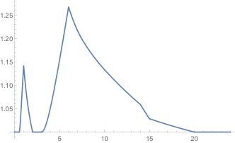
(b) Corresponding PoA

Figure 4. An example where $\operatorname{\mathsf{PoA}}$ goes back to $1$ once at intermediate demands

Fig. 4(a) shows the version where the network is obtained by nesting with two Wheatstone networks. Fig. 4(b) shows the graph of the corresponding PoA. The PoA is equal to $1$ for small demand ($\mu\leq 1/2$), then increases and reaches a local maximum, then it decreases back to $1$ and it remains equal to $1$ for the entire interval $[2,3]$ of demand, then reaches its maximum and, after that, decreases back to $1$, where it remains indefinitely.

Below we list the paths in the network in Fig. 4(a):

$$p_{1}= ~{}O\rightarrow v_{1}\rightarrow D,$$

$$p_{2}= ~{}O\rightarrow v_{4}\rightarrow D,$$

$$p_{3}= ~{}O\rightarrow v_{1}\rightarrow v_{2}\rightarrow v_{4}\rightarrow D,$$

$$p_{4}= ~{}O\rightarrow v_{1}\rightarrow v_{3}\rightarrow v_{4}\rightarrow D,$$

$$p_{5}= ~{}O\rightarrow v_{1}\rightarrow v_{2}\rightarrow v_{3}\rightarrow v_{4}\rightarrow D.$$

The equilibrium flow for $\mu\in[0,+\infty)$ is given explicitly in the following table:

Interval	Cost $\lambda(\mu)$	$p_{1}$	$p_{2}$	$p_{3}$	$p_{4}$	$p_{5}$
$\mu\in[0,1)$	$4\mu$	0	0	0	0	$\mu$
$\mu\in[1,2)$	$2+2\mu$	0	0	$\mu-1$	$\mu-1$	$2-\mu$
$\mu\in[2,6)$	$\displaystyle 1+\frac{5}{2}\mu$	0	0	$\displaystyle\frac{\mu}{2}$	$\displaystyle\frac{\mu}{2}$	0
$\mu\in[6,14)$	$\displaystyle\frac{29}{2}+\frac{\mu}{4}$	$\displaystyle\frac{3}{4}\mu-\frac{9}{2}$	$\displaystyle\frac{3}{4}\mu-\frac{9}{2}$	$\displaystyle\frac{9}{2}-\frac{\mu}{4}$	$\displaystyle\frac{9}{2}-\frac{\mu}{4}$	0
$\mu\in[14,15)$	$18$	$\mu-8$	$\mu-8$	$15-\mu$	$15-\mu$	$\mu-14$
$\mu\in[15,20)$	$\displaystyle 12+\frac{2}{5}\mu$	$\displaystyle\frac{3}{5}\mu-2$	$\displaystyle\frac{3}{5}\mu-2$	0	0	$\displaystyle 4-\frac{\mu}{5}$
$\mu\geq 20$	$\displaystyle 10+\frac{\mu}{2}$	$\displaystyle\frac{\mu}{2}$	$\displaystyle\frac{\mu}{2}$	0	0	0

As a consequence, the PoA is

$$\operatorname{\mathsf{PoA}}(\mu)=\begin{cases}1&\text{if }\mu\in[0,\frac{1}{2})\\ \dfrac{8\mu^{2}}{-1+4\mu+4\mu^{2}}&\text{if }\mu\in[\frac{1}{2},1)\\[10.0pt] \dfrac{4+4\mu}{2+5\mu}&\text{if }\mu\in[1,2)\\[10.0pt] 1&\text{if }\mu\in[2,3)\\[10.0pt] \dfrac{4\mu+10\mu^{2}}{-81+58\mu+\mu^{2}}&\text{if }\mu\in[3,6)\\[10.0pt] \dfrac{58\mu+\mu^{2}}{-81+58\mu+\mu^{2}}&\text{if }\mu\in[6,7)\\[10.0pt] \dfrac{58\mu+\mu^{2}}{-130+72\mu}&\text{if }\mu\in[7,\frac{15}{2})\\[10.0pt] \dfrac{290\mu+5\mu^{2}}{-200+240\mu+8\mu^{2}}&\text{if }\mu\in[\frac{15}{2},10)\\[10.0pt] \dfrac{58+\mu}{40+2\mu}&\text{if }\mu\in[10,14)\\[10.0pt] \dfrac{36}{20+\mu}&\text{if }\mu\in[14,15)\\[10.0pt] \dfrac{120+4\mu}{100+5\mu}&\text{if }\mu\in[15,20)\\[10.0pt] 1&\text{if }\mu\geq 20.\end{cases}$$ (5.1)

The case of three nested Wheatstone networks can be treated similarly (see Fig. 5). Here the PoA is $1$ in the intervals $[0,\frac{1}{2}]$, $[2,3]$, $[20,30]$ and $[200,+\infty)$.

(a) Three nested Wheatstone networks

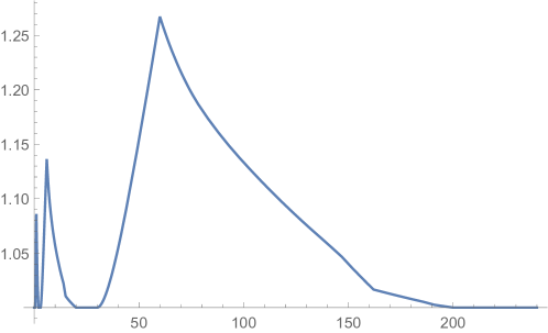
(b) Corresponding PoA

Figure 5. An example where $\operatorname{\mathsf{PoA}}$ goes back to $1$ twice at intermediate demands

Example 5.4.

This example shows that the result in Theorem 4.4 fails for polynomials, even for the simplest network topology. Indeed, consider the two-link parallel network with cost functions

$$\begin{split}c_{1}(x_{1})&=x_{1},\\ c_{2}(x_{2})&=1+x_{2}^{2}.\end{split}$$ (5.2)

The equilibrium and optimum flows can be computed explicitly as:

demand	$x^{\ast}_{1}(\mu)$	$x^{\ast}_{2}(\mu)$	$\widetilde{x}_{1}(\mu)$	$\widetilde{x}_{2}(\mu)$
$\mu\in[0,1/2]$	$\mu$	0	$\mu$	0
$\mu\in[1/2,1]$	$\mu$	0	$\mu-\dfrac{-1+\sqrt{6\mu-2}}{3}$	$\dfrac{-1+\sqrt{6\mu-2}}{3}$
$\mu\in[1,+\infty)$	$\mu-\dfrac{-1+\sqrt{4\mu-3}}{2}$	$\dfrac{-1+\sqrt{4\mu-3}}{2}$	$\mu-\dfrac{-1+\sqrt{6\mu-2}}{3}$	$\dfrac{-1+\sqrt{6\mu-2}}{3}$

Note that the sole $\widehat{\mathcal{E}}$-breakpoint is at $\mu=1$. Moreover we have $x^{\ast}_{1}(3)=\widetilde{x}_{1}(3)=2$ and $x^{\ast}_{2}(3)=\widetilde{x}_{2}(3)=1$ so that the equilibrium and optimal flows coincide, and $\operatorname{\mathsf{PoA}}(3)=1$. This implies that in the interval $(3,+\infty)$ the PoA has a local maximum (see Fig. 6).

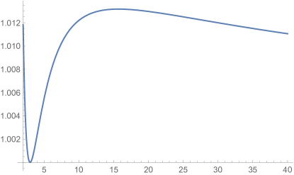
Figure 6. Plot of the PoA on the interval $[2,40]$ for the parallel network with costs as in Eq. 5.2.

When the cost functions are less regular, the set of paths used at equilibrium can have a recurring behavior, and an active network that is abandoned at some point can be reactivated at larger demands. In particular we cannot ensure that the number of $\widehat{\mathcal{E}}$-breakpoints is finite.

Proposition 5.1.

There exist networks and nondecreasing cost functions $c_{e}(\,\cdot\,)$ such that a given active network $\widehat{\mathcal{E}}(\mu)=\mathcal{E}_{0}$ can repeat itself over disjoint demand intervals defined by $\widehat{\mathcal{E}}$-breakpoints.

Proof.

Consider the network in Fig. 7 with the cost $c(x)$ defined in $[0,\zeta]\cup[\zeta+\eta,+\infty]$ as follows

$$c(x)=\begin{cases}a&\text{ if }x\leq\zeta\\ b&\text{ if }x\geq\zeta+\eta,\end{cases}$$

with $0<\eta<a<\zeta<\zeta+\eta<b$, and in the interval $[\zeta,\zeta+\eta]$ we interpolate in any way that makes $c(x)$ continuous and nondecreasing in the whole $[0,+\infty]$.

Figure 7. Wheatsone network with nonaffine costs.

Then we have the following regimes:

1. when $\mu\in[0,a]$, the equilibrium flow uses only the path $\{O,v_{1},v_{2},D\}$, the load on the two edges $\{O,v_{2}\}$, and $\{v_{1},D\}$ is zero and the equilibrium cost is $\lambda(\mu)=2\mu$;

2. when $\mu\in(a,2a)$, the equilibrium flow uses all the three paths with the following distribution

   path	$\{O,v_{1},v_{2},D\}$	$\{O,v_{1},D\}$	$\{O,v_{2},D\}$
   flow	$2a-\mu$	$\mu-a$	$\mu-a$

   the load on the two edges $\{O,v_{2}\}$, $\{v_{1},D\}$ is $\mu-a<\zeta$, and the equilibrium cost is $\lambda(\mu)=2a$;

3. when $\mu\in[2a,2\zeta]$, the equilibrium flow splits equally between the two paths $\{O,v_{1},D\}$, $\{O,v_{2},D\}$, the load on the two edges $\{O,v_{2}\}$, $\{v_{1},D\}$ is $\mu/2\leq\zeta$, and the equilibrium cost is $\lambda(\mu)=a+\mu/2$;

4. the regime on the demand interval $[2\zeta,b+\zeta+\eta]$ is complicated to describe, but this is not relevant for our purpose;

5. when $\mu\in[b+\zeta+\eta,2b)$, the equilibrium uses all three paths with the following distribution

   path	$\{O,v_{1},v_{2},D\}$	$\{O,v_{1},D\}$	$\{O,v_{2},D\}$
   flow	$2b-\mu$	$\mu-b$	$\mu-b$

   the load on the two edges $\{O,v_{2}\}$, $\{v_{1},D\}$ is $\mu-b\geq\zeta+\eta$, and the equilibrium cost is $\lambda(\mu)=2b$;

6. when $\mu\geq 2b$, the equilibrium flow splits equally between the two paths $\{O,v_{1},D\}$, $\{O,v_{2},D\}$, and the load on the two edges $\{O,v_{2}\}$, $\{v_{1},D\}$ is $\mu/2>\zeta+\eta$.

This proves our claim, as in the intervals sub c and f the equilibrium uses only the two paths $\{O,v_{1},D\}$ and $\{O,v_{2},D\}$, while in the interval sub b and e it uses all three paths. ∎

Remark 5.1.

Note that in the same way one can construct examples of networks with an infinite number of $\widehat{\mathcal{E}}$-breakpoints for the equilibrium. Furthermore, one can make the increasing sequence of such $\widehat{\mathcal{E}}$-breakpoints to be convergent. Indeed, one could chose infinite sequences $(\eta_{i})_{i\in\mathbb{N}}$, $(a_{i})_{i\in\mathbb{N}}$, $(\zeta_{i})_{i\in\mathbb{N}}$, $(b_{i})_{i\in\mathbb{N}}$ with

$$0<\eta_{i}<a_{i}<\zeta_{i}<\zeta_{i}+\eta_{i}<b_{i}<a_{i+1}\quad\text{for every }i\in\mathbb{N}.$$ (5.3)

Then we set the cost function $c(x)$ to be

$$c(x)=\begin{cases}a_{1}&\text{ if }x\leq\zeta_{1}\\ b_{i}&\text{ if }\zeta_{i}+\eta_{i}\leq x\leq\dfrac{a_{i+1}-b_{i}}{2}\\ a_{i+1}&\text{ if }a_{i+1}\leq x\leq\zeta_{i+1},\end{cases}$$

and in the intervals $[\zeta_{i},\zeta_{i}+\eta]$, $[(a_{i+1}-b_{i})/2,a_{i+1}]$ we interpolate in any way that makes $c(x)$ continuous and nondecreasing in the whole $[0,+\infty]$. With this choice of $c(x)$, the situation is similar to the one of Proposition 5.1, repeated infinitely many times. Furthermore, since the $\eta_{i}$ can be as small as we want, we can choose the sequences $(a_{i})_{i\in\mathbb{N}}$, $(\zeta_{i})_{i\in\mathbb{N}}$, $(b_{i})_{i\in\mathbb{N}}$ to be convergent to the same limit.

Remark 5.2.

Repetition of an active network can happen for cost functions that are smooth or piecewise affine, as in Klimm and Warode, (2021). We know that this cannot happen for affine cost functions, but, so far we have not been able to characterize the class of cost functions for which repetitions of active networks are impossible.

Acknowledgments

Marco Scarsini and Valerio Dose are members of INdAM-GNAMPA. Roberto Cominetti gratefully acknowledges the support of Luiss University during a visit in which this research was initiated, as well as the support of Proyecto Anillo ANID/PIA/ACT192094. This research project received partial support from the COST action GAMENET, the INdAM-GNAMPA Project 2020 Random Walks on Random Games, and the Italian MIUR PRIN 2017 Project ALGADIMAR Algorithms, Games, and Digital Markets.

The authors thank the reviewers for their careful reading of the paper, for their useful suggestions, and for bringing to their attention the article by Klimm and Warode, (2021).

6. List of symbols

$a_{e}$	coefficient of the monomial in an affine cost function
$A$	$Z^{\top}\Gamma Z$, defined in Eq. 4.7
$b_{e}$	constant in an affine cost function
$\boldsymbol{b}$	$(b_{1},\dots,b_{m})^{\top}$
$c_{e}$	cost of edge $e$
$\boldsymbol{c}$	$(c_{1},\dots,c_{m})^{\top}$
$\widetilde{c}_{e}(x_{e})$	$\widetilde{C}_{e}^{\prime}(x_{e})$, defined in Eq. 3.4
$C_{e}$	primitive of $c_{e}$, defined in Eq. 2.5
$\widetilde{C}_{e}(x_{e})$	$x_{e}\,c_{e}(x_{e})$
$c_{p}$	cost of path $p$, defined in Eq. 2.2
$\boldsymbol{d}$	$Z^{\top}\boldsymbol{b}$, defined in Eq. 4.7
$D$	destination of the network
$\mathsf{D}_{\mu}$	dual problem
$e$	edge
$\mathcal{E}$	set of edges
$\widehat{\mathcal{E}}(\mu)$	active network at demand $\mu$, defined in Definition 3.4
$\widehat{\mathcal{E}}_{0}$	$\widehat{\mathcal{E}}(\mu_{0})$
$\mathcal{E}\left(v,w\right)$	set of all edges $e\in\mathcal{E}$ that go from $v$ to $w$
$\widehat{\mathcal{E}}_{0}\left(v,w\right)$	set of all edges $e\in\widehat{\mathcal{E}}_{0}$ that go from $v$ to $w$
$\boldsymbol{f}$	flow profile
$\boldsymbol{f}^{\ast}$	equilibrium flow profile
$\widetilde{\boldsymbol{f}}$	optimum flow profile
$f_{p}$	flow of path $p$
$\mathcal{F}_{\mu}$	set of flows of total demand $\mu$, defined in Eq. 2.1
$\mathcal{G}$	graph
$m$	$\operatorname{card}(\mathcal{E})$
$n$	$\operatorname{card}(\mathcal{P})$
$\mathcal{N^{+}}(v)$	out-edges of vertex $v$
$\mathcal{N^{-}}(v)$	in-edges of vertex $v$
$O$	origin of the network
$p$	path
$\mathcal{P}$	set of paths
$\mathsf{P}_{\mu}$	primal problem
$\operatorname{\mathsf{PoA}}$	price of anarchy
$\mathsf{S}$	solution set
$\operatorname{\mathsf{SC}}$	social cost, defined in Eq. 2.8
$s_{e}$	increment of $\tau_{e}$, defined in the proof of Proposition 3.7
$T_{v}$	equilibrium cost of shortest path to $v$, defined in Eq. 3.10
$u_{e}$	increment of $x_{e}$, defined in the proof of Proposition 3.7
$\mathcal{V}$	set of vertices
$\mathcal{V}_{0}$	set of vertices in the active network
$v_{\mu}(z)$	$\inf_{f}\varphi_{\mu}(\boldsymbol{f},z)$, defined in Eq. 3.2
$V(\mu)$	solution of the equilibrium minimization problem, defined in Eq. 2.4
$\widetilde{V}(\mu)$	solution of the optimum minimization problem, defined in Eq. 2.10
$\boldsymbol{x}$	load profile
$\boldsymbol{x}^{\ast}$	equilibrium load profile
$x_{e}$	load of edge $e$
$\mathcal{X}_{\mu}$	set of loads of total demand $\mu$
$Z$	edge-path incidence matrix
$\alpha$	element of $\mathbb{R}_{+}$, first used in Proposition 4.2
$\alpha_{k}$	element of $\mathbb{R}_{+}$, first used in Proposition 4.3
$\beta$	element of $\mathbb{R}_{+}$, first used in Proposition 4.2
$\beta_{k}$	element of $\mathbb{R}_{+}$, first used in Proposition 4.3
$\gamma$	element of $\mathbb{R}_{-}$, first used in Theorem 4.4
$\gamma_{k}$	element of $\mathbb{R}_{-}$, first used in Proposition 4.3
$\Gamma$	$\operatorname{diag}[(a_{e})_{e\in\mathcal{E}}]$
$\delta$	element of $\mathbb{R}_{+}$, first used in Theorem 4.4
$\delta_{v}$	increment of $T_{v}$, defined in the proof of Proposition 3.7
$\Delta_{v,w}$	constant travel time from $v$ to $w$
$\zeta$	element of $\mathbb{R}_{+}$, first used in the proof of Proposition 5.1
$\eta$	element of $\mathbb{R}_{+}$, first used in Theorem 4.4
$\lambda$	equilibrium cost, defined in Eq. 2.3
$\mu$	demand
$\mu_{0}$	$\widehat{\mathcal{E}}$-breakpoint for the equilibrium, defined in Definition 3.4
$\widetilde{\mu}_{0}$	$\widehat{\mathcal{E}}$-breakpoint for the optimum
$\tau_{e}$	equilibrium cost of edge $e$
$\varphi_{\mu}$	perturbation function, defined in Eq. 3.1

References

- Aliprantis and Border, (2006) Aliprantis, C. D. and Border, K. C. (2006). Infinite Dimensional Analysis. Springer, Berlin, third edition.
- Beckmann et al., (1956) Beckmann, M. J., McGuire, C., and Winsten, C. B. (1956). Studies in the Economics of Transportation. Yale University Press, New Haven, CT.
- Colini-Baldeschi et al., (2020) Colini-Baldeschi, R., Cominetti, R., Mertikopolous, P., and Scarsini, M. (2020). When is selfish routing bad? The price of anarchy in light and heavy traffic. Oper. Res., 68(2):411–434.
- Colini-Baldeschi et al., (2019) Colini-Baldeschi, R., Cominetti, R., and Scarsini, M. (2019). Price of anarchy for highly congested routing games in parallel networks. Theory Comput. Syst., 63(1):90–113.
- Colini-Baldeschi et al., (2018) Colini-Baldeschi, R., Klimm, M., and Scarsini, M. (2018). Demand-independent optimal tolls. In 45th International Colloquium on Automata, Languages, and Programming. Schloss Dagstuhl. Leibniz-Zent. Inform., Wadern.
- Cominetti et al., (2019) Cominetti, R., Scarsini, M., Schröder, M., and Stier-Moses, N. (2019). Price of anarchy in stochastic atomic congestion games with affine costs. In Proceedings of The Twentieth ACM Conference on Economics and Computation (ACM EC ’19).
- Correa et al., (2004) Correa, J. R., Schulz, A. S., and Stier-Moses, N. E. (2004). Selfish routing in capacitated networks. Math. Oper. Res., 29(4):961–976.
- Correa et al., (2007) Correa, J. R., Schulz, A. S., and Stier-Moses, N. E. (2007). Fast, fair, and efficient flows in networks. Oper. Res., 55(2):215–225.
- Correa et al., (2008) Correa, J. R., Schulz, A. S., and Stier-Moses, N. E. (2008). A geometric approach to the price of anarchy in nonatomic congestion games. Games Econom. Behav., 64(2):457–469.
- Correa and Stier-Moses, (2011) Correa, J. R. and Stier-Moses, N. E. (2011). Wardrop equilibria. In Cochran, J. J., editor, Encyclopedia of Operations Research and Management Science. Wiley.
- Dafermos and Nagurney, (1984) Dafermos, S. and Nagurney, A. (1984). Sensitivity analysis for the asymmetric network equilibrium problem. Math. Programming, 28(2):174–184.
- Dafermos and Sparrow, (1969) Dafermos, S. C. and Sparrow, F. T. (1969). The traffic assignment problem for a general network. J. Res. Nat. Bur. Standards Sect. B, 73B:91–118.
- Dumrauf and Gairing, (2006) Dumrauf, D. and Gairing, M. (2006). Price of anarchy for polynomial Wardrop games. In WINE ’06: Proceedings of the 2nd Conference on Web and Internet Economics, pages 319–330. Springer Berlin Heidelberg, Berlin, Heidelberg.
- Englert et al., (2010) Englert, M., Franke, T., and Olbrich, L. (2010). Sensitivity of Wardrop equilibria. Theory Comput. Syst., 47(1):3–14.
- Fisk, (1979) Fisk, C. (1979). More paradoxes in the equilibrium assignment problem. Transportation Res. Part B, 13(4):305 – 309.
- Florian and Hearn, (1995) Florian, M. and Hearn, D. (1995). Network equilibrium models and algorithms. In et al, M. H., editor, Handbooks in Operation Research and Management Science, volume 8. North Holland, Amsterdam.
- Fukushima, (1984) Fukushima, M. (1984). On the dual approach to the traffic assignment problem. Transportation Res. Part B, 18(3):235–245.
- Gemici et al., (2019) Gemici, K., Koutsoupias, E., Monnot, B., Papadimitriou, C. H., and Piliouras, G. (2019). Wealth inequality and the price of anarchy. In 36th International Symposium on Theoretical Aspects of Computer Science. Schloss Dagstuhl. Leibniz-Zent. Inform., Wadern.
- Hall, (1978) Hall, M. A. (1978). Properties of the equilibrium state in transportation networks. Transportation Sci., 12(3):208–216.
- Josefsson and Patriksson, (2007) Josefsson, M. and Patriksson, M. (2007). Sensitivity analysis of separable traffic equilibrium equilibria with application to bilevel optimization in network design. Transportation Res. Part B, 41(1):4 – 31.
- Klimm and Warode, (2019) Klimm, M. and Warode, P. (2019). Computing all Wardrop equilibria parametrized by the flow demand. In Proceedings of the Thirtieth Annual ACM-SIAM Symposium on Discrete Algorithms, pages 917–934. SIAM, Philadelphia, PA.
- Klimm and Warode, (2021) Klimm, M. and Warode, P. (2021). Parametric computation of minimum-cost flows with piecewise quadratic costs. Math. Oper. Res., forthcoming.
- Koutsoupias and Papadimitriou, (1999) Koutsoupias, E. and Papadimitriou, C. (1999). Worst-case equilibria. In STACS 99 (Trier), volume 1563 of Lecture Notes in Comput. Sci., pages 404–413. Springer, Berlin.
- Milchtaich, (2006) Milchtaich, I. (2006). Network topology and the efficiency of equilibrium. Games Econom. Behav., 57(2):321–346.
- Monnot et al., (2017) Monnot, B., Benita, F., and Piliouras, G. (2017). Routing games in the wild: efficiency, equilibration and regret. In R. Devanur, N. and Lu, P., editors, Web and Internet Economics, pages 340–353, Cham. Springer International Publishing.
- O’Hare et al., (2016) O’Hare, S. J., Connors, R. D., and Watling, D. P. (2016). Mechanisms that govern how the price of anarchy varies with travel demand. Transportation Res. Part B, 84:55–80.
- Papadimitriou, (2001) Papadimitriou, C. (2001). Algorithms, games, and the Internet. In Proceedings of the Thirty-Third Annual ACM Symposium on Theory of Computing, pages 749–753, New York. ACM.
- Patriksson, (2004) Patriksson, M. (2004). Sensitivity analysis of traffic equilibria. Transportation Sci., 38(3):258–281.
- Pigou, (1920) Pigou, A. C. (1920). The Economics of Welfare. Macmillan and Co., London, 1st edition.
- Rockafellar, (1997) Rockafellar, R. T. (1997). Convex Analysis. Princeton Landmarks in Mathematics. Princeton University Press, Princeton, NJ. Reprint of the 1970 original, Princeton Paperbacks.
- Roughgarden, (2003) Roughgarden, T. (2003). The price of anarchy is independent of the network topology. J. Comput. System Sci., 67(2):341–364.
- Roughgarden and Tardos, (2002) Roughgarden, T. and Tardos, E. (2002). How bad is selfish routing? J. ACM, 49(2):236–259.
- Roughgarden and Tardos, (2004) Roughgarden, T. and Tardos, E. (2004). Bounding the inefficiency of equilibria in nonatomic congestion games. Games Econom. Behav., 47(2):389–403.
- Shapiro, (1988) Shapiro, A. (1988). Sensitivity analysis of nonlinear programs and differentiability properties of metric projections. SIAM J. Control Optim., 26(3):628–645.
- Takalloo and Kwon, (2020) Takalloo, M. and Kwon, C. (2020). Sensitivity of Wardrop equilibria: revisited. Optim. Lett., 14(3):781–796.
- Tomlin, (1966) Tomlin, J. A. (1966). Minimum-cost multicommodity network flows. Oper. Res., 14(1):45–51.
- Wardrop, (1952) Wardrop, J. G. (1952). Some theoretical aspects of road traffic research. In Proceedings of the Institute of Civil Engineers, Part II, volume 1, pages 325–378.
- Wu and Möhring, (2020) Wu, Z. and Möhring, R. (2020). A sensitivity analysis for the price of anarchy in non-atomic congestion games. Technical report, arXiv 2007.13979.
- Wu et al., (2021) Wu, Z., Möhring, R. H., Chen, Y., and Xu, D. (2021). Selfishness need not be bad. Operations Research, 69(2):410–435.
- Youn et al., (2008) Youn, H., Gastner, M. T., and Jeong, H. (2008). Price of anarchy in transportation networks: Efficiency and optimality control. Physical Review Letters, 101(12):128701.
- Youn et al., (2009) Youn, H., Gastner, M. T., and Jeong, H. (2009). Erratum: Price of anarchy in transportation networks: Efficiency and optimality control [phys. rev. lett. 101, 128701 (2008)]. Phys. Rev. Lett., 102:049905.