When Cold Radial Migration is Hot: Constraints from Resonant Overlap

Abstract

It is widely accepted that stars in a spiral disk, like the Milky Way’s, can radially migrate on order a scale length over the disk’s lifetime. With the exception of cold torquing, also known as “churning,” processes that contribute to the radial migration of stars are necessarily associated with kinematic heating. Additionally, it is an open question whether or not an episode of cold torquing is kinemically cold over long radial distances. This study uses a suite of analytically based simulations to investigate the dynamical response when stars are subject to cold torquing and are also resonant with an ultraharmonic. Model results demonstrate that these populations are kinematically heated and have RMS changes in orbital angular momentum around corotation that can exceed those of populations that do not experience resonant overlap. Thus, kinematic heating can occur during episodes of cold torquing. In a case study of a Milky Way-like disk with an exponential surface density profile and flat rotation curve, up to 40% of cold torqued stars in the solar cylinder experience resonant overlap. This fraction increases toward the galactic center. To first approximation, the maximum radial excursions from cold torquing depend only on the strength of the spiral pattern and the underlying rotation curve. This work places an upper limit to these excursions to be the distance between the ultraharmonics, otherwise radial migration near corotation can kinematically heat. The diffusion rate for kinematically cold radial migration is thus constrained by limiting the step size in the random walk approximation.

1 Introduction

Transient spiral arms drive a range of dynamical processes of significant importance to the internal, secular evolution of galactic stellar disks (see Sellwood, 2014, and references therein for a review). Many of these processes cause disk stars to shift radial position away from their birth radius over time, as their orbital angular momenta, orbital energies, and eccentricities can be considerably altered. Such changes are often broadly attributed to “radial migration,” a term which does not distinguish between the manner of change to radial position. In fact, most physical processes that induce radial migration necessitate simultaneous changes to both orbital angular momentum and orbital circularity (e.g., Spitzer & Schwarzschild, 1953; Barbanis & Woltjer, 1967; Lynden-Bell & Kalnajs, 1972; Carlberg & Sellwood, 1985). However, one particular process can reorganize orbital angular momentum in the disk and is assumed to never be associated with kinematic heating, hereafter called “ cold torquing.” Cold torquing is the physical mechanism identified by Sellwood & Binney (2002) that drives ‘churning’ of stellar populations. A star can migrate by cold torquing when it is in a stable orbit with the corotation resonance of a transient spiral; the corotation resonance occurs where the circular orbital frequency of stars equals the pattern speed of a spiral (or other) perturbation to the potential.

Present day kinematic, chemical, and structural properties of the stellar disk depend on the amount of kinematic heating produced by all forms of radial migration over time. The degree to which kinematically cold forms of radial migration affect the evolution of disk galaxies is thought to be directly dependent on the efficiency of cold torquing. However, theoretical studies have yet to develop a deep understanding for how kinematically cold radial migration through cold torquing truly is in all circumstances. It is therefore important to reevaluate the assumption that cold torquing is always kinematically cold and, if not, to understand any constraints to that assumption.

In order for cold torquing to be efficient, multiple generations of transient spiral arms with multiple pattern speeds (and thus corotation radii) must occur over a disk’s lifetime. Each episode causes stars to take a single step in a random walk-like redistribution of orbital angular momentum, where the standard deviation in the final distribution of stars for a given birth radius is proportional to the size of a single step. Thus, a limit to the size of a single step in the radial redistribution of stars via cold torquing sets a limit to the final redistribution of stars over the lifetime of the disk.

It is generally accepted that the maximum radial distance a star can migrate via a single episode of cold torquing (Sellwood & Binney, 2002),

$$\Delta R_{\rm max}=2\sqrt{\dfrac{|\Phi_{1}|}{AB}},$$ (1)

depends on the square root of the amplitude of the perturbation to the potential, $\Phi_{1}$, and the Oort constants for sheer and vorticity, $A$ and $B$. The above expression reduces to $\Delta R_{\rm max}\propto\sqrt{|\Phi_{1}|}$ in a disk with a flat rotation curve. Under this assumption, stars can have arbitrarily large changes in their orbital angular momenta with no change to their orbital eccentricity since the amplitude of these changes only depends on the spiral strength.

It has long been accepted that additional patterns exist in the disk, like a bar, and these perturbations each have resonances, like the Lindblad resonances (LRs) and their ultraharmonics. Minchev & Famaey (2010); Minchev et al. (2011) recognized that the radial range for radial migration could be enhanced by overlapping a harmonic of a LR from one pattern with the corotation resonance of another. They found that stellar populations that were subject to this type of resonant overlap had strong signatures of radial migration since the RMS changes in orbital angular momentum in regions of resonant overlap were greater than the expected sum from each resonance, thus suggesting a non-linear, enhanced disk response.

It is usually presumed that a single spiral pattern could not have regions of resonant overlap in the phase-space of a stellar population. However, Daniel & Wyse (2015) showed that the corotation resonance is not defined by a single radius. Rather, corotation is better described by a region in phase-space which can overlap with ultraharmonics from the same pattern. Schaffner et al. (in preparation) used a novel approach, called Permutation Entropy and Statistical Complexity (PESC) (Bandt & Pompe, 2002; Rosso et al., 2007; Weck et al., 2015; Brown et al., 2015; Schaffner et al., 2016), to identify the dynamical response for stars meeting both the corotation and ultraharmonic resonant criteria from a single perturbation to be chaotic.

This paper investigates how the overlap of the corotation region with the inner and outer ultraharmonic resonances of the same perturbation affects disk kinematics. A review of the theory relevant to dynamical resonance in a disk, cold torquing, and resonant overlap is given in §2. The approach is described in §3, including the model used (§3.1), the production of orbits (§3.2), the quantitative characterization of those orbits (§3.3), and the orbital categorization scheme used for analysis (§3.4). This study is limited to the disk response from a single transient spiral pattern, but a discussion on scaling relations for the degree of kinematic heating associated with cold torquing is given in §4. The discussion in §4.1 proposes a reevaluation of the assumption that cold torquing from a single spiral pattern is necessarily a cold process. The discussion §4.2, considers limits to the radial range within which cold torquing is kinematically cold. A brief summary of the conclusions are given in §5.

2 Theoretical Background

The significance of cold torquing, as opposed to other mechanisms for radial migration, is that it is assumed to be kinematically cold. This result arises from the derivation for cold torquing in action space since it conserves the radial action of a star while altering azimuthal action (equal to angular momentum in a disk) (Sellwood & Binney, 2002). For a population of thin disk stars, with orbital eccentricities small enough that the epicyclic approximation holds, this translates to altering orbital sizes without increasing the radial velocity dispersion. Populations of stars that are subject to cold torquing also have, on average, conserved vertical action (Solway et al., 2012) as long as non-axisymmetric perturbations are relatively weak and the affected orbits only mildly eccentric (Vera-Ciro & D’Onghia, 2016).

The impact of cold torquing on disk evolution is different from the impact from forms of radial migration that induce kinematic heating, but, in practice, it is difficult to disentangle the relative importance of each. Large surveys of Milky Way stars have produced significant evidence for radial migration including highly suggestive tracers for past episodes of cold torquing. Radial migration is frequently invoked to explain the degree of increasing spread in the metallicity distribution at a given galactocentric radius with increasing age (e.g., Casagrande et al., 2011; Ness et al., 2016) but the extent to which this can be attributed to cold torquing is unclear. The [Fe/H] distributions from APOGEE (Alam et al., 2015) for stars in the plane of the disk (vertical height $|z|<0.50$ kpc) are skewed with tails toward lower/higher metallicity in the inner/outer disk (Hayden et al., 2015). Such a skew can be understood to arise when stars from the outer/inner disk have significant changes in their orbital angular momentum and thus, assuming a more rapid star formation rate in the inner disk, contaminate stellar populations in the inner/outer disk with lower/higher metallicity stars. Indeed, these skews were fit by a N-body+SPH simulation that resolves radial migration including cold torquing (Loebman et al., 2016). However, a recent model that treats all types of radial migration with a single diffusive prescription is also able to reproduce a similar skew (Frankel et al., 2018). Adding kinematic information can greatly help constrain the role of cold torquing. Perhaps the smoking gun for past cold torquing in the Galaxy comes from the RAVE survey (Steinmetz et al., 2006) with which Kordopatis et al. (2015) identified metal enhanced stars in the solar neighborhood on nearly circular orbits. In fact, the metallicity of the Sun suggests it has migrated from a birth radius that was on order a scale length closer to the galactic center (Wielen et al., 1996; Frankel et al., 2018).

It has been proposed that very efficient cold torquing over the lifetime of the disk could even lead to the emergence of structures like the outer disk (Roškar et al., 2008; Debattista et al., 2017) and the thick disk (Schönrich & Binney, 2009a; Loebman et al., 2011; Schönrich & McMillan, 2017). Attempts to theoretically constrain the past efficiency of cold torquing in the solar neighborhood have had moderate success. A model that included a prescription for cold torquing (Schönrich & Binney, 2009a, b) was able to reproduce solar neighborhood chemistry in the thin disk. However, this model treated cold torquing as a diffusive process that did not depend on the kinematic temperature of the affected population. Daniel & Wyse (2018) used an analytic approach to demonstrate that the fraction of stars that could migrate radially via cold torquing decreases with increasing velocity dispersion. This is in agreement with results from simulations which find preferential cold torquing for populations with smaller velocity dispersion and vertical excursions (Solway et al., 2012; Vera-Ciro et al., 2016). N-body simulations of a quiescent MW-like disk (Aumer et al., 2017) found that the redistribution of angular momentum for stars born in a region corresponding to the Solar neighborhood nearly matched Schönrich & Binney’s prediction. However, while many models and simulations are able to reproduce Solar neighborhood chemistry and kinematics, the explanations are sometimes seemingly contradictory. This likely points to a lack of complete understanding for the dynamical mechanisms driving radial migration.

Analytic scaling relations that can use spiral disk structure to place limits on the impact of cold torquing could assist our interpretation of observational and simulated data.

2.1 Corotation Resonance

A particular family of orbits, sometimes called ‘horseshoe’ orbits, underlie the physics that can lead to cold torquing (Goldreich & Tremaine, 1982; Sellwood & Binney, 2002; Daniel & Wyse, 2015). These orbits occur near the corotation resonance, where the orbital frequency of stars, $\Omega(R)$, equals the pattern speed, $\Omega_{p}$, of a non-axisymmetry in the disk. A star with a trajectory that belongs to this orbital family, hereafter called ‘trapped’, will have periodic changes in orbital angular momentum, $L_{z}$, causing its mean orbital radius, $R_{L}$, to oscillate about the radius of corotation, $R_{\rm CR}$. The mean orbital radius of a star can be defined by using its orbital angular momentum such that,

$$R_{L}=\dfrac{v_{\phi}}{v_{c}}R,$$ (2)

where $v_{c}$ is the orbital circular velocity at $R_{L}$, $v_{\phi}$ is the instantaneous tangential velocity about the disk, and $R$ is the instantaneous radial position of the star. Critical to the definition for cold torquing , there is little to no change in the star’s orbital circularity after a trapped orbital period. Should the non-axisymmetric pattern be transient, a trapped star could have a permanent change in its orbital angular momentum, and thus mean orbital radius, and no change in its orbital circularity (Sellwood & Binney, 2002).

An approximation for the behaviour of a star in a trapped orbit was derived in Section 3.3.3 of Binney & Tremaine (1987) and invoked to describe limits on cold torquing by Sellwood & Binney (2002). This approximation assumes a smooth disk that is perturbed by a weak bar pattern with potential amplitude, $|\Phi_{b}|$, at the radius of corotation. By making the further assumption that the underlying disk has a flat rotation curve, the maximum radial excursion for a star in a trapped orbit scales as $\Delta R\propto\sqrt{|\Phi_{b}|}$, and the minimum time-scale for the smallest excursions scale as $T_{min}\propto R_{\rm CR}/\sqrt{|\Phi_{b}|}$. While these provide guidelines for approximating the efficiency of cold torquing, it may be informative to refine these scaling relations.

Daniel & Wyse (2015) demonstrated that the location of corotation does not occur only at the radius where $\Omega(R)=\Omega_{p}$. Rather corotation can be better described in coordinate space by a 2D region in the plane of the disk. Disk stars with their mean orbital radius within this ‘corotation region’ are, to first order, trapped in stable orbits around corotation. The analytic criterion is derived in action space where vertical action is assumed to be separable in a thin disk. A transformation can be made from 4D action-angle-space to 4D phase-space for a given radially local rotation curve, spiral strength, and pitch angle. A star is trapped when it’s mean orbital radius, $R_{L}$, is approximately within the 2D coordinate-space corotation region, where there is a higher order dependence on orbital circularity. The shape of the corotation region depends on the morphology of the spiral pattern in that the radial range of the corotation region increases with increasing spiral strength and openness of the spiral arms. There is also a dependence on the rate of divergence with radial distance from corotation between the spiral arm’s pattern speed and the orbital frequency for disk stars. For example, spirals that corotate with the disk at all radii ($\Omega(R)=\Omega_{p}(R)$) have the largest corotation regions, possibly spanning the full radius of the disk (Grand et al., 2012; D’Onghia et al., 2013), while a spiral with radially constant pattern speed ($\Omega_{p}=const$) in a Keplerian disk ($\Omega(R)\propto R^{-3/2}$) will have a much less extended corotation region (see equation 32 in Daniel & Wyse, 2015, for their generalized analytic expression for the shape of the corotation region).

2.2 Lindblad Resonances and the Ultraharmonics

The inner and outer Lindblad resonances (ILR/OLR) are where a disk star passes or is passed by the spiral pattern at the star’s epicyclic frequency, $\kappa$. The LRs and their harmonics occur at radii where,

$$\kappa=\pm m\,(n+1)\,[\Omega_{p}-\Omega(R)],$$ (3)

is satisfied, where $n$ stands for the $n^{th}$ harmonic of the Lindblad resonance and $m$ is the number of spiral arms. The inner and outer Lindblad resonances have harmonic number $n=0$ in this notation. In a disk with a flat rotation curve, the radial locations for the LRs are given by,

$$R_{\rm LR}^{(n+1)}=\left(1\mp\dfrac{\sqrt{2}}{m\,(n+1)}\right)\dfrac{v_{c}}{\Omega_{p}},$$ (4)

where $\Omega_{p}=v_{c}/R_{\rm CR}$.

2.3 Resonant Overlap

Higher order harmonics of the LRs ($n>0$) are alone not expected to have a significant impact on disk kinematics. However, since the corotation region has some finite radial range, it is possible for stars in otherwise stable, trapped orbits that have radially periodic orbits about the corotation radius to temporarily also be in resonance with a harmonic of the LRs. Chirikov (1979) predicted that stochastic behaviour emerges in cases where more than one resonance occupies the same N-dimensional space. He drew particular attention to the case of a pendulum under the influence of an external, periodic perturbation; a well known example of chaotic behaviour. Explorations into the kinematic response of a stellar disk in the presence of multiple, non-axisymmetric patterns with different pattern speeds suggest there is a stochastic response for stars at radii that meet a resonant criterion for each pattern (e.g., Quillen, 2003; Jalali, 2008; Minchev & Famaey, 2010).

The nature and degree of the dynamical response to resonant overlap can be challenging to identify. ‘Wild’ (Martinet, 1974) or ergotic (Athanassoula et al., 1983) behaviour associated with resonant overlap can be identified in regions of a surface of section (SoS) diagram by irregularly distributed consequents (see Binney & Tremaine, 2008, §3.7.3). Pichardo et al. (2003) combined SoS and Lyapunov analyses to show that for a sufficiently strong perturbation, orbits in these regions exhibit chaotic behaviour. SoS analysis can have limited utility since, in order to to resolve a chaotic signature, it necessitates a significant number of orbits in order to populate the phase-space within a given energy slice and these are best evolved over several dynamical periods.

In a simultaneous study to the present paper, Schaffner et al. (in preparation) use PESC analysis to effectively investigate the nature of the dynamical response in cases where the corotation region overlaps an ultraharmonic produced by the same perturbation. Since perturbation theory cannot predict non-linear effects from resonant overlap, PESC analysis provides an avenue to identify such a dynamical response. The PESC method is well suited to identifying chaos in poorly resolved or limited data-sets since it does not need to fill the phase-space, it best identifies a chaotic response on shorter, rather than longer, time-scales, and it uses only one governing dimension. In the case of resonant overlap, time-scales from classical perturbation theory do not apply since non-linear affects causing the chaotic response happen on arbitrarily short time-scales. For some of the same models described in this work, Schaffner et al. find a significant chaotic signature using only orbital angular momentum for star particles in small batches of few$\times 10^{2}$ orbits on time-scales less than an orbital period and time-resolution equal to $\sim T_{\rm Dyn}/20$. Figure 1 shows an example of the results using PESC analysis for orbits that are resonant with only corotation (squares, Type 1) and orbits that are resonant with both corotation and an ultraharmonic (circles, Type 3$\rightarrow$2) in model M6e (described below in §3). There are two relevant points. First, there can be a chaotic dynamical response even for a single spiral pattern. Second, that chaotic response is readily quantifiable.

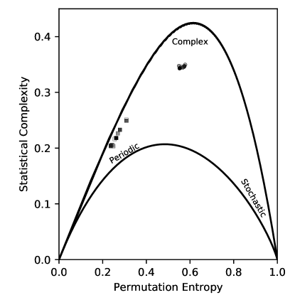
Figure 1: Illustrative example of the bi-modal distribution apparent from PESC analysis for M6e from Schaffner et al. (in preparation) for orbits trapped at corotation that do or don’t have an episode of resonant overlap. Orbits are analyzed over 200 Myr ($0.85\,T_{\rm Dyn}$) using snapshots spaced by 9 Myr ($T_{\rm Dyn}/19$). Orbital analysis is done in groupings of 300 orbits. Shading, from lighter to darker, indicates lower to higher initial orbital angular momentum, respectively. There is no clear trend in the dynamical response within a given orbital type as a function of initial $L_{z}$. Orbits experiencing resonant overlap (circles, Type 3$\rightarrow$2) clearly occupy a region of the PESC diagram that is indicative of complexity or classical chaos, while orbits trapped at corotation only (squares, Type 1) occupy a region that describes periodic orbits. A general overview of the technique and its applications is presented in Weck et al. (2015) and Brown et al. (2015), and a description of the delay variation technique used on a different timeseries dataset is discussed in Schaffner et al. (2016). Complete definitions for the parameters used and methods for the particular example of galactic orbits are deferred to Schaffner et al. (in preparation).

The nature of the dynamical response during resonant overlap is not the aim of the present study. Rather, the focus is on whether or not the disk response due to resonant overlap can place an upper limit on the efficiency of cold torquing. In the case where the corotation region overlaps the $1^{st}$ harmonic of the LR any stochastic or chaotic dynamical response is of interest. The timescale for a response at the ultraharmonic is reasonable since our tracer particle simulations show that a trapped orbital period is on order a few epicyclic periods. Such a response minimally implies that trapped stars with excursions in their mean orbital radii ($|\Delta R_{L}|$) greater than the distance between the $n=1$ harmonic of the LRs,

$$\Delta R^{(2)}_{\rm LR}=\dfrac{\sqrt{2}R_{\rm CR}}{m},$$ (5)

would have a chaotic response. A strong dynamical response at resonant overlap could lead to a change in orbital family from trapped orbits to non-trapped orbital families. A chaotic response is also a likely driver for radial migration that is associated with kinematic heating. Since kinematic heating is not expected to be associated with radial migration around corotation such resonant overlap is of significant interest.

3 Models

Several models are used to explore the dynamical response due to resonant overlap. All models assume a $m=4$ armed spiral pattern in a 2D disk potential that produces a flat rotation curve. Within these potentials a set of orbits is evolved. The method for producing each model’s set of orbital initial conditions is discussed in §3.1. These initial conditions are evolved to produce a trajectory as described in §3.2. Each trajectory is then categorized as described in §3.3-3.4.

3.1 Initial Conditions

Initial conditions for each star particle is produced by sampling the distribution function, $f_{\rm new}$ from Dehnen (1999). This distribution function resembles a kinematically warm 2D disk and has moments that are similar to observed trends in the Milky Way; namely, a flat rotation curve (e.g., Rubin, 1983; Sofue et al., 2009, and references therein) and an exponential surface density profile (e.g., Freeman, 1970; van der Kruit, 1987; Jurić et al., 2008; de Jong et al., 2010). In energy-momentum space this distribution function is given by,

$$f_{\rm new}(E,L_{z})=\dfrac{\Sigma(R_{E})}{\sqrt{2}\pi\sigma_{R}^{2}(R_{E})}\exp\left\{\dfrac{\Omega(R_{E})[L_{z}-L_{c}(R_{E})]}{\sigma_{R}^{2}(R_{E})}\right\},$$ (6)

where $R_{E}$ is the orbital radius for a star in a circular orbit with energy $E$, $\Omega(R)$ is the circular frequency at a given radial coordinate, $L_{z}$ represents orbital angular momentum about the $z$-axis, $L_{c}(R)$ is the orbital angular momentum for a star in a circular orbit at radius $R$, and $\sigma_{R}(R)$ is the radial velocity dispersion at radius $R$.

The Python based galaxy modelling package galpy v1.4 (Bovy, 2015) is used to produce a set of initial conditions for each model. The galpy command dehnendf is set to numerically refine the initial distribution function given by equation 6 over 20 iterations so that the final distribution function better approximates an exponential surface density profile and flat rotation curve (see Bovy, 2015, for more details). This is done by setting $\beta=0$ and niter$=20$. galpy uses natural length unit $h_{0}$ and natural velocity unit is $v_{0}$. Both the radial velocity dispersion profile ($\sigma_{R}(R)$) and the radial surface density profile, $\Sigma(R)$, are assumed to be exponential. The scale length, $h_{\sigma}$, for $\sigma_{R}(R)$ is set to $h_{\sigma}=h_{0}$ and is assumed to be three times the scale length, $h_{R}$, for $\Sigma(R)$. The radial velocity dispersion profile is normalized so that $\sigma_{R}(h_{0})=0.16\,v_{0}$.

The galpy function sample is used to produce initial conditions for a set of test particles in several models. The number of initial conditions, $N$, minimum and maximum sampling radii, $R_{min}$ and $R_{\rm max}$ respectively, for each model are given in Table 1. The radial ranges for the sampling annuli are chosen to span approximately 4 kpc centered on corotation in order to provide a complete sampling of the corotation region with minimal inclusion of initial conditions for stars that are never trapped at the corotation resonance.

4D phase-space coordinates were recovered for each initial condition by setting parameter returnOrbit=True. Each phase-space coordinate is transformed from natural to physical coordinates using $v_{0}=220$ km s^-1 and $h_{0}=8$ kpc.

3.2 Orbital Integration

Each orbital trajectory is calculated from the initial phase-space coordinate using the 2^nd order leapfrog orbital integrator with fixed $\delta t=10^{5}$ yr time-steps initially described in Daniel & Wyse (2015). Orbits are evolved through the potential given by,

$$\Phi(R,\phi,t)=\Phi_{0}(R)+\Phi_{1}(R,\phi,t),$$ (7)

where $\Phi_{0}(R)$ is the radially dependent axisymmetric disk potential and $\Phi_{1}(R,\phi,t)$ is a time-dependent non-axisymmetric spiral perturbation to the underlying potential.

An analytic form for the underlying potential is chosen such that it is approximately consistent with the moments produced by the adopted distribution function ($f_{\rm new}$, equation 6) for a 2D disk, but it is not strictly self-consistent through Poisson’s equation and the collisionless Boltzmann equation. The underlying disk potential is set to,

$$\Phi_{0}(R)=v_{c}^{2}\ln(R/R_{p}),$$ (8)

where the circular velocity is set so that $v_{c}=v_{0}$ and the scale length for the potential is $R_{p}=1$ kpc, in order to reproduce a flat rotation curve in two dimensions. For the sake of analytic simplicity the spiral perturbation to the potential is assumed to be a density wave given by (Lin et al., 1969),

$$\Phi_{1}(R,\phi,t)=\Phi_{s}(R,t)\cos\left[\alpha\ln(R/R_{\rm CR})+m(\Omega_{p}t-\phi)\right],$$ (9)

where $\phi$ is the azimuthal coordinate, and the constant $\alpha=m\cot\theta$ depends on the spiral pitch angle, $\theta$.

The amplitude of the spiral perturbation,

$$\Phi_{s}(R,t)=\dfrac{2\pi GR\Sigma(R)\epsilon(t)}{\alpha},$$ (10)

depends on the radial surface density profile and the time-dependent fractional amplitude of the surface density, $\epsilon(t)$.

The adopted time dependence for $\epsilon(t)$ has the Gaussian form,

$$\epsilon(t)=\epsilon_{0}\,e^{-(t-2T_{\rm Dyn})^{2}/2\sigma_{t}^{2}},$$ (11)

so that the peak spiral amplitude occurs two orbital periods, $2T_{\rm Dyn}$, after the simulation begins, where the standard deviation is set to $\sigma_{t}=T_{\rm Dyn}$. These assumptions ensure slow growth and decay for the perturbation, thus avoiding a non-adiabatic dynamical response. The value for the maximum fractional amplitude is set to $\epsilon_{0}=0.3$.

This study explores two forms for the radial surface density profile for the disk, $\Sigma(R)$. The distribution function, $f_{\rm new}$, produces an exponential surface density profile in a 2D disk which is expressed analytically by,

$$\Sigma(R)=\Sigma_{0}\,e^{-R/R_{d}},$$ (12)

where the disk scale length for the surface density $R_{d}$ is set to match the prescription used for the distribution function $R_{d}=h_{R}=R_{0}/3$.

An alternate set of models uses an inverse radial form for the surface density,

$$\Sigma(R)=\dfrac{\Sigma_{0}}{R}.$$ (13)

This form is self-consistent for the adopted axisymmetric potential, $\Phi_{0}(R)$ (equation 8), but not with the assumed distribution function (equation 6). In all models $\Sigma_{0}$ is set so that the the surface density at $R_{0}$ is 50 M_⊙ pc^-2, similar to conditions in the solar neighbourhood of the Galaxy (e.g. Kuijken & Gilmore, 1991).

Test particle trajectories in each model are evolved for four orbital periods, where $T_{\rm Dyn}$ is given in Table 1.

Each model is named to signify its assumed radius of corotation, $R_{\rm CR}=\{4,5,6,7,8,9,10\}$ kpc, and adopted surface density profile. For example, model M6e assumes $R_{\rm CR}=6$ kpc and an exponential, “e,” surface density profile.

Table 1: Model Parameters

Parameter	M4e & M4i	M5e	M6e & M6i	M7e	M8e & M8i	M9e	M10e & M10i
$N$	25,000	15,000	50,000	25,000	25,000	15,000	25,000
$R_{min}$ ($R_{0}$)	0.300	0.375	0.400	0.625	0.700	0.875	1.000
$R_{\rm max}$ ($R_{0}$)	0.800	0.875	1.000	1.125	1.400	1.375	1.600
Area ($\pi R_{0}^{2}$)	0.550	0.625	0.840	0.875	1.470	1.125	1.560
$R_{\rm CR}$ (kpc)	4	5	6	7	8	9	10
$T_{\rm Dyn}$ (Gyr)	0.11	0.14	0.17	0.20	0.22	0.25	0.28

Note. — Notes – Parameters for orbital initial conditions (top section) are discussed in §3.1. Parameters for orbital integration (bottom section) are discussed in §3.2. The annular area for the initial positions is also given in natural units. Models using an exponential form ($\Sigma\propto e^{-R}$) for the surface density profile have lower-case “e” at the end of the model name and models using an inverse radial form ($\Sigma\propto R^{-1}$) have a lower-case “i.”

3.3 Resonant Trapping at Corotation

Stars in the plane of a non-axisymmetric potential have an invariant energy defined by the Jacobi integral,

$$E_{J}=E-\Omega_{p}L_{z},$$ (14)

where the orbital energy, $E$, and angular momentum about the vertical axis, $L_{z}$, are taken to be in the non-rotating frame. The orbital energy can be defined as,

$$E=E_{c}(R_{L})+E_{\rm ran},$$ (15)

where $E_{c}(R)$ is the orbital energy for a star in a circular orbit with radius $R$ in the unperturbed potential, $R_{L}$ is the radial coordinate in the unperturbed potential for a star in a circular orbit with unit mass angular momentum $L_{z}=R_{L}\,v_{c}$, and $E_{\rm ran}$ is the energy associated with non-circular motions, hereafter called ‘random energy’.

Trapped orbits are stable orbits that are resonant with corotation (see discussion in §2). A star with zero random energy ($E_{\rm ran}=0$) is trapped when the parameter

$$\Lambda_{c}=\dfrac{E_{J}-h_{\rm CR}}{|\Phi_{s}|_{\rm CR}}$$ (16)

has absolute value equal to or less than unity ($-1\leq\Lambda_{c}\leq 1$) (Contopoulos, 1978), where the invariant $h_{\rm CR}$ is the Jacobi integral for a star in a circular orbit at the radius of corotation ($R_{\rm CR}$) in the unperturbed underlying axisymmetric potential. For a star with some finite non-circular energy ($E_{\rm ran}$) to be trapped in a resonant orbit around corotation, the invariant $\Lambda_{c}$ must be replaced with the time-dependent quantity, $\Lambda_{\rm nc}(t)$ (Daniel & Wyse, 2015, their equation 22). For a rotationally supported disk, $v_{\rm ran}/v_{c}\lesssim 0.2$ where $v_{\rm ran}$ is the velocity associated with $E_{\rm ran}$, with a flat rotation curve, the value of $\Lambda_{\rm nc}(t)$ can be expressed as (Daniel & Wyse, 2015, their equation 33),

$$\Lambda_{\rm nc}(t)=\Lambda_{c}-\left(\dfrac{R_{L}(t)}{R_{\rm CR}}\right)\left(\dfrac{E_{\rm ran}(t)}{|\Phi_{s}|_{\rm CR}}\right),$$ (17)

and the criterion for resonant trapping around corotation is satisfied when,

$$-1\leq\Lambda_{\rm nc}(t)\leq 1.$$ (18)

The expression in equation 17 assumes the epicyclic approximation in order to convert from action-space to energy-angular momentum space.

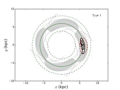
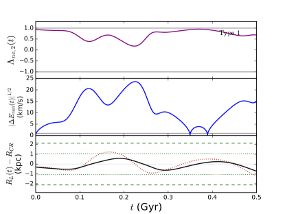
Figure 2: Illustrative example of a stable orbit trapped at the corotation resonance (Type 1). The potential is in Figure 3 for $R_{\rm CR}=6$ kpc. This star particle is launched with initial 4D phase-space coordinates $(x,y,v_{x},v_{y})=(5.7$ kpc, $0$ kpc, $2$ km s^-1, $220$ km s${}^{-1})$ (marked with a black star). The fractional amplitude of the surface density is assumed to be $\epsilon=0.3$ and the pitch angle $\theta=30^{\circ}$. The minima of the $m=4$ spiral pattern are indicated with dashed (magenta) curves. Radius of corotation is shown as a solid (green) curve. Lindblad resonances are shown as long-dashed (green) curves and ultraharmonics are shown as dotted (green) curves. The corotation region is shaded grey. The the left hand panel shows the coordinate trajectory (dashed, red) and the guiding centre radius ($R_{L}$ – solid, black) of the star particle. The right hand panel shows the value for $\Lambda_{\rm nc}(t)$, which satisfies the capture criterion ($|\Lambda_{\rm nc}(t)|\leq 1$) at all times thus indicating it is in a trapped orbit at corotation. The middle right hand panel shows the square root of the absolute value for the change in energy associated with non-circular motions ($|\Delta E_{\rm ran}|^{1/2}$). This trapped orbit has variable circularity, but overall does not experience significant kinematic heating in a single trapped orbital period. The bottom right hand panel shows the mean orbital radius (solid, black) – and radial coordinate (dotted, red) – oscillating about the corotation radius and never meets the ultraharmonic resonance.

Figure 2 shows an example of an orbit that meets the criterion for a stable orbit trapped at the corotation resonance. The left panel shows the trajectory (dashed, red) of the star particle evolved over 0.5 Gyr in a spiral potential with $R_{\rm CR}=6$ kpc. The mean orbital radius ($R_{L}$, equation 4) is indicated by the solid (black) curve and is in the corotation region (shaded) throughout the simulation. The radial coordinate (dotted, red), guiding centre radius (solid, black), their relative distances from the Lindblad resonances (dashed, green), and ultraharmonics (dotted, green) are also shown in the bottom of the right hand panel. Since this is a trapped orbit the mean orbital radius radially oscillates about the corotation radius. The top right hand panel of Figure 2 shows the value for $\Lambda_{\rm nc}(t)$ (equation 17), which satisfies the corotation criterion (equation 18) at all times. The middle right hand panel is square root of the absolute value for the change in energy associated with non-circular motions ($|\Delta E_{\rm ran}|^{1/2}$), which varies throughout the simulation, yet the orbit remains trapped with the corotation resonance.

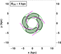
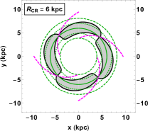
Figure 3: Contours showing the corotation region as a solid, thick (black) curve for models M4e, M6e, M8e, and M10e. Radius of corotation for each model is given in the inset. Line-styles and colors of the curves in both the left hand panel and the bottom right hand panel match the definitions from Figure 2. The degree of resonant overlap depends on the radius of corotation for models assuming spiral amplitude scales with exponential surface density profile.

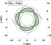
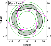
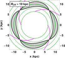
Figure 4: Contours showing the corotation region for models M4i, M6i, M8i, and M10i. Shading and linestyles have same meaning as in Figures 2 & 3. The degree of resonant overlap is nearly constant for models assuming a inverse radial surface density profile illustrating that the expected response for resonant overlap depends on the assumed model.

Figures 3 and 4 show contours for the corotation region in models that use the exponential surface density profile in equation 12 (M4e, M6e, M8e, and M10e) and the inverse radial surface density profile in equation 13 (M4i, M6i, M8i, and M10i) for four different corotation radii. These models were selected in order to illustrate how the distribution of resonances in the disk depends on the radius of corotation and assumed surface density profile when all other parameters are equal. The corotation regions are shaded and outlined by a solid, thick (black) curve, where minima in the spiral potential are shown as short-dashed (magenta) curves. Lindblad resonances are indicated by long-dashed (green) curves, ultraharmonics by dotted (green) curves, and radii of corotation by a solid (green) curves. With decreasing corotation radius, the distances between the Lindblad resonances and ultraharmonics decrease while the area of the corotation region depends on the assumed surface density profile. For models assuming an exponential disk, the corotation region is broader toward the galactic center and therefore trends toward a greater degree of resonant overlap for spiral patterns with a smaller corotation radius (and higher pattern speed). Models adopting the inverse radial surface density profile have radially independent spiral strength and therefore the degree of resonant overlap depends only on the fractional amplitude for the spiral pattern for constant number of arms and pitch angle.

3.4 Orbital categorization Scheme

Table 2: Orbital Categorization Scheme

Category	Description
Type 1	Trapped in resonant orbit about corotation
Type 2	Never trapped at corotation
Type 3$\rightarrow$1	In a trapped orbit before & after crossing
	an ultraharmonic
Type 3$\rightarrow$2	In a trapped before crossing an ultraharmonic,
	but not after
Other	Any other scenario

The expectation for a star trapped at the corotation resonance is that its mean orbital radius ($R_{L}$) will oscillate about corotation ($R_{\rm CR}$) indefinitely with negligible change to its circularity. The primary focus of this work is to critically examine that expectation in cases when a trapped star simultaneously meets another resonant criterion.

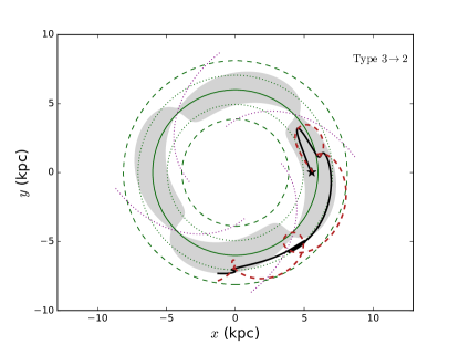
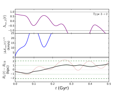
Figure 5: Illustrative example of the orbital response for a star that is initially in a stable orbit trapped at the corotation resonance that later meets a second resonant criterion when the guiding centre radius crosses an ultraharmonic (Type 3). Initial 4D phase-space coordinates for this star are $(x,y,v_{x},v_{y})=(5.6$ kpc, $0$ kpc, $-1$ km s^-1, $218$ km s${}^{-1})$. The line-styles and shading have the same meaning as in Figure 2. Once the star particle crosses the ultraharmonic it is in resonant overlap for nearly 0.25 Gyr. During this time the star particle is kinematically heated, is not trapped as it crosses a spiral arm and then becomes temporarily trapped before ending in a non-resonant orbit (Type 3$\rightarrow$2).

Each test particle’s trajectory is used to calculate a time series array for its orbital angular momentum ($L_{z}$), the associated mean orbital radius ($R_{L}$), the random orbital energy ($E_{\rm ran}$), and $\Lambda_{\rm nc}(t)$. These arrays give a quantitative measure for whether or not a star instantaneously meets any dynamical resonant criteria. A particle is trapped in a resonant orbit about corotation when equation 18 is satisfied via the instantaneous value for $\Lambda_{\rm nc}(t)$ (equation 17). It is resonant with a Lindblad or ultraharmonic resonance when $R_{L}(t)=R_{\rm LR}^{(n+1)}$ (equation 4).

Each of these quantities is calculated using a the time-dependent spiral potential described in §3.2 with the exception of the value for $\Lambda_{\rm nc}(t)$. The value for $\Lambda_{\rm nc}(t)$ is calculated using a time-independent spiral amplitude set to equal the time-dependent potential’s maximum amplitude, $\Phi_{s}(R)=\Phi_{s}(R,2T_{\rm Dyn})$. This choice was made for the following reason. In a potential that includes a transient spiral pattern, all stars begin and end in orbits that are not trapped at corotation since corotation only exists in the presence of a non-axisymmetric perturbation. Using constant $\Phi_{s}(R)$ to evaluate $\Lambda_{\rm nc}(t)$ identifies stars that would remain trapped for the duration of the simulation when the spiral amplitude is large enough for them to be trapped. By adopting this definition, it is possible to distinguish between star particles that are no longer trapped after an episode of resonant overlap from those that are temporarily trapped in Type 1 orbits due to spiral amplitude growth and decay. A comparative study showed that by using a time-dependent spiral potential to calculate $\Lambda_{\rm nc,2}(t)$ there was a small degree of contamination of Type 4 orbits with visually identified Type 1 orbits.

Each trajectory is categorized into one of five types. Star particles that remain in a stable, resonant orbit about corotation for the duration of the simulation are categorized as Type 1. Type 2 orbits are those that never satisfy this criterion and are therefore never in trapped orbits, circulating about the galactic centre in the frame rotating with the spiral pattern for the duration of the simulation. Type 3 orbits begin in trapped orbits and have at least one episode when the mean orbital radius crosses an ultraharmonic, thus simultaneously meeting two dynamical resonant criteria. Type 3 orbits are subdivided into Type 3$\rightarrow$1, which remain in trapped orbits after crossing an ultraharmonic, and Type 3$\rightarrow$2, which are not in trapped orbits at the end of the simulation after crossing an ultraharmonic. All other cases are categorized as ‘Other’. In no case does a trapped orbit have a mean orbital radius that crosses a Lindblad resonance. A summary of these categories is given in Table 2.

Figure 5 shows an illustrative example of a Type 3$\rightarrow$2 orbit, where the star particle does not remain in a trapped orbit after crossing the outer ultraharmonic. In this example, the orbital trajectory is evolved over 0.5 Gyr and begins in a trapped orbit. At $t\sim 0.25$ Gyr, the star particle is in resonance with both corotation ($1\leq|\Lambda_{\rm nc,2}|$) and the outer ultraharmonic ($R_{L}=R^{(2)}_{\rm LR}$) resulting in an increase in non-circular orbital energy ($E_{\rm ran}$). This kinematic heating causes the orbit to no longer be resonant with corotation ($\Lambda_{\rm nc,2}<-1$) and the star particle is therefore able to cross a spiral arm. The star is briefly trapped starting at $t\sim 0.4$ Gyr, but ends in an orbit that is resonant with the outer ultraharmonic only. The orbital response to resonant overlap, being chaotic, is highly variable for very similar initial conditions. In practice, this means that Type 3 orbits commonly have intervals when the orbital trajectory oscillates between being trapped and not trapped with the corotation resonance before being permanently non-trapped. As such, it is likely that the distinction between Type 3$\rightarrow$1 and Type 3$\rightarrow$2 is somewhat unresolved since it is a time-dependent and, given a long enough time-scale, many Type 3$\rightarrow$1 orbits eventually evolve into Type 3$\rightarrow$2 orbits. However, the time-scale for the transient spiral arms in the current simulations ($\sigma_{t}=T_{\rm Dyn}$) is several times less than the time-scale for the simulations ($T=4\,T_{\rm Dyn}$) and so the classifications presented here are expected to be qualitatively robust. We have not accounted for changes to the spiral perturbation’s pattern speed. Analyses of the pattern speeds in simulations with transient spiral arms typically show a time-dependence for spiral pattern speed (e.g., Roškar et al., 2012; D’Onghia et al., 2016). Further exploration is required in order to understand how an evolving pattern speed would affect trapped orbits.

Table 3: Distribution of Orbits for Exponential Surface Density Profile

	M4e	M5e	M6e	M7e	M8e	M9e	M10e
Type 1	842 ($3.4\%$)	862 ($5.8\%$)	3,910 ($7.8\%$)	2,616 ($17.4\%$)	4,782 ($19.1\%$)	4,999 ($33.3\%$)	8,799 ($35.2\%$)
Type 2	12,761 ($51.0\%$)	7,293 ($48.6\%$)	29,179 ($58.4\%$)	6,631 ($44.2\%$)	14,306 ($57.2\%$)	6,861($45.7\%$)	13,080 ($52.3\%$)
Type 3$\rightarrow$1	3,027 ($12.1\%$)	1,794 ($12.0\%$)	4,547 ($9.1\%$)	1,169 ($7.8\%$)	952 ($3.8\%$)	463 ($3.1\%$)	314 ($1.3\%$)
Type 3$\rightarrow$2	4,462 ($17.9\%$)	2,733 ($18.2\%$)	6,357 ($12.7\%$)	2,322 ($15.5\%$)	2,110 ($8.4\%$)	740 ($4.9\%$)	265 ($1.1\%$)
Other	3,908 ($15.6\%$)	2,318 ($15.5\%$)	6,007 ($12.0\%$)	2,262 ($15.1\%$)	2,849 ($11.4\%$)	1,937 ($12.9\%$)	2,542 ($10.2\%$)
Type 3	7,489 ($30.0\%$)	4,527 ($30.2\%$)	10,904 ($21.8\%$)	3,491 ($23.3\%$)	3,062 ($12.3\%$)	1,203 ($8.0\%$)	579 ($2.3\%$)
Type 1+3	8,331 ($33.3\%$)	5,389 ($35.9\%$)	14,814 ($29.6\%$)	6,107 ($40.7\%$)	7,844 ($31.4\%$)	6,202 ($41.4\%$)	9,378 ($37.5\%$)
Type 3$\rightarrow$2/Type 3	$59.6\%$	$60.4\%$	$58.3\%$	$66.5\%$	$68.9\%$	$61.5\%$	$45.8\%$
Type 3/Type 1+3	$89.9\%$	$84.0\%$	$73.6\%$	$57.2\%$	$39.0\%$	$19.4\%$	$6.2\%$
Type 3$\rightarrow$2/Type 1+3	$53.6\%$	$50.7\%$	$42.9\%$	$38.0\%$	$26.9\%$	$11.9\%$	$2.8\%$

Note. — Notes – Number and percentage of trajectories that satisfy the orbital categorization scheme outlined in Table 2 for models that use an exponential surface density profile ($\Sigma(R)\propto e^{-R}$).

The top panel in Table 3 and Table 4 summarizes the distribution of orbits among each of the orbital categories for each model.

The middle panel in each table gives the total the number and percentage of orbits that experience resonant overlap (Type 3) in each simulation as well as the number and percentage of all orbits that have initial conditions for trapped orbits (Type 1+3). The trend in the initial fraction of trapped orbits roughly follows the ratio between the area of the corotation region and the area of the annulus of sampled initial conditions for each model. (Also see Figures 11 & 14d for Model W – and relevant discussion – in Daniel & Wyse, 2018, which show the maximum width for the corotation region and fraction of stars initially in trapped orbits for model parameters equivalent to those in Table 3.)

The bottom panel in each table quantifies several scaling relations that are illustrated in Figure 6. In all models, between  40-80% of trapped stars have an episode of resonant overlap and are not in trapped orbits at the end of the simulation (Type 3$\rightarrow$2/Type 3) as indicated by a dotted (black) line in Figure 6. This suggests that the dynamical response of trapped stars to resonant overlap alters a significant number of orbital classifications from those that lead to well behaved radial migration due to cold torquing to orbits that inhabit other regions of the phase-space and could be kinematically heated. The fraction of the orbits that are initially trapped (Type 3+1) and experience resonant overlap (Type 3) during the total time evolved ($4T_{\rm Dyn}$) is indicated by a solid (red) line (Type 3/Type 3+1). For the series of models that uses an inverse radial surface density profile ($\Sigma\propto R^{-1}$), the radial size of the corotation region closely scales with the distance between the ultraharmonics ($\Delta R_{\rm LR}^{(n+1)}$), so the degree of resonant overlap is nearly constant for these models ($\sim 30\%$). For the series of models that uses an exponential surface density profile ($\Sigma\propto e^{-R}$) the degree of resonant overlap increases toward the galactic center from $\sim 6\%$ for M10e to $\sim 90\%$ for M4e. The shaded (salmon) region shows the ratio of the number of stars initially in trapped orbits that experience resonant overlap and end the simulation in non-trapped orbits to the number of stars that begin in trapped orbits (Type 3$\rightarrow$2/Type 1+3). These trends are similar to those for Type 3/Type 1+3 since the fraction for Type 3$\rightarrow$2/Type 3 is nearly constant.

Table 4: Distribution of Orbits for Inverse Radial Surface Density Profile

	M4i	M6i	M8i	M10i
Type 1	4,598 ($18.4\%$)	8,968 ($17.9\%$)	5,199 ($20.8\%$)	5,062 ($20.3\%$)
Type 2	12,596 ($50.4\%$)	29,074 ($58.2\%$)	14,415 ($57.7\%$)	13,195 ($52.8\%$)
Type 3$\rightarrow$1	1,245 ($5.0\%$)	2,447 ($4.9\%$)	742 ($3.0\%$)	508 ($2.0\%$)
Type 3$\rightarrow$2	782 ($3.1\%$)	2,097 ($4.2\%$)	1,758 ($7.0\%$)	1,934 ($7.7\%$)
Other	5,779 ($23.1\%$)	7,414 ($14.8\%$)	2,886 ($11.5\%$)	4,301 ($17.2\%$)
Type 3	2,027 ($8.1\%$)	4,544 ($9.1\%$)	2,500 ($10.0\%$)	2,442 ($9.8\%$)
Type 1+3	6,625 ($26.5\%$)	13,512 ($27.0\%$)	7,699 ($30.8\%$)	7,504 ($30.0\%$)
Type 3$\rightarrow$2/Type 3	$38.6\%$	$46.2\%$	$70.3\%$	$79.2\%$
Type 3/Type 1+3	$30.6\%$	$33.6\%$	$32.5\%$	$32.5\%$
Type 3$\rightarrow$2/Type 1+3	$11.8\%$	$15.5\%$	$22.8\%$	$25.8\%$

Note. — Notes – Number and percentage of trajectories that satisfy the orbital categorization scheme outlined in Table 2 for models that use the inverse radial surface density profile ($\Sigma(R)\propto R^{-1}$).

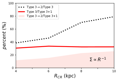
Figure 6: Curves showing the fractional percent for three physically notable orbital classifications. The left plot is for models using an exponential surface density profile ($\Sigma(R)\propto e^{-R}$) to determine spiral strength and the right plot is for models using an inverse radial profile ($\Sigma(R)\propto R^{-1}$). The fraction of trapped orbits that experience resonant overlap with an ultraharmonic is indicated with a solid (red) line (Type 3/Type 3+1). The fraction of those orbits which experience resonant overlap and that are permanently not trapped after crossing an ultraharmonic are indicated with a dotted (black) line (Type 3$\rightarrow$2/Type 3). The shaded (salmon) region shows the fraction of all trapped orbits that are no longer in trapped orbits after an episode of resonant overlap (Type 3$\rightarrow$2/Type 3+1).

4 discussion

It is expected that radial migration of stars as a result of cold torquing leads to a redistribution of orbital angular momentum with no associated kinematic heating (Sellwood & Binney, 2002). The following discussion first suggests a revision to the assumption that cold torquing from a single spiral pattern is necessarily a cold process (§4.1). It then considers limits to the radial range within which cold torquing is kinematically cold (§4.2).

4.1 Kinematic heating from cold torquing

Figures 7 and 8 show the time evolution for the changes in the orbital angular momentum and random orbital energy for populations of star particles in three classification categories. Figure 7 shows models using an exponential surface density profile to determine the spiral amplitude and Figure 8 uses an inverse radial profile. Orbital classifications shown are Type 1 (always trapped – solid, black), Type 3$\rightarrow$1 (resonant overlap occurs, but remain trapped – dashed, orange), and Type 3$\rightarrow$2 (resonant overlap occurs and no longer trapped – dotted, teal). Top panels show RMS changes in orbital angular momentum, $\langle(\Delta L_{z})^{2}\rangle^{1/2}$, using mean orbital radius, $R_{L}$, as a proxy. Horizontal lines indicate half the distance between ultraharmonics as expressed in equation 5. Bottom panels quantify kinematic heating as the square root of the absolute value of the sum of the changes in random orbital energy, $|\Delta E_{\rm ran}|^{1/2}$, so that these changes are expressed in units of velocity. Time is expressed in units of orbital periods, $T_{\rm Dyn}$, where the vertical grey line indicates the moment of peak spiral amplitude.

Trapped orbits (Type 1) have an increase in $\langle(\Delta L_{z})^{2}\rangle^{1/2}$  over time and with increasing spiral amplitude in each model. In most cases, the maximum value for $\langle(\Delta L_{z})^{2}\rangle^{1/2}$ occurs nearly concurrently with the peak spiral amplitude (vertical, grey line). One exception is the offset of this peak for Type 1 (always trapped) orbits, which likely reflects a time-scale difference between the imposed spiral lifetime governed by $\sigma_{t}$ (equation 11) in these simulations and the time-scale for self-gravitational transient spiral structure. Cold torquing likely plays a role in the self-regulation of transient spiral amplitude (Sellwood & Binney, 2002). Further, the time-scale for the radial oscillations of a trapped orbit depends on the maximum radial excursion for that orbit. For a population of trapped stars, the peak in $\langle(\Delta L_{z})^{2}\rangle^{1/2}$ likely occurs on the time-scale that maximizes the phase mixing of trapped orbits, where that time-scale changes with the artificially imposed spiral growth. Relevant to this study is the amplitude of the peak in $\langle(\Delta L_{z})^{2}\rangle^{1/2}$, which is robust whether or not the spiral lifetime is artificially imposed.

The degree of kinematic heating for trapped orbits is not negligible, but is relatively insignificant when compared to other orbital classifications. The low grade heating of Type 1 orbits likely arises from a combination of factors including interactions with spiral arms away from corotation and near passes with the ultraharmonics without crossing. Type 1 orbits experience the greatest degree of heating in models with corotation closer to the inner disk when the surface density profile is exponential. This same demographic describes models with a greater degree of resonant overlap and, therefore, correlates with the fraction of Type 1 orbits that have near encounters with an ultraharmonic.

Trapped orbits that experience resonant overlap (Type 3) also have a rise in $\langle(\Delta L_{z})^{2}\rangle^{1/2}$, but these changes are associated with kinematic heating. In all cases, orbits that are not trapped after experiencing resonant overlap (Type 3$\rightarrow$2) have larger changes in both $\langle(\Delta L_{z})^{2}\rangle^{1/2}$ and $|\Delta E_{\rm ran}|^{1/2}$ than those orbits which remain in trapped orbits (Type 3$\rightarrow$1). Nonetheless, trapped orbits that experience resonant overlap are kinematically heated regardless of whether or not they remain in trapped orbits. With the exception of M10e, Type 3 orbits have larger $\langle(\Delta L_{z})^{2}\rangle^{1/2}$ by the end of the simulation than their Type 1 counterparts. The outstanding case of M10e is likely to do with the very small fraction of Type 3 orbits (2.3%).

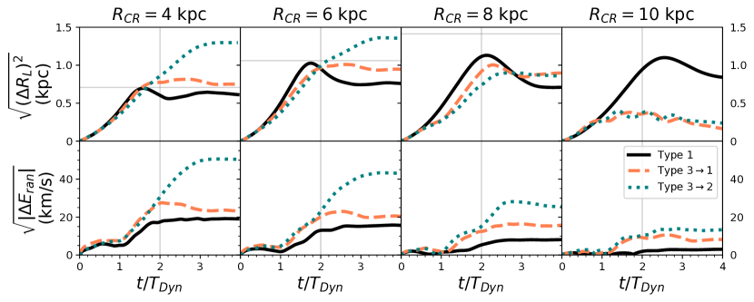
Figure 7: Time evolution of the orbital angular momentum and random orbital energy for populations of star particles in three classification categories. These models use an exponential surface density profile ($\Sigma(R)\propto e^{-R}$) to determine the spiral amplitude. Orbital classifications shown are Type 1 (always trapped – solid, black), Type 3$\rightarrow$1 (resonant overlap occurs, but remain trapped – dashed, orange), and Type 3$\rightarrow$2 (resonant overlap occurs and no longer trapped – dotted, teal). Top panels show RMS changes in orbital angular momentum using mean orbital radius, $R_{L}$ as a proxy, $\langle(\Delta L_{z})^{2}\rangle^{1/2}$, where the horizontal lines indicate half the distance between ultraharmonics. Bottom panels show kinematic heating expressed in velocity units by using $|\Delta E_{\rm ran}|^{1/2}$. Time is expressed in units of orbital periods, $T_{\rm Dyn}$, where the vertical grey line indicates the moment of peak spiral amplitude.

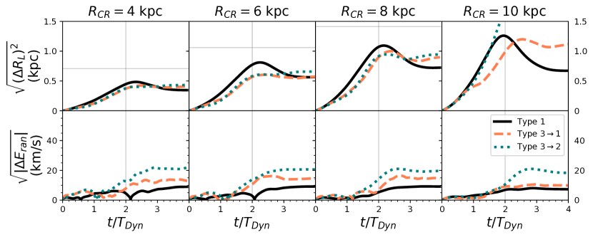
Figure 8: Plots and curves have the same meaning as in Figure 7, where this figure is for models that use an inverse radial surface density profile ($\Sigma(R)\propto R^{-1}$) to determine the spiral amplitude.

4.2 Constraints on radial excursions

The large fraction of orbits that are not trapped after an episode of resonant overlap (Type 3$\rightarrow$2/Type 3) suggests that this dynamical response could be important to understand how disks evolve around corotation. The distance between ultraharmonics increases with increasing radius of corotation and decreasing number of spiral arms (equation 5). This study is limited to spirals with $m=4$ symmetry and so explores the consequence of the spacing between the ultraharmonics as a function of radius of corotation only.

Radial migration from a single episode of cold torquing depends on the radial range of the corotation region (Daniel & Wyse, 2015), which scales with the strength of the spiral perturbation (Sellwood & Binney, 2002). The corotation region is radially more broad toward the galactic center for spirals of the same fractional amplitude of exponential surface density profile. In models that use an inverse radial surface density profile, the radial range for the corotation region closely follows the trend in the radial distance between ultraharmonics. The following discussion does not argue a preference for an underlying model. Rather, it explores the role resonant overlap has on limiting the radial extent of cold radial migration from cold torquing.

Figures 3 and 4 illustrate how the difference between these two models for spiral amplitude affect the fraction of the corotation region that overlaps with the ultraharmonics. The horizontal lines in figures 7 and 8 show the distance between the corotation radius and an ultraharmonic (solid, gray). The curves for $\langle(\Delta L_{z})^{2}\rangle^{1/2}$ for Type 1 orbits never exceed $\Delta R^{(2)}_{\rm LR}/2$ (equation 5) even when the radial range for the corotation region is greater than the annular range between the ultraharmonics. There is therefore a limit to the RMS change in orbital angular momentum, and thus radial changes, for a population of stars migrating from cold torquing that is set by the spacing between ultraharmonics. The spacing between ultraharmonics is more restrictive toward the galactic center. The linear approximation that maximum changes in orbital angular momentum from cold torquing are set by spiral strength must be further constrained by the non-linear response at resonant overlap.

Trapped orbits that experience resonant overlap but remain trapped (Type 3$\rightarrow$1) are also limited by the constraint that $\langle(\Delta L_{z})^{2}\rangle^{1/2}$$\,\leq\Delta R^{(2)}_{\rm LR}/2$. However, orbits that begin trapped at corotation but end in non-trapped orbits after an episode of resonant overlap (Type 3$\rightarrow$2) can have changes in orbital angular momentum that exceed this limit. The implication is that strong transient perturbations can induce large changes in $\langle(\Delta L_{z})^{2}\rangle^{1/2}$, but these changes could be dominated by a large fraction of stars that are kinematically heated due to resonant overlap, even when their changes in orbital angular momentum are around corotation.

It is worth considering that the trends shown in Figure 6 include regions at lower galactocentric radii where, in the Milky Way, the kinematics would be dominated by the bar. Assuming a circular velocity of 220 km s^-1 and bar pattern speed $41\pm 3$ km s^-1 kpc^-1 (Bovy et al., 2019), the Milky Way’s bar has corotation radius equal to $\sim 5.4$ kpc (see also Wegg et al., 2015; Portail et al., 2017). The shape of the underlying potential, and resulting shape of the corotation region, for a bar is rather different from the case of a spiral pattern. Additionally, the vertical component cannot be taken to be separable as can be done with a spiral in a thin disk and as is assumed in the formulation of the capture criterion (Daniel & Wyse, 2015). Nonetheless, there is a significant degree of resonant overlap between the ultraharmonics and the corotation region for a bar. The regions around the L4 and L5 points, which are at the corotation radius and coincident with the azimuthal line through the bar’s minor axis, are typically considered stable. However, in a given barred disk there may be additional resonances between the galactic center and the corotation radius of the bar. In this scenario orbits that would be considered stable in the approximation that corotation is at a particular radius would be subject to resonant overlap when recognizing that the corotation resonance fills some volume in phase-space. Such resonant overlap would presumably induce a chaotic response, where chaotic regions in phase-space are expected to be depopulated (Pfenniger, 1990). Indeed, Buta (2017) uses the evacuation of orbits in these regions in the so called ‘gap method’ to infer the location of corotation and thus other resonances of the bar. These dynamics are currently under further investigation. This discussion is relevant in the current study only insofar as to recognize that the kinematic trend does not reflect the kinematics from resonant overlap from a bar.

5 Conclusions

Cold torquing is a resonant effect that happens around the radius of corotation with a transient spiral pattern. A critical underlying assumption for radial migration by cold torquing is that each transient spiral rearranges orbital angular momentum around corotation without causing kinematic heating. Multiple generations of transient spirals with a range of pattern speeds could cause stellar mean orbital radii to radially diffuse from their birth place in a random walk-like fashion. The standard deviation for the final radial distribution of migrated stars is proportional to the size of each step. To first approximation, the radial size of each step increases with spiral strength (Sellwood & Binney, 2002). This study aims to constrain the assumption that a single episode of radial migration from cold torquing can happen across arbitrarily large distances (equation 1) and remain kinematically cold. A clear upper limit on the step size is a constraint on the rate of random walk-like diffusion of stars across the disk on a given timescale from cold torquing.

A suite of models is populated with initial conditions that are generated from a distribution function ($f_{\rm new}$, equation 6) designed to produce a flat rotation curve and an exponential surface density profile in a kinematically warm 2D disk. Each set of initial conditions is integrated over four orbital periods (4$T_{\rm Dyn}$) through a spiral disk potential with underlying logarithmic potential selected to reproduce a flat rotation curve and a superposed density wave spiral pattern. Each spiral pattern has a corotation radius set to be between $4-10$ kpc. Spirals have a Gaussian time-dependent amplitude with peak amplitude at $t=2T_{\rm Dyn}$ and lifetime set by standard deviation $\sigma_{t}=T_{\rm Dyn}$. Peak spiral amplitudes have radial dependence based on surface density profiles that follow either an exponential or inverse radial form.

A single spiral pattern could produce trapped orbits around the corotation resonance that are also resonant with the ultraharmonics from the same spiral pattern (Daniel & Wyse, 2015). Each resonance is governed by different defining frequencies thus inducing a chaotic dynamical response (Schaffner et al., in preparation). Populations of trapped orbits that experience resonant overlap, compared to trapped orbits that do not, have larger changes in their orbital angular momentum and are kinematically heated. Approximately $60\pm 20\%$ of the orbits subject to resonant overlap change in orbital type from trapped to non-resonant with corotation. Model results suggest that, when resonant overlap is possible, the largest changes in orbital angular momentum for stars subject to cold torquing are also significantly kinematically heated. This contradicts the assumption that radial migration through cold torquing is necessarily a cold process.

The distance between the ultraharmonics sets an upper limit on the radial range for $\langle(\Delta L_{z})^{2}\rangle^{1/2}$ from cold radial migration from cold torquing. Resonant overlap induces kinematic heating in trapped stars that have mean orbital radius ($R_{L}$) cross an ultraharmonic setting an upper limit to $\langle(\Delta L_{z})^{2}\rangle^{1/2}$$\,<R^{(2)}_{\rm LR}/2$ for kinematically cold cold torquing. In cases when the expected maximum radial excursions are greater than the distance between the ultraharmonics ($\Delta R_{\rm max}>R^{(2)}_{\rm LR}$) radial migration is a kinematically heating process around corotation. It is not expected that resonant overlap would be important for weak spiral patterns, since the radial range of the corotation region is correlated with spiral strength.

The case study of an exponential disk with a flat rotation curve is used to illustrate scaling relations that can be drawn between the radius of corotation and the role of resonant overlap. In this case, the distance between the ultraharmonics decreases linearly with decreasing radius of corotation while the radial range of the corotation region increases. Thus, for the same fractional amplitude for the spiral strength, the boundary for resonant overlap is more restrictive toward the galactic center causing a large degree of kinematic heating at small galactocentric radii. The flip side of this is that cold torquing is expected to remain kinematically cold toward the outer disk.

Future work is in progress to explore the role of resonant overlap on kinematic heating near corotation from multiple generations of spiral patterns. A 3D simulation is necessary in order to investigate how strong radial mixing with moderate, correlated kinematic heating from cold torquing affects vertical disk kinematics and thickening.

References

- Alam et al. (2015) Alam, S., Albareti, F. D., Allende Prieto, C., et al. 2015, The Astrophysical Journal Supplement Series, 219, 12
- Athanassoula et al. (1983) Athanassoula, E., Bienayme, O., Martinet, L., & Pfenniger, D. 1983, A&A, 127, 349
- Aumer et al. (2017) Aumer, M., Binney, J., & Schönrich, R. 2017, MNRAS, 470, 3685
- Bandt & Pompe (2002) Bandt, C., & Pompe, B. 2002, Phys. Rev. Lett., 88, 174102. https://link.aps.org/doi/10.1103/PhysRevLett.88.174102
- Barbanis & Woltjer (1967) Barbanis, B., & Woltjer, L. 1967, ApJ, 150, 461
- Binney & Tremaine (1987) Binney, J., & Tremaine, S. 1987, Galactic dynamics (Princeton University Press)
- Binney & Tremaine (2008) —. 2008, Galactic Dynamics: Second Edition (Princeton University Press)
- Bovy (2015) Bovy, J. 2015, The Astrophysical Journal Supplement Series, 216, 29
- Bovy et al. (2019) Bovy, J., Leung, H. W., Hunt, J. A. S., et al. 2019, arXiv e-prints, arXiv:1905.11404
- Brown et al. (2015) Brown, M. R., Schaffner, D. A., & Weck, P. J. 2015, Physics of Plasmas, 22, 055601. https://aip.scitation.org/doi/abs/10.1063/1.4919391
- Buta (2017) Buta, R. J. 2017, MNRAS, 470, 3819
- Carlberg & Sellwood (1985) Carlberg, R. G., & Sellwood, J. A. 1985, ApJ, 292, 79
- Casagrande et al. (2011) Casagrande, L., Schönrich, R., Asplund, M., et al. 2011, A&A, 530, A138+
- Chirikov (1979) Chirikov, B. V. 1979, Phys.Rep, 52, 263
- Contopoulos (1978) Contopoulos, G. 1978, A&A, 64, 323
- Daniel & Wyse (2015) Daniel, K. J., & Wyse, R. F. G. 2015, MNRAS, 447, 3576
- Daniel & Wyse (2018) Daniel, K. J., & Wyse, R. F. G. 2018, MNRAS, 476, 1561
- de Jong et al. (2010) de Jong, J. T. A., Yanny, B., Rix, H.-W., et al. 2010, ApJ, 714, 663
- Debattista et al. (2017) Debattista, V. P., Roškar, R., & Loebman, S. R. 2017, in Outskirts of Galaxies, ed. J. H. Knapen, J. C. Lee, & A. Gil de Paz, Vol. 434, 77
- Dehnen (1999) Dehnen, W. 1999, AJ, 118, 1190
- D’Onghia et al. (2016) D’Onghia, E., Madau, P., Vera-Ciro, C., Quillen, A., & Hernquist, L. 2016, ApJ, 823, 4
- D’Onghia et al. (2013) D’Onghia, E., Vogelsberger, M., & Hernquist, L. 2013, ApJ, 766, 34
- Frankel et al. (2018) Frankel, N., Rix, H.-W., Ting, Y.-S., Ness, M., & Hogg, D. W. 2018, ApJ, 865, 96
- Freeman (1970) Freeman, K. C. 1970, ApJ, 160, 811
- Goldreich & Tremaine (1982) Goldreich, P., & Tremaine, S. 1982, ARA&A, 20, 249
- Grand et al. (2012) Grand, R. J. J., Kawata, D., & Cropper, M. 2012, MNRAS, 421, 1529
- Hayden et al. (2015) Hayden, M. R., Bovy, J., Holtzman, J. A., et al. 2015, ApJ, 808, 132
- Jalali (2008) Jalali, M. A. 2008, ApJ, 689, 134
- Jurić et al. (2008) Jurić, M., Ivezić, Ž., Brooks, A., et al. 2008, ApJ, 673, 864
- Kordopatis et al. (2015) Kordopatis, G., Binney, J., Gilmore, G., et al. 2015, MNRAS, 447, 3526
- Kuijken & Gilmore (1991) Kuijken, K., & Gilmore, G. 1991, ApJ, 367, L9
- Lin et al. (1969) Lin, C. C., Yuan, C., & Shu, F. H. 1969, ApJ, 155, 721
- Loebman et al. (2016) Loebman, S. R., Debattista, V. P., Nidever, D. L., et al. 2016, ApJ, 818, L6
- Loebman et al. (2011) Loebman, S. R., Roškar, R., Debattista, V. P., et al. 2011, ApJ, 737, 8
- Lynden-Bell & Kalnajs (1972) Lynden-Bell, D., & Kalnajs, A. J. 1972, MNRAS, 157, 1
- Martinet (1974) Martinet, L. 1974, A&A, 32, 329
- Minchev & Famaey (2010) Minchev, I., & Famaey, B. 2010, ApJ, 722, 112
- Minchev et al. (2011) Minchev, I., Famaey, B., Combes, F., et al. 2011, A&A, 527, A147+
- Ness et al. (2016) Ness, M., Hogg, D. W., Rix, H. W., et al. 2016, ApJ, 823, 114
- Pfenniger (1990) Pfenniger, D. 1990, A&A, 230, 55
- Pichardo et al. (2003) Pichardo, B., Martos, M., Moreno, E., & Espresate, J. 2003, ApJ, 582, 230
- Portail et al. (2017) Portail, M., Gerhard, O., Wegg, C., & Ness, M. 2017, MNRAS, 465, 1621
- Quillen (2003) Quillen, A. C. 2003, AJ, 125, 785
- Rosso et al. (2007) Rosso, O. A., Larrondo, H. A., Martin, M. T., Plastino, A., & Fuentes, M. A. 2007, Phys. Rev. Lett., 99, 154102. https://link.aps.org/doi/10.1103/PhysRevLett.99.154102
- Roškar et al. (2012) Roškar, R., Debattista, V. P., Quinn, T. R., & Wadsley, J. 2012, MNRAS, 426, 2089
- Roškar et al. (2008) Roškar, R., Debattista, V. P., Stinson, G. S., et al. 2008, ApJL, 675, L65
- Rubin (1983) Rubin, V. C. 1983, Science, 220, 1339
- Schaffner et al. (in preparation) Schaffner, D., Daniel, K. J., McCluskey, F., & Fiedler Kawaguchi, C. in preparation, ApJ
- Schaffner et al. (2016) Schaffner, D. A., Brown, M. R., & Rock, A. B. 2016, Physics of Plasmas, 23, 055709. https://doi.org/10.1063/1.4948275
- Schönrich & Binney (2009a) Schönrich, R., & Binney, J. 2009a, MNRAS, 399, 1145
- Schönrich & Binney (2009b) —. 2009b, MNRAS, 396, 203
- Schönrich & McMillan (2017) Schönrich, R., & McMillan, P. J. 2017, MNRAS, 467, 1154
- Sellwood (2014) Sellwood, J. A. 2014, Reviews of Modern Physics, 86, 1
- Sellwood & Binney (2002) Sellwood, J. A., & Binney, J. J. 2002, MNRAS, 336, 785
- Sofue et al. (2009) Sofue, Y., Honma, M., & Omodaka, T. 2009, Publications of the Astronomical Society of Japan, 61, 227
- Solway et al. (2012) Solway, M., Sellwood, J. A., & Schönrich, R. 2012, MNRAS, 422, 1363
- Spitzer & Schwarzschild (1953) Spitzer, Jr., L., & Schwarzschild, M. 1953, ApJ, 118, 106
- Steinmetz et al. (2006) Steinmetz, M., Zwitter, T., Siebert, A., et al. 2006, AJ, 132, 1645
- van der Kruit (1987) van der Kruit, P. C. 1987, A&A, 173, 59
- Vera-Ciro & D’Onghia (2016) Vera-Ciro, C., & D’Onghia, E. 2016, ApJ, 824, 39
- Vera-Ciro et al. (2016) Vera-Ciro, C., D’Onghia, E., & Navarro, J. F. 2016, ApJ, 833, 42
- Weck et al. (2015) Weck, P. J., Schaffner, D. A., Brown, M. R., & Wicks, R. T. 2015, Phys. Rev. E, 91, 023101. https://link.aps.org/doi/10.1103/PhysRevE.91.023101
- Wegg et al. (2015) Wegg, C., Gerhard, O., & Portail, M. 2015, MNRAS, 450, 4050
- Wielen et al. (1996) Wielen, R., Fuchs, B., & Dettbarn, C. 1996, A&A, 314, 438