Unraveling the vascular fate of deformable circulating tumor cells via a hierarchical computational model

Abstract

Introduction – Distant spreading of primary lesions is modulated by the vascular dynamics of circulating tumor cells (CTCs) and their ability to establish metastatic niches. While the mechanisms regulating CTC homing in specific tissues are yet to be elucidated, it is well documented that CTCs possess different size, biological properties and deformability.
Methods – A computational model is presented to predict the vascular transport and adhesion of CTCs in whole blood. A Lattice-Boltzmann method, which is employed to solve the Navier-Stokes equation for the plasma flow, is coupled with an Immersed Boundary Method.
Results – The vascular dynamics of a CTC is assessed in large and small microcapillaries. The CTC shear modulus ${\rm k}_{\rm ctc}$ is varied returning CTCs that are stiffer, softer and equally deformable as compared to RBCs. In large microcapillaries, soft CTCs behave similarly to RBCs and move away from the vessel walls; whereas rigid CTCs are pushed laterally by the fast moving RBCs and interact with the vessel walls. Three adhesion behaviors are observed – firm adhesion, rolling and crawling over the vessel walls – depending on the CTC stiffness. On the contrary, in small microcapillaries, rigid CTCs are pushed downstream by a compact train of RBCs and cannot establish any firm interaction with the vessel walls; whereas soft CTCs are squeezed between the vessel wall and the RBC train and rapidly establish firm adhesion.
Concluisons – These findings document the relevance of cell deformability in CTC vascular adhesion and provide insights on the mechanisms regulating metastasis formation in different vascular districts.

1 Introduction

The shedding into the vascular network of so-called ‘circulating tumor cells’ (CTCs) is the main mechanism by which malignant masses colonize distant organs and tissues [1, 2, 3]. After leaving the primary cancerous lesion, following a complex set of biological adaptations, CTCs face the blood stream and, as any other blood cell, are transported away along the vascular network. Although the mechanism by which CTCs select their final homing tissue is not yet fully understood, experimental evidence supports the notion that CTCs tend to more efficiently interact with the vessel walls and eventually extravasate in microcapillaries, with diameters in the range of a few tens of micrometers [4]. The vascular transport, adhesion and subsequent extravasation of CTCs are regulated by local hemodynamics and biological conditions and affected by the cell size and deformability. Individual CTCs present an average radius ranging from $5$ to over $15\mu$m [5]. More interestingly, multiple studies have documented significant differences in deformability among cancer cells [6, 7, 8]. In general, atomic force microscopy, optical and magnetic tweezer-based assays, and micropipette aspiration studies have demonstrated that malignant cells are more deformable than their healthy counterparts. For instance, Hrynkiewicz and his group tested multiple cells lines using scanning force microscopy and documented a difference of about $1$ order of magnitude between healthy and cancer cells[9]. Using primary cells from humans, oral carcinoma cells were found to be about $3$ times more compliant than healthy cells [10]. Similar observations were provided by the group of Gimzewski [11]. Recently, the group of Manalis has elegantly compared the deformability of cancer cells (lung, breast and prostate cancer) directly to that of blood cells (erythrocytes, leukocytes, and peripheral monocytes), using a suspended microchannel resonator and measuring cell passage times through a constriction [12]. The work concludes that CTC deformability can be larger, comparable or lower than that documented for blood cells.

Blood flow dynamics in microvessels is primarily ruled by a non-Newtonian effect called the Fåhræus-Lindqvist effect [13], which is characterized by the RBC migration away from the walls and progressive accumulation in the vessel core. At the continuum scale, the complex rheological behaviour of blood can be mathematically treated by adopting proper constitutive models, such as three-dimensional neo-Hookean or viscoelastic laws [14, 15]. However, within a microvascular network, cell-cell collisions and cell-cell adhesive interactions need to be explicitly accounted for. As such, mesoscale models are required in order to analyze the spatial and temporal evolution of blood flow and its cellular component [16]. Starting with the pioneering work of Pozrikidis and colleagues [17], who described blood cells using immersed boundary methods (IBM), different computational approaches have been presented in the open literature to capture the dynamics of a multitude of deformable cells. The group of Karniadakis has adopted a dissipative particle dynamics method (DPD) in which the RBC membrane is represented by a coarse-grained spring network [18, 19]. More recently, Gompper and colleagues introduced a particle-based mesoscopic simulation technique, called the smoothed dissipative particle dynamics (SDPD) method, which combines smoothed particle hydrodynamics and dissipative particle dynamics [20, 21].
IBM coupled on one side with a fluid solver and on the other side with a structural solver represents a potent tool for predicting the transport of cells and particles in microcapillaries [22]. The structural solver serves to capture the deformation of the immersed object over time under different hydrodynamic stresses. This could be a network of viscoelastic springs or a membrane with a complex rheological behavior solved by a Finite Element procedure [23, 24, 25]. The latter requires heavy parallelization as compared to the spring network limiting the maximum number of immersed objects.
In recent years the Lattice Boltzmann method (LBM) has been widely used as a fluid solver in IBM schemes [26, 27, 28]. In 2D problems, LBM-IBM approach with elastic spring networks has been extensively documented in simulation of transport of RBCs, cells and particles in microcapillaries [29, 30, 31]. In 3D simulations, community codes such as LAMMPAS (large-scale atomic/molecular massively parallel simulator) and ESPResSo (Extensible Simulation Package for RESearch on SOft matter) have been recentely proposed [32, 33].

In the literature, only a few works are focused on predicting the microvascular transport of circulating tumor cells. For instance, Rejniak used a $2D$ Immersed Boundary method to study the interaction of a single tumor cell with the vascular endothelium in pure plasma [34]. Yan and colleagues studied the vascular adhesion of a rigid, spherical cell in either a curved or a straight capillary, using a LBM method for describing blood flow, without accounting for the presence of RBCs[35]. More recently, the same group adopted a DPD computational scheme for predicting the transport of an individual tumor cell, initially released at the blood vessel wall, in the presence of RBCs [36]. This study demonstrates that RBCs enhance CTC adhesion in small capillaries whereas, in large vessels, CTC can be more easily detached away from the wall, especially at higher hematocrits. In the same work, a preliminary analysis of CTC deformability was also provided, considering a cell shear modulus about $25,2.5$ and $0.25$ time larger than that of RBCs. It was concluded that softer cells can engage a larger number of ligand-receptor bonds upon adhesion with the vascular walls.

In the present work, the effect of CTC deformability on metastasis formation is analyzed using a hierarchical computational model, where Lattice Boltzmann and Immersed Boundary methods are combined together. The Lattice-Boltzmann method is employed to solve the Navier-Stokes equation governing the pure plasma flow [37, 27, 28, 26, 38]; whereas, the Immersed Boundary Method [22] is adopted to describe the deformation and transport of RBCs and CTCs. The cell membranes are discretized as an ensemble of linear elastic springs, connecting neighboring membrane points. Following the seminal work of Hammer and colleagues [39, 40], an adhesive potential is also included to describe vascular adhesion, as mediated by the formation of individual receptor-ligand bonds treated as linear elastic springs [39, 41, 30]. The aim of this work is to elucidate the role of CTC deformability on vascular margination and subsequent adhesion in the presence of whole blood flow.

2 Computational method

The presented hierarchical computational model relies on the combination of a fluid solver for the incompressible Navier-Stokes equation, based on the three-dimensional D3Q19 Lattice-Boltzmann Method (LBM) [37, 27, 29], and a structural solver for the dynamics of the deformable membrane, based on an Immersed Boundary Method (IBM) [22]. Details of the physical model, governing equations and numerical implementation are given in the sequel.

3 Lattice Boltzmann method

The LBM introduces a number of $N$ populations $\{f_{i}\}$,$(i=0,\dots,N-1)$ streaming along a regular lattice in discrete time steps. These populations can be regarded as mesoscopic particles propagating and colliding. The evolution of the $N$ populations is given by the Lattice-Boltzmann equations [37], which takes the form:

$$f_{i}(X+c_{i}\Delta t,t +\Delta t)-f_{i}(X,t)=$$ (1)

$$-\dfrac{\Delta t}{\tau}[f_{i}(X,t)-f^{\rm eq}_{i}(X,t)]+\Delta tF_{i},$$

where $X$ is the spatial coordinate on a Cartesian regular lattice and $t$ is the time coordinate; $\{c_{i}\},(i=0,\dots,N-1)$ is the set of discrete velocities; $\Delta t$ is the time step; and $\tau$ is the relaxation time. The kinematic viscosity $\nu=c^{2}_{s}(\tau-\frac{1}{2})\Delta t$ of the flow is related to the relaxation time $\tau$, being $c_{s}=\frac{1}{\sqrt{3}}\frac{\Delta x}{\Delta t}$ the reticular speed of sound. The local equilibrium density functions $\{f^{\rm eq}_{i}\}$ are expressed by the Maxwell-Boltzmann distribution:

$$f^{\rm eq}_{i}(X,t)=\omega_{i}\rho\left[1+\dfrac{1}{c^{2}_{s}}\left(c_{i}\cdot u\right)+\frac{1}{2c^{4}_{s}}(c_{i}\cdot u)^{2}-\dfrac{1}{2c^{2}_{s}}u^{2}\right],$$ (2)

where $\{\omega_{i}\},(i=0,\dots,N-1)$ are the lattice weights, depending on the underlying lattice structure; $\rho$ is the density and $u$ is the velocity field. A forcing term $f_{\rm ib}$, having the dimension of a body force density, can be incorporated via $F_{i}$ as:

$$F_{i}=\omega_{i}(1-\dfrac{1}{2\tau})\left(\dfrac{c_{i}-u}{c^{2}_{s}}+\dfrac{c_{i}\cdot u}{c^{4}_{s}}c_{i}\right)\cdot f_{\rm ib}.$$ (3)

It is worth noting that the fluid interacts with an immersed object only via the forcing $f_{\rm ib}$. In this regard, the body force density $f_{\rm ib}$ is the term linking togheter the LB and IB modules. From equations (1-3), macroscopic quantities can be recovered respectively as the fluid density $\rho=\sum_{i}f_{i}$ and velocity $\rho u=\sum_{i}c_{i}f_{i}+\Delta tF_{i}/2$.
On the three-dimensional square lattice with $N=19$ speeds (D3Q19) [42], the set of discrete velocities is given by:

$$c_{i}=\begin{cases}(0,0,0),&i=0,\\ (\pm 1,0,0),(0,\pm 1,0),(0,0,\pm 1),&i=1-6,\\ (\pm 1,\pm 1,0),(\pm 1,0,\pm 1),(0,\pm 1,\pm 1),&i=7-12,\\ (\pm 1,\mp 1,0),(\pm 1,0,\mp 1),(0,\pm 1\mp 1),&i=13-18\end{cases}$$ (4)

with the weight, $\omega_{i}=1/18$ for $i=1,\dots,6$, $\omega_{i}=1/36$ for $i=7,\dots,18$, and $\omega_{0}=1/3$.

3.1 Immersed Boundary method

In the IB module, two independent meshes are considered to approximate respectively the immersed membranes and the fluid domain. The structure is discretized by a moving Lagrangian mesh in which the position of each node is $x_{i}(t)$, while the fluid is discretized by a fixed Eulerian mesh. The different steps in the computational algorithm are the following [22]. First, compute the total particle forces $F_{i}(t)$ acting on the Lagrangian point $x_{i}(t)$ of the immersed object (see Fig.1). These forces account for the internal elastic forces, interaction forces, adhesive forces and define the biological and mechanical behavior of the immersed object. Second, spread forces from the Lagrangian to the Eulerian mesh via the interpolation:

$$f_{\rm ib}\left(X,t\right)=\sum_{i}F_{i}(t)D(x_{i}(t)-X)A_{i},$$ (5)

where the index $i$ ranges over all Lagrangian points $x_{i}$ inside the interpolation stencil surrounding the Eulerian point $X$. $A_{i}$ is the area element associated with the Lagrangian node $x_{i}$. The operator $D$ is the discretized delta function. Third, solve the Lattice-Boltzmann equation for the fluid and find the velocity vector $u(X,t)$. Fourth, interpolate the fluid velocity to derive the velocity at each boundary node:

$$\dot{x}_{i}(t)=\sum_{X}u(X,t)D(x_{i}(t)-X),$$ (6)

where $X$ ranges over all Eulerian points inside the interpolation stencil surrounding $x_{i}$. Fifth, update the particle position as $x_{i}(t+1)=x_{i}(t)+\dot{x}_{i}(t)\Delta t$.
The choice of the discretized delta function is not unique and characterize the size of the interpolation stencil. Let $r=x_{i}-X$, the Dirac delta function $D(r)$ is factorized as $D(r)=\varphi_{d}(r_{x})\varphi_{d}(r_{y})\varphi_{d}(r_{z})$, where $\varphi_{d}$ define an interpolation kernel and $d$ is the support of the stencil. Two kernel functions have been used in the simulations:

$$\varphi_{2}(x)=\begin{cases}1-|x|,\ &\text{if}\ 0\leq|x|\leq 1,\\ 0,\ &\text{if}\ |x|>1\end{cases}$$

and

$$\varphi_{4}(x)=\begin{cases}\frac{1}{4}\left(1+\cos(\frac{\pi x}{2})\right),\ &\text{if}\ |x|\leq 2,\\ 0,\ &\text{if}\ |x|>2\end{cases}$$

The choice of $\varphi_{2}$ leads to an interpolation stencil consisting of $2^{3}$ Eulerian points for the interpolations of the forces and velocities [15, 43], while $\varphi_{4}$ leads to an interpolation stencil containing $4^{3}$ points.

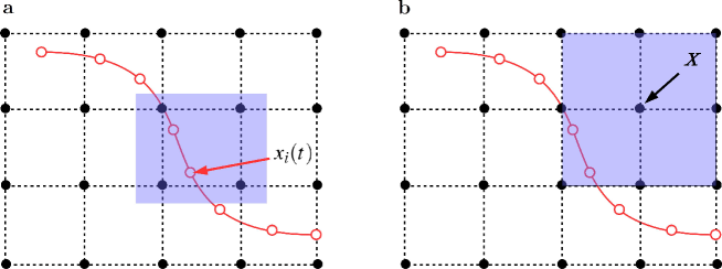
Figure 1: Schematic representation of the Immersed Boundary method. a. Interpolation step: the velocity of node $x_{i}(t)$ is interpolated from the lattice nodes inside the interpolation stencil. b. Spreading forces: the force density acting on the fluid node $X$ is obtained from the Lagrangian nodes inside the square region.

3.2 Constitutive model for the membrane of the immersed object

A regular mesh is used to approximate the surface of the immersed object. This could be a spherical or biconcave capsule if it represents a CTC or a RBC, respectively. Meridional and azimuthal angles are used to describe the surface of the immersed object. The advantage of using a parametric description of the mesh is that the local connectivity of each node of the network, i.e. its neighborhood structure, is simply induced by the equations of the geometric surface. This is particularly useful when the elastic forces are computed. Each Lagrangian node on the surface of the immersed object $x_{n,m}$ is identyfied by two parameters $0\leq n,m\leq N$ , such that the total number of points on the surface is $N^{2}$. The stretching force $F^{\rm s}$ acting on each Lagrangian node $x_{n,m}$ is defined by summing up the forces on the springs connected to its neighboring nodes $x_{n^{\prime},m^{\prime}}\in\{x_{n\pm 1,m},x_{n,m\pm 1}\}$ given by [44, 45]:

$$F^{\rm s}_{n,m}=-{\rm k}\sum_{n^{\prime},m^{\prime}}\dfrac{d_{n^{\prime},m^{\prime}}-d^{0}_{n,m}}{d^{0}_{n,m}}\dfrac{(x_{n^{\prime},m^{\prime}}-x_{n,m})}{d_{n,m}},$$ (7)

where $d_{n,m}=|x_{n^{\prime},m^{\prime}}-x_{n,m}|$ is the distance between node $x_{n,m}$ and its neighbor $x_{n^{\prime},m^{\prime}}$ and ${\rm k}$ is the shear elastic modulus. A simple bending term can be considered as:

$$F^{\rm b}_{n,m}=-{\rm k}^{\rm b}\sum_{j}\left(\dfrac{\theta_{j}-\theta^{0}_{j}}{\theta^{0}_{j}}\right)\hat{n}_{j},$$ (8)

where index $j$ runs over adjacent edges $\{(n,m),(n\pm 1,m\pm 1)\}$, $\theta_{j}$ are the angles between adjacent triangles sourranding point $x_{n,m}$ and $\hat{n}_{j}$ is the outward unit vector related to edge $j$. To enforce membrane incompressibility, a constraint on the total volume is needed:

$$F^{\rm v}_{n,m}=-{\rm k}^{\rm v}\left(1-\dfrac{V}{V^{0}}\right)A_{n,m}n_{n,m},$$ (9)

where ${\rm k}^{\rm v}$ is the volume constraint factor, $V^{0}$ and $V$ are the volumes of the immersed object in the reference and current configuration respectively, $n_{n,m}$ is the outward unit normal vector associated to the Lagrangian point $x_{n,m}$ and $A_{n,m}$ is the area of the triangular element defined by the three mesh points $\{x_{n,m},x_{n+1,m},x_{n,m+1}\}$. To evaluate the normal unit vector and the area $A_{n,m}$ consider $\xi_{1}=x_{n+1,m}-x_{n,m}$ and $\xi_{2}=x_{n,m+1}-x_{n,m}$, then the unit outward normal vector is $n_{n,m}=\xi_{1}\wedge\xi_{2}/|\xi_{1}\wedge\xi_{2}|$ and the area of the triangular element is $A_{n,m}=|\xi_{1}\wedge\xi_{2}|/2$. The volume is computed at each time iteration via the discrete Green theorem as $V=\sum_{T}n_{T}\cdot c_{T}A_{T}/3$, where the summation index runs over all triangles $T=\{x_{n,m},x_{n+1,m},x_{n,m+1}\}$, $n_{T}$ the unit normal vector to the surface associated to triangle $T$, $A_{T}$ is the area of the triangular element, and $c_{T}=(x_{n,m}+x_{n+1,m}+x_{n,m+1})/3$ is the baricenter of the triangle $T$. Another constraint is imposed on the conservation of the total surface of the cell:

$$F^{\rm a}_{n,m}=-{\rm k}^{\rm a}\left(1-\dfrac{A}{A_{0}}\right)\ \zeta_{n,m},$$ (10)

where ${\rm k}^{\rm area}$ is the area constraint factor and $\zeta_{n,m}$ is the unit vector pointing from the centroid of triangle $T=\{x_{n,m},x_{n+1,m},x_{n,m+1}\}$ to the vertex $x_{n,m}$ . This constraint is applied in the case of RBCs and CTCs to account for their cytoskeleton [46, 47].

3.3 Particle-particle interactions

The cell-cell interactions can be approximated with the Morse potential given by [13]:

$$U_{M}(r)=D_{e}(e^{2\beta(r_{0}-r)}-2e^{\beta(r_{0}-r)}),$$ (11)

where $r$ is the distance between two cells and $D_{e}$ is the energy well depth. Note that the calibration of the Morse potential can be done following the same procedure in [41] returning $D_{e}=0.04k_{B}T$, where $k_{B}T=4.14\times 10^{-21}N\cdot m$. Let $d_{n,m}=|x_{n,m}-x_{n^{\prime},m^{\prime}}|$ be the distance between two nodes on different structures. The interaction force between node $x_{n,m}$ on the surface of the current cell and node $x_{n^{\prime},m^{\prime}}$ on another cell is given by:

$$F^{\rm inte}_{n,m}=\begin{cases}-2\beta D_{e}U_{M}\dfrac{x_{n,m}-x_{n^{\prime},m^{\prime}}}{|x_{n,m}-x_{n^{\prime},m^{\prime}}|},&\text{if}\ d_{n,m}<d_{\rm cut}\\ 0,&\text{otherwise}.\end{cases}$$ (12)

The Morse interaction potential is implemented between two nodes of separate cells if they are within a cutoff distance $d_{\rm cut}$. This type of interaction consists of a high short-range repulsive force when $r<r_{0}$ and a low long-range attractive force for $r>r_{0}$. Parameters used are: $\beta=3.84\ \mu$m^-1, $r_{0}=0.5\ \mu$m, and $d_{\rm cut}=1.5\ \mu$m [13, 48].

3.4 Wall-particle interactions

Ligand and receptor molecules are distributed over the cell and blood vessel surfaces, respectively. Ligand molecules are modeled as linear springs which tend to establish bonds with receptors on the vascular wall. Let $x_{n,m}$ be a point on the particle surface, $x_{\rm wall}$ be the normal projection of $x_{n,m}$ on the wall of the channel, and $l_{n,m}=|x_{n,m}-x_{\rm wall}|$ be the distance between a point on the cell surface and the corresponding point on the wall, when the distance between the surface of the capsule and the wall is less than a critical distance $d_{\rm wall}$, the adhesive force acting on $x_{n,m}$ is defined as [34, 36]:

$$F^{\rm adh}_{n,m}=\begin{cases}-\sigma(l_{n,m}-\lambda)\dfrac{x_{n,m}-x_{\rm wall}}{l_{n,m}},\ &\text{if}\ d^{\rm w}_{n,m}<d_{\rm wall}\\ 0,\ &\text{otherwise}.\end{cases}$$ (13)

where $d^{\rm w}_{n,m}=d(x_{n,m},\rm wall)$ is the distance of $x_{n,m}$ from the wall, $\sigma$ is the adhesion constant, $\lambda$ is the equilibrium separation distance for the spring and $d_{\rm wall}=2\lambda$ is the critical distance. It is here important to recall that the mathematical model for cell-wall adhesion mediated by receptor-ligand interactions was originally presented by Hammer and colleagues and applied to study the rolling dynamics of leukocytes on endothelial surfaces [39]. Since then, this Adhesive-Dynamics model (AD) has been extended to study many biologically relevant problems, such as the hydrodynamic recruitment of rolling leukocytes [40], platelet-surface and platlet-platlet interactions [49, 50]. Note also that the current model does not account for the stochastic formation and rupture of ligand receptor bonds, which can be readily included following previous works by the authors and others [39, 40, 30].

4 Results and discussion

The proposed hierarchical computational model combines a Lattice-Boltzmann (LBM) algorithm, for solving the fluid flow, with an Immersed Boundary method (IBM), for determining particle-fluid and particle-wall interactions. As such, the computational model can efficiently deal with multiple scales and different biophysical problems, spanning from the ligand-receptor adhesive interactions (molecular scale) to the deformation of cell membranes (mesoscopic scale) and the transport of multiple red blood cells (RBCs) in a capillary flow (macroscopic scale). This is schematically presented in Fig.2. The computational model is first validated against known test cases: a deformable spherical capsule in a linear shear flow; the stretching of a red blood cell under uniaxial loading. Finally, the model is applied to document the vascular transport and adhesion dynamics of a single circulating tumor cells (CTCs), in whole blood flow, in microvessels of different calibers.

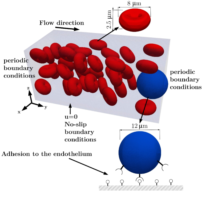
Figure 2: Schematic representation of a CTC in whole blood flow. A spherical, deformable circulating tumor cell (CTC) is transported downstream in a whole blood flow. The CTC interaction with the vessel wall is mediated by the formation of receptor-ligand bonds.

It is worth noting that in the present paper, only one CTC is considered. Given the low abundance of CTCs in blood, this condition is indeed physiologically sound. Other blood cells, such as leukocytes, platelets, monocytes and so on, are not explicitly modeled in this problem in that they are far less abundant than RBCs. Indeed, RBCs represent up to $95\%$ of all cellular components of blood and are responsible of the peculiar blood rheology. In small vessels, ranging from $10$ to $40\;\mu\rm m$, the volume fraction of RBCs varies from $15$ to about $35\%$ [18]. In the present work, the hematocrit has been fixed to the average value of $20\%$. Indeed, higher values for the hematocrit are associated with higher computational burden. The fluid solver used in this model relies on the Lattice-Boltzmann method which is very accurate and effective in terms of single cost per time iteration. However, a Lattice-Boltzmann solver is explicit in time and, as such, requires small time steps (in the order of $10^{-7}$ sec) to ensure stability. The effect of the mesh resolution on the accuracy of the solution is provided for the first test case.

4.1 A deformable spherical capsule in a linear shear flow: Test case 1

A spherical capsule of radius $r$ is placed in the center of a cubic box of size $L$ and subjected to a linear shear flow, realized by moving the top and bottom walls with velocities $u_{0}$ and $-u_{0}$, respectively (Fig.3a). The size of the fluid mesh is $L=16r$. $6400$ Lagrangian points are used to discretize the capsule membrane. The fluid is considered as quasi-stationary in the so-called Stokes regime with a Reynolds number $Re={10}^{-2}$ and a shear rate $\dot{\gamma}=\nu Re/r^{2}$, where $\nu=1/6$ is the lattice viscosity. Thus, the magnitude of the imposed velocity $u_{0}$ is given as $u_{0}=\dot{\gamma}L/2$. The capsule has a shear elastic modulus $k$. The capillary number ${\rm Ca}$ $({\rm Ca}=\dot{\gamma}\nu r/k)$, which represents the relative effect of the viscous drag over surface tension, provides a measure of the capsule deformability: ${\rm Ca}=0$ means a rigid capsule ($k\rightarrow+\infty$); ${\rm Ca}>0$ means a deformable capsule.
In a linear shear flow, the capsule rotates and deforms assuming eventually the shape of an ellipsoid (Fig.3b,c), with $r_{a}$ and $r_{b}$ being the two principal axes of the ellipsoid. Fig.3b gives the steady state, normalized velocity distribution $u/u_{0}$ within the box, for ${\rm Ca}=0.075$. Four recirculation areas are clearly developing around the elongated capsule. The deformation of the capsule is quantified via the Taylor parameter $D$ ($D=(r_{a}-r_{b})/(r_{a}+r_{b})$). Deformed configurations of the capsule at steady state are shown in Fig.3c for three representative values of the capillary number, namely ${\rm Ca}=0,0.075$ and $0.15$. Indeed, the larger is the capillary number, the larger is the capsule deformation $D$. This is also presented quantitatively in Fig.3d, where the Taylors number $D$ is plotted versus the non-dimensional time $\dot{\gamma}t$, for different values of the capillary number ${\rm Ca}(=0.0375,0.075,0.15$ and $0.3)$. $D$ increases with time until a steady state configuration is reached for $\dot{\gamma}t\geq 3$. For longer times, the capsule membrane rotates along its own shape with a inclination angle $\phi$, as predicted by the known tank-treading condition [51]. In Fig.3d, the present solution is compared with data from a neo-hookean membrane model, solved using the Boundary Integral method (BIM), by Lac and colleagues [51] for two values of the mesh resolution, namely low ($r=5,L=80$, dotted lines) and high ($r=10,L=160$, solid lines) resolution. The presented results are in good agreement with the BIM data, for different ${\rm Ca}$ values [51]. Notice that the agreement between the two solutions improves as the mesh resolution increases. This appears to be particularly relevant at large ${\rm Ca}$, which corresponds to more deformable capsule. The difference between the two numerical solutions is plotted as a function of ${\rm Ca}$ in Fig.3e, at steady state. This difference grows with the capillary number ${\rm Ca}$, as previously pointed out [45], but it stays well below $4\%$ for all considered cases. Table.1 summarizes the $D$ values for different ${\rm Ca}$ numbers obtained by BIM simulations and the current method, demonstrating that the difference ranges from $0.047\%$ for ${\rm Ca}=0.0375$ to $3.04\%$ for ${\rm Ca}=0.3$. In Table.2, are reported the values of the capsule angle $\phi/\pi$ for ${\rm Ca}=0.0375,0.075$ and $0.15$. The angle $\phi$ is computed as
$\phi=0.5\times\arctan\left(2r_{a}r_{b}/(r^{2}_{b}-r^{2}_{a})\right)$.

Figure 3: A deformable spherical capsule in a linear shear flow. a. Schematic representation of the problem and computational domain. b. Normalized velocity field at steady state (${\rm Ca}=0.075$). c. Steady state configurations of spherical capsules for ${\rm Ca}=0,0.075$, and $0.15$. d. Variation of the Taylor number $D$ with time, for ${\rm Ca}=0.0375,0075,0.15,$ and $0.3$ (dashed line: low resolution; solid line: high resolution; solid dots: BIM simulations by Lac et al. [51]). e, f. Percentage difference between BIM simulations and the present solution, at steady state, for different ${\rm Ca}$ and mesh resolutions (low resolution: $r=5$, $L=80$; high resolution $r=10$, $L=160$).

Table 1: Evolution of the Taylor parameter $\rm D$ as a function of the capillary number $\rm Ca$.

Ca	$\rm D$ Lac (2004)	$\rm D$ $(r=10,L=160)$	$\%$ Diff.	$\rm D$ $(r=5,L=80)$	$\%$ Diff.
0.0375	0.0798	0.0794	0.04	0.0790	0.080
0.075	0.1594	0.1487	1.07	0.1461	1.33
0.15	0.2718	0.2594	1.24	0.2491	2.49
0.3	0.4053	0.3904	1.49	0.3749	3.04

Table 2: Evolution of the inclination angle $\phi/\pi$ as a function of the capillary number $\rm Ca$.

Ca	$\phi/\pi$ Lac (2004)	$\phi/\pi$ $(r=5,L=80)$	$\%$ Diff.
0.0375	0.21739	0.21929	0.19
0.075	0.18391	0.19694	1.3030
0.15	0.15826	0.16401	0.5750

4.2 The stretching of a red blood cell under uniaxial loading: Test case 2

A single red blood cell (RBC) is stretched longitudinally by applying a force $\rm F$ at two opposite sites of the cell membrane (Fig.4a). After a transient phase, the elastic reaction force ${\rm F}^{\rm el}$ arising at the cell membrane balances out the external applied force $\rm F$ so that a steady deformation is achieved. This case serves to predict the stretching of a RBC in a pulling test realized using an optical tweezer [46, 47]. Briefly, two silica microbeads are attached at opposite sites of the cell membrane: one bead is anchored to the surface of a glass slide, while the other one is trapped by a laser beam. By moving the bead attached to the glass slide, a well defined strain is applied to the cell. At equilibrium, the diameter ${\rm D}_{a}$ in the pulling direction (axial) and the diameter ${\rm D}_{t}$ orthogonal to the pulling direction (transverse) are measured for each value of the applied force. This is documented by solid dots in Fig.4b. Experimentally the traction force $\rm F$ ranges from $0$ to $180$ pN.
The $3D$ shape of the RBC is given by the following parametric equations, for $0\leq\theta\leq 2\pi,0\leq\phi\leq\pi$:

$$\begin{cases}x=a\alpha\sin(\theta)\cos(\phi)\\ y=\dfrac{a}{2}(0.207+2.003\sin^{2}(\theta)-1.123\sin^{4}(\theta))\cos(\theta)\\ z=a\alpha\sin(\theta)\sin(\phi)\end{cases}$$ (14)

where $a=0.74{\rm r}_{\rm rbc}$, with ${\rm r}_{\rm rbc}=3.91\ \mu$m being the equivalent RBC radius and $\alpha=1.39$. Note that this parametric equation is equivalent to the well known Evans-Fung formula in cartesian coordinates [46, 52, 53]. The RBC shear modulus is taken as ${\rm k}_{\rm rbc}=8.3\ \mu$N$/$m [47]. The solid lines in Fig.4b report the values of ${\rm D}_{a}$ and ${\rm D}_{t}$ computed at equilibrium for different values of $\rm F$ via the present hierarchical model. As expected, the diameter ${\rm D}_{a}$ increases while ${\rm D}_{t}$ decreases with the applied force $\rm F$. The computed axial and transverse diameters ${\rm D}_{a}$ and ${\rm D}_{t}$ are in good agreement with the experimental data [47]. Fig.4c shows representative equilibrium configurations of the RBC under different applied forces. The proposed hierarchical model captures correctly the mechanical deformation of RBCs with an overall error lower than $10\%$. Values of the diameters $D_{a}$ and $D_{t}$ for different applied forces $F$ are reported in Table 3 and compared with experimental data by [47]. The RBC bending modulus ${\rm k}^{b}_{\rm rbc}$ and volume constraint ${\rm k}^{v}_{\rm rbc}$ can be estimated as previously documented in [18, 47], returning ${\rm k}^{b}_{\rm rbc}=2.4\times 10^{-19}$ J ($=0.0016$ in LB units) and ${\rm k}^{v}_{\rm rbc}=10$ (LB units).

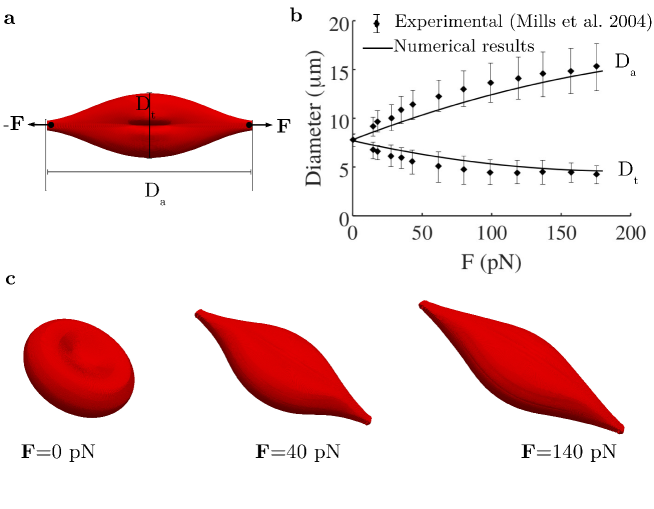
Figure 4: The stretching of a red blood cell under uniaxial loading. a. Schematic representation of the problem. Pulling force $\rm F$ is applied at two opposite sides of the RBC membrane. b. The variation of the axial and transverse diameters (${\rm D}_{a}$, ${\rm D}_{t}$) at steady state, for different pulling forces $\rm F$. (solid dots: experimental results from Mills et al. [47]; solid lines: present hierarchical model). c. Steady state configurations of a RBC subjected to an uniaxial pulling force $\rm F$ of $0,40$ and $140$ pN.

Table 3: Measured axial and transversal RBC diameters under a stretching test.

$\rm F$(pN)	${\rm D}_{a}$($\mu$m) Mills (2004)	${\rm D}_{a}$($\mu$m)	${\rm D}_{t}$($\mu$m) Mills (2004)	${\rm D}_{t}$($\mu$m)
20	9.65672 $\pm$ 1.08955	9.19057	6.61194 $\pm$ 0.73134	6.31599
40	11.41791 $\pm$ 1.50746	9.95102	5.58209 $\pm$ 1.22388	6.08232
60	12.23881 $\pm$ 1.61194	10.98340	5.09851 $\pm$ 1.56716	5.81418
100	13.64179 $\pm$ 2.01309	12.19840	4.44179 $\pm$ 1.26866	5.09710
120	14.08955 $\pm$ 2.14925	12.69840	4.40299 $\pm$ 1.20896	4.70220
140	14.58209 $\pm$ 2.31343	13.77490	4.50746 $\pm$ 1.22388	4.52800
160	14.83582 $\pm$ 2.32836	14.58190	4.46269 $\pm$ 1.01256	4.30200
180	15.34328 $\pm$ 2.41791	15.2200	4.25373 $\pm$ 0.94030	4.14313

4.3 Margination dynamics of circulating tumor cells with different deformability

Cancer spreading to distant tissues (metastasis) involves the shedding in the circulation of malignant cells from a primary lesion; their vascular transport, adhesion, extravasation and proliferation [54, 2, 3, 4]. During their journey, CTCs reach peripheral vascular beds, with blood vessels characterized by a diameter ranging between $10$ and $40\ \mu$m. In these small vessels, the presence of RBCs would favor the margination of CTCs towards the vascular endothelium, just like for leukocytes in an inflamed vessel. While the shear modulus of a RBC is in the range of ${\rm k}_{\rm rbc}=5-10\ \mu$N $/$m [46], CTC deformability can vary from fractions of $1$ kPa (soft) up to $100$ kPa, which is $20$ times higher than a RBC (rigid), under physiological conditions [55, 12]. In this section, the effect of cell deformability on CTC vascular dynamics is analyzed.
The proposed hierarchical computational model is applied to study the transport of an ensemble of RBCs and a single CTC within a capillary for an hematocrit of $20\%$, which is a physiological value in the microcirculation. It is well known that, due to their deformability, RBCs move away from the walls and migrate to the center of the capillary [13, 19, 56]. This results in the formation of a region depleted of cells next to the wall, which is called the cell-free layer (CFL). This non-Newtonian effect known as the Fåhræus-Lindqvist effect [19] is responsible for the modulation of the blood viscosity.

Following [41, 32], a capillary with a square cross section of $H=W$ and lenght $L$ is considered. The equivalent radius of the RBC is ${\rm r}_{rbc}=3.9\ \mu$m, so that $V_{\rm rbc}=94.1\mu$m³. Following the same equation described in the previous section, RBCs are modelled as biconcave membranes.
A number $N_{\rm rbc}$ of vectors, representing the RBC and CTC centers of mass, are uniformely generated in space and positioned in the volume $V_{\rm cap}$. Each RBC has initially a random orientation with respect to the $x$- and $z$- axes. For each RBC, the number of Lagrangian points is $4900$. Periodic boundary conditions are imposed in the flow direction at the inlet and outlet sections of the capillary, while no-slip velocity boundary conditions are prescribed on the remaining walls. Bounce-back boundary conditions are employed to treat the no-slip velocity conditions at the walls. The Reynolds number is fixed to be $Re=2.5\times{10}^{-2}$. The blood flow is driven by a constant body force density $\rho f$, which is equivalent to prescribe a pressure difference over the lenght of the capillary given by $\Delta P/L=16u_{0}\nu\rho/D^{2}$, where $u_{0}=\nu Re/H$ is the peak velocity in the flow direction, $D=4HW/2(H+W)=H$ is the hydraulic diameter of the channel. The non-dimensional time $\dot{\gamma}t$ is considered, where $\dot{\gamma}=4u_{0}/H$ is the shear rate. The capillary number is defined as ${\rm Ca}=\nu\dot{\gamma}{\rm r}_{\rm rbc}/{\rm k}_{\rm rbc}$ and fixed to $0.026$ for the RBCs. The Lattice resolution is $\Delta x=0.5714\ \mu$m and the Lattice-Boltzmann viscosity is given by $\nu=\frac{1}{6}\Delta x^{2}{\Delta t}^{-1}$. Note that, in dimensional units, the viscosity is equal to $\nu=1.2\times{10}^{-6}$ m²s^-1 and the plasma density is $\rho=1000$ Kg$/$m³. A capillary with a square cross section of $H=W=25\ \mu$m and lenght $L=60\ \mu$m is considered. The CTC is modelled as a spherical capsule having a radius ${\rm r}_{\rm ctc}=12\ \mu$m and discretized with $6400$ Lagrangian points. A Poiseuille flow with Reynolds number $Re=0.25\times{10}^{-2}$ is assumed. Periodic boundary conditions are prescribed at the front and back walls of the capillary, while no-slip velocity boundary conditions are imposed on the remaining walls. Table4 collects the values of all physical parameters used in this simulation. The initial position of the CTC center of mass is $(x_{0},y_{0},z_{0})=(W/2,L-2{\rm r}_{\rm ctc},H/2-{\rm r}_{\rm ctc})$.

Table 4: Table listing the parameters used in the simulations.

Parameters	Symbol	Value
Tube height, size	$H=W,D$	$25,15\ \mu$m
Tube segment lenght	$L$	$60\ \mu$m
RBC radius	${\rm r}_{\rm rbc}$	$4\ \mu$m
CTC radius	${\rm r}_{\rm ctc}$	$12\ \mu$m
RBC count	$N_{\rm rbc}$	Variable
Hematocrit	${\rm H_{t}}$	$N_{\rm rbc}V_{\rm rbc}/V_{\rm cap}$
Plasma kinetic viscosity	$\nu$	$1.2\times 10^{-6}$ m2/s
RBC stiffness modulus	${\rm k}_{\rm rbc}$	$10\mu$ N/m
RBC bending modulus	${\rm k}^{b}_{\rm ctc}$	$2.4\times 10^{-19}$ J
RBC volume constraint	${\rm k}^{v}_{\rm ctc}$	$10$
CTC stiffness modulus	${\rm k}_{\rm ctc}$	$5-200\mu$ N/m
Reynolds number	$Re$	$2.5\times 10^{-}2$
Center velocity (no cells)	$u_{0}$	$\nu Re/H$
Shear rate	$\dot{\gamma}$	$4u_{0}/H$
Pressure gradient	$f=\Delta p/L$	$16\nu\rho u_{0}/H^{2}$
Lattice resolution	$\Delta x$	$0.5714\ \mu$m
Time step	$\Delta t$	$\Delta x^{2}/6\nu$
Capillary number	${\rm Ca}$	$\nu\dot{\gamma}{\rm r}_{\rm rbc}/{\rm k}_{\rm rbc}$
Adhesive number	$Ad$	$\sigma/\nu\dot{\gamma}{\rm r}_{\rm rbc}$
Receptor-ligand resting lenght	$\lambda$	$50$ nm

Three different CTC deformability values are considered: a CTC softer than RBCs (${\rm k}_{\rm ctc}=0.5{\rm k}_{\rm rbc}$: SOFT); a CTC stiffer than RBCs (${\rm k}_{\rm ctc}=10{\rm k}_{\rm rbc}$: RIGID); a CTC as deformable as a RBC (${\rm k}_{\rm ctc}={\rm k}_{\rm rbc}$: EQUAL). Fig.5a,c show the RBC distribution and the CTC location within a longitudinal section of the capillary, at time $\dot{\gamma}t=100$, for the ‘soft’, ‘rigid’ and ‘equal’ cases. On the right, fluid velocity profiles are shown. Specifically, the different velocity profiles are referred to the classical Poiseuille case in the absence of RBCs (black line); the time-averaged velocity profile for ${\rm H_{t}}=20\%$ with RBCs and no CTC (red line); and the time-averaged velocity profile for ${\rm H_{t}}=20\%$ with RBCs and the CTC (blue line). The presence of the CTC does not change significantly the time-averaged velocity profile, whereas the addition of RBCs flattens the classical Poiseuille parabolic profile, as well documented in the literature. In the ‘rigid’ case (${\rm k}_{\rm ctc}=10{\rm k}_{\rm rbc}$), malignant cells are rapidly pushed out from the center of the capillary and confined to move within the CFL (Fig.5b). This indeed increases the likelihood of building adhesive interactions with the wall. For the other two cases (${\rm k}_{\rm ctc}=0.5{\rm k}_{\rm rbc}$ and ${\rm k}_{\rm ctc}={\rm k}_{\rm rbc}$), malignant cells are not observed to marginate within the considered simulation time. This is due to the fact that RBCs and CTCs would move similarly in the channel, deforming under flow and moving away from the walls (Fig.5b,c).
In Fig.5d, the CTC trajectories are presented for the three considered cases. In the ‘soft’ and ‘equal’ cases (red and blue lines), malignant cells migrate towards the centerline $z=H/2$ and stay within the capillary core without interacting with the vessel walls throughout the simulation time. Conversely, in the ‘rigid’ case, malignant cells deviate from the streamlines and, eventually, reach the capillary wall (margination). For these simulations, the cell-wall adhesion potential is turned off and a moderate repulsive force is included only to prevent body compenetration.

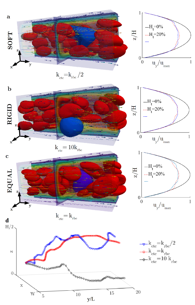
Figure 5: Margination dynamics of a CTC with different deformability in whole blood flow. a-c. Representative images of RBC and CTC distribution within a capillary whole blood flow (${\rm H_{t}}=20\%,D=25\ \mu$m) for the ‘rigid’ (a), ‘soft’ (b) and ‘equal’ (c) cases. The right columns show the velocity profile compared to the pure plasma parabolic profile. d. Trajectories of the center of mass of the CTC for ${\rm k}_{ctc}=\{{\rm k}_{rbc}/2,{\rm k}_{rbc},10{\rm k}_{rbc}\}$ (black line: ${\rm k}_{ctc}=10{\rm k}_{rbc}$; blue line: ${\rm k}_{ctc}={\rm k}_{rbc}/2$ ; red line: ${\rm k}_{ctc}={\rm k}_{rbc}$).

4.4 Adhesion dynamics of circulating tumor cells in a large microcapillary: the $25\mu\rm m$ case

After marginating towards the vessel walls, CTCs could firmly adhere to the endothelial cells, if proper conditions are met. The margination and vascular adhesion are fundamental steps in the cascade of events regulating the extravasation of both leukocytes, in inflammation, and CTCs, in metastasis. Adhesive interactions are governed by receptor molecules, expressed on the vascular endothelial cells and ligand molecules, distributed over the CTC membrane (Fig.2). These molecular interactions operate only, and only if, CTCs are sufficiently close to the wall, namely closer than a critical distance set to $d_{\rm wall}=100\ \rm nm$. The molecular bonds are computationally treated as linear springs, whose strength is dictated by the adhesive number $\rm Ad=\sigma/\nu\dot{\gamma}{\rm r}_{\rm ctc}$. Simulations are performed by fixing a value of the adhesive strenght $\sigma$ and varying the CTC stiffness ${\rm k}_{\rm ctc}$. In this section, the proposed hierarchical computational model is applied to predict the vascular adhesion dynamics of CTCs as a function of their deformability.

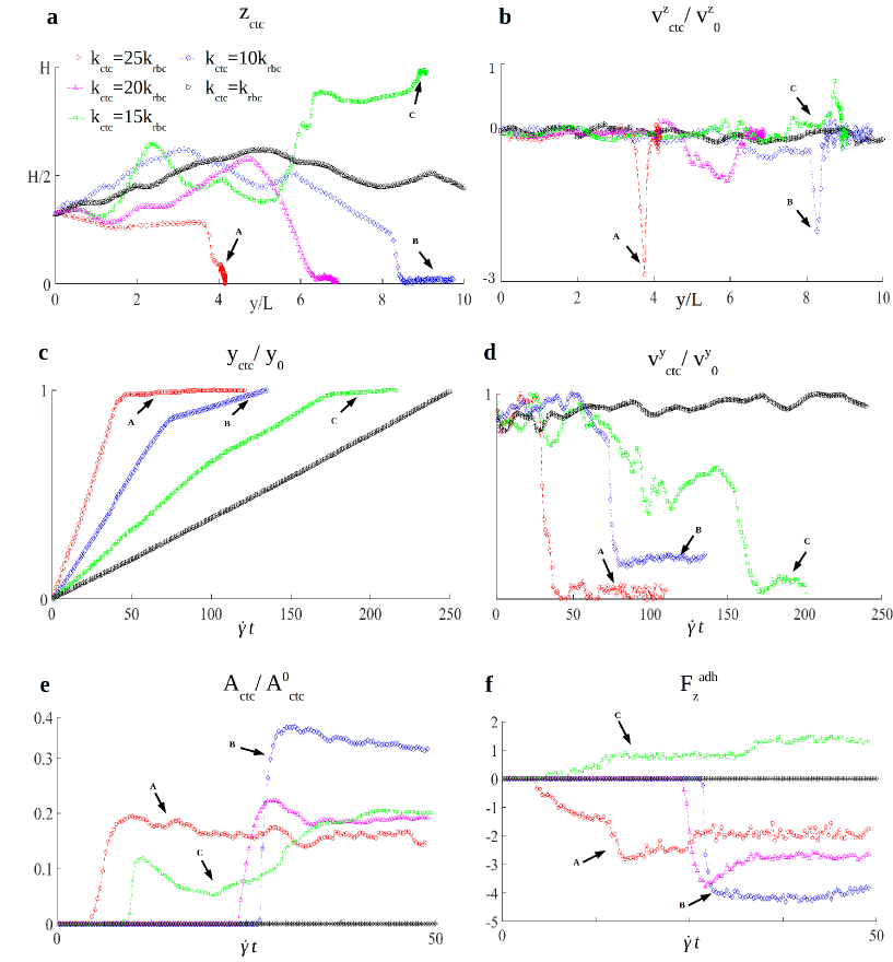
Figure 6: Adhesion dynamics of a CTC in a large microcapillary ($25\mu\rm m$ case). a.Variation over the capillary length $y/L$ of the vertical position $z_{\rm ctc}/z_{0}$ of the CTC, for different values of ${\rm k}_{\rm ctc}$. b. Variation over the capillary length $y/L$ of the vertical CTC velocity $v^{z}_{\rm ctc}/v^{0}_{z}$, for different values of ${\rm k}_{\rm ctc}$. c. Variation of the normalized coordinate along the flow $y_{\rm ctc}/y_{0}$ of the CTC over time $\dot{\gamma}t$, for different values of ${\rm k}_{\rm ctc}$. d. Variation of the normalized velocity along the flow $v^{y}_{\rm ctc}/v^{y}_{0}$ of the CTC over time $\dot{\gamma}t$, for different values of ${\rm k}_{\rm ctc}$. e. Variation of the contact area $A_{\rm ctc}/A^{0}_{\rm ctc}$ of the CTC over time $\dot{\gamma}t$. f. Variation of the vertical component of the adhesion force $F^{\rm adh}_{z}$ of the CTC over time $\dot{\gamma}t$. (black line: ${\rm k}_{\rm ctc}={\rm k}_{\rm rbc}$; blue line: ${\rm k}_{\rm ctc}=10{\rm k}_{\rm rbc}$; green line: ${\rm k}_{\rm ctc}=15{\rm k}_{\rm rbc}$; violet line: ${\rm k}_{\rm ctc}=20{\rm k}_{\rm rbc}$; red line: ${\rm k}_{\rm ctc}=25{\rm k}_{\rm rbc}$).

Based on the results of the previous paragraph, the CTC stiffness is here assumed to be high enough to allow rapid margination, namely ${\rm k}_{\rm ctc}=10,15,20$ and $25{\rm k}_{\rm rbc}$. For soft CTCs, margination would not occur in capillaries with a tube size of $D=25\ \mu$m, within the time of the simulations. Indeed, this implies that soft CTCs could interact with the vascular walls only in capillaries slightly larger, or even smaller, than the CTC tube size, as shown in the sequel. The relative position of CTCs, the size of the adhesion area and the adhesion forces are monitored over time. The CTC dynamics is presented in Fig.6a,b in terms of the vertical coordinate $z_{\rm ctc}(y)$ and corresponding velocity component $v^{z}_{\rm ctc}(y)$ as a function of the position along the $y$-axis, and of the horizontal coordinate $y_{\rm ctc}(t)$ and corresponding velocity component $v^{y}_{\rm ctc}(t)$ as a function of time (Fig.6c,d). The $z$-direction is normal to the flow, whereas the $y$-direction is aligned with the flow.
In Fig.6a the black line corresponds to ‘soft’ CTCs (${\rm k}_{\rm ctc}={\rm k}_{\rm rbc}$) for which margination does not occur within the considered simulation time. In this case, the vertical position $z_{\rm ctc}$ of the CTC oscillates sligthly around the centerline of the capillary ($z=H/2$) while the cell is transported downstream. This is also confirmed by the variation over time of $y_{\rm ctc}$, as shown in Fig.6c. The black line grows steadily over time implying that the CTC is steadily moving along the flow direction. As such, the velocity components $v^{z}_{\rm ctc}$ along $z$, in Fig.6b and $v^{y}_{\rm ctc}$ along $y$ in Fig.6d are, respectively, nearly zero and quasi-constant but larger than zero. Correspondingly, the size of the adhesion area $A_{\rm ctc}$ and adhesion force $F^{\rm adh}_{z}$ are both null (Fig.6e and f).
A totally different behavior is documented for ‘rigid’ CTCs (${\rm k}_{\rm ctc}=25{\rm k}_{\rm rbc}$), as per the red lines in Figs.6. The cell is pushed downstream by the flow but also laterally towards the vessel walls until a stable adhesion is established (point A). This is documented in Figs.6a and c by the reduction of $z_{\rm ctc}$ till zero (interaction with the lower vessel wall) and final constant value of $y_{\rm ctc}$. Also the velocity goes to zero, after a significant spike in $v^{z}_{\rm ctc}$ due to the margination process (point A in Fig.6b). The area of adhesion $A_{\rm ctc}$ grows upon interaction with the vessel wall and stays quasi-constant over time (Fig.6e). Similar observations apply for the adhesion force $F^{\rm adh}$ (Fig.6f). This is consistent with the stable adhesion of a relatively rigid cell that does not squeeze down onto the wall. The case ${\rm k}_{\rm ctc}=10{\rm k}_{\rm rbc}$ is depicted in Figs.6 by blue lines. The behavior is quite similar to that of ${\rm k}_{\rm ctc}=25{\rm k}_{\rm rbc}$, whereby the cell moves downstream and laterally towards the vessel wall and starts interacting with its surface. However, the margination process occurs over a longer time (see Fig.6a and c), with a smoother variation in the velocities (see Figs.6b and d). Interestingly, and differently from the more rigid case, the CTC preserves a non-zero $v^{y}_{\rm ctc}$ velocity, which implies that firm adhesion is not established but the cell is rather rolling steadly over the vessel wall (point B). Similarly, the size of the adhesion area and the value of the adhesion force do not change significantly over time after an initial increase (see Figs.6e and f). The stable rolling is supported by the continuous rupture and formation of ligand-receptor bonds, respectively, of the tail and leading edge of the adhesive area. Finally, the case ${\rm k}_{\rm ctc}=15{\rm k}_{\rm rbc}$ is depicted by the green line, in Figs.6. Under this condition, the CTC exhibits an even slower approach to the vessel wall. Also adhesion does not appear to be firm and complete suggesting a ‘crawling’ behavior over the vessel wall (point C). The velocity $v^{y}_{\rm ctc}$ is close to zero but not null (Fig.6d), the adhesion area grows steadily with time just like for the adhesion force documenting a progressive CTC flattening over the wall (see Figs.6e and f). Indeed, the higher CTC deformability favors its continuous deformation and conformation to the vessel walls under hemodynamic forces.
Figs.7 shows the RBC distribution and velocity field around the CTC under firm adhesion (Fig.7a) and steady rolling (Fig.7b) at different time points. Fig.7a shows images of the CTC undergoing firm adhesion on the vessel wall, after margination at different time points (${\rm k}_{\rm ctc}=25{\rm k}_{\rm rbc}$). When the CTC reaches the substrate, the adhesion force dominates over the lift hydrodynamic force. In this case the cell firmly adheres to the wall and experiences small variations in configurations due to the complex whole blood flow dynamics. The streamlines of the velocity $u/u_{0}$ show the initiation of a local recirculation area around the adhering CTC. The adhered CTC becomes an obstacle for the red blood cells, which are continuously hitting over the trailing edge of the CTC, and might detach the cell if adhesion is insufficiently strong. In Fig.7b, a CTC undergoing stable rolling dynamics on the wall is shown (${\rm k}_{\rm ctc}=10{\rm k}_{\rm rbc}$). The CTC moves along the vessel wall with a constant size of the adhesion area at the interface between the particle and the substrate. The rolling behaviour is confirmed by following the red spot on the cell membrane over time. It can be appreciated the increase of the contact area over time which is associated with the progressive flattening of the CTC over the vessel wall. Although a simplified adhesive model is used based on elastic springs, it is capable to predict different adhesive regimes. In particular, it is observed that, if sufficiently soft, CTCs can detach from the wall of a capillary.

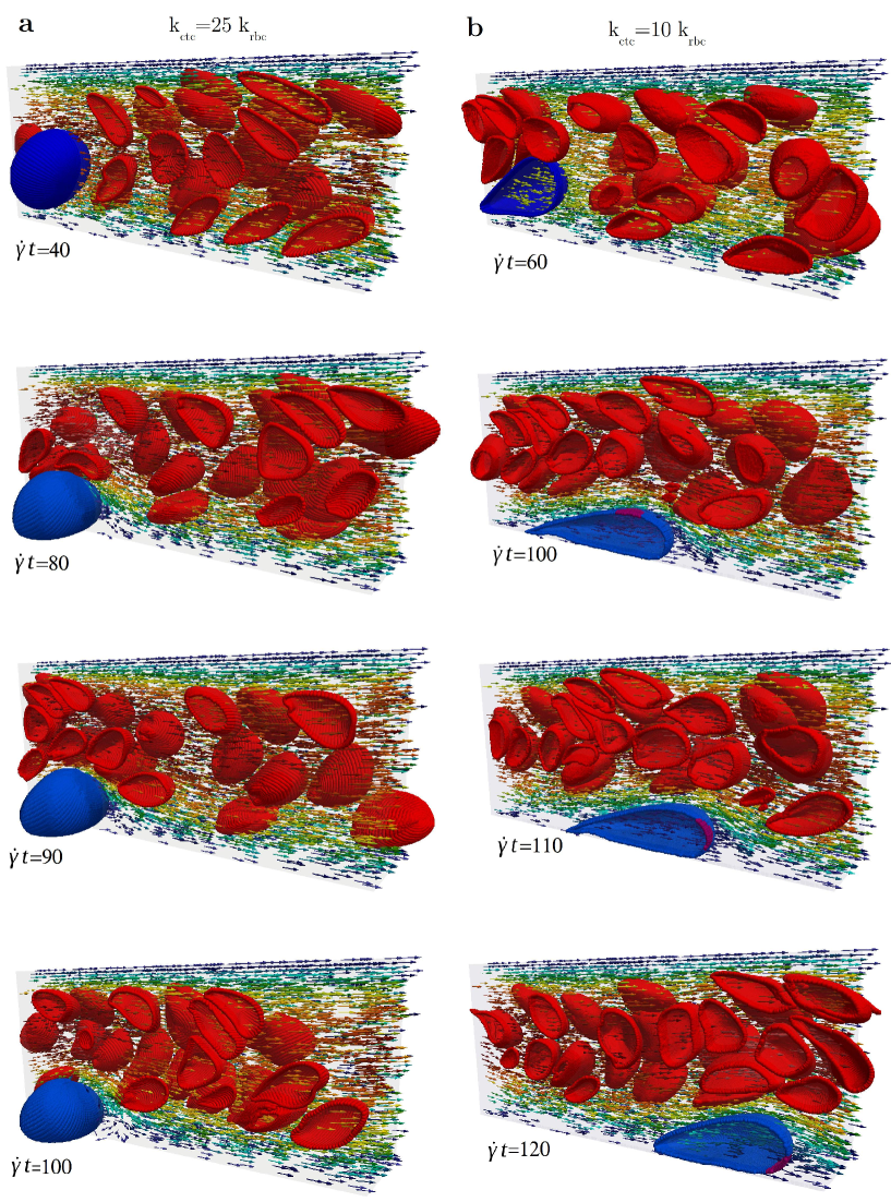
Figure 7: Adhesion dynamics of a CTC in a large microcapillary ($25\mu\rm m$ case). a. Section of the capillary showing a CTC firmly adhering on the endothelium (${\rm k}_{\rm ctc}=25{\rm k}_{\rm rbc}$). b. Section of the capillary showing a CTC rolling on the bottom of the endothelium (${\rm k}_{\rm ctc}=10{\rm k}_{\rm rbc}$). A small portion of the boundary of the cell is labelled in magenta.

4.5 Adhesion dynamics of circulating tumor cells in a small microcapillary: the $15\mu\rm m$ case

The analysis of the margination and adhesion process is here conducted in a capillary having a tube size comparable with the size of the CTC. The relative position of CTCs, the size of the adhesion area and the adhesion forces are monitored over time. The CTC dynamics is presented in Fig.8a,b in terms of the vertical coordinate $z_{\rm ctc}(y)$ and corresponding velocity component $v^{z}_{\rm ctc}(y)$ as a function of the position along the $y$-axis, and of the horizontal coordinate $y_{\rm ctc}(t)$ and corresponding velocity component $v^{y}_{\rm ctc}(t)$ as a function of time. The red and blue lines in Fig.8a,b correspond to ‘rigid’ CTCs, with ${\rm k}_{\rm ctc}=25{\rm k}_{\rm rbc}$ and ${\rm k}_{\rm ctc}=20{\rm k}_{\rm rbc}$. For these values, the vertical position $z_{\rm ctc}$ remains close to the centerline of the capillary ($z=H/2$). Correspondingly, $y_{\rm ctc}$ (red and blue lines in Fig.8c) is linearly increasing in time. As such, the velocity components $v^{z}_{\rm ctc}$ along $z$, in Fig.8b and $v^{y}_{\rm ctc}$ along y in Fig.8d are, respectively, nearly zero and quasi-constant but larger than zero. Also, for ‘rigid’ CTCs (${\rm k}_{\rm ctc}=25{\rm k}_{\rm rbc},{\rm k}_{\rm ctc}=20{\rm k}_{\rm rbc}$), the size of the adhesion area $A_{\rm ctc}$ and adhesion force $F^{\rm adh}$ are both null (Fig.8e and f). In the ‘rigid’ case, CTCs are transported along the flow direction by the fast moving RBCs and do not appear to be interacting with the vessel walls. Very different is the behavior observed for a ‘soft’ CTCs. This is shown in Fig.8a (green line: ${\rm k}_{\rm ctc}=10{\rm k}_{\rm rbc}$ ; violet line: ${\rm k}_{\rm ctc}=5{\rm k}_{\rm rbc}$ ; and black line: ${\rm k}_{\rm ctc}={\rm k}_{\rm rbc}$). $z_{\rm ctc}$ increases till the top capillary wall is reached. Spikes in the velocity component $v^{z}_{\rm ctc}$ (green, violet and black line in Fig.8b) demonstrate the interaction with the top wall and the subsequent establishment of adhesive interactions. In Fig.8c the components in the flow direction $y_{\rm ctc}$ for ‘soft’ CTCs, slightly deviate from the straight line and the velocity component $v^{y}_{\rm ctc}$ decreases, as in Fig.8d (green, violet and black line). This implies that the cell is no longer in the fluid phase and has established an adhesive interaction with the vessel walls. In Fig.8e,f, the variations of the contact area and adhesion force are shown for ‘soft’ CTCs (green, violet and black line). In all the cases, the contact area and the adhesion force increases with time. This is due to the interaction with RBCs and hydrodynamic lift force, which affects the formation of the contact area.

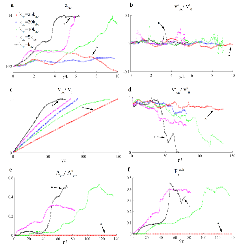
Figure 8: Adhesion dynamics of a CTC in a small microcapillary ($15\mu\rm m$ case). a.Variation over the capillary length $y/L$ of the vertical position $z_{\rm ctc}/z_{0}$ of the CTC, for different values of ${\rm k}_{\rm ctc}$. b. Variation over the capillary length $y/L$ of the vertical CTC velocity $v^{z}_{\rm ctc}/v^{z}_{0}$, for different values of ${\rm k}_{\rm ctc}$. c. Variation of the normalized coordinate along the flow $y_{\rm ctc}/y_{0}$ of the CTC over time $\dot{\gamma}t$, for different values of ${\rm k}_{\rm ctc}$. d. Variation of the normalized velocity along the flow $v^{y}_{\rm ctc}/v^{y}_{0}$ of the CTC over time $\dot{\gamma}t$, for different values of ${\rm k}_{\rm ctc}$. e. Variation of the contact area $A_{\rm ctc}/A^{0}_{\rm ctc}$ of the CTC over time $\dot{\gamma}t$. f. Variation of the vertical component of the adhesion force $F^{\rm adh}_{z}$ of the CTC over time $\dot{\gamma}t$. ( black line: ${\rm k}_{\rm ctc}={\rm k}_{\rm rbc}$; red line: ${\rm k}_{\rm ctc}=25{\rm k}_{\rm rbc}$; blue line: ${\rm k}_{\rm ctc}=20{\rm k}_{\rm rbc}$; green line: ${\rm k}_{\rm ctc}=10{\rm k}_{\rm rbc}$; violet line: ${\rm k}_{\rm ctc}=5{\rm k}_{\rm rbc}$).

Fig9.a shows images of a CTC undergoing ‘train’ dynamics in a small capillary ($D=15\ \mu$m) , at different time points for ${\rm k}_{\rm ctc}=25{\rm k}_{\rm rbc}$. The ‘rigid’ CTC is transported downstream without marginating. This results in a stable dynamics in which the CTC becomes a moving obstacle inside the capillary. The RBCs pile up behind the cell and form a dense aggregate [57]. Fig9.b shows representative images of the dynamics of a ‘soft’ CTC (${\rm k}_{\rm ctc}={\rm k}_{\rm rbc}$) in a small capillary. Due to its deformability the cell interacts with the vessel walls establishing adhesion. This results in a partial occlusion of the capillary. RBCs tend to pile up behind the cell, continuously pushing the cell against the wall, until they are free to pass again.
It can be concluded that in small capillaries of size comparable with that of the CTC, the stiffness of the cell is responsible for a transition from a ‘train’ dynamics, in which the CTC moves along the capillary without interacting with the walls (‘rigid’ case), to margination and subsequent adhesion dynamics (‘soft’ case).

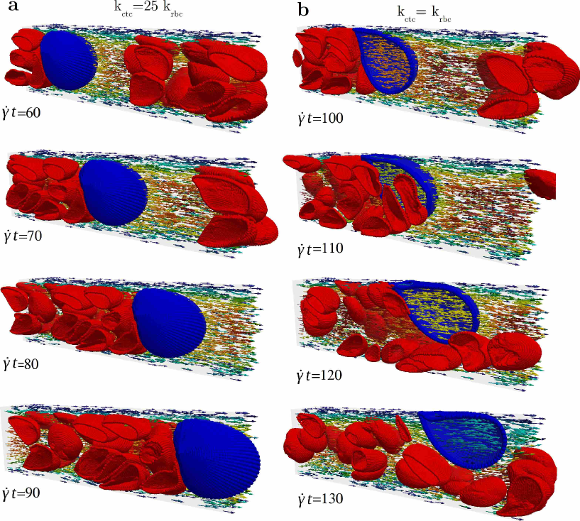
Figure 9: Adhesion dynamics of a CTC in a small microcapillary ($15\mu\rm m$ case). a. Section of the channel showing the so called ‘train’ dynamics of a CTC (${\rm k}_{\rm ctc}=25{\rm k}_{\rm rbc}$). b. Section of the capillary showing a CTC progressively adhering on the top of the capillary (${\rm k}_{\rm ctc}={\rm k}_{\rm rbc}$).

5 Conclusions

Using a combined Lattice Boltzmann-Immersed Boundary method, the transport of deformable CTCs in a whole blood capillary flow has been analyzed in terms of cell displacements and velocities, and cell interactions with the vessel walls. The evolution over time of the area of adhesion and adhesion forces exchanged at the cell-wall interface has been documented for CTC stiffer, softer and equally deformable as compared to RBCs. It has been demonstrated that the interaction between deformable CTCs and RBCs is crucial in shaping the metastatic process.
Rigid CTCs have been observed to marginate rapidly within $25\ \mu$m microcapillaries and efficiently interact with the vessel walls as they are pushed laterally by the RBCs. On the contrary, in smaller $15\ \mu$m microcapillaries, rigid CTCs cannot establish firm interactions with the vessel walls. This should be ascribed to the significant flow obstruction induced by a rigid CTC adhering in such a small vessel. In other words, the fast moving RBCs in $15\ \mu$m microcapillaries form a compact train that constantly pushes and dislodge downstream any obstacle, such as a rigid CTC. Different adhesive regimes have been predicted for the rigid CTCs depending on their relative stiffness to RBCs. Very rigid CTC would firmly adhere, if proper local hemodynamic and biophysical conditions ar met. Intermediate rigid CTCs would roll over the vascular walls, whereas CTCs that are slightly stiffer than RBCs could crawl over the surface as a combination of rolling and progressive squeezing against the wall. Soft CTCs have been observed to deform and navigate together with the RBCs in the core of the blood vessel in $25\ \mu$m microcapillaries. Very differently, in smaller $15\ \mu$m microcapillaries, soft CTCs can deform and squeeze progressively within the train of fast moving RBCs and the vessel walls. This indeed increases the surface area of the CTC exposed to the vessel wall and inevitably favors firm adhesion. As a consequence, soft CTCs are expected to have a higher longevity in blood and, possibly, the ability to evade more efficiently than rigid CTC the recognition by cells of the immune system. These findings highlight the role of CTC deformability in defining the metastatic potential of cancer cells.

6 Acknowledgements

This project was partially supported by the European Research Council, under the European Union’s Seventh Framework Programme (FP7/2007-2013)/ERC grant agreement no. 616695, by the Italian Association for Cancer Research (AIRC) under the individual investigator grant no. 17664, and by the European Union’s Horizon 2020 research and innovation programme under the Marie Skłodowska-Curie grant agreement no. 754490.

7 Conflicts of interest

Dr. Lenarda, Dr. Coclite and Dr. Decuzzi declare that they have no conflicts of interest.

8 Ethical standards

No animal studies or experiments with human samples were carried out by the authors for this article.

References

- [1] D. X. Nguyen, P.D. Bos, and J. Massagué. Metastasis: from dissemination to organ-specific colonization. Nat. Rev. Cancer, 9(4):274–284, 2009.
- [2] D. Wirtz, K. Konstantopoulos, and P. C. Searson. The physics of cancer: The role of physical interactions and mechanical forces in metastasis. Nat. Rev. Cancer, 11(7):512–522, 2011.
- [3] J. A. Joyce and J. W. Pollard. Microenvironmental regulation of metastasis. Nat. Rev. Cancer, 9(4):239–252, 2009.
- [4] H. Mollica, C. Coclite, M.E. Miali, R.C. Pereira, L. Paleari, C. Manneschi, A. DeCensi, and P. Decuzzi. Deciphering the relative contribution of vascular inflammation and blood rheology in metastatic spreading. Biomicrofluidics, 12(4):042205, 2018.
- [5] M.R. King, K.G. Phillips, A. Mitrugno, T.R. Lee, A.M. de Guillebon, S. Chandrasekaran andM.J. McGuire, R.T. Carr, S.M. Baker-Groberg, R.A. Riggand, A. Kolatkar, M. Luttgen, K. Bethel, P. Kuhn, P. Decuzzi, and O.J. McCarty. A physical sciences network characterization of circulating tumor cell aggregate transport. Am J Physiol Cell Physiol, 308(10):C792–C802, 2015.
- [6] S. J. Tan, L. Yobas, G. Y. Lee, C. N. Ong, and C. T. Lim. Microdevice for the isolation and enumeration of cancer cells from blood. Biomed Microdevices, pages 883–892, 2009.
- [7] E. Sollier, D. E. Go, J. Che, D. R. Gossett, S. O’Byrne, W. M. Weaver, N. Kummer, M. Rettig, J. Goldman, N. Nickols, S. McCloskey, R. P. Kulkarni, and D. Di Carlo. Size-selective collection of circulating tumor cells using vortex technology. Lab Chip, 14:63–77, 2014.
- [8] R. Riahi, P. Gogoi, S. Sepehri, Y. Zhou, K. Handique, J. Godsey, and Y. Wang. A novel microchannel-based device to capture and analyze circulating tumor cells (ctcs) of breast cancer. Int J Oncol, 44:1870–8, 2014.
- [9] M. Lekka, P. Laidler, D. Gil, J. Lekki, Z. Stachura, and A. Z. Hrynkiewicz. Elasticity of normal and cancerous human bladder cells studied by scanning force microscopy. Eur Biophys J, 28:312–6, 1999.
- [10] T. W. Remmerbach, F. Wottawah, J. Dietrich, B. Lincoln, C. Wittekind, and J. Guck. Oral cancer diagnosis by mechanical phenotyping. Cancer ResEur Biophys J, 69:1728–32, 2009.
- [11] S. E. Cross, Y. S. Jin, J. Rao, and J. K. Gimzewski. Nanomechanical analysis of cells from cancer patients. Nat Nanotechnol, 2:780–3, 2007.
- [12] J. Shaw Bagnall, S. Byun, S. Begum, D. T. Miyamoto, V. C. Hecht, S. Maheswaran, S. L. Stott, M. Toner, R. O. Hynes, and S. R. Manalis. Deformability of tumor cells versus blood cells. Sci Rep, 5:18542, 2015.
- [13] J. Zhang, P.C. Johnson, and A.S. Popel. Effects of erythrocyte deformability and aggregation on the cell free layer and apparent viscosity of microscopic blood flows. Microvasc. Res., 77(3):265–272, 2009.
- [14] R. Skalak. Strain energy function of red blood cell membranes. Biophys J, 13(3):245–264, 2009.
- [15] F. Varnik T. Krüger and D. Raabe. Efficient and accurate simulations of deformable particles immersed in a fluid using a combined immersed boundary lattice boltzmann finite element method. Computers and Mathematics with Applications, 61(12):3485–3505, 2011.
- [16] U.D. Schiller, T. Krüger, and O. Henrich. Mesoscopic modelling and simulation of soft matter. Soft Matter, 14(1):9–26, 2017.
- [17] C. Pozrikidis. Numerical simulation of the flow-induced deformation of red blood cells. Annals of Biomedical Engineering, 31(10):1194–1205, 2003.
- [18] D.A. Fedosov, B. Caswell, and G.E. Karniadakis. A multiscale red blood cell model with accurate mechanics. Biophysical Journal, 98(10):2215–2225, 2010.
- [19] D.A. Fedosov, B. Caswell, A.S. Popel, and G.E. Karniadakis. Blood flow and cell-free layer in microvessels. Microcirculation, 17(8):615–628, 2010.
- [20] D.A. Fedosov and G. Gompper. White blood cell margination in microcirculation. Soft Matter, 10(8):2961–70, 2014.
- [21] D.A. Fedosov, M. Peltmäki, and G. Gompper. Deformation and dynamics of red blood cells in flow through cylindrical microchannels. Soft Matter, 10(24):4258–67, 2014.
- [22] C.S. Peskin. The immersed boundary method. Acta Numerica, 11(3-4):479–511, 2002.
- [23] A. Saadat, G. Christopher J., G. Iaccarino, and E.S.G. Shaqfeh. Immersed-finite-element method for deformable particle suspensions in viscous and viscoelastic media. Phys. Rev. E, 98:063316, 2018.
- [24] Tae-Rin Lee, Myunghwan Choi, Adrian M Kopacz, Seok-Hyun Yun, Wing Liu, and Paolo Decuzzi. On the near-wall accumulation of injectable particles in the microcirculation: Smaller is not better. Scientific reports, 3:2079, 06 2013.
- [25] Ying Li, Wylie Stroberg, Tae-Rin Lee, Hansung Kim, Han Man, Dean Ho, Paolo Decuzzi, and Wing Liu. Multiscale modeling and uncertainty quantification in nanoparticle-mediated drug/gene delivery. Computational Mechanics, 53:511–537, 03 2014.
- [26] G. Falcucci, S. Ubertini, D. Chiappini, and S. Succi. Modern lattice boltzmann methods for multiphase microflows. IMA Journal of Applied Mathematics, 76(5):712–725, 2011.
- [27] S. Succi. Lattice boltzmann across scales: from turbulence to dna translocation. European Physical Journal B, 64(3-4):471–479, 2008.
- [28] S. Succi, G. Amati, M. Bernaschi, G. Falcucci, M. Lauricella, and A. Montessori. Towards exascale lattice boltzmann computing. Computers and Fluids, 181:107–115, 2019.
- [29] C. Sun, C. Migliorini, and L.L. Munn. Red blood cells initiate leukocyte rolling in postcapillary expansions: a lattice boltzmann analysis. Biophys J, 85(1):208–22, 2003.
- [30] A. Coclite, H. Mollica, S. Ranaldo, G. Pascazio, M. D. de Tullio, and P. Decuzzi. Predicting different adhesive regimens of circulating particles at blood capillary walls. Microfluidics and Nanofluidics, 21(11):168, 2017.
- [31] X. Yin and J. Zhang. Cell-free layer and wall shear stress variation in microvessels. Biorheology, 49:261–70, 07 2012.
- [32] H. Ye, Z. Shen, and Y. Li. Shear rate dependent margination of sphere-like, oblate-like and prolate-like micro-particles within blood flow. Soft Matter, 14(36):7401–7419, 2018.
- [33] S. Gekle. Strongly accelerated margination of active particles in blood flow. Biophysical Journal, 110(2):514 – 520, 2016.
- [34] K.A. Rejniak. Circulating tumor cells: When a solid tumor meets a fluid microenvironment. Front Oncol, 2(111), 2012.
- [35] W.W. Yan, Y. Liu, and B.M. Fu. Effects of curvature and cell-cell interaction on cell adhesion in microvessels. Biomech. Model. Mechanobiol, 9(5):629–40, 2010.
- [36] L.L Xiao, Y. Liu, S. Chen, and B.M. Fu. Effects of flowing rbcs on adhesion of a circulating tumor cell in microvessels. Biomech. Model. Mechanobiol, 16(2):597–610, 2017.
- [37] S. Succi. The lattice Boltzmann equation: for fluid dynamics and beyond. Oxford University Press, 2001.
- [38] Vesselin Krassimirov Krastev and Giacomo Falcucci. Simulating engineering flows through complex porous media via the lattice boltzmann method. Energies, 11(4), 2018.
- [39] D. A. Hammer and S.M. Apte. Simulation of cell rolling and adhesion on surfaces in shear flow: general results and analysis of selectin-mediated neutrophil adhesion. Biophys. J., 63(1):35–57, 1992.
- [40] M.R. King and D. A. Hammer. Multiparticle adhesive dynamics: Hydrodynamic recruitment of rolling leukocytes. Proc. Natl. Acad. Sci. U.S.A., 98(26):14919 – 14924, 2001.
- [41] H. Ye, Z. Shen, and Y. Li. Cell stiffness governs its adhesion dynamics on substrate under shear flow. Journal of IEEE Transactions on Nanotechnology, 17(3):407–411, 2017.
- [42] Y.H. Qian, D. Dhumieres, and P. Lallemand. Lattice bgk models for navier-stokes equation. Europhysics Letters, 17(6):479–484, 1992.
- [43] T. Krüger. Effect of tube diameter and capillary number on platelet margination and near-wall dynamics. Rheol. Acta., 55(6):511–526, 2016.
- [44] J. Sigüenza, S. Mendez, D. Ambard, F. Dubois, F. Jourdan, R. Mozul, and F. Nicoud. Validation of an immersed thick boundary method for simulating fluid–structure interactions of deformable membranes. Journal of Computational Physics, 322(1):723–746, 2016.
- [45] S. Mendez, E. Gibaud, and F. Nicoud. An unstructured solver for simulations of deformable particles in flows at arbitrary reynolds numbers. Journal of Computational Physics, 256(1):465–483, 2014.
- [46] J. Li, M. Dao, C. T. Lim, and S. Suresh. Spectrin-level modeling of the cytoskeleton and optical tweezers stretching of the erythrocyte. Biophysical Journal, 88(1):3707–3719, 2005.
- [47] J.P. Mills, L. Qie, M. Dao, C.T. Lim, and S. Suresh. Nonlinear elastic and viscoelastic deformation of the human red blood cell with optical tweezers. Mech Chem Biosyst, 1(3):169–180, 2004.
- [48] J.L. McWhirter, H. Noguchi, and G. Gompper. Nonlinear elastic and viscoelastic deformation of the human red blood cell with optical tweezers. Proceedings of the National Academy of Sciences of the United States of America, 106(15):6039–6043, 2009.
- [49] N. A. Mody, O. Lomakin, T. A. Doggett, T. G. Diacovo, and M. R. King. Mechanics of transient platelet adhesion to von willebrand factor under flow. Biophys. J., 88(2):1432–1443, 2005.
- [50] W. Wang, N. A. Mody, and M. R. King. Multiscale model of platelet translocation and collision. J. Comput. Phys., 244:223–235, 2005.
- [51] E. Lac, D. Barthes-Biesel, N.A. Pelekasis, and J. Tsamopoulos. Spherical capsuls in three- dimensional unbounded stokes flow: Effect of the membrane constitutive law and onset of buckling. Journal of Fluid Mechanics, 516:303–334, 2004.
- [52] Y. Sui, YT. Chew, P. Roy XB., Chen, HT., and Low. Transient deformation of elastic capsules in shear flow: effect of membrane bending stiffness. Phys Rev E Stat Nonlin Soft Matter Phys, 75(6), 2007.
- [53] C. Pozrikidis. Numerical simulation of the flow-induced deformation of red blood cells. Annals of Biomedical Engineering, 31(10):1194–1205, 2003.
- [54] D. Peer, J.M Karp, S. Hong, O.C. Farokhzad, R. Margalit, and R. Langer. Nanocarriers as an emerging platform for cancer therapy. Nat Nanotechnol, 2(12):751–60, 2007.
- [55] N. Guz, M. Dokukin, V. Kalaparthi, and I. Sokolov. If cell mechanics can be described by elastic modulus: Study of different models and probes used in indentation experiments. Biophysical Journal, 107:564–575, 2014.
- [56] N. Maeda, Y. Suzuki, J. Tanaka, and N. Tateishi. Erythrocyte flow and elasticity of microvessels evaluated by marginal cell-free layer and flow resistance. Am J Physiol., 516(6):H2454–H2461, 1996.
- [57] N. Takeishi, Y. Imai, T. Yamaguchi, and T. Ishikawa. Flow of a circulating tumor cell and red blood cells in microvessels. Phys. Rev. E, 92(063011), 2015.